- 1Key Laboratory of Marine Hazards Forecasting, Ministry of Natural Resources (MNR), Hohai University, Nanjing, China
- 2Southern Laboratory of Ocean Science and Engineering Guangdong Laboratory, Zhuhai, China
The relative importance of wintertime forced and intrinsic SST variability in the Kuroshio-Oyashio Extension (KOE) region on submonthly timescales (2–10 and 10–30 days) is evaluated based on theoretical, observational, and modeling analysis. It is shown that the theoretical framework extended from the stochastic climate model has difficulties in representing observed SST variability on such short scales. We then employ the single-column General Ocean Turbulence Model (GOTM) to explicitly evaluate the SST variability forced by atmospheric disturbances. Results show that in the KOE region forced SST variability is responsible for a very small fraction of the total variability (<10%) on the submonthly scales, indicating the dominance of intrinsic oceanic processes. Outside the KOE forced variability dominates. By means of sensitivity experiments, the key physical factors are identified: upper ocean vertical mixing, wind stress forcing (mainly for outside KOE), and latent heat flux, the former two of which are not considered in the theoretical framework. The above results are robust against different levels of submonthly SST variability.
Introduction
Extratropical air-sea interaction is an important component of the climate system. Nearly 60 years ago, Bjerknes (1964) conjectured that extratropical air-sea interaction depends on timescale. On interannual and shorter timescales the atmosphere is thought to directly drive most sea surface temperature (SST) variability through sea surface turbulent heat fluxes, and wind-driven upper ocean turbulent mixing and Ekman transport (Frankignoul, 1985; e.g., Cayan, 1992a,b, c). The ocean, on the other hand, dominates SST variability on decadal and longer scales and can potentially drive atmospheric responses (e.g., Latif and Barnett, 1994; Kushnir et al., 2002; Zhou et al., 2015, 2017; Zhou, 2019). This conjecture has been supported by extensive studies (e.g., Deser and Blackmon, 1993; Kushnir, 1994; Nakamura et al., 1997; Gulev et al., 2013). Inspired by this conjecture, the stochastic climate model (Hasselmann, 1976; Frankignoul and Hasselmann, 1977; Barsugli and Battisti, 1998) relates air temperature and SST by turbulent heat flux, assuming pure atmospheric stochastic forcing. The ocean integrates the atmospheric forcing and feeds back on the long term. This model has been successful in explaining the observed SST spectra in midlatitude oceans on the first order (e.g., Qiu et al., 2007).
However, since the advent of satellite radiometers, many studies revealed different paradigm of air-sea interaction in midlatitude western boundary currents. Under atmospheric forcing conditions, cold and dry advection driven by strong winds results in upward heat fluxes and which cool the SST. The correlations of SST with wind speed and upward heat flux are thus both negative. In western boundary current regions, in contrast, robust positive correlation between wind speed and SST commonly occurs. This phenomenon has been acknowledged for the Kuroshio and its extension (Xie et al., 2002; Nonaka and Xie, 2003), the Gulf Stream (Chelton et al., 2004; Xie, 2004; Minobe et al., 2008, 2010), and the Agulhas Return Current (O’Neill et al., 2003, 2005; Liu et al., 2007). The positive correlation indicates oceanic forcing rather than atmospheric. To explain this paradox, Bishop et al. (2017) extended the stochastic climate model by introducing intrinsic oceanic stochastic variability, and compared the observed SST-heat flux and SST tendency-heat flux correlations with those derived from the new model in pure atmospheric and oceanic forcing cases. Their results showed that the Bjerknes conjecture breaks down in strong current regions, where oceanic forcing is identified on timescales from interannual down to monthly. Smirnov et al. (2014) used an empirical model based on the same theoretical framework and concluded that in the Kuroshio-Oyashio Extension (KOE) region in winter, SST variabilities forced by the atmosphere and intrinsic to the ocean are on the same order, but outside this region it is purely atmosphere-driven.
On even shorter, i.e., submonthly (2–30 days), timescales, the characteristics of midlatitude air-sea interaction remains unknown. This is the timescale corresponding to mesoscale and submesoscale perturbations in the ocean, and synoptic and planetary activity in the atmosphere, both associated with rich dynamical processes. However, research on such short timescales concerning the midlatitude is scarce. More attention on submonthly air-sea interaction has been paid in the subtropics in summer, mostly related to the interaction between SST and atmospheric cyclones on the synoptic (2–10 days) scale (Price, 1981; Greatbatch, 1983; Shay et al., 2000; Ren et al., 2004; Price et al., 2008), and SST-precipitation relationship on the subseasonal (10–60 days) scale (Woolnough et al., 2000; Wu et al., 2008, 2015; Wu, 2010; Roxy and Tanimoto, 2012; Roxy et al., 2013). Recent findings of Yu et al. (2020) shows that surface cooling by synoptic storms dominates winter extreme mixed layer depth events south of the Kuroshio Extension. In midlatitude winter, it is particularly interesting how much of the submonthly SST variability is generated by the intrinsic oceanic processes and how much is driven by atmospheric forcing. The framework of (extended) stochastic climate model on monthly and longer timescales might not be suitable for the submonthly scales. Careful evaluation of the conventional framework, and probably development of alternative methods, are necessary. Recently, Zhou et al. (2021) quantified the fraction of SST variability explained by mesoscale eddies, one component of the intrinsic ocean processes, but they left out the submonthly timescales due to technical limitations of their novel method based on eddy identification.
This work is an attempt to assess the relative importance of intrinsic and forced submonthly SST variability in and around the strong currents in the KOE region. Here we restrict ourselves to boreal winter when air-sea interaction over the midlatitude oceans is the most vigorous (Davis, 1976, 1978; Wallace and Jiang, 1987; Kushnir et al., 2002). The rest of this paper is organized as follows. Section “Data and Methods” introduces the data and numerical model used in this work. Section “Sea Surface Temperature Variability” presents the spatial distribution and temporal evolution of submonthly SST variability in the midlatitude western North Pacific. Air-sea interaction is then examined from theoretical (Theoretical Considerations), observational (Observational Assessments), and modeling (General Ocean Turbulence Model Results) perspectives. Section “Role of Different Levels of Sea Surface Temperature Variability” evaluates the role of changing levels of SST variability on air-sea interaction. The paper is then summarized in section “Summary and Conclusion” where some discussions and outlook are presented.
Data and Methods
Reanalysis Data
We use the ERA5 hourly reanalysis dataset (Hersbach et al., 2020) to investigate the submonthly air-sea interaction in the western North Pacific around the KOE region. ERA5 is the fifth generation, the latest, of atmospheric reanalysis produced by the ECMWF. It is based on the IFS Cy41r2 model with a spatial resolution of ∼0.28° or ∼31 km (TL639) and 137 vertical levels up to 1 Pa. Data assimilation is performed using the 4D-Var method on the interval of 12 h. A large number of observations from various sources including satellite radiometers and scatterometers are assimilated. The high spatial resolution and the frequent observational adjustment ensure the usefulness of ERA5 in air-sea interaction studies on the submonthly timescales. The variables involved in this work include sea surface temperature (SST), air temperature at 2 m (TA), air-sea sensible and latent heat fluxes (SHF and LHF), net surface thermal and solar radiation (STR and SSR), total precipitation (PRE), net evaporation (EVP), zonal and meridional components of 10 m wind velocity (U10 and V10). Surface net heat flux is calculated as the sum of SHF, LHF, STR and SSR. Here positive heat flux indicates heat release from the ocean to the atmosphere. Net freshwater flux is defined as PRE-EVP. Surface wind stress is calculated following Yelland and Taylor (1996) as τ = ρa(a + bU)U2, where ρa = 1.225 kg/m3 is air density, , a = 6×10⁻⁴, b = 7×10⁻⁵. The use of this formula to calculate wind stress is because of a known issue of problematic wind stress provided by the ERA5 dataset.1
For comparison, the 6-h NCEP/NCAR Reanalysis 1 dataset (Kistler et al., 2001) is also employed. The spatial resolution is 2.5°. Evaporation is converted from latent heat flux following EVP = LHF/ρwλ, where ρw = 1024 kg/m3 is sea water density, and λ = 2.5×10⁶−2386⋅SST is the latent heat of vaporization (Brutsaert, 1982). Wind stress is directly provided by the dataset.
The General Ocean Turbulence Model
The General Ocean Turbulence Model (GOTM; Burchard, 2002)2 version 6.0.0 is employed in this work. It is a single-column model for the most important hydrodynamic and thermodynamic processes related to vertical mixing. The model is built upon a library of traditional and state-of-the-art turbulence closure parameterizations for vertical momentum, heat, and tracer fluxes (Umlauf and Burchard, 2005), which has been adopted in a number of global or regional 3D ocean models such as ROMS, FVCOM, FESOM, GETM and NEMO. It can also handle convective adjustment due to buoyancy disturbances. It is possible to consider horizonal advection by prescribing the velocity and temperature/salinity gradient, but this is not done in this work since we aim at simulating SST variability purely driven by the local atmosphere, adjusted by vertical mixing in the water column. The model is forced by surface heat, momentum, and freshwater fluxes from ERA5. Due to the ignorance of Ekman transport and the prescribed heat flux without modification by wind-induced anomalous advection of air temperature and humidity, the effect of wind is only in its mechanical stirring of the upper ocean. However, the prescribed observational heat flux should already have the thermohaline effects of winds implicitly incorporated. In this work, the model is run on 100 evenly distributed vertical layers from the sea surface to two times the climatological winter mixed layer depth at a certain geographical location, the mixed layer depth data taken from the ECCO2 ocean reanalysis (Menemenlis et al., 2008). Initial temperature and salinity conditions are also from ECCO2. The model is integrated from October 1 to February 28 of the specific winter under study (2001/02 and 2008/09, see below), with time interval of 1 h. Only model output of December-February is used.
Results
Sea Surface Temperature Variability
The KOE region has the largest submonthly (< 30 days) SST variability in the North Pacific (Figure 1A), which makes up about 20% of the total SST standard deviation (STD; Figure 1B). Correspondingly, this region also exhibits significant submonthly TA and net heat flux (NHF) variability (Figures 1C,D), which is indicative of the vigorous high-frequency air-sea interaction there. From physical perspectives, submonthly atmospheric variability can be divided into 2 bands: 2–10 and 10–30 days, associated with weather events and low-frequency oscillations (Chang and Orlanski, 1993; Chang et al., 2002). In view of this, we examine submonthly SST variability and air-sea interaction in terms of these 2 bands, respectively. Figure 2A shows the multi-year time series of STD of 2–10 and 10–30 days bandpass filtered SST variability in boreal winter (DJF) averaged over the KOE region. It is obvious that 2–10 days SST variability is very weak before 2007, but it rises abruptly in winter 2007/08. Meanwhile, 10–30 days variability dominates before 2007, and drops dramatically afterward. This is also evident from the power spectra at 145°E, 38°N in two selected representative winters, 2001/02 and 2008/09 (Figure 2B), and the spatial distribution of standard deviation on the two scales in the two selected winters (Figures 2C–F).
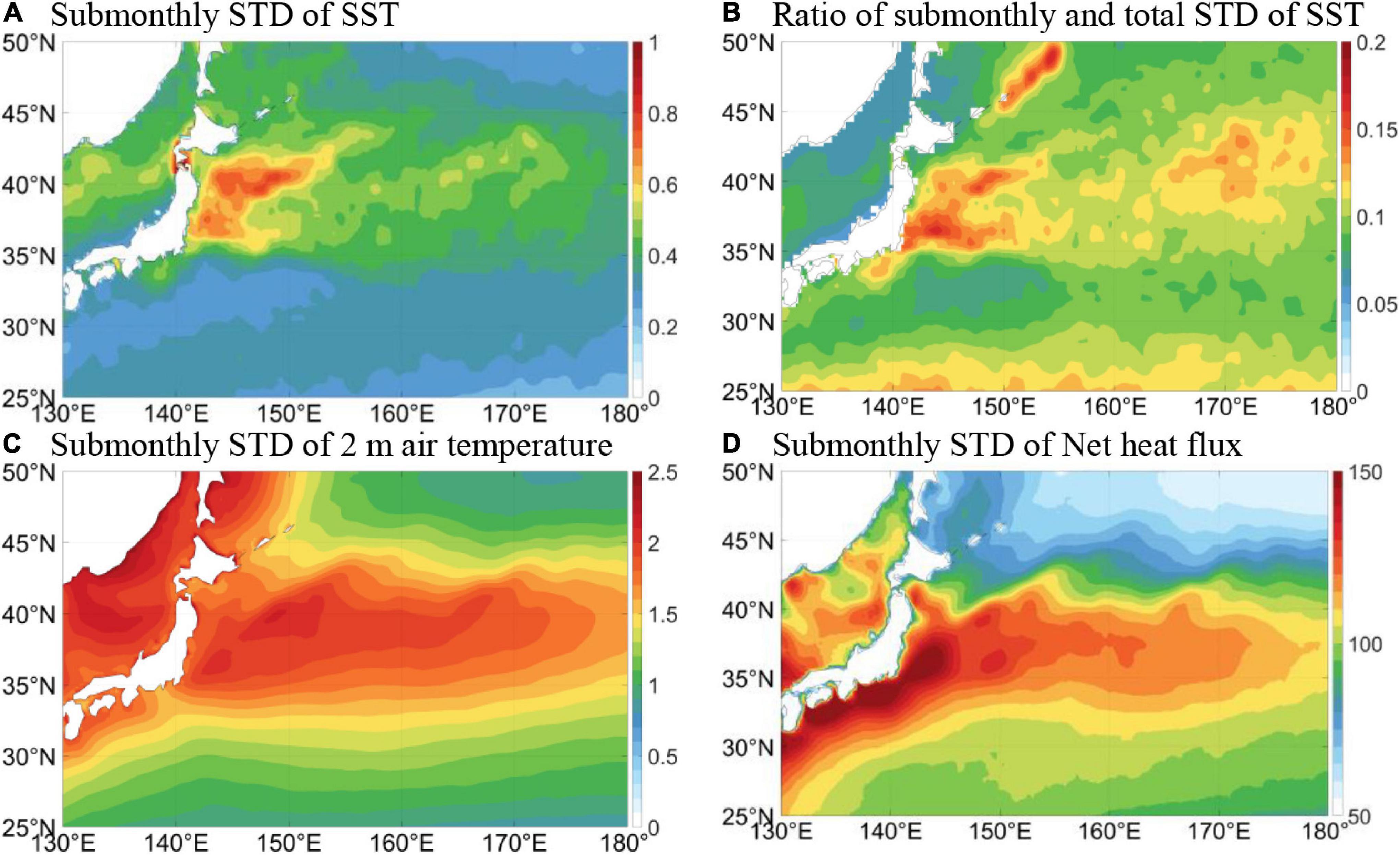
Figure 1. (A) Submonthly standard deviation of (2–30 days) SST (°C). (B) Ratio of submonthly and total standard deviation of SST. (C) Submonthly standard deviation of 2 m air temperature (°C). (D) Submonthly standard deviation of surface net upward heat flux (W/m2). All figures are based on ERA5 data in 1979–2021.
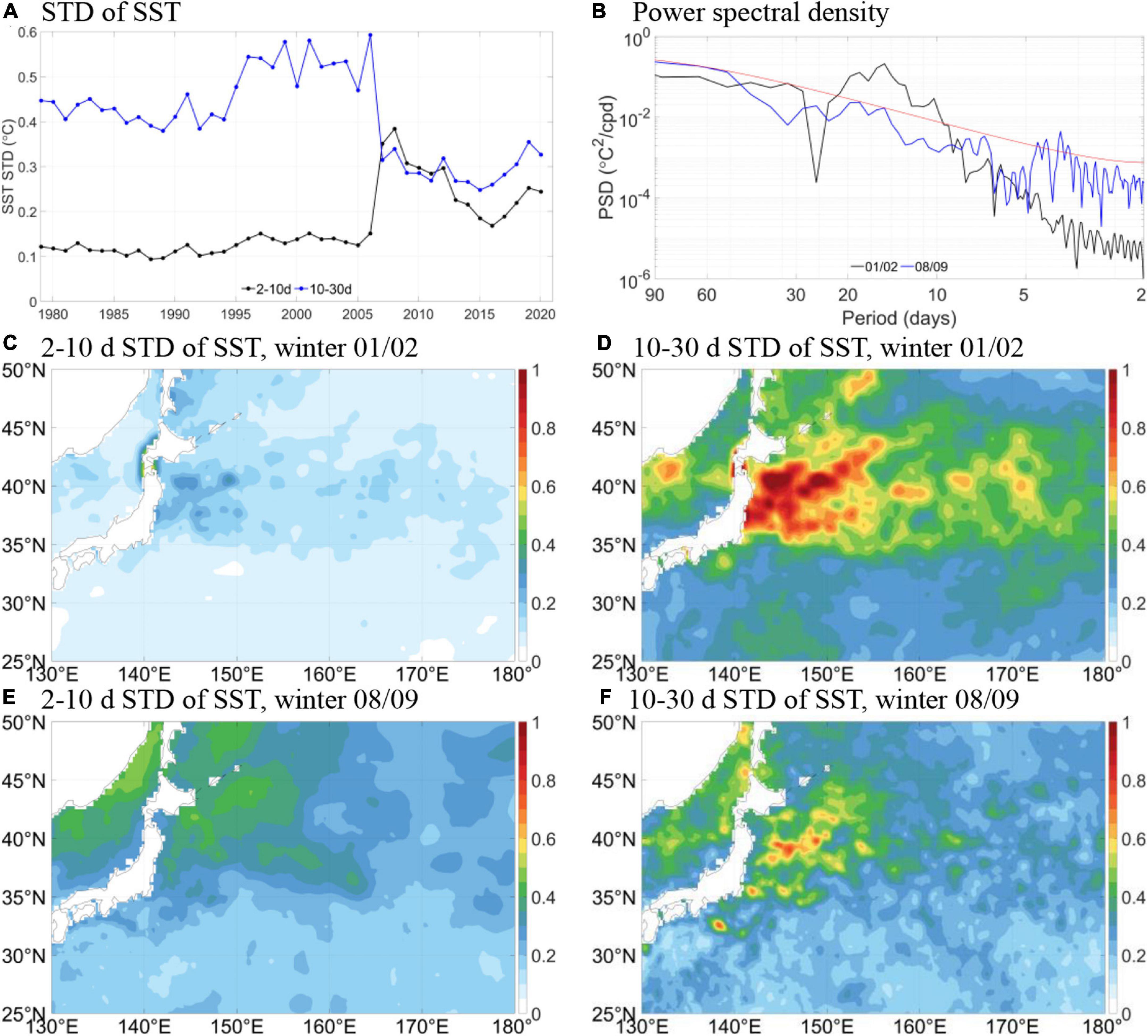
Figure 2. (A) Multi-year series of standard deviation (°C) of 2–10 days and 10–30 days SST variability in winter (DJF) averaged over the KOE region (142–155°E, 35–45°N). (B) Power spectral density (°C2/cpd) of SST at 145°E, 38°N for winter 2001/02 and 2008/09. (C) Spatial distribution of standard deviation (°C) of 2–10 days SST variability in winter 2001/02. (D) Same as (C) but for 10–30 days SST variability. (E,F) Same as (C,D) but for winter 2008/09.
The reason for the abrupt changes in SST variability is because ERA5 undergoes an update of SST boundary forcing in September 2007 from the 5-daily HadISST dataset to the daily OSTIA dataset (Hersbach et al., 2020). The temporal resolution before the update is too crude to resolve 2–10 days variability, but it becomes resolvable after the update, hence the standard deviation rises. The drop of 10–30 days standard deviation indicates that the variability on this scale before the update is too strong, probably subject to the aliasing artifact of the unresolvable higher frequencies. In the following we mainly focus on winter 2008/09 when investigating the characteristics of air-sea interaction on the two scales, and use winter 2001/02 as an opportunity to assess the potential role of different levels of SST variability on air-sea interaction. It is confirmed that selecting other representative years before and after the SST resolution shift does not change the main conclusions qualitatively. Moreover, the spatial resolution is changed from 0.25 to 0.05° along with the temporal resolution shift, but the 0.05° resolution oversamples the model grid resolution of ∼0.28°. The change of spatial resolution is, therefore, minimal.
Theoretical Considerations
Local, near-surface air-sea heat exchange can be described using the following theoretical model (Bishop et al., 2017):
where Ta and To are the air temperature and the SST, respectively. εa and εo are atmospheric and oceanic stochastic forcing terms conforming to the normal distribution. α, γa and ωa are characteristic frequencies for thermal exchange, damping, and stochastic forcing of the atmosphere. Likewise, β, γo and ωo are for the ocean. These 6 frequency parameters are all positive by definition, and their reciprocals are termed the corresponding timescales. Air-sea heat flux is represented by β(To−Ta). Incoming shortwave radiation and net thermal radiation are affected by cloud cover, not directly related to air-sea temperature difference, and are therefore not counted in the heat flux term. Latent heat flux changes SST but not surface air temperature and should therefore be included in (2) but not in (1), whereas sensible heat flux appears in both equations. This theoretical model is an extension to the classic stochastic climate model established by Hasselmann (1976) and Frankignoul and Hasselmann (1977) in which the SST variability is completely driven by atmospheric forcing (ωo = 0).
Bishop et al. (2017) solved the above model (1 and 2) numerically and argued that in case of pure atmospheric forcing, simultaneous correlation between SST and heat flux is close to zero, but simultaneous correlation between SST tendency (dT0/dt) and heat flux is negative and large. On the other hand, in case of pure oceanic forcing (ωa = 0), SST-heat flux correlation is a high positive value, but SST tendency-heat flux correlation is very small. See their Figures 1A,B for details. However, these arguments were obtained based on monthly-mean time series and a set of predefined values for the parameters α, β, γa, γo, ωa and ωo. For submonthly scales, it is unknown how the model would behave. We therefore solve the model following the method of Bishop et al. (2017), but with hourly interval and parameters more suitable for the submonthly scales. The resultant lead-lag correlation between SST/SST tendency and heat flux in pure oceanic and atmospheric forcing cases are shown in Figures 3A,B. The values of the parameters can be found in the figure caption. It is inferable that the ocean-forcing case is still characterized with strong positive SST-heat flux correlation at zero lag, reflecting the small thermal inertia of the atmosphere. In the atmosphere-forcing case, however, there exists a peak of medium-strength negative correlation between SST and heat flux when the latter leads by about a day. The SST tendency-heat flux correlation is strong and negative when heat flux is in lead of an hour which is hardly visible from the figure. This indicates that the heat obtained from the atmosphere quickly forces the SST tendency, but it takes the SST about a day to respond to this forcing. Simultaneous SST-heat flux correlation is weaker than, but of the same sign as, the peak correlation in this case.
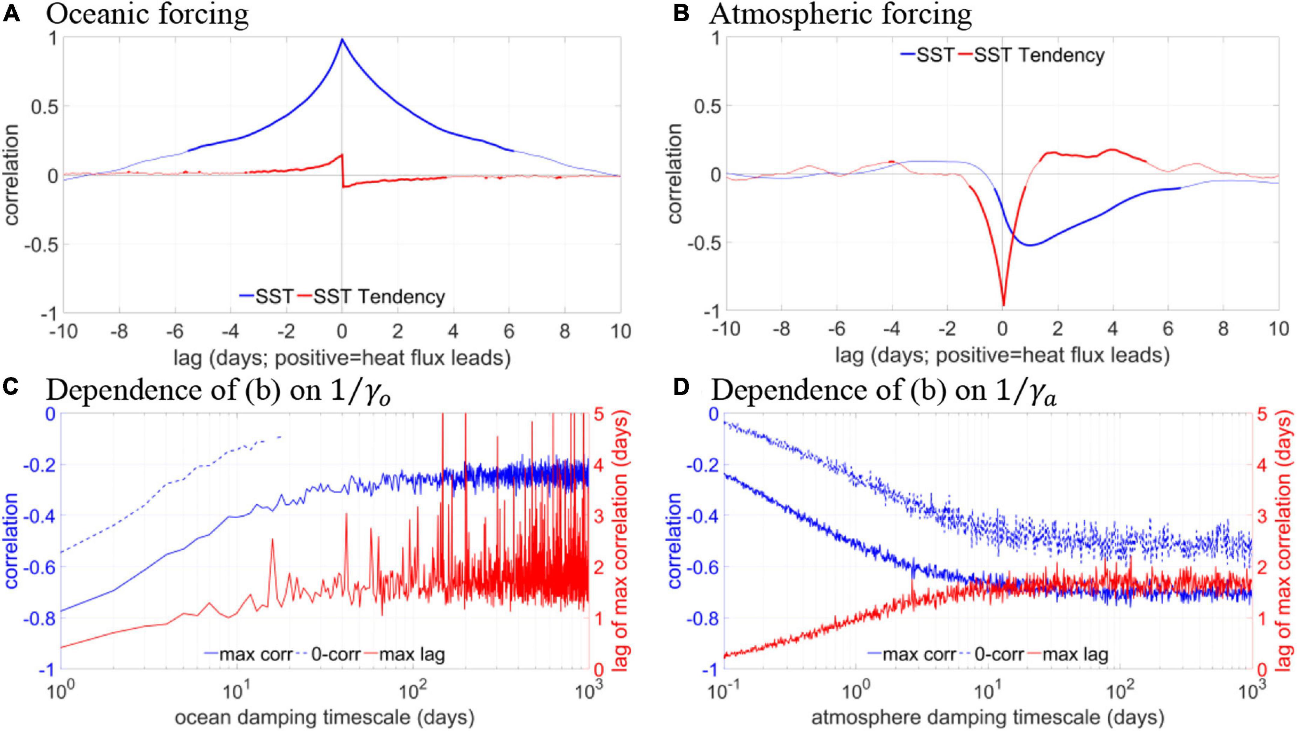
Figure 3. (A) Cross-correlation of heat flux with SST and SST tendency in the pure oceanic forcing case of the theoretical model. Here α = 1/2 d–1, β = 1/5 d–1, γa = 1 d–1, γo = 1/5 d–1, ωa = 0, ωo = 1/10 d–1. Thick parts of the curves indicate statistical significance at the 95% level. (B) Same as (A) but for the pure atmospheric forcing case. Here ωa = 1 d–1, ωo = 0, and other parameters are the same as in (A). (C) Dependence of (B) on ocean damping timescale 1/γo in terms of simultaneous correlation, maximum correlation, and time lag of maximum correlation. Only statistically significant correlation is shown. (D) Same as (C) but for dependence on atmosphere damping timescale 1/γa.
It is further confirmed that the result of Figure 3A is robust regardless of the values of the parameters, but Figure 3B, the pure atmospheric-forcing case, depends on γa and γo. The sensitivities of peak and simultaneous SST-heat flux correlations in the atmospheric-forcing case are then tested against wide ranges of γa and γo, and are shown in Figures 3C,D (note that in the figures 1/γa and 1/γo are shown). As 1/γo increases, peak SST-heat flux correlation becomes weaker, but remains statistically significant, and levels out for 1/γo ≥ 100 d. The SST response time, i.e., the time lag of the peak, increases slightly, but is mostly less than 2 days. The simultaneous correlation is always smaller than the peak value but of the same sign, weakening with increasing 1/γo and losing statistical significance for 1/γo ≥ 20 d. With increasing 1/γa, peak and simultaneous correlations both strengthen and remain significant, and the SST response time is almost always smaller than 2 days. Because the simultaneous correlation of SST-heat flux is always of the same sign as the peak value, and because its sign reverses in the pure atmospheric-forcing and pure oceanic-forcing cases, theoretically it can be used as a criterion for the direction of air-sea thermal forcing. For instance, Gulev et al. (2013) analyzed the simultaneous correlation between monthly SST and turbulent heat flux in the midlatitude North Atlantic ocean interior and found that the correlation is positive and strong on interdecadal timescales but negative and of medium strength on shorter timescales. Thereby they concluded that it is the ocean driving the atmosphere on interdecadal scales and the other way around on shorter scales, supporting the conjecture of Bjerknes (1964). Our solution using hourly interval confirms that this criterion can be extended to such small scales as submonthly, but only if the model itself is accurate. SST tendency-heat flux correlation is also sometimes used, for instance in Wu et al. (2015) who studied 10–20 and 30–60 days air-sea interaction in tropical and subtropical western North Pacific.
Observational Assessments
The pure atmospheric and oceanic forcing cases analyzed so far are extreme scenarios. In reality ωa and ωo should both be non-zero, corresponding to a mixture of forced and intrinsic SST variability. The 6 parameters must also exhibit spatial, temporal, and scale dependence. We next examine the characteristics of air-sea interaction on submonthly timescales in the framework of the theoretical model, but with objectively obtained parameters based on observations. To do so, using ERA5 SST and 2 m air temperature filtered for the 2–10 and 10–30 days scales, we estimate the parameters β and γo for each grid point in the research domain by regressing local values of dTo/dt against Ta−To and To. The residual has normal distribution by definition, and its standard deviation is assigned to ωo. Similarly, α, γa and ωa are determined for each grid point. The parameters are then substituted to the model which is solved numerically for Ta and To. Results show that the spatial pattern of ωo on the two scales (not shown) well resemble the standard deviation of SST in Figures 2E,F, indicating potential control of intrinsic oceanic perturbation on SST variability. The other parameters exhibit large ranges including negative values, resulting in unphysical temperatures over most of the domain (not shown). It is thus inferable that the theoretical model is problematic in the real ocean on submonthly timescales, most likely due to the ignorance of potentially important processes on these scales, e.g., wind mixing, convective mixing etc.
Next, we calculate SST-heat flux correlation directly from observations in ERA5. Here the heat flux is the net heat flux including all four components, i.e., sensible, latent, thermal radiation, and shortwave radiation. The simultaneous SST-heat flux correlation on 2–10 days timescale is shown in Figure 4A, with positive correlation found over much of the domain, except for the western subtropics and in the Japan Sea. In the KOE region the correlation is weak and does not exhibit obvious time-lag dependency (Figure 4B). This could probably mean that atmospheric and oceanic forcings are on the same order. On 10–30 days timescale, correlation in the KOE region becomes stronger and negative (Figure 4C), but the maximum negative correlation is found when heat flux leads by 2 days (Figure 4D). This behavior resembles the theoretic SST-heat flux correlation in the atmospheric-forcing case (Figure 3B). However, the SST tendency-heat flux correlation in Figure 4D has a negative peak when heat flux delays, in contrast to the hour-scale lead time by the heat flux as shown in Figure 3B. This indicates that the observed SST-heat flux interaction is indeed more complex than predicted by the theoretic model. A more sophisticated tool is thus required to explicitly assess the forced and intrinsic SST variability.
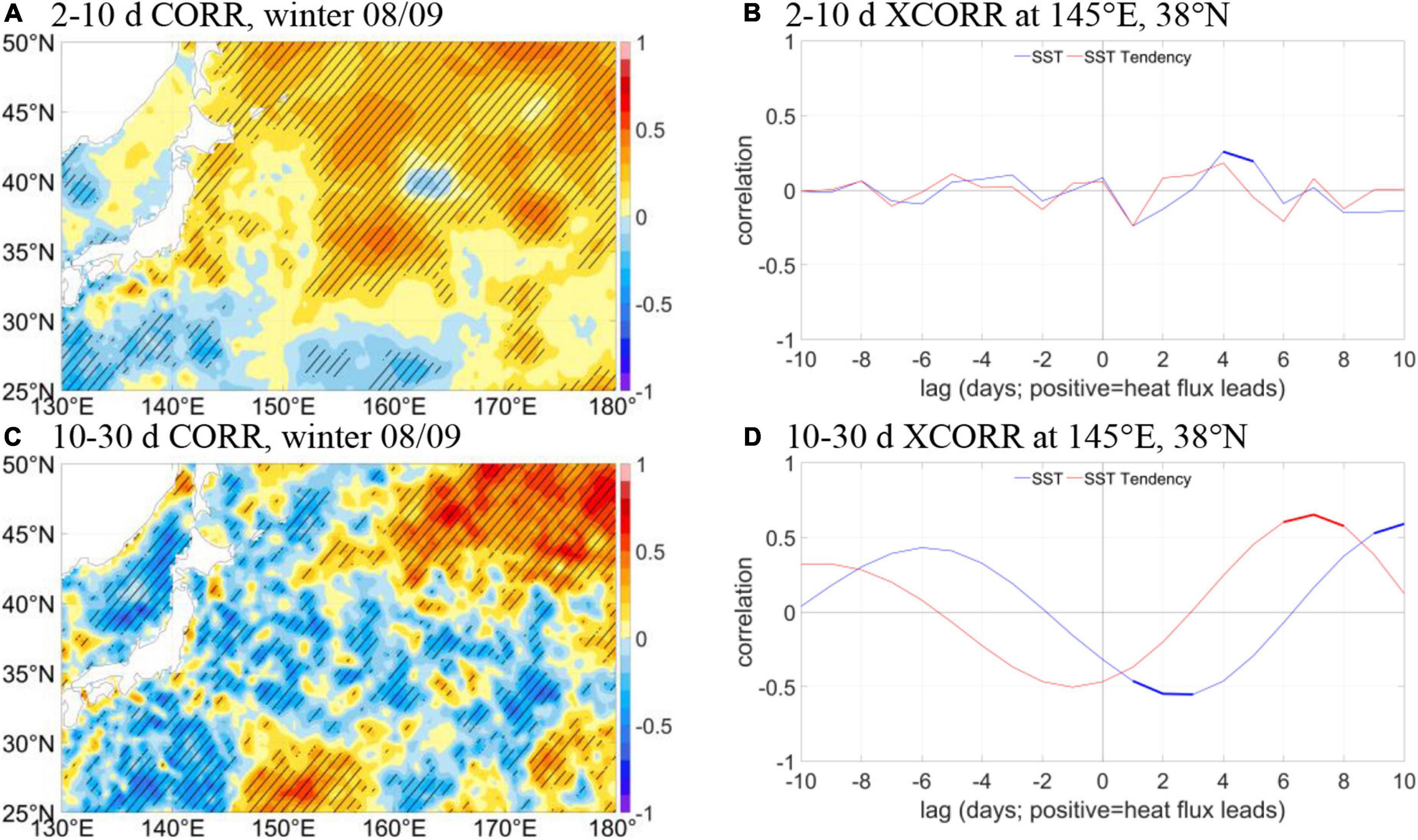
Figure 4. (A) Simultaneous correlation between SST and net heat flux on 2–10 days timescales in winter 2008/09. Hatched areas indicate statistical significance at the 95% level. (B) Cross-correlation between SST and net heat flux at 145°E, 38°N on 2–10 days timescales in winter 2008/09. Thick parts of the curves indicate statistical significance at the 95% level. (C) Same as (A) but for 10–30 days timescales. (D) Same as (B) but for 10–30 days timescales.
General Ocean Turbulence Model Results
The single-column ocean model GOTM is employed to evaluate the local SST variability forced by atmospheric perturbations. The model is forced by air-sea heat fluxes (sensible, latent, thermal radiation, and shortwave radiation), freshwater fluxes (precipitation-evaporation), and momentum fluxes (wind stress). Air-sea coupling is apparently not possible in this model, but this is deliberately chosen to obtain purely forced SST variability rather than mixed forcing and response that are hard to isolate as in the theoretical model and the observations. The model is run separately for each grid point 1.5° apart in the domain. Unlike the theoretical model which only considers the ocean surface, oceanic dynamic and thermodynamic processes in the vertical dimension, including turbulent mixing and convection, are fully captured in the model. The modeled SST variability, therefore, is forced purely, directly, and locally by the overlying atmosphere, adjusted by mechanical and buoyant mixing in the water column. On the other hand, the part of SST variability missing in the model is attributed to intrinsic local and advective oceanic processes. A set of experiments are carried out using the GOTM model, each with different combination of forcing terms. The FULL experiment, e.g., is driven by all of the 6 forcing terms, whereas the BUOY experiment uses time-varying buoyancy fluxes and constant wind stress. Experiments other than the FULL experiment are called the sensitivity experiments. See Table 1 for a summary of all the experiments.

Table 1. Comparison of physical processes in observations, the theoretical model, and the GOTM experiments.
In Figure 5A we show the ratio between the STDs of 2–10 days SST simulated by the FULL experiment and observed in ERA5. High ratios indicate higher fraction of forced SST variability than intrinsic oceanic variability, and vice versa. Since this is a forced model, it is expected that the simulated SST variability would be stronger than in a coupled model, because the SST cannot feedback to the fluxes and damp them. The STD ratio, therefore, should be interpreted as an upper bound of atmospheric-forced fraction. Statistically, the STD ratio equals the square root of the reciprocal of the F-statistics which is defined as the variance ratio between two samples. Lower (higher) STD ratio than a critical value, therefore, indicates that the modeled and observed SST has significantly different (same) variance. It is found that on the submonthly timescale, forced SST variability dominates in the western subtropics and some spots to the east and north of the KOE, in accordance with recent findings of Yu et al. (2020). In the KOE, forced variability explains a very small fraction of the total variability, suggesting the dominant role of intrinsic SST variability there. On the 10–30 days scale, as shown in Figure 5B, the percentage of forced variability in the KOE region remains very low (<10%), but outside the KOE it is even higher (> 90%). In Figures 5C,D correlations between observed and modeled SST are examined. High and significant correlations are found in the subtropical band (25–30°N) on both timescales, roughly corresponding to the regions with high standard deviation ratio, indicating that the modeled SST there is close to observation in terms of both magnitude and phase. This is the relatively quiescent region between the strong jets of the Kuroshio and its extension and the weaker Subtropical Countercurrent, both abundant in mesoscale and submesoscale processes (Yang et al., 2013; Qiu et al., 2014, 2020; Zhou et al., 2021). GOTM’s ability in simulating the forced SST variability is thus justified in regions where oceanic advection and high-frequency perturbations and are weak. We are hence able to conclude in a quantitative manner that in the strong current regions of the KOE, the dominance of oceanic internal forcing is valid on timescales as short as 2–10 days, thus extending the results of Smirnov et al. (2014) and Bishop et al. (2017). However, it should be noted that the finding based on Figure 5 contradicts Figure 4, which showed a hint of either mixed forcing or pure atmospheric forcing in the KOE according to the theoretical model. This further disqualifies the theoretical model in tackling air-sea interaction on such small timescales.
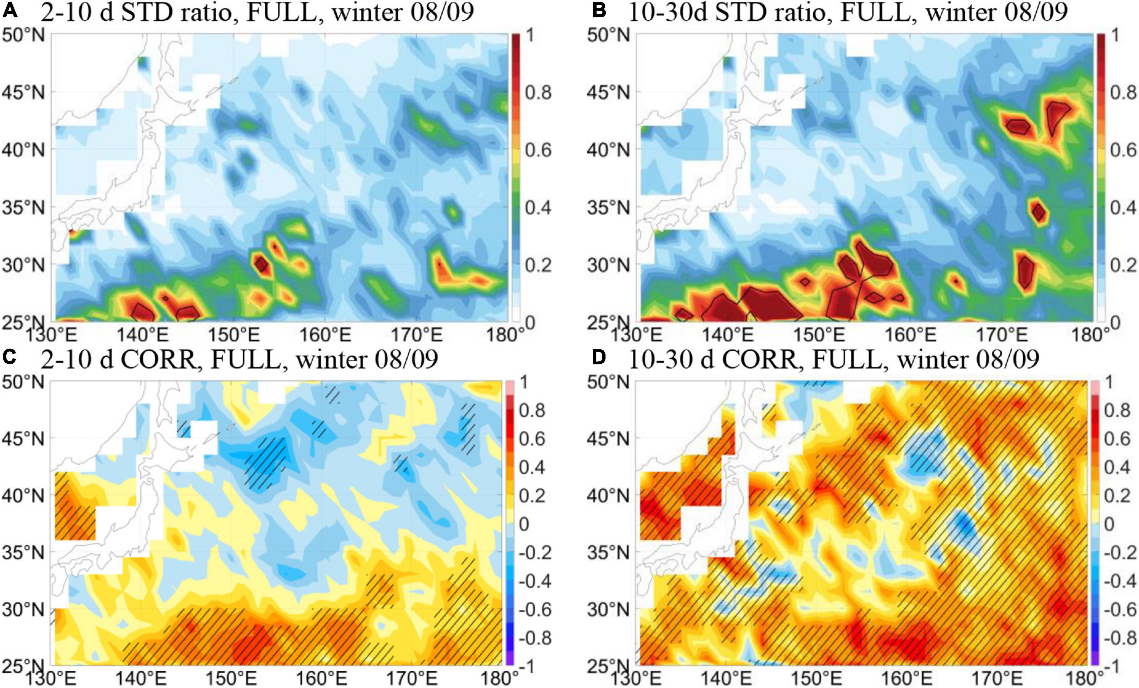
Figure 5. (Upper row) Ratio of standard deviation of SST between the GOTM-FULL experiment and observations in winter 2008/09 on (A) 2–10 days (B) 10–30 days timescales. The black contour indicates the critical ratio at the 95% significance level. (lower row) Correlation between SST of the GOTM-FULL experiment and observations in winter 2008/09 on (C) 2–10 days (D) 10–30 days timescales. Hatched areas indicate statistical significance at the 95% level.
To have a better idea on which processes are the most important, the results of the sensitivity experiments are useful. First, the SHF experiment driven solely by sensible heat flux variations exhibits different patterns of forced SST variability than in FULL (Figures 6A,B), but the percentage is still low in the KOE, except for in a small area very close to the Japanese coast. The inclusion of the latent heat flux in the THF experiment results in a STD ratio pattern resembling the FULL experiment (Figures 6C,D), indicating the importance of latent heat flux. Adding thermal radiation to THF, the NSF experiment keeps the same pattern of explained standard deviation but with reduced power (Figures 6E,F), presumably due to the damping effect of thermal radiation on SST. The NSF experiment includes the same air-sea fluxes as the theoretical model, only with the addition of vertical processes in the mixed layer. The difference between the two, therefore, reveals that only considering the sea surface is not sufficient in air-sea heat exchange on submonthly scales, and that subsurface mechanical and buoyant mixing plays a crucial role, especially in areas with deep mixed layer. Note that here the mechanical mixing is independent of wind stress. The NHF (Figures 6G,H) and BUOY (Figures 6I,J) experiments look very similar to NSF, indicating the negligible contribution from solar radiation (cloud cover) and net precipitation. Comparing the BUOY and FULL experiments, it can be found that the presence of wind stress forcing enhances the forced SST variability slightly in the KOE region and significantly in regions outside the KOE. Based on these results, three important processes have thus been identified, i.e., latent heat flux, subsurface heat exchange, and wind stress forcing (only for outside KOE). The latter two are not included in the theoretical model.
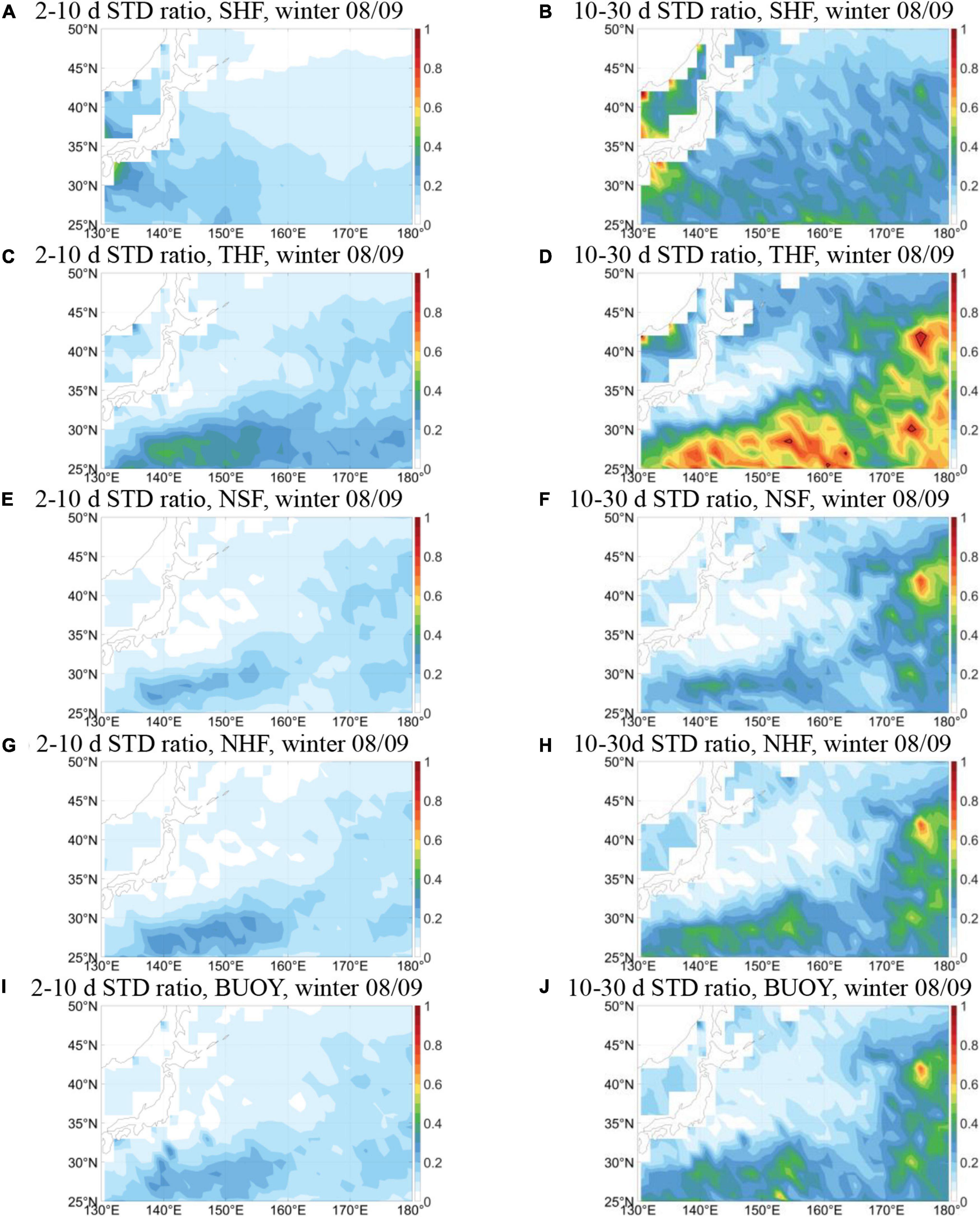
Figure 6. Ratio of standard deviation between GOTM sensitivity experiments and observations in winter 2008/09 on (A,C,E,G,I) 2–10 days and (B,D,F,H,J) 10–30 days timescales. The black contour indicates the critical ratio at the 95% significance level.
Further, the usability of correlation as an indicator for air-sea interaction is verified with the cross-correlation between the simulated SST and the net heat flux. Because the modeled SST variability is purely forced by the atmosphere, we search for the first peak (positive or negative) of the cross-correlation with increasing lead time by the heat flux. It is found that for the vast majority of the grid points in the domain, peak correlation is found at lead time of 1 day for the 2–10 days timescale, and 3 days for the 10–30 days timescale in every experiment (not shown). The spatial pattern of the peak correlation in the NSF experiment is shown in Figures 7A,B. On the 2–10 days timescale, negative correlation is found everywhere in the research domain, but on the 10–30 days scale, positive correlations occur. The possibility of positive delayed correlation even in such pure atmospheric forcing conditions is in sharp contrast to the theoretical model which requires negative delayed correlation (Figure 3B). This again suggests the deficiency of the theoretical model on these scales due to the ignorance of ocean vertical heat exchange. THF and NHF experiment results resemble the NSF (not shown), but the BUOY experiment exhibits different patterns (Figures 7C,D). The FULL experiment is similar with BUOY but with stronger positive correlations (Figures 7E,F), highlighting the role of wind stress mechanical forcing. It is therefore conclusive that the existence of vertical heat exchange and wind stress forcing in the real ocean can alter the sign of SST anomalies driven by atmospheric perturbations, thus making the SST-heat flux correlation not an appropriate tool for diagnosing the direction of air-sea interaction.
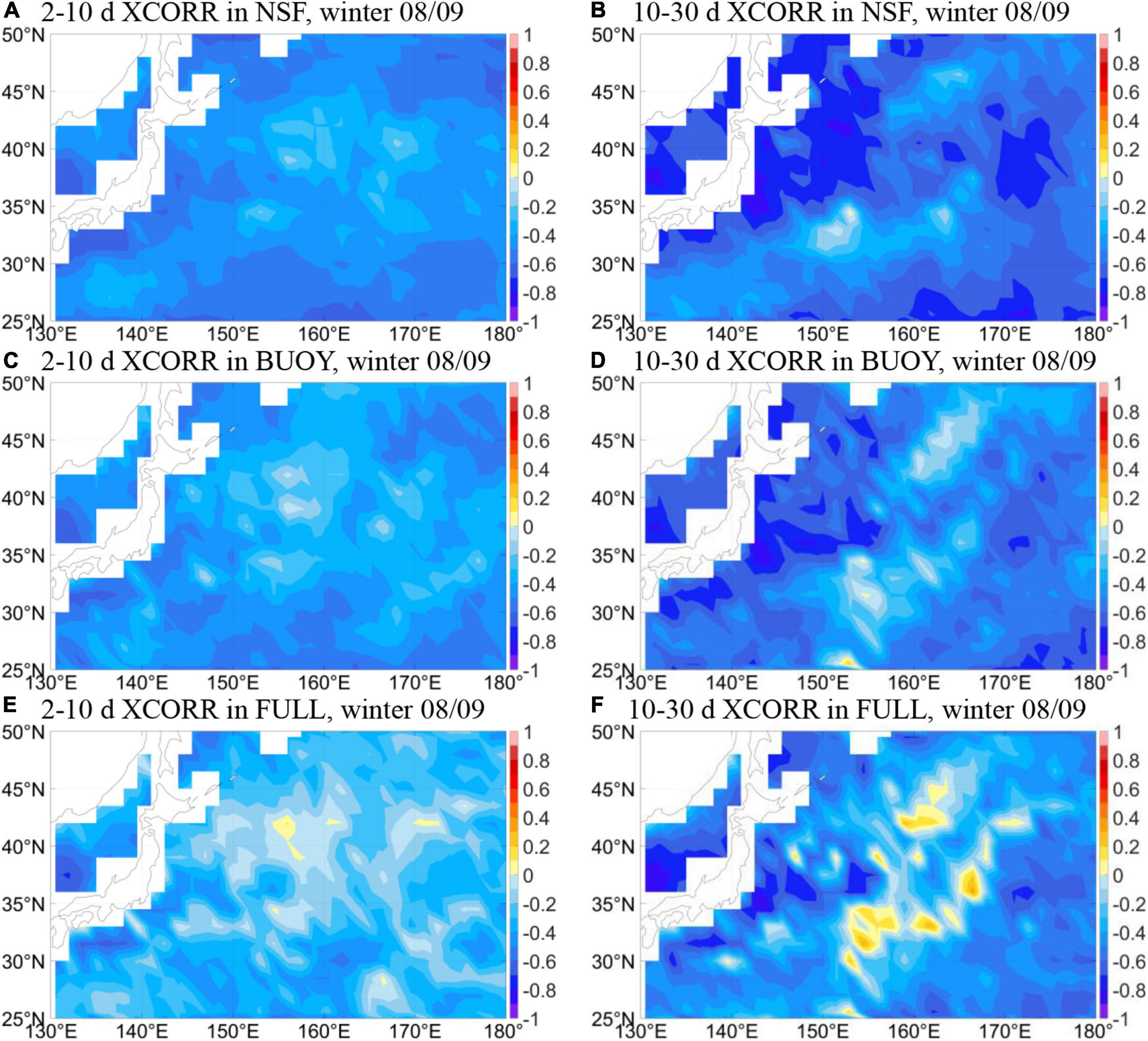
Figure 7. Delayed correlation between net heat flux and SST in selected GOTM sensitivity experiments on (A,C,E) 2–10 days and (B,D,F) 10–30 days timescales. The time lag for the 2–10 days correlation is 1 day, and for the 10–30 days correlation it is 3 days. In these figures the correlations are statistically significant at the 95% level everywhere in the domain.
Role of Different Levels of Sea Surface Temperature Variability
The previous generation of ECMWF reanalysis dataset, the ERA-Interim (Dee et al., 2011), went through enhancements of SST spatial resolution (but not temporal resolution), which has been shown to exert significant impacts on the overlying atmosphere (Zhang et al., 2020). However, potential effects of the refinement of SST temporal resolution in ERA5 (Figure 2A) are still unknown. Here, we take the view that the changed temporal resolution provides the possibility to examine the role of different levels of SST temporal variability on air-sea interaction. The above theoretical, observational, and modeling analyses are thus repeated on winter 2001/02 to compare with winter 2008/09. Figures 8A,C show the simultaneous correlation between SST and heat flux, and Figures 8B,D show the cross-correlation at 145°E, 38°N. The correlation on the 2–10 days scale is still positive but very weak, indicating mixed atmospheric and oceanic forcing. On the 10–30 days scale, unlike the medium strength negative correlation in winter 2008/09 (Figures 4C,D), the correlation is now positive and strong in the KOE. The cross-correlations of 10–30 days SST-heat flux and SST tendency-heat flux are in qualitative accordance with the oceanic-forcing case in the theoretical model (Figure 3A). The change from the atmospheric-forcing regime when 10–30 days SST variability is weak to the oceanic-forcing regime now indicates the sensitivity of the correlation tool to strength of SST disturbance. GOTM model results of the FULL experiment shown in Figures 8E,F suggest that atmospheric-driven SST variability accounts for a larger (smaller) fraction of the total variability on 2–10 days (10–30 days) timescales over the entire domain, most probably due to the weaker (stronger) total variability compared to winter 2008/09, since the forced variability is slightly weaker in winter 2001/02 on both scales (not shown). In the KOE region, however, the percentage explained by forced variability is still very small, favoring dominance of intrinsic SST variability on the two scales. Delayed correlations between SST and heat flux still exhibit positive values in the purely forced model simulations (Figures 8G,H), again disqualifying correlation as an appropriate indicator for air-sea interaction on these scales.
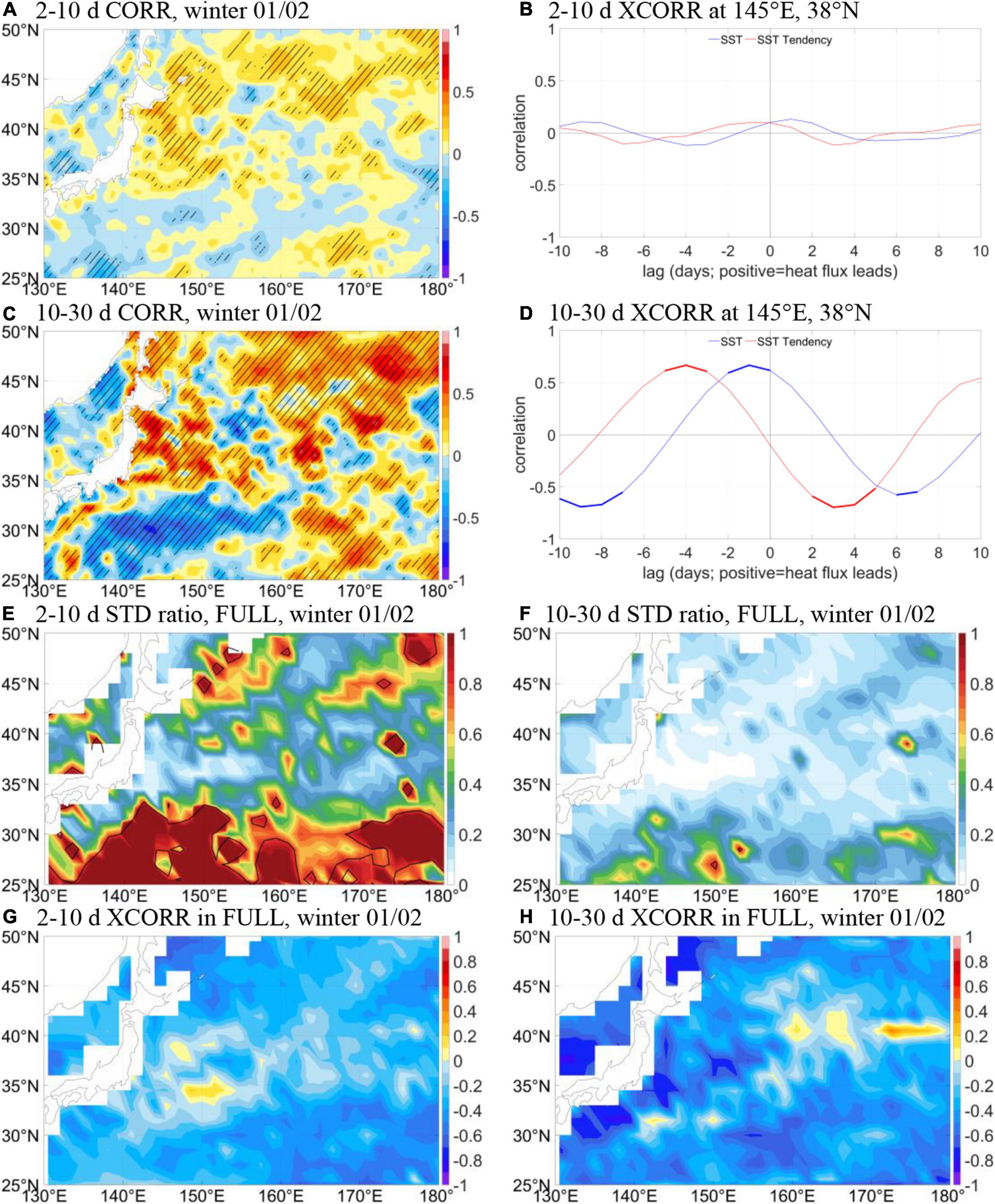
Figure 8. (A–D) Same as Figure 4 but for winter 2001/02. (E,F) Same as Figure 5 but for winter 2001/02. (G,H) Same as Figures 7E,F but for winter 2001/02.
NCEP/NCAR Results
The same analysis is performed again using the 2.5°-resolution NCEP/NCAR Reanalysis 1 dataset for winter 2008/09. SST in the NCEP/NCAR data is from the Reynolds Analysis (Smith et al., 2008) with time interval of 1 week. The 2–10 days SST variability, therefore, is poorly resolved in this dataset (Figure 9A), much like the situation of ERA5 before 2007. However, although stronger than the 2–10 days band, the 10–30 days variability (Figure 9B) is also underrepresented since a large fraction of 10–30 days SST variability is associated with mesoscale perturbations which require a much finer spatial resolution (Zhou et al., 2021). The strength of purely forced SST variability simulated by the GOTM-FULL experiment (Figures 9C,D) resembles the ERA5 results, again suggesting the importance of mixed layer processes in suppressing the direct surface response to atmospheric forcing on the submonthly scales, regardless of the spatial scale. Delayed correlations between NHF and SST (Figures 9E,F) are now negative everywhere, conforming to the pure-atmospheric driven scenario. Given the importance of wind stirring revealed above in section “General Ocean Turbulence Model Results,” this is indicative that subgrid-scale (i.e., mesoscale) anomalies of wind stress might be responsible for the reversal of NHF-SST correlation.
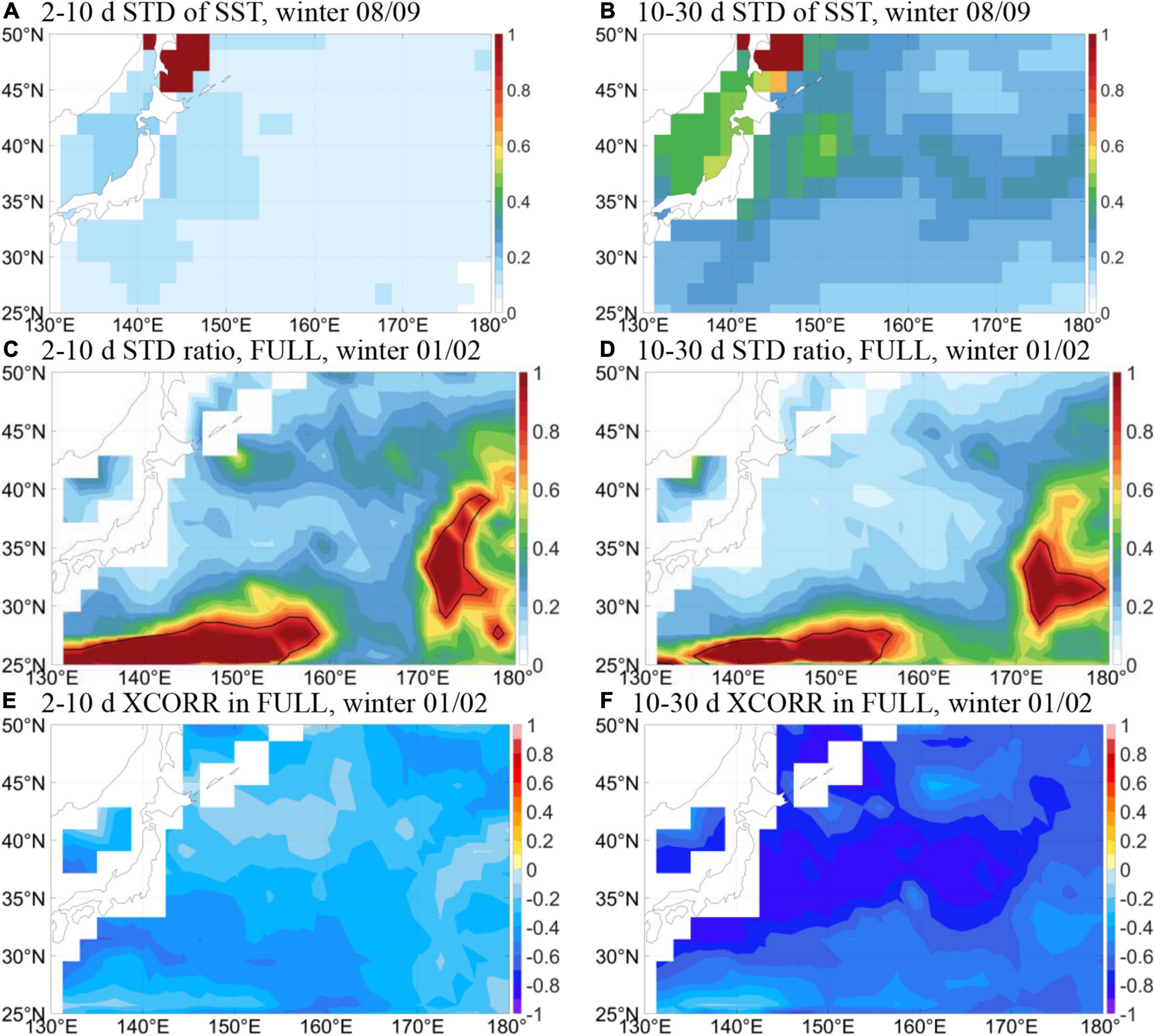
Figure 9. Results based on the 2.5-resolution NCEP/NCAR Reanalysis 1 dataset for winter 2001/02. (A,B) Correspond to Figures 2E,F, (C,D) correspond to Figures 5A,B, and (E,F) correspond to Figures 7E,F.
Summary and Conclusion
In this work we thoroughly examined the relative importance of forced and intrinsic SST variability in the KOE region on submonthly timescales (2–10 and 10–30 days) from theoretical, observational (based on ERA5), and modeling perspectives. It is shown that in the theoretical model, the pure atmospheric and oceanic forcing cases would result in different signs of simultaneous SST-heat flux correlation which is hence suitable to be used as an indicator for the direction of air-sea interaction as in previous studies on longer timescales. However, model parameters objectively estimated from observations make the model results unphysical. Direct calculation of cross-correlations of SST and heat flux based on observations gives results that are hard to interpret using the theoretical framework. The GOTM oceanic single-column model is employed as a more deterministic tool to explicitly simulate the SST variability forced by atmospheric disturbances. Results show that in the KOE region forced SST variability is responsible for a very small fraction of the total variability (< 10%) on the submonthly scales, indicating the dominance of intrinsic oceanic processes. Outside the KOE SST variability is mostly explained by forced variability. Key physical factors, namely vertical mixing in the upper ocean, wind stress forcing (mainly for outside KOE), and latent heat flux are identified with a set of sensitivity experiments. It is also concluded that SST-heat flux correlation is not a valid tool on these scales, because delayed correlations of the opposite sign than expected are found. The above results are robust against different levels of SST variability, which is tested by comparing the results in two winters before and after the upgrade of SST resolution in ERA5.
This work quantified the relative importance of forced and intrinsic SST and highlighted the dominating role of intrinsic oceanic processes in the KOE in determining the short-term SST variability on submonthly scales, and showed the different behaviors in and outside the KOE. This extends the current understanding on monthly and longer terms down to even shorter scales, and further stresses the outstanding role of strong western boundary currents in air-sea interaction. As the submonthly timescales approach the bounds of what are known in the spatial sense as “mesoscale” and “submesoscale,” this work sheds some light onto mesoscale and submesoscale air-sea interaction that is still to be studied in earnest. Our results proved the incapability of the theoretical framework on timescales as short as submonthly. More importantly, we showcased the usefulness of forced single-column ocean models in local air-sea interaction. However, it remains unclear which kinds of intrinsic oceanic processes are responsible for the submonthly SST variability. The respective roles and mechanisms of wind stirring, horizontal advection, mesoscale and submesoscale vortices, barotropic, baroclinic, and convective instabilities, etc., are to be investigated from more dynamic perspectives. The dependence of these processes on spatial and temporal resolution should also be investigated. Moreover, it is interesting whether the submonthly SST variability, which is driven intrinsically in the ocean, could force significant local responses of the overlying atmospheric boundary layer and even the free atmosphere, just as the KOE mesoscale and frontal-scale SST perturbations (Minobe et al., 2008; Small et al., 2008; Kwon et al., 2010; Ma et al., 2015; Zhou et al., 2015; Sun et al., 2018). Future studies on this issue could benefit from single-column models of the atmospheric boundary layer and/or the coupled ocean-atmosphere system.
Data Availability Statement
The original contributions presented in the study are included in the article/supplementary material, further inquiries can be directed to the corresponding author.
Author Contributions
YW performed the data analysis and model simulation and wrote the initial draft of the manuscript. GZ was behind the ideas of the work and contributed to data analysis and model simulation. GW and XC participated in the discussions and helped improve the manuscript. All authors contributed to the article and approved the submitted version.
Funding
This work was supported by the National Natural Science Foundation of China (grant no. 41906001), the Natural Science Foundation of Jiangsu Province (grant no. BK20190501), and the Fundamental Research Funds for the Central Universities (grant no. B210202137).
Conflict of Interest
The authors declare that the research was conducted in the absence of any commercial or financial relationships that could be construed as a potential conflict of interest.
Publisher’s Note
All claims expressed in this article are solely those of the authors and do not necessarily represent those of their affiliated organizations, or those of the publisher, the editors and the reviewers. Any product that may be evaluated in this article, or claim that may be made by its manufacturer, is not guaranteed or endorsed by the publisher.
Footnotes
References
Barsugli, J. J., and Battisti, D. S. (1998). The Basic Effects of Atmosphere–Ocean Thermal Coupling on Midlatitude Variability. J. Atmos. Sci. 55, 477–493. doi: 10.1175/1520-04691998055<0477:TBEOAO<2.0.CO;2
Bishop, S. P., Small, R. J., Bryan, F. O., and Tomas, R. A. (2017). Scale dependence of midlatitude air-sea interaction. J. Clim. 30, 8207–8221. doi: 10.1175/JCLI-D-17-0159.1
Bjerknes, J. (1964). ““Atlantic air-sea interaction,”,” in Advances in Geophysics, eds H. E. Landsberg and J. van Mieghem (New York: Academic Press), 1–82. doi: 10.1016/s0065-2687(08)60005-9
Brutsaert, W. (1982). Evaporation into the Atmosphere: Theory, History and Applications. Dordrecht: Springer, doi: 10.1007/978-94-017-1497-6
Burchard, H. (2002). Applied Turbulence Modelling in Marine Waters. Heidelberg: Springer, 111–115. doi: 10.1007/3-540-45419-5_5
Cayan, D. R. (1992b). Latent and sensible heat flux anomalies over the northern oceans: Driving the sea surface temperature. J. Phys. Oceanogr. 22, 859–881. doi: 10.1175/1520-0485(1992)022<0859:lashfa>2.0.co;2
Cayan, D. R. (1992c). Variability of latent and sensible heat fluxes estimated using bulk formulas. Atmosphere-Ocean 30, 1–42. doi: 10.1080/07055900.1992.9649429
Cayan, D. R. (1992a). Latent and sensible heat-flux anomalies over the northern oceans: The connection to montly atmospheric circulation. J. Clim. 5, 354–369. doi: 10.1175/1520-04421992005<0354:LASHFA<2.0.CO;2
Chang, E. K. M., Lee, S., and Swanson, K. L. (2002). Storm track dynamics. J. Clim. 15, 2163–2183. doi: 10.1175/1520-04422002015<02163:STD<2.0.CO;2
Chang, E. K. M., and Orlanski, I. (1993). On the dynamics of a storm track. J. Atmos. Sci. 50, 999–1015.
Chelton, D. B., Schlax, M. G., Freilich, M. H., and Milliff, R. F. (2004). Satellite Measurements Reveal Persistent Small-Scale Features in Ocean Winds. Science 303, 978–983. doi: 10.1126/science.1091901
Davis, R. E. (1976). Predictability of sea surface temperature and sea level pressure anomalies over the North Pacific Ocean. J. Phys. Oceanogr. 6, 249–266. doi: 10.1175/1520-04851976006<0249:POSSTA<2.0.CO;2
Davis, R. E. (1978). Predictability of Sea Level Pressure Anomalies Over the North Pacific Ocean. J. Phys. Oceanogr. 8, 233–246. doi: 10.1175/1520-04851978008<0233:POSLPA<2.0.CO;2
Dee, D. P., Uppala, S. M., Simmons, A. J., Berrisford, P., Poli, P., Kobayashi, S., et al. (2011). The ERA-Interim reanalysis: configuration and performance of the data assimilation system. Q. J. R. Meteorol. Soc. 137, 553–597. doi: 10.1002/qj.828
Deser, C., and Blackmon, M. L. (1993). Surface climate variations over the North Atlantic Ocean during winter: 1900–1989. J. Clim. 6, 1743–1753. doi: 10.1175/1520-04421993006<1743:SCVOTN<2.0.CO;2
Frankignoul, C. (1985). Sea surface temperature anomalies, planetary waves, and air-sea feedback in the middle latitudes. Rev. Geophys. 23, 357–390. doi: 10.1029/rg023i004p00357
Frankignoul, C., and Hasselmann, K. (1977). Stochastic climate models, part II application to sea-surface temperature anomalies and thermocline variability. Tellus 29, 289–305. doi: 10.3402/tellusa.v29i4.11362
Greatbatch, R. J. (1983). On the Response of the Ocean to a Moving Storm: The Nonlinear Dynamics. J. Phys. Oceanogr. 13, 357–367. doi: 10.1175/1520-04851983013<0357:OTROTO<2.0.CO;2
Gulev, S. K., Latif, M., Keenlyside, N. S., Park, W., and Koltermann, K. P. (2013). North Atlantic Ocean control on surface heat flux on multidecadal timescales. Nature 499, 464–467. doi: 10.1038/nature12268
Hasselmann, K. (1976). Stochastic climate models Part I. Theor. Tellus 28, 473–485. doi: 10.1111/j.2153-3490.1976.tb00696.x
Hersbach, H., Bell, B., Berrisford, P., Hirahara, S., Horányi, A., Muñoz-Sabater, J., et al. (2020). The ERA5 global reanalysis. Q. J. R. Meteorol. Soc. 146, 1999–2049. doi: 10.1002/qj.3803
Kistler, R., Collins, W., Saha, S., White, G., Woollen, J., Kalnay, E., et al. (2001). The NCEP–NCAR 50–Year Reanalysis: Monthly Means CD–ROM and Documentation. Bull. Am. Meteorol. Soc. 82, 247–267. doi: 10.1175/1520-04772001082<0247:TNNYRM<2.3.CO;2
Kushnir, Y. (1994). Interdecadal Variations in North Atlantic Sea Surface Temperature and Associated Atmospheric Conditions. J. Clim. 7, 141–157. doi: 10.1175/1520-04421994007<0141:IVINAS<2.0.CO;2
Kushnir, Y., Robinson, W. A., Bladé, I., Hall, N. M. J., Peng, S., and Sutton, R. T. (2002). Atmospheric GCM Response to Extratropical SST Anomalies: Synthesis and Evaluation. J. Clim. 15, 2233–2256. doi: 10.1175/1520-04422002015<2233:AGRTES<2.0.CO;2
Kwon, Y.-O., Alexander, M. A., Bond, N. A., Frankignoul, C., Nakamura, H., Qiu, B., et al. (2010). Role of the Gulf Stream and Kuroshio–Oyashio Systems in Large-Scale Atmosphere–Ocean Interaction: A Review. J. Clim. 23, 3249–3281. doi: 10.1175/2010JCLI3343.1
Latif, M., and Barnett, T. P. (1994). Causes of Decadal Climate Variability over the North Pacific and North America. Science 266, 634–637. doi: 10.1126/science.266.5185.634
Liu, W. T., Xie, X., and Niiler, P. P. (2007). Ocean–Atmosphere Interaction over Agulhas Extension Meanders. J. Clim. 20, 5784–5797. doi: 10.1175/2007JCLI1732.1
Ma, X., Chang, P., Saravanan, R., Montuoro, R., Hsieh, J.-S., Wu, D., et al. (2015). Distant Influence of Kuroshio Eddies on North Pacific Weather Patterns? Sci. Rep. 5:17785. doi: 10.1038/srep17785
Menemenlis, D., Campin, J.-M., Heimbach, P., Hill, C. N., Lee, T., Nguyen, A. T., et al. (2008). ECCO2: High resolution global ocean and sea ice data synthesis. Mercat. Ocean Q. Newsl. 31, 13–21.
Minobe, S., Kuwano-Yoshida, A., Komori, N., Xie, S.-P., and Small, R. J. (2008). Influence of the Gulf Stream on the troposphere. Nature 452, 206–209. doi: 10.1038/nature06690
Minobe, S., Miyashita, M., Kuwano-Yoshida, A., Tokinaga, H., and Xie, S.-P. (2010). Atmospheric Response to the Gulf Stream: Seasonal Variations. J. Clim. 23, 3699–3719. doi: 10.1175/2010JCLI3359.1
Nakamura, H., Lin, G., and Yamagata, T. (1997). Decadal climate variability in the North Pacific during the recent decades. Bull. Am. Meteorol. Soc. 78, 2215–2225. doi: 10.1175/1520-04771997078<2215:DCVITN<2.0.CO;2
Nonaka, M., and Xie, S.-P. (2003). Covariations of sea surface temperature and wind over the Kuroshio and its extension: Evidence for ocean-to-atmosphere feedback. J. Clim. 16, 1404–1413. doi: 10.1175/1520-0442200316<1404:COSSTA<2.0.CO;2
O’Neill, L. W., Chelton, D. B., and Esbensen, S. K. (2003). Observations of SST-induced perturbations of the wind stress field over the Southern Ocean on seasonal timescales. J. Clim. 16, 2340–2354. doi: 10.1175/2780.1
O’Neill, L. W., Chelton, D. B., Esbensen, S. K., and Wentz, F. J. (2005). High-Resolution Satellite Measurements of the Atmospheric Boundary Layer Response to SST Variations along the Agulhas Return Current. J. Clim. 18, 2706–2723. doi: 10.1175/JCLI3415.1
Price, J. F. (1981). Upper Ocean Response to a Hurricane. J. Phys. Oceanogr. 11, 153–175. doi: 10.1175/1520-04851981011<0153:UORTAH<2.0.CO;2
Price, J. F., Morzel, J., and Niiler, P. P. (2008). Warming of SST in the cool wake of a moving hurricane. J. Geophys. Res. 113:C07010. doi: 10.1029/2007JC004393
Qiu, B., Chen, S., Klein, P., Sasaki, H., and Sasai, Y. (2014). Seasonal Mesoscale and Submesoscale Eddy Variability along the North Pacific Subtropical Countercurrent. J. Phys. Oceanogr. 44, 3079–3098. doi: 10.1175/JPO-D-14-0071.1
Qiu, B., Chen, S., Klein, P., Torres, H., Wang, J., Fu, L.-L., et al. (2020). Reconstructing Upper-Ocean Vertical Velocity Field from Sea Surface Height in the Presence of Unbalanced Motion. J. Phys. Oceanogr. 50, 55–79. doi: 10.1175/JPO-D-19-0172.1
Qiu, B., Schneider, N., and Chen, S. (2007). Coupled Decadal Variability in the North Pacific: An Observationally Constrained Idealized Model. J. Clim. 20, 3602–3620. doi: 10.1175/JCLI4190.1
Ren, X., Perrie, W., Long, Z., and Gyakum, J. (2004). Atmosphere–Ocean Coupled Dynamics of Cyclones in the Midlatitudes. Mon. Weather Rev. 132, 2432–2451. doi: 10.1175/1520-04932004132<2432:ACDOCI<2.0.CO;2
Roxy, M., and Tanimoto, Y. (2012). Influence of sea surface temperature on the intraseasonal variability of the South China Sea summer monsoon. Clim. Dyn. 39, 1209–1218. doi: 10.1007/s00382-011-1118-x
Roxy, M., Tanimoto, Y., Preethi, B., Terray, P., and Krishnan, R. (2013). Intraseasonal SST-precipitation relationship and its spatial variability over the tropical summer monsoon region. Clim. Dyn. 41, 45–61. doi: 10.1007/s00382-012-1547-1
Shay, L. K., Goni, G. J., and Black, P. G. (2000). Effects of a Warm Oceanic Feature on Hurricane Opal. Mon. Weather Rev. 128, 1366–1383. doi: 10.1175/1520-04932000128<1366:EOAWOF<2.0.CO;2
Small, R. J., deSzoeke, S. P., Xie, S. P., O’Neill, L., Seo, H., Song, Q., et al. (2008). Air-sea interaction over ocean fronts and eddies. Dyn. Atmos. Ocean. 45, 274–319. doi: 10.1016/j.dynatmoce.2008.01.001
Smirnov, D., Newman, M., and Alexander, M. A. (2014). Investigating the role of ocean-atmosphere coupling in the North Pacific ocean. J. Clim. 27, 592–606. doi: 10.1175/JCLI-D-13-00123.1
Smith, T. M., Reynolds, R. W., Peterson, T. C., and Lawrimore, J. (2008). Improvements to NOAA’s Historical Merged Land-Ocean Surface Temperature Analysis (1880–2006). J. Clim. 21, 2283–2296. doi: 10.1175/2007JCLI2100.1
Sun, X., Tao, L., and Yang, X. (2018). The influence of oceanic stochastic forcing on the atmospheric response to midlatitude North Pacific SST anomalies. Geophys. Res. Lett. 45, 9297–9304. doi: 10.1029/2018GL078860
Umlauf, L., and Burchard, H. (2005). Second-order turbulence closure models for geophysical boundary layers. A review of recent work. Cont. Shelf Res. 25, 795–827. doi: 10.1016/j.csr.2004.08.004
Wallace, J. M., and Jiang, Q. (1987). “On the observed structure of the interannual variability of the atmosphere/ocean climate system,”,” in Atmospheric and oceanic variability, ed. H. Cattle (Berkshire: Royal Meteorological Society), 17–43.
Woolnough, S. J., Slingo, J. M., and Hoskins, B. J. (2000). The Relationship between Convection and Sea Surface Temperature on Intraseasonal Timescales. J. Clim. 13, 2086–2104. doi: 10.1175/1520-04422000013<2086:TRBCAS<2.0.CO;2
Wu, R. (2010). Subseasonal variability during the South China Sea summer monsoon onset. Clim. Dyn. 34, 629–642. doi: 10.1007/s00382-009-0679-4
Wu, R., Cao, X., and Chen, S. (2015). Covariations of SST and surface heat flux on 10-20 day and 30-60 day time scales over the South China Sea and western North Pacific. J. Geophys. Res. Atmos. 120, 12486–12499. doi: 10.1002/2015JD024199
Wu, R., Kirtman, B. P., and Pegion, K. (2008). Local rainfall-SST relationship on subseasonal time scales in satellite observations and CFS. Geophys. Res. Lett. 35, L22706. doi: 10.1029/2008GL035883
Xie, S.-P. (2004). Satellite Observations of Cool Ocean–Atmosphere Interaction. Bull. Am. Meteorol. Soc. 85, 195–208. doi: 10.1175/BAMS-85-2-195
Xie, S.-P., Hafner, J., Tanimoto, Y., Liu, W. T., Tokinaga, H., and Xu, H. (2002). Bathymetric effect on the winter sea surface temperature and climate of the Yellow and East China Seas. Geophys. Res. Lett. 29, 81–81. doi: 10.1029/2002GL015884
Yang, G., Wang, F., Li, Y., and Lin, P. (2013). Mesoscale eddies in the northwestern subtropical Pacific Ocean: Statistical characteristics and three-dimensional structures. J. Geophys. Res. Ocean. 118, 1906–1925. doi: 10.1002/jgrc.20164
Yelland, M., and Taylor, P. K. (1996). Wind Stress Measurements from the Open Ocean. J. Phys. Oceanogr 26, 541–558. doi: 10.1175/1520-04851996026<0541:WSMFTO<2.0.CO;2
Yu, J., Gan, B., Jing, Z., and Wu, L. (2020). Winter Extreme Mixed Layer Depth South of the Kuroshio Extension. J. Clim. 33, 10419–10436. doi: 10.1175/JCLI-D-20-0119.1
Zhang, C., Liu, H., Xie, J., Li, C., and Lin, P. (2020). Impacts of Increased SST Resolution on the North Pacific Storm Track in ERA-Interim. Adv. Atmos. Sci. 37, 1256–1266. doi: 10.1007/s00376-020-0072-0
Zhou, G. (2019). Atmospheric Response to Sea Surface Temperature Anomalies in the Mid-latitude Oceans: A Brief Review. Atmosphere-Ocean 57, 319–328. doi: 10.1080/07055900.2019.1702499
Zhou, G., Latif, M., Greatbatch, R. J., and Park, W. (2015). Atmospheric response to the North Pacific enabled by daily sea surface temperature variability. Geophys. Res. Lett. 42, 7732–7739. doi: 10.1002/2015GL065356
Zhou, G., Latif, M., Greatbatch, R. J., and Park, W. (2017). State Dependence of Atmospheric Response to Extratropical North Pacific SST Anomalies. J. Clim. 30, 509–525. doi: 10.1175/JCLI-D-15-0672.1
Keywords: midlatitude, submonthly variability, air-sea interaction, stochastic climate model, GOTM model
Citation: Wu Y, Zhou G, Wang G and Cheng X (2022) Forced vs. Intrinsic Wintertime Submonthly Variability of Sea Surface Temperature in the Midlatitude Western North Pacific. Front. Mar. Sci. 9:847144. doi: 10.3389/fmars.2022.847144
Received: 01 January 2022; Accepted: 23 February 2022;
Published: 23 March 2022.
Edited by:
Zhiyu Liu, Xiamen University, ChinaReviewed by:
Bolan Gan, Ocean University of China, ChinaJing Ma, Nanjing University of Information Science and Technology, China
Copyright © 2022 Wu, Zhou, Wang and Cheng. This is an open-access article distributed under the terms of the Creative Commons Attribution License (CC BY). The use, distribution or reproduction in other forums is permitted, provided the original author(s) and the copyright owner(s) are credited and that the original publication in this journal is cited, in accordance with accepted academic practice. No use, distribution or reproduction is permitted which does not comply with these terms.
*Correspondence: Guidi Zhou, Z3VpZGkuemhvdUBoaHUuZWR1LmNu
 Yusheng Wu
 Guidi Zhou
 Guifen Wang
 Xuhua Cheng