Effects of Internal Climate Variability on Historical Ocean Wave Height Trend Assessment

This study assesses the effects of internal climate variability on wave height trend assessment using the d4PDF-WaveHs, the first single model initial-condition large ensemble (100-member) of significant wave height (H_s) simulations for the 1951–2010 period, which was produced using sea level pressure taken from Japan’s d4PDF ensemble of historical climate simulations. Here, the focus is on assessing trends in annual mean and maximum H_s. The result is compared with other model simulations that account for other sources of uncertainty, and with modern wave reanalyses. It is shown that the trend variability arising from internal climate variability is comparable to the variability caused by other factors, such as climate model uncertainty. This study also assesses the likelihood to mis-estimate trends when using only one ensemble member and therefore one possible realization of the climate system. Using single member failed to detect the statistically significant notable positive trend shown in the ensemble in some areas of the Southern Ocean. The North Atlantic Ocean is found to have large internal climate variability, where different ensemble-members can show trends of the opposite signs for the same area. The minimum ensemble size necessary to effectively reduce the risk of mis-assessing H_s trends is estimated to be 10; but this largely depends on the specific wave statistic and the region of interest, with larger ensembles being required to assess extremes. The results also show that wave reanalyses are not suitable for analyzing H_s trends due to temporal inhomogeneities therein, in agreement with recent studies.

1 Introduction

Waves are an important element of the climate system, modulating interactions between oceans and atmosphere (Cavaleri et al., 2012). They are also a key environmental variable for coastal and offshore engineering (International Organization for Standarization, 2007; Gudmestad, 2020), navigation planning (Grifoll et al., 2018), and are a potential source of renewable energy (Reguero et al., 2019). Furthermore, waves are important drivers of coastal dynamics processes, such as coastal erosion (Stive et al., 2002; Huppert et al., 2020), and contribute to sea-level extremes at multiple time scales (Melet et al., 2018; Melet et al., 2020). This is critical as over 300 million people live on low-lying coastal areas (Griggs and Reguero, 2021).

Detailed knowledge of wave climate is essential to address the aforementioned environmental and societal impacts. However, our current understanding is affected by several sources of uncertainty, as highlighted by Morim et al. (2019), who presented the latest comprehensive large ensemble of global wave projections. They found a large uncertainty in the historical annual mean significant wave height (H_s) climatology with discrepancies exceeding 20% in some areas. The climate model and the method to simulate ocean waves were found to be dominant uncertainty factors. However, the wave method uncertainty, as defined in Morim et al. (2019), included uncertainty factors beyond the mere relationship between atmospheric forcing and wave parameters, as some of the wave methods bias-corrected the forcing drivers (using different wave reanalysis as reference) while others used atmospheric forcing as directly output by climate models. Therefore, this wave method uncertainty implicitly included factors related to different atmospheric model parameterizations and data assimilation associated to the corresponding reference datasets used for calibration.

Despite the recent coordinating efforts to better characterize waves, the role of internal climate variability, and particularly its effects on trend assessment, is still poorly known. Morim et al. (2019) only accounted for one realization per model and scenario combination. Wang et al. (2015) considered multi-run H_s simulations but these had 10 runs per model/scenario at most, and the study focused on signal uncertainty rather than trend assessment. Recently, Song et al. (2021) developed centuries of global ocean wave data, including 165-year (1850-2014) of historical data. Despite being a unique database for ocean wave climate research, it only simulates one realization given the same climatological forcing. In terms of the driving wind fields, Morim et al. (2020) found that the underlying physics of the atmospheric component of climate models is the dominant source of bias in simulated wind fields, and that inter-model uncertainty is typically 2-4 times larger than the uncertainty associated with internal variability. However, they used a relatively small sample (3-10 model realizations).

Historical simulations are one possible realization of the climate system within its boundaries of internal variability. Studies based on single model realizations might underestimate extreme events or confound trends with internal (climate) variability. For example, internal variability can mask or enhance human-induced sea-ice loss on timescales ranging from years to decades (Swart et al., 2015). Also, differences between models or a model and observations can easily be misinterpreted as significant differences, while they could be simply caused by an insufficient sample size (Milinski et al., 2020). For instance, at least thirty ensemble members are required for a robust estimate of El Niño-Southern Oscillation (ENSO) variability, which plays a primarily positive role in intensifying anomalous wave climate (Yang and Oh, 2020). In terms of annual hurricane frequency, Mei et al. (2019) concluded that twenty ensemble was sufficient to detect year-to-year variations. The number of ensemble members required for robust estimates depends on targets or on temporal and spatial averaging scale (Ishii and Mori, 2020).

Despite the increasing amount and type of observations (mostly thanks to satellite records since 1979) and the continuous development of climate models, there are still many challenges in the characterization of the historical wave climate and the trends therein. State-of-the-art wave reanalysis and hindcasts present notable discrepancies and even exhibit opposite trends at global and regional scales (Sharmar et al., 2020). For example, modern reanalyses simulate contrasting positive and negative statistically significant trends in the annual mean H_s of the South Atlantic (of up to 0.05 m/decade in absolute value). The inconsistencies of reanalysis data sets are due to the changing quantity and quality of the satellite data incorporated into the products (Stopa et al., 2019). Discrepancies were also obtained by Dodet et al. (2020) when comparing the trends derived from satellite records after considering two different post-processing data approaches. To date, wave climate studies have focused on uncertainties related to model resolution and parameterizaton, downscaling methods, observations errors and data assimilation but there is little knowledge about the role of internal wave climate variability.

A Single Model Initial-condition Large Ensemble (SMILE) is a set of simulations conducted using a single model with identical external forcing and a large ensemble of different initial conditions (Maher et al., 2021). SMILEs are valuable data to investigate the climate system as they can help separate internal climate variability of the forced system from the forced response to changes in external forcing, and to sample extreme events with large return periods (Maher et al., 2021). For example, they are beneficial for robust attribution of climate changes to anthropogenic forcing (Kirchmeier-Young et al., 2021), and to investigate the uncertainty associated to compound events (Santos et al., 2021).

Here we present and analyze the first SMILE-based ensemble of global ocean significant wave height (H_s) simulations, which was produced using the 100-member ensemble of mean sea level pressure (SLP) taken from Japan’s d4PDF ensemble of historical climate simulations (Mizuta et al., 2017). After a slight modification in two of the 11 modelling regions (the tropical Pacific regions were split into two, see Section 2.1), the statistical model developed by Wang et al. (2012, 2014) was used to obtain the wave heights driven by d4PDF SLP fields. This study investigates for the first time the role of internal climate variability in trend assessment of ocean wave heights at global scale. This helps to gain insight in the understanding of historical wave conditions and changes therein, bringing additional perspective in the context of the aforementioned discrepancies in modern reanalysis/hindcast products.

2 Materials and Methods

2.1 d4PDF-WaveHs

The d4PDF-WaveHs ensemble analyzed in this study is a SMILE-based ensemble of global historical H_s. This ensemble consists of 100 members of 6-hourly H_s for the period 1951–2010 on a 1°× 1° lat.-long. grid over the global oceans. It was produced using an advanced statistical model with SLP-based predictors derived from the SLP historical simulations taken from the d4PDF large ensemble, which includes historical climate and future projections (Mizuta et al., 2017). The 60 km resolution atmospheric global circulation model (AGCM) MRI-AGCM developed by the Japan Meteorological Research Institute was used to generate d4PDF (Mizuta et al., 2012). The 100 historical simulations constitute a SMILE-type ensemble as they were generated by perturbations of the historical sea surface temperature (SST), sea ice concentration (SIC) and sea ice thickness (SIT) in relation to the observed errors (while using the same forcing, and global mean concentration of greenhouse gases (GHG) based on observations). More than 70 papers related to d4PDF have been published to date, including impact assessment and social implementation studies (Ishii and Mori, 2020). d4PDF satisfactorily simulates the past climate in terms of climatology, natural variations, and extreme events such as tropical cyclones (Ishii and Mori, 2020).

To be able to generate 6,000 years (100 × 60 years) of H_s data with a reasonable computational cost, the statistical model developed by Wang et al. (2012, 2014) was used to produce the d4PDF-WaveHs. This method consists of a multivariate regression model with lagged-dependent variable to represent the relationship between H_s and SLP-derived predictors (anomalies of SLP and squared SLP gradients), including leading principal components of large areas to account for swell waves. In particular, the 6-hourly H_s at a target wave grid point (of the 1°× 1° lat.-long grid) is simulated with a mutlivariate regression model of the form:

$\begin{array}{ll}{H}_t=a+\sum _{k=1}^K{b}_k{X}_{k,t}+\sum _{p=1}^P{c}_p{H}_{t-p}+u_t& (1)\end{array}$

where H_t is the Box-Cox transformed H_s (Box and Cox, 1964), X_k,t are the K selected SLP-based predictors, P is the order of lags of the dependent variable (the predictand) and the residuals u_t are modelled as an M-order autoregressive process. The Box-Cox transformation is applied to bring the residuals close to a normal distribution, as assumed in the regression analysis. The SLP-based predictors consist of a pool of 62 potential predictors: the anomalies (relative to the 1981–2000 mean) of, respectively, SLP and the squared SLP gradient (which represents the geostrophic wind energy) and their respective 30 leading principal components over a selected area to represent the large scale patterns of atmospheric circulation affecting the wave climate of a target grid point. A forward model-selection procedure with F test with equivalent sample size (vonStorch and Zwiers, 1999) was used to determine the K selected SLP-derived predictors [see Eq. (1)] for a target wave grid point. The P and M values were also determined using the F test with the equivalent sample size. To account for seasonality of atmospheric circulation regimes, H_s is modelled in each of the four seasons separately. More details of this statistical modelling approach can be found in Wang et al. (2012, 2014). Note that the two tropical Pacific regions, TNP and TSP (the two largest regions) in Wang et al. (2012, 2014) were each split into two regions (ETNP, WTNP, ETSP, WTSP); so that the model was calibrated for 13 regions over the globe in this study (rather than 11 regions; see Figure 1). The smaller regions slightly improved the model skill for those regions.

FIGURE 1

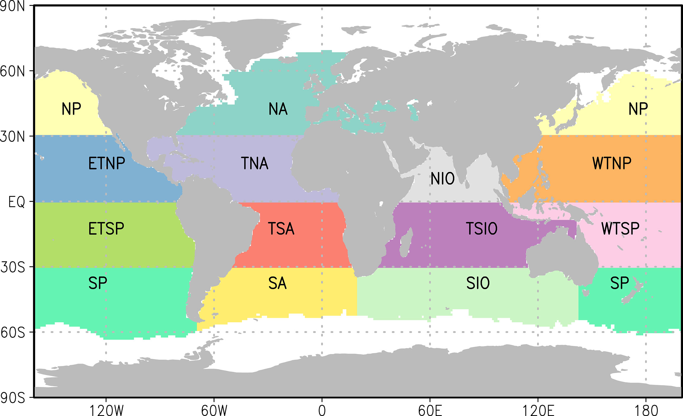
Figure 1 Areas used to calibrate the wave model and compute the regional averaged trends and time series.

As in Wang et al. (2014), Eq. (1) was calibrated and evaluated using the European Center for Medium-Range Weather Forecasts (ECMWF) Reanalysis Interim (ERAint) (Dee et al., 2011). Before calculating the X_k,t predictors to produce the H_s simulations, the d4PDF-WaveHs SLP fields were adjusted to have the same climatological mean and standard deviation as the ERAint SLP data. As explained in Wang et al. (2014), this is needed in order to apply the Box-Cox transformations which were optimized for the ERAint data. Additionally, we excluded (set to missing) any simulated H_s values that exceed twice the largest H_s from ERAint for a given season. This cap is needed as, very rarely, the Box-Cox transformation of the SLP gradients leads to an overgrowth of the sharp SLP gradients of rapidly forming low pressure centers which, in turn, leads to unrealistic H_s values. This is arguably caused by the higher spatial resolution of the d4PDF SLP fields, as compared to ERAint, which might be able to simulate stronger SLP gradients than those generated by ERAint. However, note that this overgrowth is extremely rare and occurs with a frequency of less 0.05‰ in all simulated H_s data.

This statistical wave modelling approach to simulate H_s has been used and validated in many studies to derive regional and global historical/future H_s datasets and to assess trends, projected changes and variability (Wang et al., 2012; Wang et al., 2014; Wang et al., 2015). For example, it was used to derive one of the contributing datasets of the latest coherent, community-driven, multi-method ensemble of global wave climate projections (Morim et al., 2019). In this study, we further assessed the reliability of the statistical modelling method by comparing the resulting trends of the annual mean and maximum H_s as obtained from one member of the d4PDF-WaveHs with those derived from the traditional dynamical modelling approach for the same d4PDF member. The single-member dynamical wave simulations were conducted using WAVEWATCH III (WW3) driven by the surface wind fields of the d4PDF member in question. We used the same WW3 version (5) and model configuration as in Shimura and Nobuhito (2019) which has a spatial resolution of ~ 0.5°. For both datasets, the annual mean H_s trend is remarkably positive in the Southern Ocean but the statistical approach simulates a less intensive tendency to increase over a smaller area (Figure S1). This can be arguably explained by the lower spatial resolution of the simulations obtained with the statistical modelling approach (1°) in comparison to the WW3 simulations (~ 0.5°). Indeed, there is a better agreement in terms of the trends relative to the 1951–2010 climatological mean, as they are less affected by spatial resolution (see Figure S2). For the annual maximum H_s, both approaches simulate a nosier spatial pattern of trends than for the annual mean H_s, as expected for this extreme statistic. For both datasets, positive increases in the annual maximum H_s are seen in the Southern Ocean and in the Northern Pacific, Northern Atlantic and Indian Oceans. Overall, the results show that the statistical and dynamical methods are in reasonably good agreement with each other, showing similar spatial patterns of trends for both the annual mean H_s and maximum H_s.

2.2 Trend Analysis

This study focuses on the assessment of the annual mean and maximum H_s trends for the period 1951–2010 and the uncertainty derived from the internal climate variability. First, individual trends were computed for each ensemble member of d4PDF-WaveHs using the (non-parametric) Mann-Kendall method with lag-1 autocorrelation being accounted for (Wang and Swail, 2001). Second, the individual-member trends were averaged over the 100 ensemble members to obtain the ensemble averaged trend. Then, the regional average trends are calculated as the average over all gridpoints in each of the modelling areas shown in Figure 1.

At a given grid point, the ensemble averaged trend is considered statistically significant if >50% of the individual-member trends are significant at the 5% level, and >90% of these significant individual-member trends have the same trend sign. This method was used by Morim et al. (2019) as it was identified as a suitable method to identify regions of robustness (IPCC, 2013). As discussed later in the manuscript, this method is more restrictive than performing a t-test on the individual trend estimates, as the latter does not account for the inter-annual variability.

In addition, we investigate the impact of internal climate variability on the results of trend assessment, showing what we can gain from using a SMILE-based ensemble. In particular, we estimated the following three likelihoods:

1. the likelihood for an ensemble member to have the same trend conclusion as the ensemble averaged trend. Here trend conclusion is one of the following three outcomes: (a) statistically significant positive trend, (b) statistically significant negative trend, (c) statistically insignificant trend (regardless of the sign).

2. the likelihood for an ensemble member to have the same trend sign as the ensemble averaged trend, regardless of the significance level.

3. the likelihood for an ensemble member to give a trend conclusion that is opposite to that of the ensemble, showing a statistically significant trend of the opposite sign to the ensemble average trend (here both trend estimates are statistically significant).

We repeated the above analysis by considering x-size sub-ensembles (randomly sampled 100 times from d4PDF-WaveHs), where x goes from 2 to 50. This allows us to investigate the gain from using gradually larger ensembles, and to find the optimal ensemble size for estimating trend in the two H_s statistics analyzed.

2.3 Wave Datasets Used for Comparison

For comparison purposes, the trend assessment described in Section 2.2 is also performed for state-of-the-art wave reanalysis both at global and regional scales, as well as on a grid point basis. The goal is put the role of the internal climate variability for trend assessment (based on d4PDF-WaveHs) into perspective of the estimates and discrepancies among modern reanalysis datasets. In particular, we used the second version of the National Centers for Environmental Prediction (NCEP) Climate Forecast System Reanalysis (CFSR) (Saha et al., 2014), ERAint (Dee et al., 2011) and the more recent ECMWF 5^th generation reanalysis (ERA5) (Herbach et al., 2020). Although ERA5 is available since 1950, we consider a common period of analysis from 1979 to 2009 for these three reanalysis datasets.

Additionally, we compared our trend estimates and uncertainty results with those obtained from historical wave simulations without data assimilation. First, we use the historical CMIP5-driven dataset developed by Wang et al. (2014), hereafter called CMIP5-HsWang, which used the same statistical modelling approach as this study. CMIP5-HsWang provides 6-hourly H_s produced using SLP simulations by 20 climate models (only one realization per model) for the period 1950–2005. With this comparison we investigate how internal climate variability compares to model variability in terms of trend estimates. Despite the forcing SLP data being adjusted to have the same climatological mean and variance as the ERAint SLP data, model variability was identified by Wang et al. (2014) as one major factor of uncertainty that is significantly different from zero globally.

Finally, we also performed the same trend analysis with the 1979–2004 COWCLIP historical ensemble (Morim et al., 2019), referred to as CMIP5-COWCLIP hereafter, which mainly accounts for climate model variability and wave method variability. Morim et al. (2019) identified both of these factors as key sources of uncertainty, with different contributions to total uncertainty depending on the region. Here we consider the 48 members that provide both annual mean and annual maximum H_s.

3 Results

The ensemble average of trends in the annual mean H_s for the period 1951–2010, as simulated by d4PDF-WaveHs is positive and statistically significant (at 5% level) in the Southern Ocean with rates exceeding 0.5 cm/yr (Figure 2A), which represent an increase of up to 0.25%/yr relative to the 1951–2010 climatological mean (see Figure S3A). This rate of increase outstands from the rest of the oceans, which have positive/negative rates of up to 0.3 cm/yr in absolute value. This is reasonable given the more energetic wave climate of this unique continuous body of water encircling the Earth affected by continuous low pressure systems. Trends are also positive and statistically significant in areas of the tropical west Pacific, the southern East Pacific, the Southern Atlantic and the Indian Ocean. The only area with statistically significant negative trend is located south of Africa. A similar pattern is observed for the ensemble average of trends in the annual maximum H_s (Figures 2B and S3B) but in this case the trends are statistically insignificant, and the latitudinal gradient between the Southern Ocean trends and the rest of the oceans is lower. Simulations of the annual maximum H_s trend show a nosier spatial pattern than for the annual mean H_s counterpart (see Figures S4−S7) due to the inherent additional uncertainty associated to extremes. This noise is implicitly reflected in the ensemble averaged trend with a lower statistical significance associated to the annual maximum H_s trends, as compared to those of the annual mean H_s (Figure 2A vs. Figure 2B).

FIGURE 2

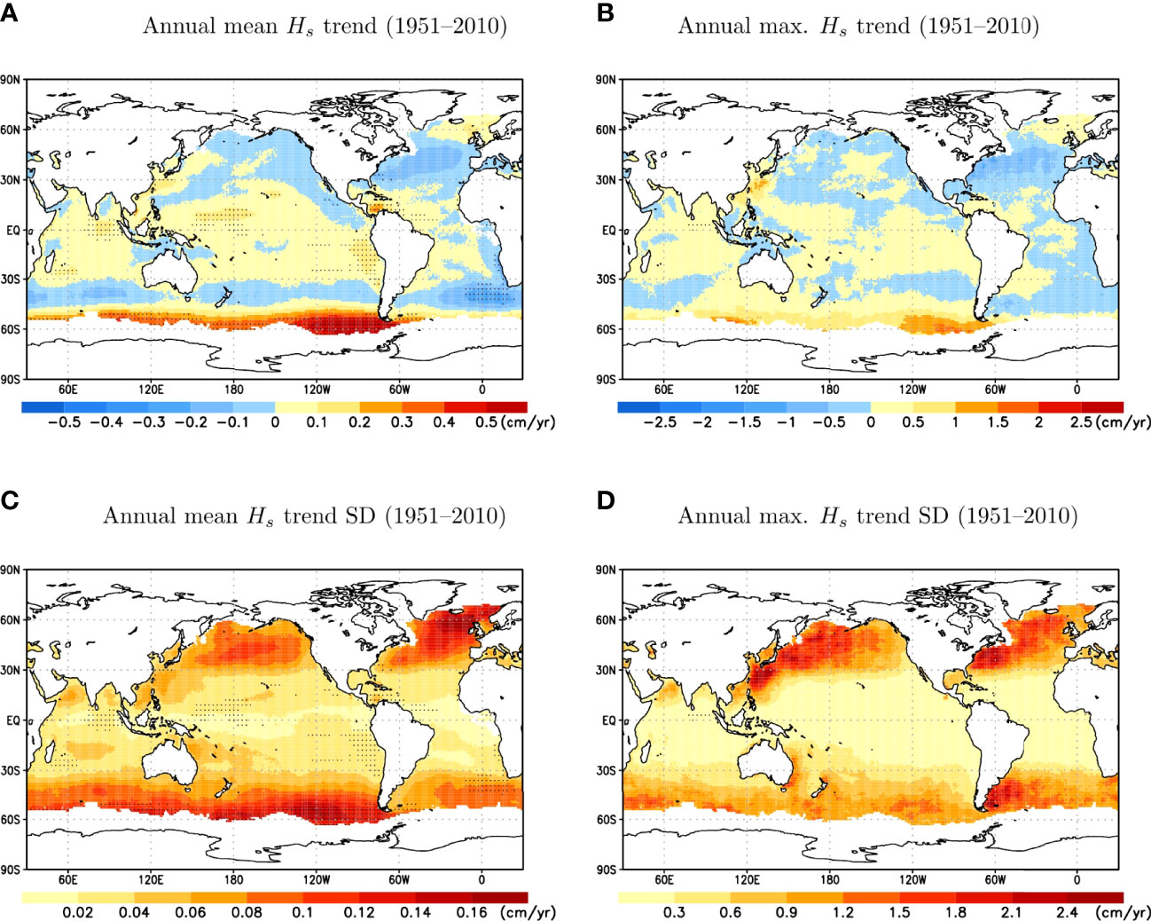
Figure 2 Ensemble average (A, B) and standard deviation (C, D) of the annual mean H_s(A, C) and maximum H_s(B, D) trend (cm/yr) for 1951–2010. Stippling indicates the ensemble mean trend is statistically significant.

Figures 2C, D illustrate the inter-member standard deviation (SD) of the annual mean and maximum H_s trends for the period 1951–2010. For the annual mean H_s, SD is larger in the extra-tropics of both the Northern and Southern Hemisphere, with the largest values being located in the North Atlantic Ocean. For the annual maximum H_s, we see a longitudinal gradient over the extra-tropics, with the larger SD being located in the Western parts of the North Pacific, North Atlantic, and South Atlantic basins. This is arguably related to these areas being more sheltered from swells and therefore more affected by local (more variable) extreme storms than the eastern side of the basin counterpart. Swells likely contribute to lower internal climate variability as they integrate different wave energy systems generated by different atmospheric systems across multiple locations.

It is important to note that the areas identified as statistically significant can differ notably depending on the statistical method used to assess uncertainty. As explained in Section 2.2, here we use a 2-step method that accounts for both inter-run and inter-annual variability, as recommended by the IPCC for assessing robustness. If we use a less conservative approach such as a t-test to determine if the ensemble average trend is statistically different from zero, we obtain significantly larger areas of statistically significant trends that cover most of the domain (see Figure 2 vs Figure S8). For example, in the North Atlantic Ocean, we obtain statistically significant positive trends in its north-east part while the central-west part exhibits a trend that is statistically significant and negative. Note that this t-test only accounts for the trend estimates associated to the individual ensemble members, without considering the inter-annual variability and the statistical significance associated to each individual member.

At regional scale, Figure 3 shows the global and regional ensemble averages of the trends over the period 1951–2100 in the form of a boxplot, along with the 5%, 25%, 50%, 75%, and 95% percentiles of the trend estimates. The corresponding values relative to the 1951–2100 climatological mean are shown in Figure S9. One significant result is that at least 95% of the members exhibit a global positive trend for the annual mean H_s. At regional scale, the 5% percentile of the annual mean H_s trends also exceeds zero in some tropical areas, and in the Southern Hemisphere (WTNP, ETSP, TSIO and SP, see Figure 1). NA is the region with more members exhibiting a negative trend for the annual mean and maximum H_s. For the annual maximum H_s, the inter-member variability increases and a smaller number of areas (TSIO and SP) have at least 95% members exhibiting positive trends. Overall, the areas where the trend estimate is more affected by internal climate variability are the extra-tropical areas, and particularly the Northern Hemisphere extra-tropics (NA and NP), which exhibit larger spread in both trend magnitude (cm/yr, see Figure 3) and percent relative to the 1951–2010 climatology (%/yr, Figure S9).

FIGURE 3

Figure 3 Ensemble average of the regional trend (cm/yr) of the annual mean (A) and maximum (B)H_s averaged over the indicated area (see Figure1), corresponding to the 1951–2010 (black) and 1979–2010 (gray) periods. Dots indicate: ERA5 (blue), ERAint (green) and CFSR (purple) corresponding values for 1979–2010. Box plot illustrates the 2.5%, 25%, 50%, 75% and 97.5% percentiles.

Figure 3 also illustrates how the regional trends for the period 1979–2009 compare to the corresponding values of state-of-the-art reanalysis. As expected, the inter-member variability is larger due to considering a shorter period of time. We observe striking discrepancies between the analyzed NCEP and ECMWF products (CFSR vs. ERA5 and ERAint), which exceed the internal climate variability (as derived from d4PDF-WaveHs). While ERA5 and ERAint simulate positive trends for annual mean H_s over the majority of the regions, CFSR mostly depicts negative trends, which are particularly strong in the Southern Ocean. The corresponding regional average derived from d4PDF-WaveHs typically lies in between the values associated to these reanalyzes products. These discrepancies are also seen in the spatial patterns of the ensemble average trends for both the trend magnitude (cm/yr) and the trend relative to 1979–2009 (%/yr) of the annual mean H_s (Figures S10, S11). ERA5 and ERAint trends are mostly positive (and exceeding 0.5 cm/yr), while the corresponding values of CFSR are mostly negative with a similar amount.

For the regional annual maximum H_s trends, ERA5 and ERAint also simulate larger values than CFSR, often with opposite signs. However, such discrepancies are lower than what is in the annual mean H_s (relative to the d4PDF-WaveHs spread) and, for a few regions (NA, SIO and SA, see Figure 1), they even fall within the internal climate variability simulated by 4PDF-WaveHs. As for the annual mean H_s trend, the corresponding trend maps for the annual maximum H_s (Figures S12, S13) also illustrate disparities among the analyzed products but we find a larger agreement between 4PDF-WaveHs and CFSR, as better captured by the individual runs (Figures S6, S7 vs Figure S12B).

As mentioned in the Introduction, recent studies also found significant discrepancies among modern wave reanalysis datasets. While differences in resolution and wave modelling method configurations can contribute to the differences in trends simulated by different wave climate products analyzed in this study, we argue that the major discrepancies are largely affected by temporal inhomogeneities introduced in assimilated data, in agreement with previous studies (e.g. Aarnes et al., 2015; Stopa et al., 2019; Wohlkand et al., 2019; Sharmar et al., 2020). The comparison among reanalysis products alone seems to indicate that resolution is not a key factor explaining the discrepancies in the trends therein. ERAint (which has the same spatial resolution as 4dPDF-WaveHs) exhibits a trend pattern similar to ERA5 while the latter has significantly higher spatial resolution. Differently, ERA5 and CFSR have contrasting trends while having more similar spatial resolutions. Also, the discrepancies between ERAint/ERA5 and CFSR remain in terms of the relative trend (Figures S12, S13), which is a trend quantity less affected by resolution. The difference between the statistical and the dynamical wave modelling approaches does not seem a key factor in explaining the discrepancies between the trends obtained from 4dPDF-WaveHs and the modern reanalysis either, as we showed how the annual mean and maximum H_s trends of the first run of 4dPDF-WaveHs exhibited similar patterns in comparison to the counterpart simulated by WW3 (Figures S1, S2).

The temporal inhomogeneities present in modern reanalysis can be illustrated with the abrupt changes in tendency and spread seen in the annual mean H_s time series of Figures 4 and 5 (see also Figures S14−S16 for other regions). For example, CFSR, ERAint and ERA5 simulate a global average of the annual mean H_s (Figure 4A) that goes from 2.23 m to 2.53 m in the first half of the reanalysis period, while the range is reduced to 2.28 m to 2.45 m for the second half. This is caused by an abrupt change in tendency starting in the 1990s, which coincides with the start of assimilated wave integrated parameters in the early 1990s, followed by an increase of overall satellite data in the 2000s (Herbach et al., 2020). The global annual maximum H_s (Figure 4B) does not exhibit such an abrupt breakpoint but the model spread also tends to decrease after the 1990s. Overall, we find a better agreement among the annual mean H_s trends simulated by d4PDF-WaveHs and modern reanalysis datasets at global scale. For the global annual maximum H_s, the values simulated by d4PDF-WaveHs (and also CMIP5-HsWang) are lower than those simulated by the reanalysis products. This is mostly caused by an underestimation of the annual maximum H_s in the tropics (see for example the WTNP, ETNP, TNA, WTSP, ETSP, TSA, TSIO regions in Figures S14−16) while there is a good agreement for the annual maximum H_s over the mid to high latitudes (e.g. NP, NA, SP and SA regions, see Figure 5 and Figures S14−S16).

FIGURE 4

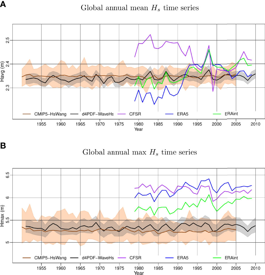
Figure 4 Global time series of the annual mean H_s(A) and annual maximum H_s(B), in m, as derived from d4PDF-WaveHs (black), CMIP5-HsWang (brown), CFSR (purple), ERA5 (blue), ERAint (green). For the d4PDF-WaveHs and CMIP5-HsWang ensembles we show the ensemble mean (thick lines) and the range between the 2.5% and 97.5% percentiles (shaded area).

FIGURE 5

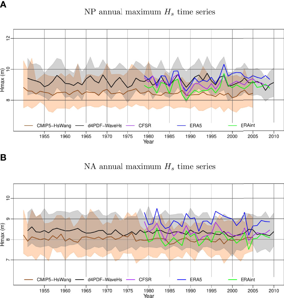
Figure 5 NP (A) and NA (B) time series of the annual maximum H_s, in m, as derived from d4PDF-WaveHs (black), CMIP5-HsWang (brown), CFSR (purple), ERA5 (blue), ERAint (green). For the d4PDF-WaveHs and CMIP5-HsWang ensembles we show the ensemble mean (thick lines) and the range between the 2.5% and 97.5% percentiles (shaded area).

Since modern reanalysis datasets do not seem to be suitable observation proxies for trend analysis, we compare the trends derived from d4PDF-WaveHs with the corresponding values obtained from other model simulations without data assimilation: CMIP5-HsWang and CMIP5-COWCLIP (see Section 2.3). This also allows us to assess the role of the internal climate variability, as estimated from d4PDF-WaveHs, in the context of other sources of uncertainty. In terms of the global annual mean and maximum H_s time series, CMIP5-COWCLIP notably exhibits the largest variability, as expected since this ensemble considers a large variety of wave modelling approaches and configurations (see Figure S17). However, we find that the uncertainty of the global averaged trends (of both annual mean and maximum H_s trends) is fairly similar for the three data products, with significantly overlapping ranges of variability (seeFigure 6andFigure S18). d4PDF-WaveHs tends to have a lower spread, followed by CMIP5-HsWang and CMIP5-COWCLIP, respectively, which might indicate that the global variability induced by climate models is larger than the internal climate variability, and that adding another factor of uncertainty (wave method) further increases the variability, as expected. However, this is not the case for all regions. For example, the North Atlantic annual mean H_s trend variability derived from d4PDF-WaveHs equals the CMIP5-COWCLIP counterpart (while exceeding the CMIP5-HsWang value). In any case, the differences in spread are mild and could be caused by the difference in sampling space (different ensemble sizes). For example, Figure S19 shows the spread of global trends that would be obtained from 20- and 48-size sub-ensembles randomly sampled from d4PDF-WaveHs, in comparison to the original 100-size ensemble.

FIGURE 6

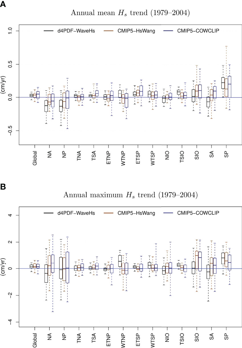
Figure 6 Ensemble average of the regional trend (cm/yr) of the annual mean (A) and maximum (B)H_s averaged over the indicated areas (see Figure 1) as derived from d4PDF-WaveHs (black), CMIP5-HsWang (brown) and CMIP5-COWCLIP (dark blue) for the 1979–2005 (see Section 2). Box plot illustrates the 2.5%, 25%, 50%, 75% and 97.5% percentiles.

Finally, we addressed the risk of using a single member to assess trends. In some areas of the Southern Ocean, there is a likelihood of up to 50% to miss the statistically significant strong positive trend that is clearly shown by the ensemble average for the annual mean H_s (Figure 7A). The chances to get the same trend sign (regardless of the significance) are however larger in those areas. In contrast, the likelihood to obtain the same trend sign decreases to about 50% in the North Atlantic (Figure 7B) as the wave climate in this region has larger internal climate variability, for which individual members can predict either positive or negative trends locally (Figures S4, S5). However, the results also show that, for the annual mean H_s, it is very unlikely for an individual member to have a statistically significant trend of the opposite sign to the ensemble average trend (Figure 7C). This only occurred in at most 5 out of the 100 members over a few scattered areas at the mid to high latitudes.

FIGURE 7

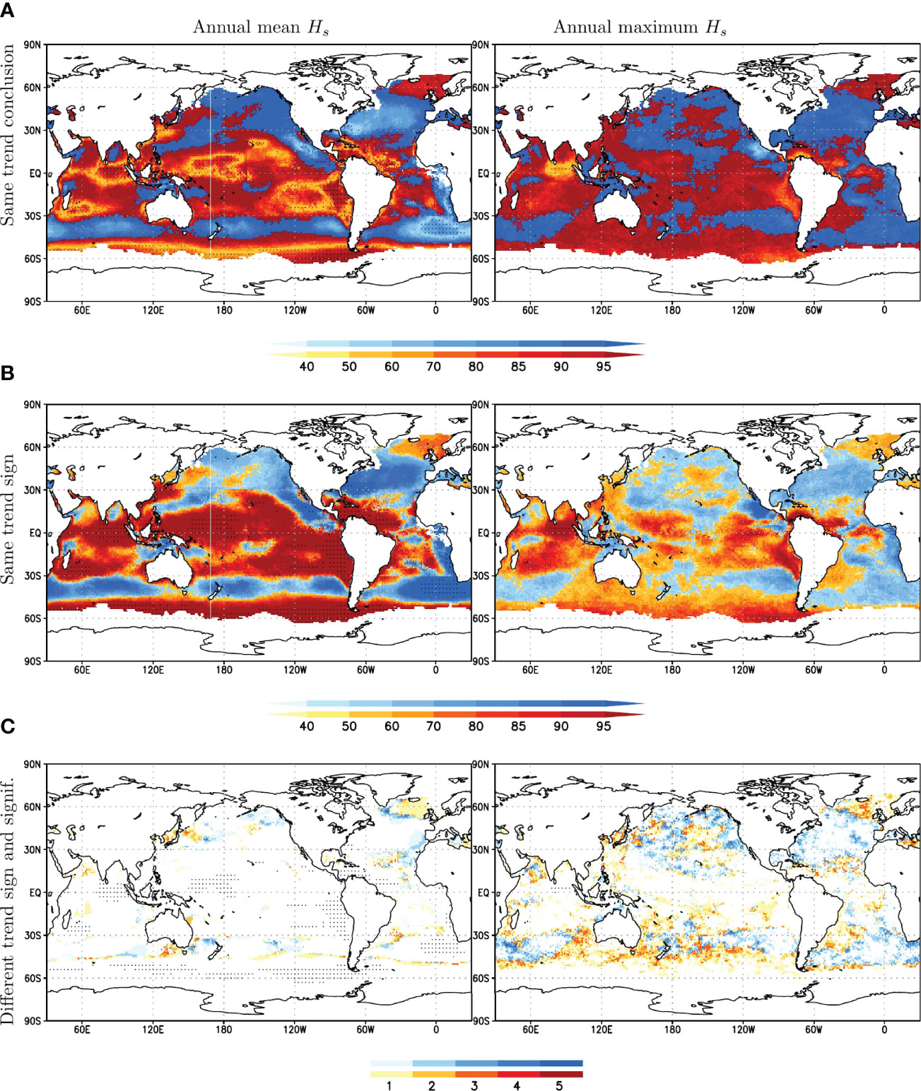
Figure 7 Fraction of ensemble members (%) with the same trend conclusion (A), the same trend sign (B) and different trend sign that is statistically significant (C), as compared to the ensemble average for the annual mean H_s (left) and the annual maximum H_s (right) (see Section 2.2 for more details). Warm(cold) shades indicate the ensemble mean trend is positive(negative). Stippling indicates the ensemble mean trend is statistically significant.

For the annual maximum H_s, the chances to get the same trend conclusion are very high, especially for the areas with positive trends (Figure 7A). This can be explained by the low statistical significance found in most of the members (using the more restrictive method to assess robustness, see Section 2.2), but there is a larger disagreement (>50% runs) in simulating the same trend sign (Figure 7B). Also, the areas where up to 5 individual ensemble members might simulate a statistically significant trend of the opposite sign to that of the ensemble average are more abundant and cover most of the mid and high latitudes (Figure 7C). The corresponding ensemble average of the annual mean and maximum Hs trends are shown in Figures S20andS21.

The same analysis performed for sub-ensembles with varying ensemble size reveals that, as expected, the required ensemble size to replicate the results obtained from the whole 100-member ensemble depends on the H_s statistic and the region in question (see Figures S22−25). For example, for the annual mean H_s, the areas of trend conclusion disagreement (which considers both trend sign and significance) over the Southern Ocean, notably shrink when we consider sub-ensembles with size close to 20 members (Figure S22). Differently, if we want to simulate the same annual mean H_s trend sign over the North Atlantic, a 10-size ensemble seems to be sufficient (Figure S23). For the annual maximum H_s we would generally require larger ensembles to obtain the same trend sign (for example close to 40 for the North Atlantic Ocean, see Figure S25), as expected due to the larger uncertainty associated with simulating extremes. Overall, at global scale we argue that a trend assessment using a SMILE-based ensemble with size from 10 to 20 would reduce significantly the likelihood for an erroneous trend assessment result.

4 Discussion

We have used the d4PDF-WaveHs, the first SMILE-based large wave height ensemble to assess the effects of internal climate variability on trend assessment results. d4PDF-WaveHs consists of 100 ensembles of 60-year historical H_s simulations (1951–2010). In this study, we focused on the analysis of the annual mean and maximum H_s trends and the role that the internal variability plays in their assessment; but this dataset can be further exploited in future studies to investigate the role of internal climate variability on other target quantities, such as low-frequency H_s extremes.

The trends obtained from d4PDF-WaveHs are also compared to those derived from modern reanalysis datasets and from climate model simulations. This is of particular relevance given the notable discrepancies among reanalysis datasets in recent studies (Stopa et al., 2019; Sharmar et al., 2020). Moreover, this study also contributes to improve the current understanding of the internal wave climate variability, which is a key factor among other relevant sources of uncertainty affecting wave simulations (Morim et al., 2019).

We found a clear and statistically significant positive trend for the annual mean H_s over the Southern Ocean exceeding 0.5 cm/yr in some areas. Statistically positive trends with a lower intensity (up to 0.3 cm/yr) were also seen for tropical areas. Over the North Pacific and Atlantic Oceans, the averaged trends are not statistically significant, which is caused by the large inter-annual variability in these areas, where individual ensemble-members might simulate opposite trends although most of the simulations show a negative regional trend. The annual maximum H_s trends show a similar spatial pattern but results are not statistically significant. Significance here is assessed with a two-step method that accounts for both the inter-annual variability in each individual member as well as the variability among members, as recommended by the IPCC to assess robustness.

The results here provide more evidence that modern reanalysis datasets are not suitable observation proxies to study historical wave height trends due to their temporal inhomogeneities. The main reason is arguably the increasing amount and type of available observations used in data asimilation, which coincides with breakpoints that can be visually identified in the annual mean H time series. In most regions, ERA5 and ERAint simulate positive trends while CFSR simulate negative trends, and the results simulated by d4PDF-WaveHs fall in between these two family products. The discrepancies are more notable for the annual mean H_s than for the annual maximum H_s, which seems to be less affected by temporal inhomogeneities. While differences in resolution and wave modelling methodologies might contribute to add variability in the assessment of the wave climatology (particularly the extremes), the temporal inhomogenity induced by data assimilation is arguably the main factor leading to the major discrepancies observed for the annual mean and maximum H_s trends.

Our results show that there is a non-negligible probability to miss-assess trends when using a single realization (member). Although we would likely detect the strong positive trend in the annual mean H_s over Southern Ocean with just one member, we could mis-estimate their spatial extension and therefore mis-assess the trend locally (in up to 50% of the ensemble members). For the annual maximum H_s, there is a larger uncertainty; opposite trends are simulated by the individual members, particularly in the North Pacific and North Atlantic oceans. However, it is unlikely to obtain an individual trend that is fundamentally opposite of the corresponding ensemble average. To reduce the risk to miss-assess trends at global scale, it would be necessary to use at least 10 members. However, an optimal size depends on the statistic quantity and region analyzed.

This study also shows that, despite climate model variability leading to a large uncertainty for the assessment of the annual mean and maximum H_s time series, the role of the internal climate variability in the resulting trends is comparable to the uncertainty derived from climate models and wave methods. However, this comparison is challenging given the uneven sampling of the uncertainty factors in the available datasets. Typically, ensembles that consider different climate models have a limited amount of realizations and SMILEs are based on a single climate model by definition. Future studies with climate datasets that better represent the whole spectrum of uncertainty would likely help understand better the contribution of these uncertainty factors.

The dataset and analysis presented in this study bring significant insight into the role of internal variability in the context of the wave height trend assessment. However, results are based on a single-model ensemble and therefore rely on the ability of this particular climate model to replicate the internal climate variability. It would be ideal to perform a similar analysis with other SMILE-based large wave ensembles that consider other climate models in order to derive more robust conclusions that are not specific to a particular climate model. Additionally, results rely on the performance of the statistical wave modelling approach to obtain H_s. In this regard, we plan to re-calibrate the statistical wave modelling approach with a higher resolution product (e.g. ERA5) which might improve the underestimation seen in the tropics, and better capture the storms with sharp SLP gradients. Moreover, to fully address the main wave-driven impacts, we need to also consider and analyze other wave variables such as wave period and wave direction.

Data Availability Statement

The raw data supporting the conclusions of this article will be made available by the authors, without undue reservation.

Author Contributions

MC-P wrote the manuscript. MC-P and XW co-designed/led the study. YF contributed to the statistical data analysis. XW conceived and produced the d4PDF-WaveHs dataset with the Disaster Prevention Research Institute (DPRI) of Kyoto University providing funding support for her two-month sabbatical at DPRI hosted by NM. YF, RC, NM and TS contributed to the production of the d4PDF-WaveHs dataset. NM and TS provided the d4PDF atmospheric data and WW3 wave simulations used for validation. All authors contributed to manuscript revision, and approved the submitted version.

Funding

The Disaster Prevention Research Institute (DPRI) of Kyoto University provided funding support (including roundtrip airfare) for XW’s two-month sabbatical at DPRI 29L01.

Conflict of Interest

The authors declare that the research was conducted in the absence of any commercial or financial relationships that could be construed as a potential conflict of interest.

Publisher’s Note

All claims expressed in this article are solely those of the authors and do not necessarily represent those of their affiliated organizations, or those of the publisher, the editors and the reviewers. Any product that may be evaluated in this article, or claim that may be made by its manufacturer, is not guaranteed or endorsed by the publisher.

Acknowledgments

This study utilized the d4PDF, which was produced using the Earth Simulator as “Strategic Project with Special Support” of JAMSTEC in cooperation with the Program for Risk Information on Climate Change (SOUSEI), TOUGOU, the Social Implementation Program on Climate Change Adaptation Technology (SI-CAT), which all were sponsored by the Ministry of Education, Culture, Sports, Science and Technology of Japan (MEXT)Disaster Prevention Research Institute (DPRI) funding number is 29L01.

Supplementary Material

The Supplementary Material for this article can be found online at: https://www.frontiersin.org/articles/10.3389/fmars.2022.847017/full#supplementary-material

References

Aarnes O., Abdalla S., Jean-Raymond B., Breivik O. (2015). Marine Wind and Wave Height Trends at Different Era-Interim Forecast Ranges. J. Climate 28, 819–837. doi: 10.1175/JCLI-D-14-00470.1

CrossRef Full Text | Google Scholar

Box G., Cox D. (1964). An Analysis of Transformation (With Discussion). J. R. Stat. Soc. 26, 211–246.

Google Scholar

Cavaleri L., Fox-Kemper B., Hemer M. (2012). Wind Waves in the Coupled Climate System. Bullet. Am. Meteorolog. Soc. 93, 1651–1661. doi: 10.1175/BAMS-D-11-00170.1

CrossRef Full Text | Google Scholar

Dee D.P., Uppala S.M, Simmons A.J, Berrisford P, Poli P, Kobayashi S., et al (2011). The ERA-Interim Reanalysis: Configuration and Performance of the Data Assimilation System. Quaterly. J. R. Meteorolog. Soc. 137, 553-597. doi: 10.1002/qj.828

CrossRef Full Text | Google Scholar

Dodet G., Piolle J.-F., Quilfen Y., Abdalla S., Accensi M., Ardhuin F., et al (2020). The Sea State CCI Dataset V1: Towards a Sea State Climate Data Record Based on Satellite Observations. Earth Syst. Sci. Data 12, 1929–1951. doi: 10.5194/essd-12-1929-202

CrossRef Full Text | Google Scholar

Grifoll M., Martínez de Osés F., Castells M. (2018). Potential Economic Benefits of Using a Weather Ship Routing System at Short Sea Shipping. WMO. J. Maritime. Affairs. 17, 195–211. doi: 10.1007/s13437-018-0143-6

CrossRef Full Text | Google Scholar

Griggs G., Reguero B. (2021). Coastal Adaptation to Climate Change and Sea-Level Rise. Water 13, 2151. doi: 10.3390/w13162151

CrossRef Full Text | Google Scholar

Gudmestad O. T. (2020). Modelling of Waves for the Design of Offshore Structures. J. Mar. Sci. Eng. 8, 293. doi: 10.3390/jmse8040293

CrossRef Full Text | Google Scholar

Herbach H, Bell B., Berridford P., Hirahara S, Horányi A., Muñoz-Sabater J., et al (2020). The ERA5 Global Reanalysis. Quaterly. J. R. Meteorolog. Soc. 146, 1999–2049. doi: 10.1001/qj.3803

CrossRef Full Text | Google Scholar

Huppert K. L., Perron J. T., Ashton A. D. (2020). The Influence of Wave Power on Bedrock Sea-Cliff Erosion in the Hawaiian Islands. Geology 48, 499–503. doi: 10.1130/G47113.1

CrossRef Full Text | Google Scholar

International Organization for Standarization (2007). ISO 21650: Actions From Waves and Currents on Coastal Structures (ISO/TC 98/SC 3, ICS 91.080.01). Available at: https://www.iso.org/standard/35955.html

Google Scholar

IPCC (2013). “Climate Change 2013,” in The Physical Science Basis. Contribution of Working Group I to the Fifth Assessment Report of the Intergovernmental Panel on Climate Change, vol. 1535 . Eds. Stocker T. F., Qin D., Plattner G.-K., Tignor M., Allen S. K., Boschung J., Nauels A., Xia Y., Bex V., Midgley P. M. (Cambridge, United Kingdom and New York, NY, USA: Cambridge University Press).

Google Scholar

Ishii M., Mori N. (2020). d4PDF: Large-Ensemble and High-Resolution Climate Simulations for Global Warming Risk Assessment. Prog. Earth Planet. Sci. 7. doi: 10.1186/s40645-020-00367-7

CrossRef Full Text | Google Scholar

Kirchmeier-Young M., Zhang X, Wan H. (2021): Climate Change Attribution With Large Ensembles. EGU General Assembly 2021 EGU21–3404. doi: 10.5194/egusphere-egu21-3404

Google Scholar

Maher N., Milinski S., Ludwig R. (2021). Large Ensemble Climate Model Simulations: Introduction, Overview, and Future Prospects for Utilizing Multiple Types of Large Ensemble. Earth System. Dynamics. 12, 401–418. doi: 10.5194/esd-12-401-2021

CrossRef Full Text | Google Scholar

Mei W., Kamae Y., Xie S.-P., Yoshida K. (2019). Variability and Predictability of North Atlantic Hurricane Frequency in a Large Ensemble of High-Resolution Atmospheric Simulations. J. Climate 32, 3153–3167. doi: 10.1175/JCLI-D-18-0554.1

CrossRef Full Text | Google Scholar

Melet A., Almar R., Hemer M., Le Cozannet G., Ruggiero P. (2020). Contribution of Wave Setup to Projected Coastal Sea Level Changes. J. Geophys. Res. Oceans. 125, e2020JC016078. doi: 10.1029/2020JC016078

CrossRef Full Text | Google Scholar

Melet A., Meyssignac B., Almar R., Le Cozannet G. (2018). Under-Estimated Wave Contribution to Coastal Sea-Level Rise. Nat. Climate Change 8,234–139. doi: 10.1038/s41558-018-0088-y

CrossRef Full Text | Google Scholar

Milinski S., Maher N., Olonscheck D. (2020). How Large Does a Large Ensemble Need to be? Earth Syst. Dynamics. 11, 885–901. doi: 10.5194/esd-11-885-2020

CrossRef Full Text | Google Scholar

Mizuta R., Murata A., Ishii M., Shiogama H., Hibino K., Mori N., et al. (2017). Over 5,000 Years of Ensemble Future Climate Simulations by 60-Km Global and 20-Km Regional Atmospheric Models. Bull. Am. Meteorolog. Soc. 98, 1383–1398. doi: 10.1175/BAMS-D-16-0099.1

CrossRef Full Text | Google Scholar

Mizuta R., Yoshimura H., Murakami H., Matsueda M., Endo H., Ose T., et al. (2012). Climate Simulations Using Mri-Agcm3.2 With 20-Km Grid. J. Meteorolog. Soc. Japan. Ser. II 90, 233–258. doi: 10.2151/jmsj.2012-A12

CrossRef Full Text | Google Scholar

Morim J., Hemer M., Andutta F., Shimura T., Cartwright N. (2020). Skill and Uncertainty in Surface Wind Fields From General Circulation Models: Intercomparison of Bias Between AGCM, AOGCM and ESM Global Simulations. Int. J. Climatol. 40, 2659–2673. doi: 10.1002/joc.6357

CrossRef Full Text | Google Scholar

Morim J., Hemer M., Wang X. L., Cartwright N., Trenham C., Semedo A., et al. (2019). Robustness and Uncertainties in Global Multivariate Wind-Wave Climate Projections. Nat. Climate Change 9, 711–718. doi: 10.1038/s41558-019-0542-5

CrossRef Full Text | Google Scholar

Reguero B. G., Nigo L., Losada I., Méndez F. J. (2019). A Recent Increase in Global Wave Power as a Consequence of Oceanic Warming. Nat. Commun. 10, 205. doi: 10.1038/s41467-018-08066-0

PubMed Abstract | CrossRef Full Text | Google Scholar

Saha S., Moorthi S., Wu X., Wang J., Nadiga S., Tripp P., et al. (2014). The NCEP Climate Forecast System Version 2. J. Climate 146, 2185–2208. doi: 10.1175/JCLI-D-12-00823.1

CrossRef Full Text | Google Scholar

Santos V. M., Casas-Prat M., Poschlod B., Ragno E., van den Hurk B., Hao Z., et al. (2021). Statistical Modelling and Climate Variability of Compound Surge and Precipitation Events in a Managed Water System: A Case Study in the Netherlands. Hydrol. Earth System. Sci. 25, 3595–3615. doi: 10.5194/hess-25-3595-2021

CrossRef Full Text | Google Scholar

Sharmar V. D., Markina M. Y., Gulev S. K. (2020). Global Ocean Wind-Wave Model Hindcasts Forced by Different Reanalyzes: A Comparative Assessment. J. Geophys. Res. Oceans. 126, e2020JC016710. doi: 10.1029/2020JC016710

CrossRef Full Text | Google Scholar

Shimura T., Nobuhito M. (2019). High-Resolution Wave Climate Hindcast Around Japan and its Spectral Representation. Coast. Eng. 151, 1–9. doi: 10.1016/j.coastaleng.2019.04.013

CrossRef Full Text | Google Scholar

Song Z., Bao Y., Zhang D., Shu Q., Song Y., Qiao F. (2021). Centuries of Monthly and 3-Hourly Global Ocean Wave Data for Past, Present, and Future Climate Research. Nat. Sci. Data 7. doi: 10.1038/s41597-020-0566-8

CrossRef Full Text | Google Scholar

Stive M. J., Aarninkhof S. G., Hamm L., Hanson H., Larson M., Wijnberg K. M., et al. (2002). Variability of Shore and Shoreline Evolution. Coast. Eng. 47, 211–235. doi: 10.1016/S0378-3839(02)00126-6

CrossRef Full Text | Google Scholar

Stopa J. E., Ardhuin F., Stutzmann E., Lecocq T. (2019). Sea State Trends and Variability: Consistency Between Models, Altimters, Buoys and Sesimic Dat-2016). J. Geophys. Res. Oceans 124, 2923–3940. doi: 10.1029/2018JC014607

CrossRef Full Text | Google Scholar

Swart N. C., Fyfe J. C., Hawkins E., Kay J. E., Jahn A. (2015). Influence of Internal Variability on Arctic Sea-Ice Trends. Nat. Climate Change 5, 86–89. doi: 10.1038/nclimate2483

CrossRef Full Text | Google Scholar

vonStorch H., Zwiers F. (1999). Statistical Analysis in Climate Research (Cambridge, United Kingdom: Cambridge University Press).

Google Scholar

Wang X. L., Feng Y., Swail V. R. (2012). North Atlantic Wave Height Trends as Reconstructed From the Twentieth Century Reanalysis. Geophys. Res. Lett. 39, L18705. doi: 10.1029/2012GL053381

CrossRef Full Text | Google Scholar

Wang X. L., Feng Y., Swail V. R. (2014). Changes in Global Ocean Wave Heights as Projected Using Multimodel Cmip5 Simulations. Geophys. Res. Lett. 41, 1026–1034. doi: 10.1002/2013GL058650

CrossRef Full Text | Google Scholar

Wang X. L., Feng Y., Swail V. R. (2015). Climate Change Signal and Uncertainty in CMIP5-Based Projections of Global Ocean Surface Wave Heights. J. Geophys. Res. Oceans 120 , 3859-3871. doi: 10.1002/2015JC010699

CrossRef Full Text | Google Scholar

Wang X. L., Swail V. R. (2001). Changes of Extreme Wave Heights in Northern Hemisphere Oceans and Related Atmospheric Circulation Regimes. J. Climate 14, 2204–2221. doi: 10.1175/1520-0442(2001)014<2204:COEWHI>2.0.CO;2

CrossRef Full Text | Google Scholar

Wohlkand J., Omrani N., Witthaut D., Keenlyside N. (2019). Inconsistent Wind Speed Trends in Current Twentieth Century Reanalyses. J. Geophys. Res. Atmos. 124, 1931–1940. doi: 10.1029/2018JD030083

CrossRef Full Text | Google Scholar

Yang S., Oh J.-H. (2020). Effects of Modes of Climate Variability on Wave Power During Boreal Summer in the Western North Pacific. Nat. Sci. Rep. 10, 517. doi: 10.1038/s41598-020-62138-0

CrossRef Full Text | Google Scholar