Sea Levels Dynamical Downscaling and Climate Change Projections at the Uruguayan Coast

This work implements a dynamical downscaling approach, based on a set of nested two-dimensional hydrodynamic models, to quantify the expected changes in the total sea level climate and its components for the Uruguayan coast, using surface wind and sea level pressure projections from global climate models generated during the Phase 5 of the Coupled Models Inter-Comparison Project, considering three time horizons: historical period (1986-2005), short term (2027-2045) and long term (2082-2100), and the future scenarios RCP 4.5 and RCP 8.5. It is concluded that the main contribution to the projected changes in the area is the regional mean sea level rise, followed in importance by the effect that the increase in the water depth has on the amplitude of the tidal components. Moreover, it is concluded that changes in the meteorological residuals (or surges), associated with potential changes in the atmospheric circulation patterns, are negligible in the study area. The obtained results reinforce the need to resort to dynamic downscaling for projecting total sea level changes in areas characterized by wide and shallow continental shelfs and estuaries, as this approach allows to resolve the interactions that may arise between tides, surges and the mean sea level rise, something that cannot addressed with an approach based solely on statistical downscaling.

1 Introduction

The planning of coastal adaptation measures to climate change requires projections of the changes that are expected to occur in the maritime agents (i.e. waves and sea level) in the future under different scenarios and for different time horizons. There are several studies aimed at quantifying future changes in the waves and sea level climates at global or regional scales (e.g. Hemer et al., 2015; Vousdoukas et al., 2016; Camus et al., 2017; Casas-Prat et al., 2017; Wandres et al., 2017; Meucci et al., 2020). All these studies share a common line of work where results from global climate models (GCM), such as surface winds and sea level pressures (SLP), are used to project changes in the variables of interest in a certain domain, resorting to one of the two methodologies available to this end, known as statistical and dynamic downscaling.

Statistical downscaling methods are based in training statistical models that relate predictor (winds and SLP) and predictand (waves and/or sea levels) variables. These methods are inexpensive from a computational point of view, which makes it possible to use a large number of GCMs, allowing to improve the quantification of the uncertainty involved and the consensus of the projected changes (Perez et al., 2015). In fact, the studies using statistical downscaling methods usually use all GCM results available (e.g. Wang et al., 2014; Camus et al., 2017). On the other hand, dynamic downscaling is based on the use of physics-based numerical models that are forced with wind and SLP fields time series obtained from the GCM, resulting in high computational costs and, also, in more demanding requirements in terms of spatial and temporal resolution of the GCM used to force the models (e.g. Vousdoukas et al., 2016).

When looking at changes in the sea level, an advantage of the dynamical downscaling over the statistical downscaling is that the use of physic-based numerical models allows for considering the non-linear interactions between the different components that make up the total sea level and its change, namely: mean sea level rise, astronomical tides (or tides) and meteorological residuals (or surges). Unlike dynamical downscaling, the statistical downscaling approach can only determine changes directly associated with changes in atmospheric patterns (see e.g. Camus et al., 2014).

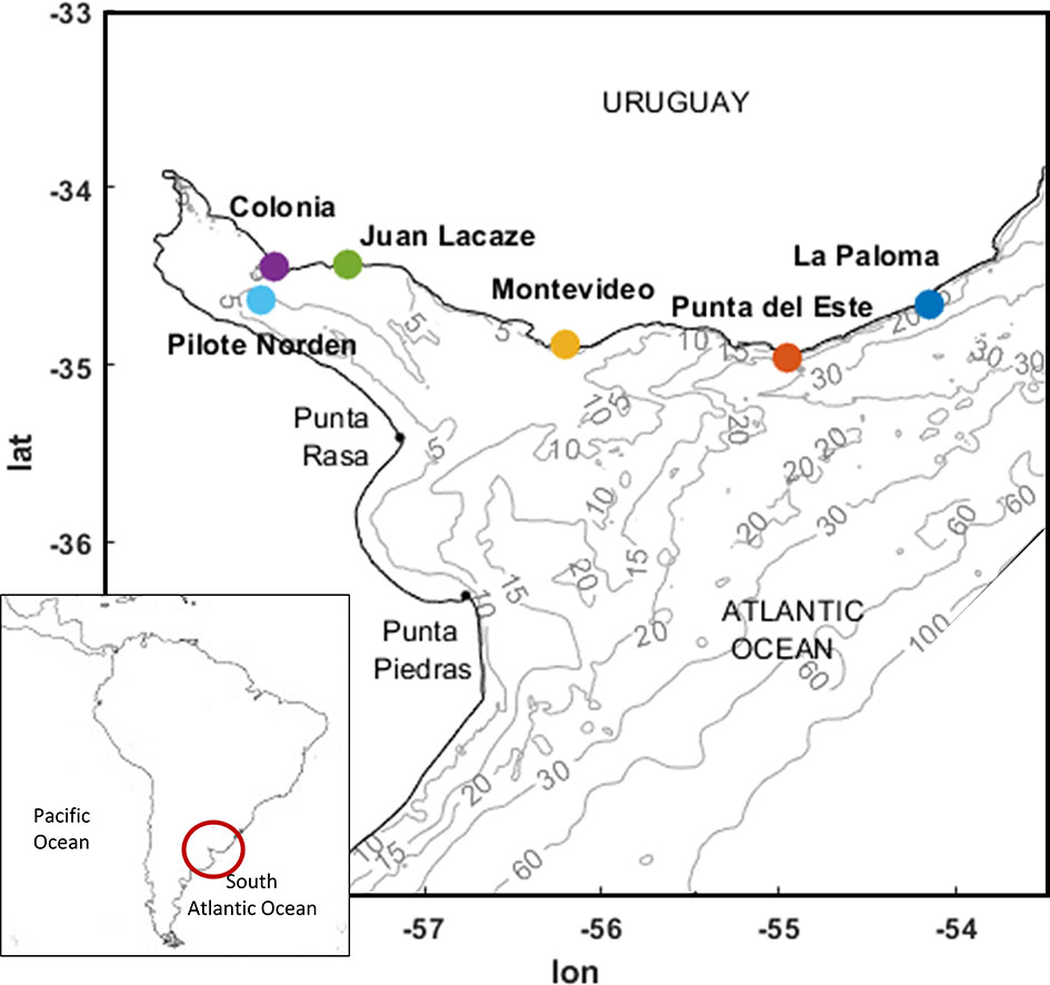
Uruguay has more than 600 km of coast, encompassing both the Río de la Plata estuary and the Atlantic Ocean (Figure 1). Along the coast, meteorological residuals and astronomical tides have the same order of magnitude and are important components of the total sea level (Santoro et al., 2013). The main component of the astronomical tide is M2, with amplitudes of up to 15 cm, followed by component O1 in most of the coast (Fernández & Piedra-Cueva, 2011). Regarding the variability of the M2 amplitude along the coast, there is a tendency of higher amplitudes around Colonia and Montevideo, and lower amplitudes between these and towards the ocean. Studies based on in situ measured sea level data showed that the magnitude of the meteorological residuals (or surges) decrease from the inner part of the estuary towards the ocean (Fossati et al., 2013; Santoro et al., 2013).

FIGURE 1

Figure 1 Study area and in-situ measurements stations along with the bathymetry of the area.

Despite the importance of specifically knowing how total sea level will change along the Uruguayan coast, there are few studies in relation to this. While there are global studies about mean sea level change projections (e.g. IPCC, 2013; Slangen et al., 2014; Carson et al., 2016), there are no global or regional studies that determine the change in the total sea level climate for this zone.

The objective of this work is to quantify the expected changes in the total sea level climate and its components for the Uruguayan coast, using surface wind and SLP projections from GCM generated during the Phase 5 of the Coupled Models Inter-Comparison Project (CMIP5) (Taylor et al., 2012) in the framework of the WRCP (World Climate Research Program), which are presented in the IPCC fifth report (IPCC, 2013). At the moment, the latest report published by the IPCC is the AR6 (only draft, final publication is expected on September 2022) where the CMIP6 (Eyring et al., 2016) is presented, providing the state of the art climate models; in addition, the Special Report on the Ocean and Cryosphere in a Changing Climate (IPCC, 2019) brings together recent research regarding sea level projections. Nevertheless, at the time of initiating this work only information from IPCC AR5 was available, so this is the one used. Three time horizons are considered: historical period (1986-2005), short term (2027-2045) and long term (2082-2100), and two future scenarios RCP 4.5 and RCP 8.5 (Moss et al., 2010). Given characteristics of the continental shelf and of the Río de la Plata estuary (Figure 1), it is expected that non-linear interactions between sea level rise and tides and surges would play a significant role in the estimation of projected changes, so a dynamic downscaling scheme is adopted in this work.

The rest of the document is organized as follows. Sections 2 and 3 describes the methodology and the data used in this study. Obtained results are presented in section 4 and discussed in section 5, while section 6 summarizes the main conclusions.

2 Methods

2.1 General Methodology

To obtain sea level projections in the study area, a dynamic downscaling methodology is adopted, based on the implementation of two nested hydrodynamic models. The nested models are called regional and local model, and are forced by the inflows from the tributaries of the Río de la Plata estuary, surface winds and SLP, and tides at its outer oceanic boundaries.

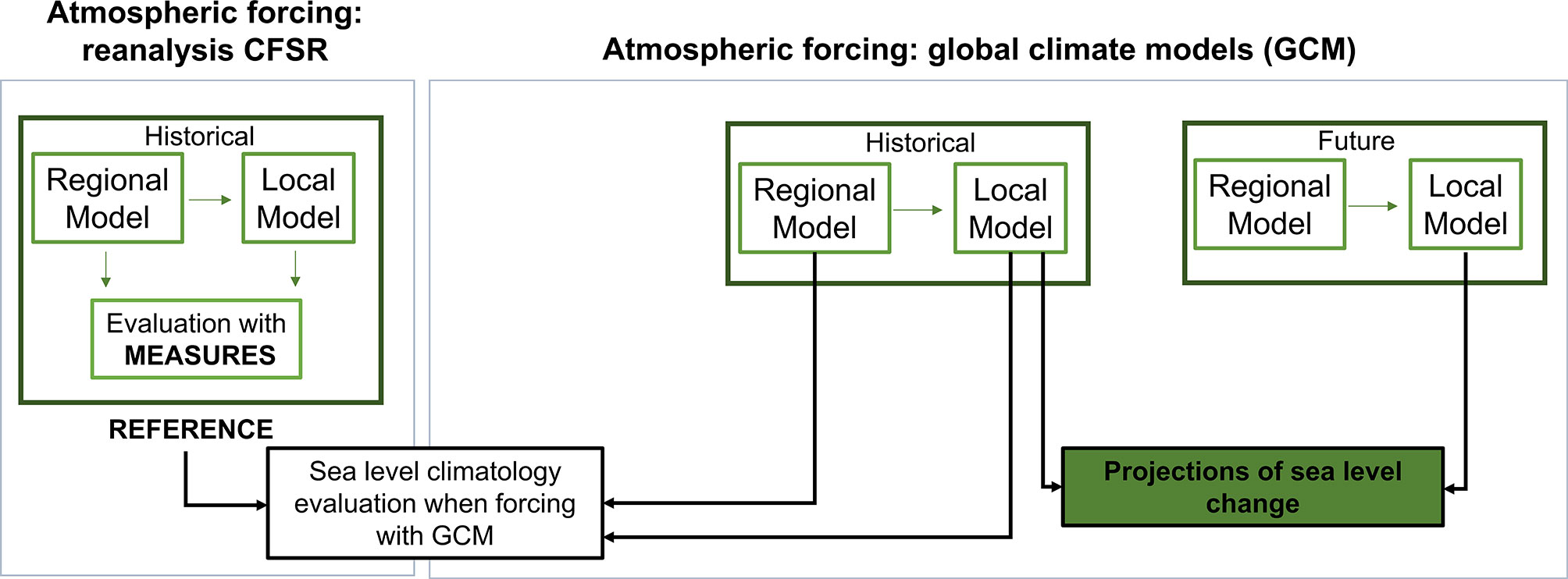
To determine the future sea level climate, the hydrodynamic models are forced with the wind and SLP projections of the GCMs listed in Table 3. Results are obtained for three time-horizons: historical, short term (2027-2045) and long term (2082-2100); and for two representative concentration pathways scenarios: RCP 4.5 and RCP 8.5. Figure 2 shows an outline of the methodology. On the one hand, the models are forced with winds and SLP from the CFSR reanalysis (Saha et al., 2010). Sea level time series obtained with this forcing are validated using measured data to later be considered as the ground true (Figure 2, left panel). On the other hand, models are forced with GCM winds and SLP for both the historical period and the future periods. First, results from the historical period are used to evaluated whether the models correctly represent the sea level climate in the study area when forced with GCMs. Then, changes in the sea level climate are quantified by comparing historical and future periods for each GCM (Figure 2, right panel).

FIGURE 2

Figure 2 Flowchart representing general methodology.

2.2 Hydrodynamic Models Setup

Hydrodynamic modeling is carried out by means of two nested numerical models. Figure 3 shows the domains used in the two models, along with a detail of the inner part of the Río de la Plata estuary.

FIGURE 3

Figure 3 Nested hydrodynamic models scheme used in this study.

The first model encompasses the domain comprised by the South Atlantic Ocean (regional model; Figure 3, left panel), and is forced by astronomical tides at the ocean boundaries, average inflows from the Paraná and Uruguay rivers, and by surface winds and SLP in the free surface. In particular, the astronomical tide is imposed at the ocean boundaries as the superposition of 13 tidal components (M2, N2, S2, K2, 2N2, O1, Q1, K1, P1, Mf, Mm, Mtm, MSqm) obtained from FES2004 global ocean tide atlas (Lyard et al., 2006). The objective of the regional model is to generate the total sea levels time series to be imposed at the oceanic boundaries of the local model (Figure 3; central panel). The regional model is based on MOHID (Mateus and Neves, 2013) and was previously calibrated and validated for this domain (Martínez et al., 2015; Jackson et al., 2021). The most relevant characteristics of its implementation are presented in Table 1.

TABLE 1

Table 1 Features of the setup for both regional and local hydrodynamic models.

The local model is an implementation of TELEMAC-MASCARET (Hervouet, 2007), in its 2D version, to a domain that includes the estuary of the Río de la Plata and its continental shelf (Figure 3, central panel). TELEMAC has been successfully applied in several estuarine dynamics studies (Briere et al., 2007; Jones and Davies, 2008; Guillou & Chapalain, 2012; Huybrechts et al., 2012; Huybrechts & Villaret, 2013; Luo et al., 2013; Sathish Kumar & Balaji, 2015). The vertically integrated two-dimensional hydrodynamic TELEMAC-2D model solves the momentum and continuity equations using finite elements on unstructured meshes. The equations are simplified assuming incompressible fluid, vertical homogeneity, and hydrostatic pressure distribution. The model is forced by surface winds and SLP on the free surface, mean inflows from the Uruguay, Paraná and Santa Lucía rivers (Figure 3, right panel), and from the sea level time series coming from the regional model at the open oceanic boundaries. The time step used for running the model is 60 seconds and results are saved at every node of the mesh every 1 hour. Table 1 summarizes most relevant characteristics of the implementation of the local model.

2.3 Calibration and Validation of the Local Model

The calibration of the model was carried out using data measured during the period 1985 to 2005, forcing the models with the CFSR reanalysis, varying the Manning number and testing different formulations for the wind shear stress. More than 40 calibration simulations were carried out, comparing the obtained results against sea levels measured at 3 stations on the Uruguayan coast, namely: La Paloma, Montevideo and Colonia (see Figure 1).

Validation is performed by comparing the results obtained with the calibrated model and the sea level data measured at the 6 stations shown in Figure 1. The goodness of the model is analyzed by estimating bias (BIAS), mean square error (RMSE) and correlation coefficient (r) at each station, as expressed by equations 1, 2 and 3 respectively,

$\begin{array}{ll}BIAS=\overline{y_m-y_o}& \text{Equation 1}\end{array}$

$\begin{array}{ll}RMSE=\sqrt{\overline{{(y_m-y_o)}^2}}& \text{Equation 2}\end{array}$

$\begin{array}{ll}R=\frac{\Sigma (y_m-\overline{y_m})-(y_o-\overline{y_o})}{\sqrt{\Sigma {(y_m-\overline{y_m})}^2}\sqrt{\Sigma {(y_o-\overline{y_o})}^2}}& \text{Equation 3}\end{array}$

where y_m refers to the modeled data and y_o to the measured (observed) data. In addition, scatter diagrams are presented for total sea level and for the meteorological residual, showing data density according to a color scale, superimposed by a quantile-quantile plot (25 quantiles are considered, evenly spaced on the Gumbel scale, between 0.001 and 0.999). Once validated, results of the model are considered the ground true for subsequent analyzes.

2.4 Projections of Change in Sea Level Climate

The analysis of the sea level projections obtained by forcing the numerical models with the GCM is carried out focusing on different spatial and temporal scales, using a series of evenly spaced nodes located along the Uruguayan coast, from Conchillas to Chuy (see e.g. Figure 8A).

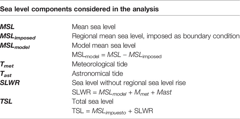
Table 2 lists the different components of the total sea level that are considered in the analysis. Total Sea Level (TSL) is arguably the most important variable to be considered when analyzing changes in sea level climate form a coastal engineering and coastal management viewpoint. However, to better understand these changes, their origin and their interactions, other variables are analyzed as well, namely: sea level without regional sea level rise (SLWR), model mean sea level (MSL_model), meteorological residuals (surge or meteorological tides; T_met) and tides (or astronomical tides; T_ast).

TABLE 2

Table 2 Sea level components considered in the analysis.

MSL_imposed is the imposed regional sea level rise and in consequence is uniform in the entire domain and does not depend on atmospheric forcing. On the other hand, MSL_model does depend on atmospheric forcing, but it has a spatial scale similar to that of the analysis region, being approximately uniform throughout the local domain. Both MSL_imposed and MSL_model are removed from the results to better analyze the other components of the sea level signal.

Changes in Tmet and T_ast are analyzed separately because they have different origin. While T_met depends on the atmospheric forcing, T_ast does not depend on the atmospheric forcing but can be affected by the nonlinear interactions with T_met and by the change in the MSL.

To obtain T_met at each point, first MSL_model is subtracted from the SLWR in order to avoid the influence of sea level components of spatial and temporal scales greater than that of the meteorological events (synoptic scale), and then the Doodson filter (Pugh, 1987) is applied to filter out astronomical tides from the signal. To obtain T_ast, an harmonic analysis is carried out using T-Tide toolbox (Pawlowicz et al., 2002), and only the amplitudes of the M2 and O1 components is analyzed, as these are the two most relevant components along the Uruguayan coast (Fossati et al., 2013).

For each variable the projected changes are evaluated by looking at changes in its mean value and in the 1% and 99% quantiles (the latter two representatives of extreme low and high conditions). Changes are evaluated considering results from each GCM separately and also by looking at the ensemble of the results.

2.5 Significance of the Projected Changes

The significance of the changes is analyzed only for the SLWR and its components. To analyze the significance of the changes projected by each GCM, the Student-t test was applied to the series of annual values of the three analyzed statistics (i.e. series of annual mean and of 1% and 99% quantiles; see e.g. Casas-Prat et al., 2017 and Hemer et al., 2013). Null hypothesis in this test is that the distribution of the annual statistics is the same in the historical period and in the future periods.

On the other hand, for the analysis of the ensemble of the results, the significance of the change is determined following a methodology similar to that used in Wandres et al. (2017) and Camus et al. (2017). For each model, the difference between the statistic estimated from projections and the one estimated in the historical period is calculated. Then, if the mean of the differences is greater than the standard deviation, and if at least 6 of the 7 models project the same direction of the change (increase or decrease), then the change in is said to be significant (i.e. when working with the ensemble of the results, a change is considered significant if both conditions are met).

3 Data

3.1 Measured Sea Level Series

Sea level data measured at six stations located in the study area are used for the calibration and validation of the local model. Of these, five stations are located along the Uruguayan coast and one in the inner part of the Río de la Plata estuary (Figure 1). Only years with less than 50% missing data are used in this study, considering the time period 1985-2005. Figure 4 shows the data availability at each station.

FIGURE 4

Figure 4 Measured data available in each station (only years with less than 50% missing data are considered).

3.2 Reanalysis CFSR

The calibration and validation of the hydrodynamic model is carried out by forcing it with hourly wind and SLP fields from the atmospheric reanalysis of the National Centers for Environmental Prediction NCEP-CFSR of USA (Saha et al., 2010). Wind data have a spatial resolution of 0.205°x0.204°, and SLP data have a spatial resolution of 0.312°x0.312° ¹. Here, only the data covering the historical period (1985-2005) is used.

3.3 Global Climate Models (GCMs)

To obtain sea level projections, the 2D hydrodynamic models are forced with wind and SLP fields of the seven GCM from the CMIP5 listed in Table 3. The selection of these models is made on the basis that these were the only models (at the moment of downloading, january 2019) having the required variables with temporal resolution of three-hours or higher. In all cases only r1i1p1 runs were used, and all data was downloaded through the Earth System Grid Federation².

TABLE 3

Table 3 CMIP5 models used in this study: name, institution, country and spatial resolution.

3.4 Mean Sea Level Rise

Regional sea level rise projections from IPCC AR5 (Church et al., 2013; IPCC, 2013) are used for climate scenarios RCP 4.5 and RCP 8.5 (data available from the Hamburg University³). Regional mean sea level rise data, relative to the baseline period 1986-2005, is available in a global domain with a 1°x1° resolution. In this work, the increase in mean sea level (we considered mean values of increase from the data set) is considered as uniform in space and is added to the boundary condition of the hydrodynamic model. This uniform regional mean sea level rise value is estimated as the spatial mean of the regional mean sea level rise within the computational domain of the hydrodynamic model, which includes the Río de la Plata and part of the Atlantic Ocean [lat (-54.2, -22) lon (-70, -45.5); see Figure 2].

Table 4 summarizes the estimated values of the regional sea level rise for four time-horizons and the mean rise for 2081-2100 period, for the two scenarios analyzed. It is noted that these values are in agreement with the values obtained when considering the regional sea level rise at the nodes closest to the Uruguayan coast (i.e. average regional sea level rise within the computational domain is in agreement with sea level rise projected for the Uruguayan coast and the Rio de la Plata estuary).

TABLE 4

Table 4 Mean sea level change used in this work for RCP 4.5 y RCP 8.5 scenarios.

4 Results

4.1 Local Model Calibration and Validation

The calibration of the local model results in choosing the Flather (1976) formulation for the wind shear stress and a non-uniform Manning number for the domain (0.007 in the inner zone of the estuary and 0.15 in outer and middle zones). Regarding validation, Figures 5, 6 show the scatter plots and the quantile-quantile plots for each station for total sea level (TSL) and meteorological residuals (or surge, T_met; see Projections of Change in Sea Level Climate), respectively. In addition, Table 5 lists RMSE and correlation coefficient for the different stations for both variables, along with the bias for the TSL.

FIGURE 5

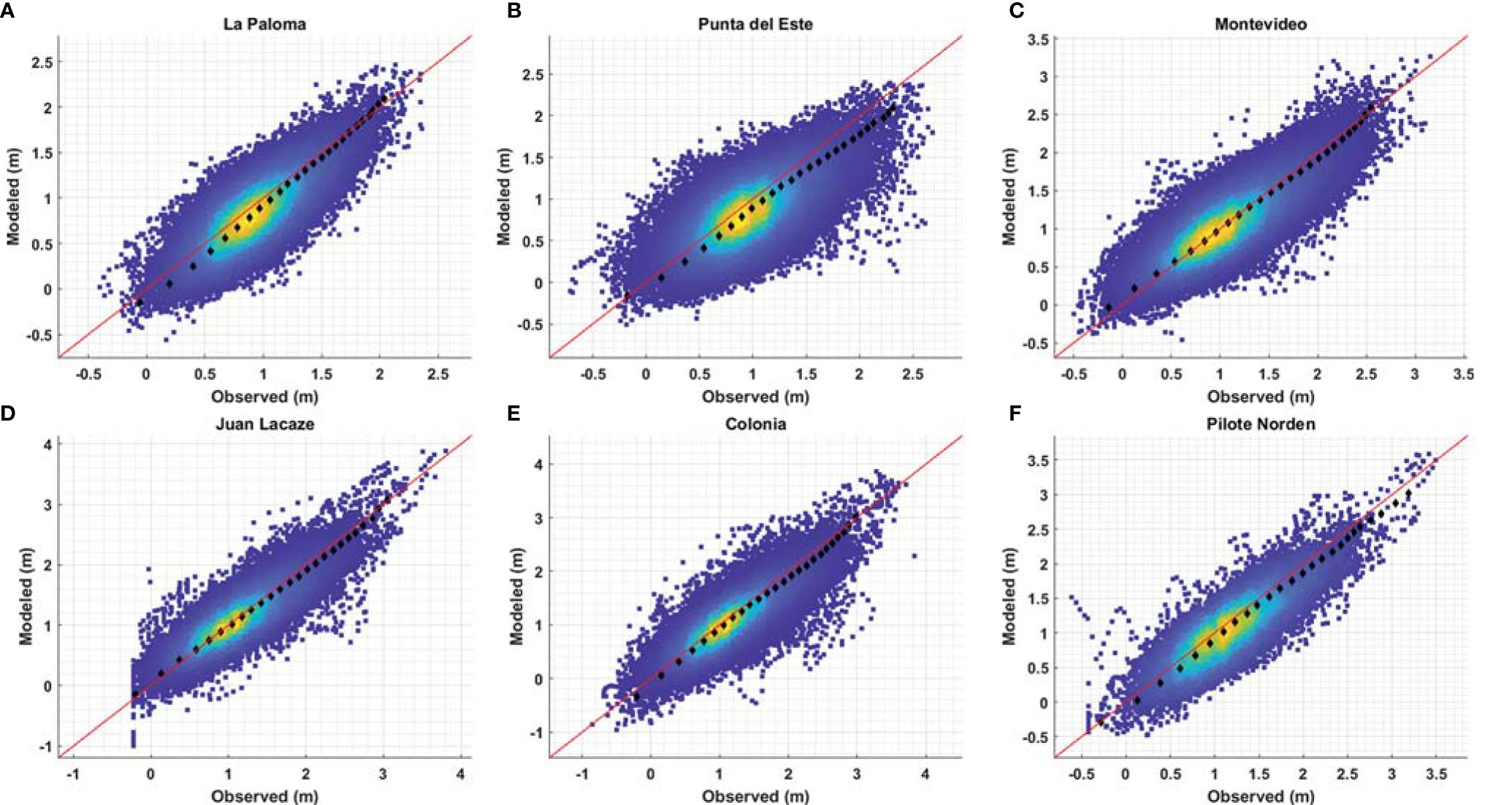
Figure 5 Scatter plot and qq-plot (black) from modeled total sea level (m) vs measured total sea level (m) in: (A) La Paloma, (B) Punta del Este, (C) Montevideo, (D) Juan Lacaze, (E) Colonia and (F) Pilote Norden. Only years with less than 50% hourly missing data considered. Read line represents 1-1 and colorscale represents data density (blue less data – yellow more data). 25 equispaced quantiles shown with Gumbel scale ranging from 0.001 to 0.999.

FIGURE 6

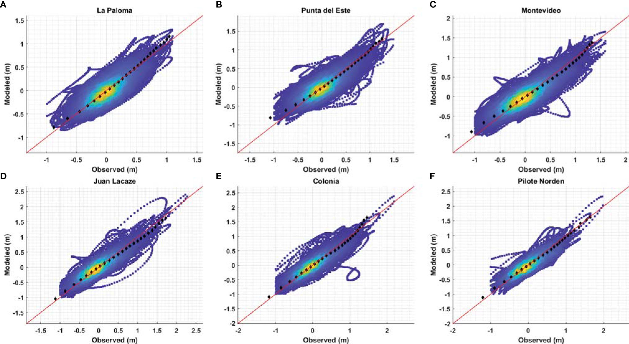
Figure 6 Scatter plot and qq-plot (black) from modeled meteorological tide (m) vs measured meteorological tide (m): (A) La Paloma, (B) Punta del Este, (C) Montevideo, (D) Juan Lacaze, (E) Colonia and (F) Pilote Norden. Only years with less than 50% hourly missing data considered. Read line represents 1-1 and colorscale represents data density (blue less data – yellow more data). 25 equispaced quantiles shown with Gumbel scale ranging from 0.001 to 0.999.

TABLE 5

Table 5 Stadistics obtained comparing modeled total sea level (BIAS, RMSE and r) and meteorological tide (RMSE and r) with measures in La Paloma, Punta del Este, Montevideo, Colonia, Juan Lacaze and Pilote Norden.

In Figure 5 it is observed that in all the stations the scatter points are aligned with the line 1-1 (indicated in red). In the case of Punta del Este, it is observed that the quantile-quantile plot shows a negative bias for all quantiles, in agreement with the high bias and RMSE and low correlation estimated for the TSL for this station (see Table 5). TSL at the rest of the stations present high correlation coefficients and RMSE values around 25 cm (Table 5). In Figure 6 it is noted that the scatter plots tend to be aligned with the identity line, although some points depart form the trend in some stations; in all cases the quantile-quantile plots are clearly aligned with the identity line. These is consistent with the large correlation coefficients listed for M_met in Table 5, although in this case the lowest correlations are obtained Punta del Este and La Paloma stations. Regarding astronomical tide, the model overestimates the amplitudes, reaching around 0.07 m and 0.04 m global RMSE values for M2 and O1 constituents respectively (considering only the coastal stations from Figure 1). Differences between measured and modeled amplitude and phase for each station are shown in Table S1. Nevertheless the model represents correctly the regional trend of the tide.

In general terms, the model correctly represents both the total sea levels and the meteorological component along the entire coast. These validated results are considered as the reference results from now on.

4.2 GCMs Historical Period

Figure 7 shows the quantile-quantile plots comparing TSL series obtained with the GCM with the reference series obtained with the CFSR at the 6 coastal stations presented in Figure 1, for the historical period. For the sake of readability, from now on when referring to results of a GCM, reference is made to the results obtained with the hydrodynamic model forced with that particular GCM. It is observed that the results get worse for the stations located at the inner part of the estuary (Colonia, Juan Lacaze and Pilote Norden).

FIGURE 7

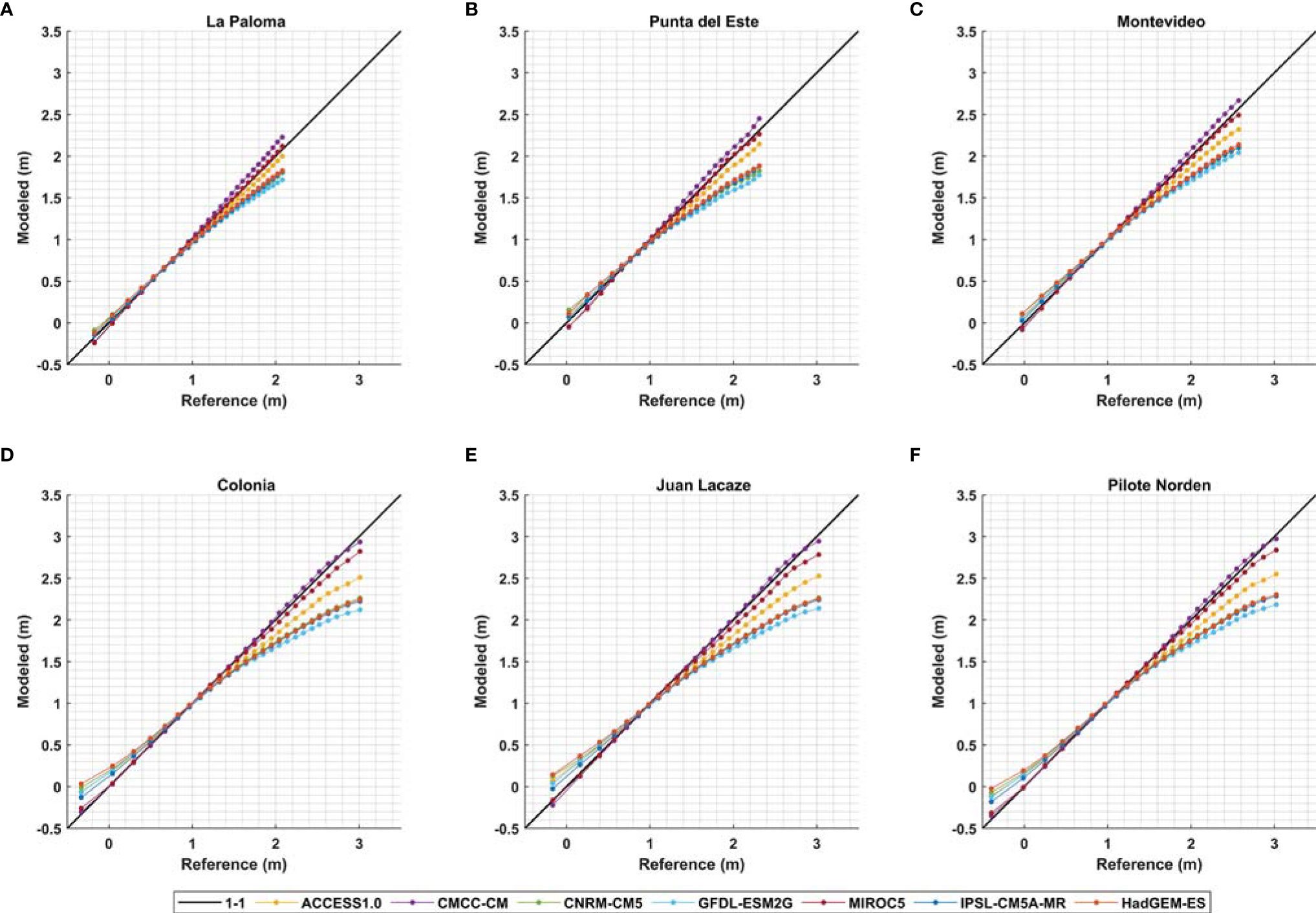
Figure 7 QQ-plots of data obtained from the local model forced with each GCM (Modeled) vs reference data (Reference) for the historical period (1986-2005): (A) La Paloma, (B) Punta del Este, (C) Montevideo, (D) Juan Lacaze, (E) Colonia and (F) Pilote Norden. 25 equispaced quantiles shown with Gumbel scale ranging from 0.001 to 0.999.

For the stations located at the outer part of the estuary and at the oceanic coast, a good performance is observed for all the GCM for low and middle quantiles; however, most of the GCM underestimate the high quantiles, with underestimations of up to 40 cm in La Paloma and 60 cm in Montevideo for the GFDL-ESM2G model. Exceptions are results from the MIROC5 and CMCC-CM models, for which the highest quantiles are well represented and tend to improve from La Paloma to Montevideo.

On the other hand, for stations at the inner part of the estuary, good results are observed for the MIROC5 and CMCC-CM models in the entire range of quantiles, while the rest of the models overestimate (underestimate) low (high) quantiles: lowest quantiles are overestimated by up to 30 cm, while highest quantiles are underestimated by up to 90 cm.

4.3 Projections

4.3.1 Changes in TSL

Figure 8 shows changes in the mean (left panels), 1% quantile (center panels) and 99% quantile (right panels) of the TSL, for both the short term (2027-2045) and long term (2082-2100) projections, and for both RCP scenarios. For the mean, a constant change is projected along the coast, while for the 1% and 99% quantiles it is observed that the projections of change vary along the coast.

FIGURE 8

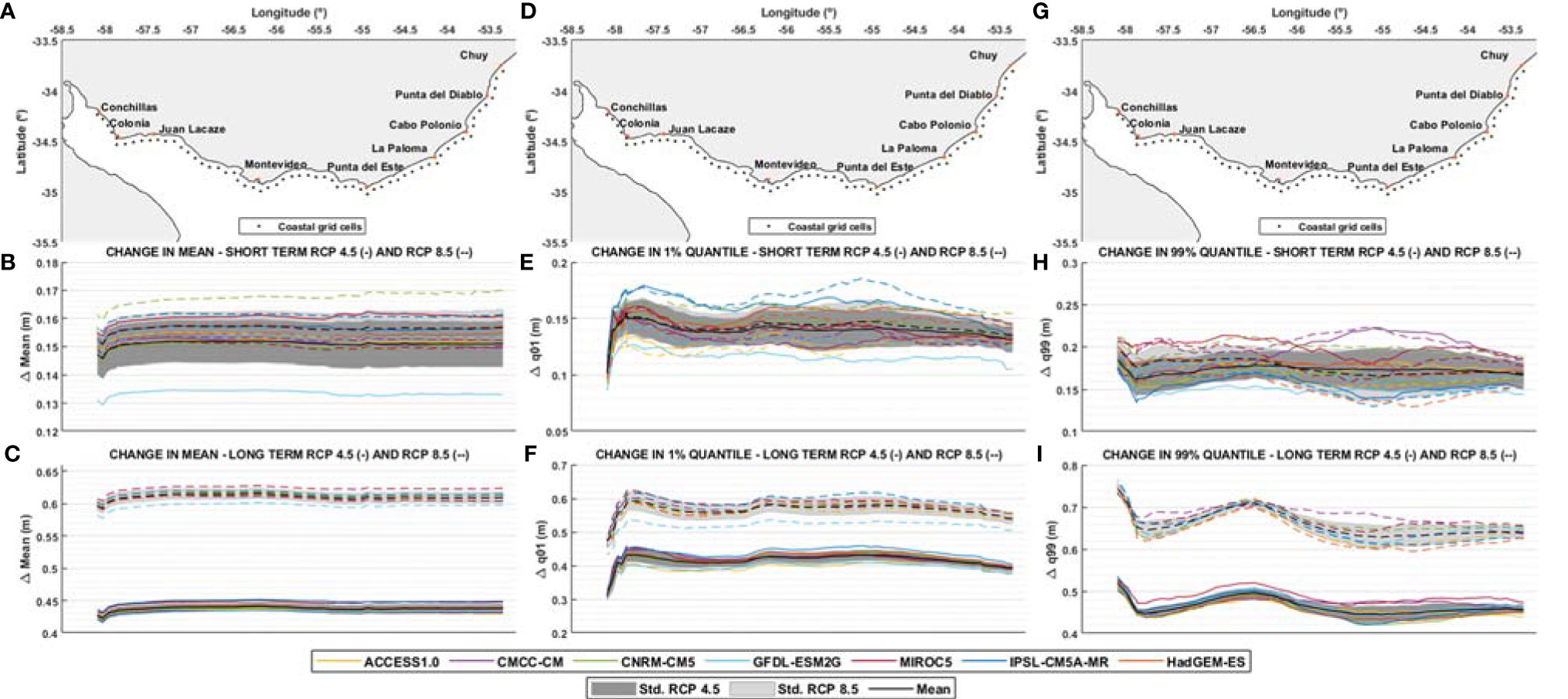
Figure 8 Change in mean (A–C), change in 1% quantile (D–F) and change in 99% quantile (G–I) of TSL obtained from local model forced with each GCM and ensemble (black), along the coast for short (2026-2045) and long term (2082-2100) and for RCP 4.5 (continuous lines) and RCP 8.5 (dotted lines). E.g.: change in 99% quantile for the short term is calculated as the difference between 2045-2026 99% quantile and 1985-2005 99% quantile. (A, D, G): coastal grid cells. (B, E, H): change for short term. (C, F, I): change for long term.

For the 1% quantile, a pattern of spatial variability is observed with a maximum around Colonia and a minimum between Juan Lacaze and Montevideo. In the short term, the range of projected changes is similar for both RCP scenarios. In the long term, the same spatial pattern is observed as in the short term, but with different ranges of variation for the different RCP (associated with differences in the mean sea level rise), and with larger differences between maximums and minimums.

On the other hand, changes in the short term of the 99% quantile shows a very similar range for the two scenarios and a relatively uniform pattern all along the coast. Whereas in the long term a marked spatial distribution is observed, with maximum values in the inner area of the estuary and a relative maximum around Montevideo, with similar behavior observed for both scenarios, although with different ranges of values.

From Figure 8 it is clear that the mean sea level rise dominates the projected changes in the TSL, therefore it is relevant to analyze changes in the SLWR and its components to better quantify and understand other sources of changes and their interactions.

4.3.2 Changes in the SLWR

Figure 9 shows the projected changes in the mean and in the 1% and 99% quantiles of the SLWR, for the long and short term and for both RCP scenarios, as well as the significance of the changes. It should be noted that the Student-t test, applied to each member of the ensemble, rejected the null hypothesis (i.e. changes are statistically significant) for all the nodes and for all the models and scenarios analyzed (for SLWR and for the variables T_met and T_ast analyzed next); therefore in Figure 9 and in those that follow, only the result of the significance of the changes in the ensembles is included.

FIGURE 9

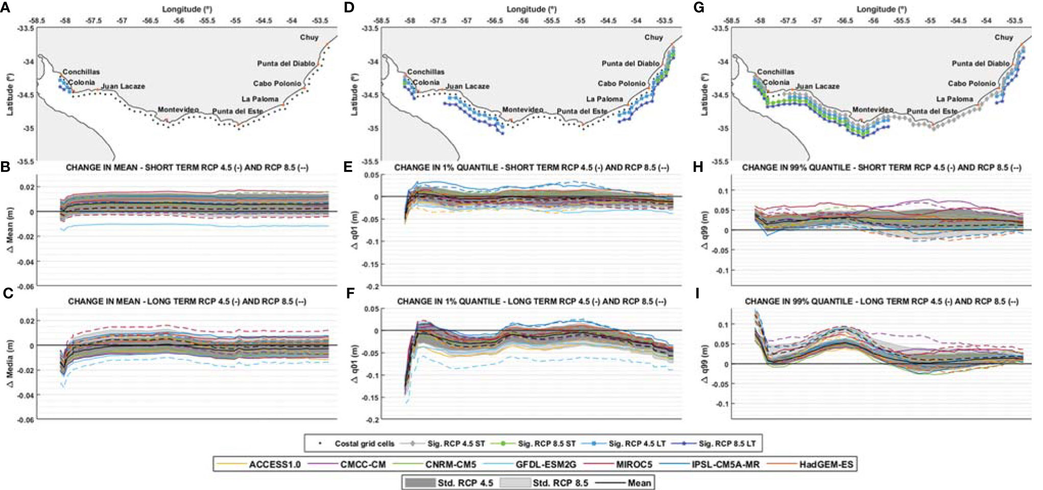
Figure 9 Change in mean (A–C), change in 1% quantile (D–F) and change in 99% quantile (G–I) of SLWR obtained from local model forced with each GCM and ensemble (black), along the coast for short (2026-2045) and long term (2082-2100) and for RCP 4.5 (continuous lines) and RCP 8.5 (dotted lines). E.g.: change in 99% quantile for the short term is calculated as the difference between 2045-2026 99% quantile and 1986-2005 99% quantile. (A, D, G): coastal grid cells and significance for the ensemble change for each scenario (the symbol indicates statistical significance of the ensemble change). (B, E, H): change for short term. (C, F, I): change for long term.

The change in the mean of the SLWR assembly is practically null and not significant along the entire coast, except for the innermost nodes in the long term, which indicates that the change in the mean of the TSL comes almost entirely from the increase in the mean sea level. On the other hand, the change in the 1% and 99% quantiles shows the same spatial patterns observed in the TSL.

The 1% quantile of the SLWR shows values very close to 0 in the short term along the entire coast for every scenario, although some significant negative changes are observed in the ensemble (less than 5 cm) for the RCP 8.5 scenario. In the long term, the spatial pattern of the changes is clearer, and the changes in the ensemble are significant in the inner zone of the estuary, between Juan Lacaze and Montevideo, as well as on the oceanic coast, from La Paloma to the East, for both scenarios. These changes show a minimum in the inner zone of the estuary, a relative minimum between Juan Lacaze and Montevideo, as well as a decrease from Punta del Este towards the east. It is noted that in the long term all the models show the same spatial pattern.

The 99% quantile of the SLWR shows significant changes in most of the coast for both future horizons and both scenarios. In the short term, the change is practically uniform along the coast for both scenarios, and the ensemble shows positive changes of less than 5 cm. In the long term, the same spatial pattern as for the change in TSL is observed, although in this case the maximums in the RCP8.5 scenario are more pronounced, which could be associated to either changes in the atmospheric patterns or to non-linear effects produced by the depth increase due to the mean sea level rise.

4.3.3 Change in the Meteorological Residuals (T_met)

Figure 10 shows the changes in the 1% and 99% quantiles of the T_met (by its definition, the mean value of T_met is always zero). The objective of analyzing this variable is to focus attention on the changes in sea level produced by changes in the atmospheric patterns in the region.

FIGURE 10

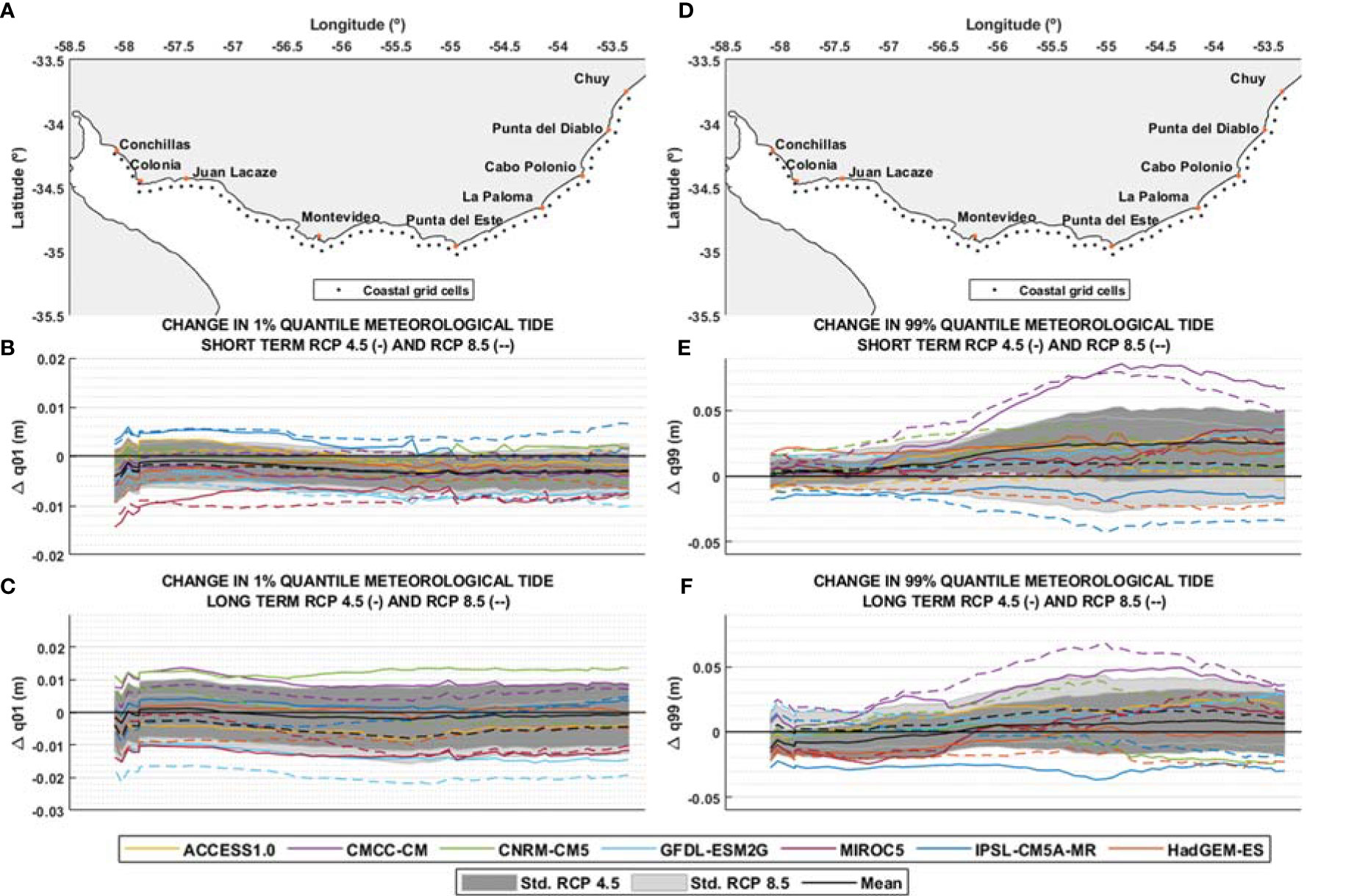
Figure 10 Change in 1% quantile (A–C) and change in 99% quantile (D–F) of T_met obtained from local model forced with each GCM and ensemble (black), along the coast for short (2026-2045) and long term (2082-2100) and for RCP 4.5 (continuous lines) and RCP 8.5 (dotted lines). E.g.: change in 99% quantile for the short term is calculated as the difference between 2045-2026 99% quantile and 1986-2005 99% quantile. (A, D): coastal grid cells. (B, E): change for short term. (C, F): change for long term.

It is observed that the projected change for the 1% quantile is small along the entire coast for all models and RCP scenarios, barely exceeding one centimeter in the short term and two centimeters in the long term. The maximum change in the 1% quantile occurs for the GFDL-ESM2G model in the long term and for the RCP 8.5 scenario, with a decrease of only 2 cm. It is noted that changes in the ensemble are not significant in all cases.

In general terms, the changes in the 99% quantile are small, although there is a slight trend towards positive changes towards the east, reaching values that exceed 5 cm in the short and long term for some of the models. In the inner area of the estuary, changes are negligible for all models. The model that shows the greatest changes is the CMCC-CM in all cases. The ensemble shows a clear trend to larger positive changes towards the east, with values not exceeding 2 cm in any case. As in the previous case, changes in the ensemble are not significant, mainly due to the great dispersion of the results.

4.3.4 Changes in the Astronomical Components (T_ast)

Figure 11 shows the projected changes in the amplitude of the tidal components M2 (right panel) and O1 (left panel), including the amplitude of both components for the historical period.

FIGURE 11

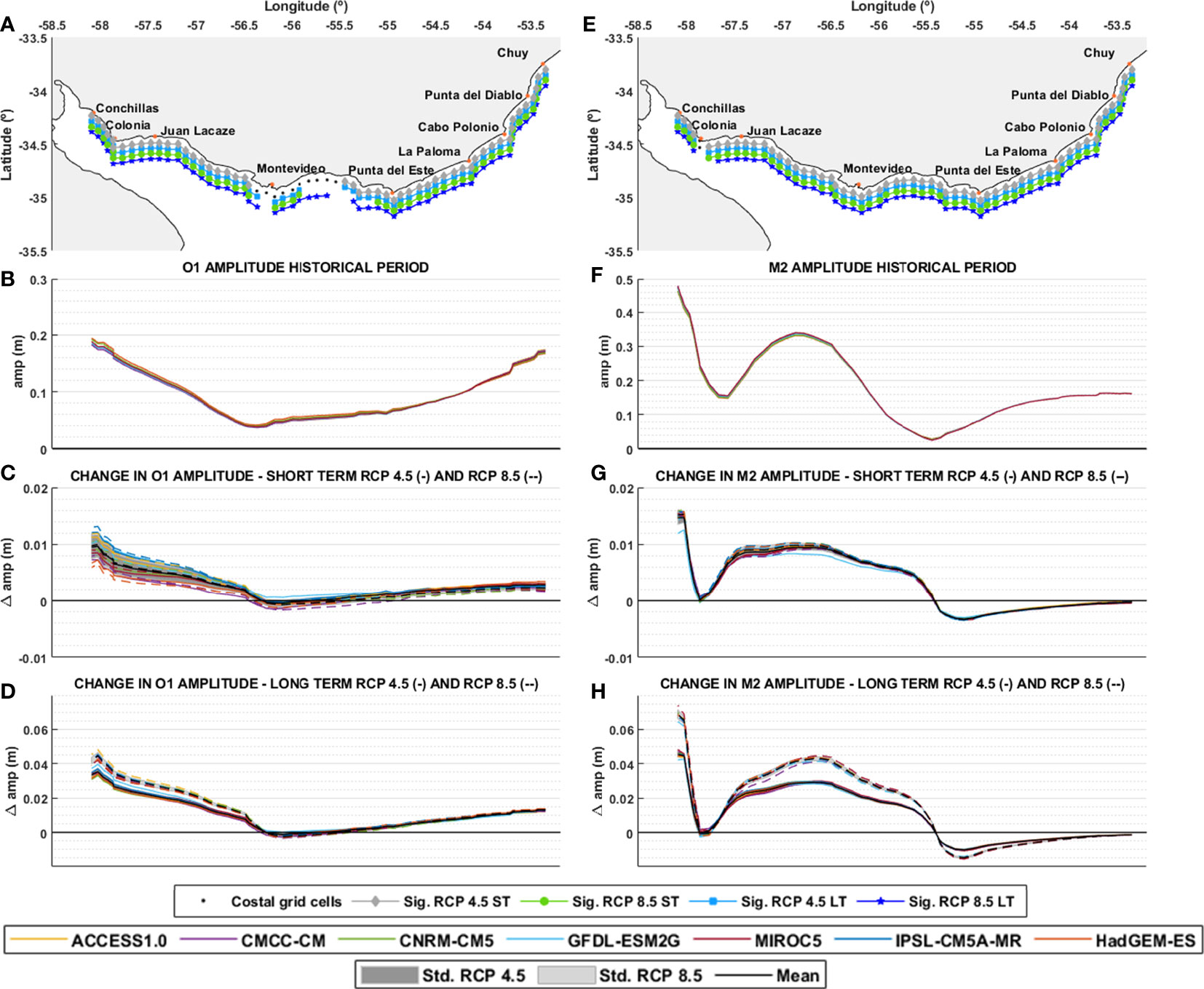
Figure 11 Change in O1 component amplitude (A–D) and change in M2 component amplitude (B–H) obtained from local model forced with each GCM and ensemble (black), along the coast for short (2026-2045) and long term (2082-2100) and for RCP 4.5 (continuous lines) and RCP 8.5 (dotted lines). E.g.: change in M2 component for the short term is calculated as the difference between 2045-2026 M2 amplitude and 1986-2005 M2 amplitude. (A, E) coastal grid cells coastal grid cells and significance for the ensemble change for each scenario (the symbol indicates statistical significance of the ensemble change), (B, F): component amplitude, (C, G): change for short term, (D, H): change for long term.

In the case of the M2 amplitude, it is seen that the spatial pattern of the changes along the coast is repeated in the short and long term, showing mostly positive changes for the amplitude of this component along almost the entire coast, with increases of about 1 cm in the short term and between 2 cm and 5 cm in the long term. It is noted that both the amplitude calculated for the historical period and the projected change have the same pattern, with relative maxima and minima almost coinciding in space. There is a relative minimum between Colonia and Juan Lacaze, with zero change in both the short and long term; then, there is another minimum in the amplitude between Montevideo and Punta del Este, also associated with zero change. In turn, near Punta del Este there is a significant negative change in both the short and long term. On the other hand, the largest projected changes occur for the largest amplitudes, in the inner zone of the estuary, where the maximum change in the short term reaches 1.5 cm and in the long term exceeds 4 cm for RCP 4.5 and 6 cm for RCP 8.5. Between Juan Lacaze and Montevideo there is a relative maximum in the amplitude of the M2 component that exceeds 30 cm; the changes for both time horizons also present a relative maximum in this zone, with short-term changes barely reaching one centimeter, and long-term changes exceeding 2 cm for RCP 4.5 and 4 cm for RCP 8.5. It should be noted that within each scenario and time horizon the dispersion of the results of the different models is small, resulting in all projected changes being significant for practically the entire coast. In addition, in the short term there is almost no difference in the projected changes for the different scenarios, while in the long term there are some differences between the scenarios, particularly in the magnitude of the projected changes.

The O1 component shows a similar behavior to that observed for the M2 component: the spatial pattern of the projected changes is similar to that of the amplitudes, with greater changes projected in the zones of higher amplitudes. Short-term changes show greater dispersion between models (with respect to that observed in M2), although they do not exceed one centimeter in any case. In the long term, there is a slight difference between scenarios, and the maximum change does not reach 4 cm for the RCP 4.5 scenario and barely exceeds 4 cm for the RCP 8.5 scenario, where the amplitude of the component is approximately 20 cm. As for the M2 component, the changes in the ensemble are significant along the coast.

5 Discussion

The results obtained by modeling the historical period, forcing the hydrodynamic models with the GCMs, show that a better representation of the sea level climate is achieved at the stations located in the outer estuary zone and in the oceanic coast. In particular, most GCMs underestimate the higher quantiles at all stations (except CMCC-CM at La Paloma, Punta del Este and Montevideo, and MIROC 5 at La Paloma), while the lower quantiles are well represented at the outer stations and overestimated at the inner stations. The models that best represent current sea level climate in the region are MIROC5 and CMCC-CM, which have a spatial resolution of 1.4°x1.4° (the lowest resolution among the 7 GCMs used) and 0.75°x0.75° (the highest resolution), respectively; thus, there seems to be no dependence between the resolution of the GCMs and their performance in modeling sea level climate. In any case, none of the models present results clearly at odds with the reference climatology, therefore it is reasonable to retain all of them when analyzing projections of change in order to have the widest possible range of results.

When analyzing the changes in TSL for all scenarios and future periods, it is observed that the change in the mean is uniform along the coast, dominated mainly by the increase in regional mean sea level. When analyzing the changes in the 1% and 99% quantiles of the SLWR, the influence of other components is observed, with a spatial pattern of changes that is not always uniform along the coast, which also emerge when analyzing the 1% and 99% quantiles of the TSL. The analysis of SLWR allows focusing attention on the changes induced in the tidal and surge wave dynamics resulting from the increase in the water depths due to the regional mean sea level rise. While the distribution of the 1% SLWR quantile does not yield additional information to that already observed in the distribution of the 1% TSL quantile (the SLWR shows almost overlapping changes for both scenarios, both in the short and long term), the analysis of the 99% SLWR quantile shows that in the long term for the RCP 8.5 scenario the change intensifies, obtaining differences of more than 5 cm between the maximum changes of the ensemble for each RCP scenario. It is possible to relate the latter to the interaction between tidal wave propagation and mean sea level rise, as in the future the difference between the mean sea level rise for both scenarios increase (see Table 4).

Regarding the meteorological residuals, both the 1% and 99% quantiles show changes close to 0 and not significant along the coast, for both the short and the long term. This indicates that the changes observed in the TSL are not associated with changes in the atmospheric circulation patterns. There are no previous studies of this type for our region, neither at global nor regional scales, but it is interesting to note that Vousdoukas et al., 2016) reach the opposite conclusion for the European coasts: these authors perform a dynamic downscaling of sea levels, forced with surface winds and SLP from 8 GCMs (without considering astronomical tides), finding that the increase in extreme levels associated with meteorological events along the European coast range from 15% to 40% in certain regions.

On the other hand, the changes in the amplitude of the M2 and O1 astronomical components along the coast were shown to be very similar between models. The general trend is to have large changes in areas of large tidal amplitude, and larger ratio between change and current amplitude for the O1 component than for the M2 component, with the former showing changes that reaches 4 cm for a current amplitude of 20 cm. It is also noted that the change in the astronomical components is not influenced by the atmospheric, as the 7 GCMs projected quite similar changes forcing (i.e. there are no strong tide-surge interaction affecting the changes), implying that changes in the astronomical tide amplitudes are due to the imposed regional mean sea level rise and the resulting increase in water depths.

From the previous analysis, it is clear that the main contribution to the change in the TSL is the regional mean sea level rise. Then, the analysis of the signals obtained by subtracting this contribution (SLWR and its components), shows that the change in the astronomical tide resulting from the increase in the regional mean sea level is especially important, and that it is from this interaction that arises the spatial patterns observed in the 1% and 99% quantiles (mainly in the latter). Moreover, since the change in MSL_model is constant along the coast, it is understood that it does not contribute significantly to the observed spatial patterns. On the other hand, the changes in the 99% quantile of the meteorological residual does not present the spatial pattern observed in TSL and SLWR, but shows minimum values along the coast towards the inner zone of the estuary and grows outwards. In contrast, the change along the coast in the tidal components does present a spatial pattern that agrees with that observed in the SLWR, especially in the inner zone of the estuary, where the change for the M2 and O1 component are maximum. In particular, the M2 component presents a relative maximum that encompasses the zone of maximum change around Montevideo observed in the TSL and SLWR, which leads to think that it may also be contributing significantly to these, although for the M2 component the zone of change extends almost to Punta del Este, unlike for the SLWR. All the above agrees with the fact that changes in the 99% quantile intensify in the long term with the more severe scenario, given that the difference in regional mean sea level rise between scenarios increases in the long term. It is noted that this result is consistent with that of Pickering et al. (2012); Pelling et al. (2013) and Idier et al. (2017) for the European shelf, where they analyzed the effect of the mean sea level rise on the astronomical tide, confirming the importance of the interaction between the mean sea level change and the tides: Idier et al. (2017) concludes that changes of up to +/-15% are reached in the amplitudes of the most important tidal components in the region, such as M2, S2, N2, among others; Pickering et al. (2017) investigated the effect of mean sea level rise on the tides globally, concluding that significant changes occur in the M2 and S2 constituents in most shelf seas. Moreover, Haigh et al. (2020) does a comprehensive review of past and future non-astronomical changes in tides, concluding regional increases and decreases in tides are likely to occur in response to MSL rise, changes in coastal morphology and variations in ice sheets extension, affecting particularly shelf seas and coastal waters; Howard et al. (2019) provided a synthesis of results of projections of 21^st century change in extreme sea levels around the coast of the United Kingdom and reached similar conclusions as this work, finding projections dominated by the effects of the mean sea level rise and changes in tidal amplitudes induced by it, also noting that the tidal changes do not depend on the atmospheric forcing (i.e. on the GCM forcing model), being these highly uncertain, what makes changes in tidal amplitudes more robust.

There are certain limitations in this work that are worth highlighting. First, the number of GCMs available for analysis was relatively small, which is detrimental to the robustness of the projections; although criteria have been implemented to determine when a change is significant, having a small number of models increases the risk of not being able to differentiate between climate trends and the internal variability of the GCMs used. In any case, this problem may be overcome in future studies using the growing number of GCM results made available by CMIP for dynamic downscaling. A second limitation is related to the use of two-dimensional models, since they cannot capture variations in mean sea level due to changes in the baroclinic structure of the oceans; Hermans et al., 2020 have shown that this effect is significant in the case of the North Sea, so it should be included in future studies in order to analyzes its relevance in this region. Lastly, this work used sea level rise projections corresponding to AR5 (IPCC, 2013), which were improved in the SROCC (IPCC, 2019) and for AR6 (Fox-Kemper et al., 2021). However, comparison of CMIP5 and CMIP6 shows that there are no qualitative differences in sea level rise projections, and that quantitative differences are limited to a few centimeters (see e.g. Hermans et al., 2020, Lyu et al., 2020), so it seems that updated regional sea level rise values would lead to similar results in our work.

6 Conclusions

From the analysis of the changes projected for the different components of the total sea level along the Uruguayan coast, it is concluded that the main contribution to the projected changes is the regional mean sea level rise, followed in importance by the effect that the increase in the water depth has on the amplitude of the tidal components. Moreover, it is concluded that changes in the meteorological residuals, associated with potential changes in the atmospheric circulation patterns, are negligible in the study area. This in turn reinforces the need to resort to dynamic downscaling for studies of these characteristics, since this approach allows to resolve the interactions that may arise between tides, surges and the mean sea level rise, something that cannot addressed with an approach based solely on statistical downscaling.

Regarding the magnitude of the projected changes for the Uruguayan coast, there are two regions along the coast that deserve special attention, as there is where the greatest increases in the 99% quantile of the TSL is projected: from Colonia towards the inner part of the estuary and the coastal zone around Montevideo. In the long term (2082-2100) the ensemble shows increases of up to 52 cm in Colonia and 50 cm around Montevideo for RCP 4.5, with around 46 cm explained by the 2081-2100 mean sea level rise. For RCP 8.5, the ensemble shows increases up to 74 cm in Colonia towards the inner part of the estuary and 71 cm around Montevideo, where 64 cm comes from 2081-2100 mean sea level rise.

Data Availability Statement

The raw data supporting the conclusions of this article will be made available upon reasonable request. Requests to access the datasets should be directed to Michelle Jackson, bWphY2tzb25AZmluZy5lZHUudXk=.

Author Contributions

MJ, MF, and SS designed the research and wrote the paper. MJ performed the research, process the data and analyzed the results. MF and SS advised all the research and analysis. All authors contributed to the article and approved the submitted version.

Conflict of Interest

The authors declare that the research was conducted in the absence of any commercial or financial relationships that could be construed as a potential conflict of interest.

Publisher’s Note

All claims expressed in this article are solely those of the authors and do not necessarily represent those of their affiliated organizations, or those of the publisher, the editors and the reviewers. Any product that may be evaluated in this article, or claim that may be made by its manufacturer, is not guaranteed or endorsed by the publisher.

Acknowledgments

We acknowledge the World Climate Research Programme’s Working Group on Coupled Modelling, which is responsible for CMIP, and we thank the climate modeling groups (listed in Table 3 of this paper) for producing and making available their model output. For CMIP the U.S. Department of Energy’s Program for Climate Model Diagnosis and Intercomparison provides coordinating support and led development of software infrastructure in partnership with the Global Organization for Earth System Science Portals.

Supplementary Material

The Supplementary Material for this article can be found online at: https://www.frontiersin.org/articles/10.3389/fmars.2022.846396/full#supplementary-material

Footnotes

1. ^ https://rda.ucar.edu/.
2. ^ https://esgf-node.llnl.gov.
3. ^ https://icdc.cen.uni-hamburg.de/thredds/catalog/ftpthredds/ar5_sea_level_rise/catalog.html.

References

Briere C., Abadie S., Bretel P., Lang P. (2007). Assessment of TELEMAC Systemperformances, a Hydrodynamic Case Study of Anglet, France. Coast Eng. 54, 345–356. doi: 10.1016/j.coastaleng.2006.10.006

CrossRef Full Text | Google Scholar

Camus P., Losada I. J., Izaguirre C., Espejo A., Menéndez M., Pérez J. (2017). Statistical Wave Climate Projections for Coastal Impact Assessments. Earth’s Future 5, 918–933. doi: 10.1002/2017EF000609

CrossRef Full Text | Google Scholar

Camus P., Menéndez M., Méndez F. J., Izaguirre C., Espejo A., Cánovas V., et al. (2014). A Weather-Type Statistical Downscaling Framework for Ocean Wave Climate. J. Geophys. Res.: Oceans 119, 7389–7405. doi: 10.1002/2014JC010141

CrossRef Full Text | Google Scholar

Carson M., Kohl A., Stammer D., Slangen A. B. A., Katsman C. A., Van de Wal R. S. A., et al. (2016). Coastal Sea Level Changes, Observed and Projected During the 20^th and 21^st Century. Clim. Chang. 134, 269–218. doi: 10.1007/s10584-015-1520-1

CrossRef Full Text | Google Scholar

Casas-Prat M., Wang X. L., Swart N. (2017). CMIP5-Based Global Wave Climate Projections Including the Arctic Ocean. Ocean Model. 123, 66–85. doi: 10.1016/j.ocemod.2017.12.003

CrossRef Full Text | Google Scholar

Church J., Clark P., Cazenave A., Gregory J., Jevrejeva S., Merrifield M., et al. (2013). “Sea Level Change, Pages 1137–1216. Climate Change 2013: The Physical Science Basis,” in Contribution of Working Group I to the Fifth Assessment Report of the Intergovernmental Panel on Climate Change, vol. 13. (Cambridge, UK and New York, NY, USA: Cambridge University Press), 1137–1216.

Google Scholar

Eyring V., Bony S., Meehl G. A., Senior C. A., Stevens B., Stouffer R. J., et al. (2016). Overview of the Coupled Model Intercomparision Project Phase 6 (CMIP6) Experimental Design and Organization. Geosci. Model Dev. 9, 1937–1958. doi: 10.5194/gmd-9-1937-2016

CrossRef Full Text | Google Scholar

Fernández M., Piedra-Cueva I. (2011). “Revisión De Un Modelo Regional De Marea Astronómica Implementado Sobre La Región Suroeste Del Océano Atlántico,” in Tesis De Maestría En Mecánica De Los Fluidos. (Montevideo, Uruguay: Universidad de la República).

Google Scholar

Flather R. (1976). Results From Surge Prediction Model of the North-West 15uantifi Continental Shelf for 15uant, 15uantifi and 15uantifi 1973. Report 24 (Wormley, UK: Institute of Oceanography (UK).

Google Scholar

Fossati M., Santoro P., Mosquera R., Martínez C., Ghiardo F., Ezzatti P., et al. (2013). Dinámica De Flujo, Del Campo Salino Y De Los Sedimentos Finos En El Río De La Plata. RIBAGUA-Revista Iberoam. del Agua 1, 48–63. doi: 10.1016/S2386-3781(15)30007-4

CrossRef Full Text | Google Scholar

Fox-Kemper B., Hewitt H. T., Xiao C., Aðalgeirsdóttir G., Drijfhout S. S., Edwards T. L., et al. (2021). “Ocean, Cryosphere and Sea Level Change,” in Climate Change 2021: The Physical Science Basis. Contribution of Working Group I to the Sixth Assessment Report of the Intergovernmental Panel on Climate Change. Eds. Masson-Delmotte V., Zhai P., Pirani A., Connors S. L., Péan C., Berger S., Caud N., Chen Y., Goldfarb L., Gomis M. I., Huang M., Leitzell K., Lonnoy E., Matthews J. B. R., Waterfield T., Yelekçi O., Yu R., Zhou B. (Cambridge University Press).

Google Scholar

Guillou N., Chapalain G. (2012). Modeling Penetration of Tide-Influenced Waves in Le Havre Harbor. J. Coast Res. 28, 945–955. doi: 10.2112/JCOASTRES-D-11-00192.1

CrossRef Full Text | Google Scholar

Haigh I. D., Pickering M. D., Green J. M., Arbic B. K., Arns A., Dangendorf S., et al. (2020). The Tides They are A-Changin’: A Comprehensive Review of Past and Future Nonastronomical Changes in Tides, Their Driving Mechanisms, and Future Implications. Rev. Geophys. 58 (1). doi: 10.1029/2018RG000636

CrossRef Full Text | Google Scholar

Hemer M. A., Katzfey J., Trenham C. (2013). Global Dynamical Projections of Surface Ocean Wave Climate for a Future High Greenhouse Gas Emission Scenario. Ocean Modell. 70, 221–245. doi: 10.1016/j.ocemod.2012.09.008

CrossRef Full Text | Google Scholar

Hemer M. A., Trenham C. E. (2015). Evaluation of a CMIP5 Derived Dynamical Global Wind Wave Climate Model Ensemble. Ocean Modell. 103, 190–203. doi: 10.1016/j.ocemod.2015.10.009

CrossRef Full Text | Google Scholar

Hermans T. H. J., Tinker J., Palmer M. D., Katsman C. A., Vermeersen B. L. A., Slangen A. B. A. (2020). Improving Sea-Level Projections on the Northwestern European Shelf Using Dynamical Downscaling. Climate Dyn. 54(3-4), 1987–2011. doi: 10.1007/s00382-019-05104-5

CrossRef Full Text | Google Scholar

Hervouet J. M. (2007). Hydrodynamics of Free Surface Flows: Modelling With the Finite Element Method (Chichester, UK: John Wiley & Sons Ltd).

Google Scholar

Howard T., Palmer M. D., Bricheno L. M. (2019). Contributions to 21st Century Projections of Extreme Sea-Level Change Around the Uk. Environ. Res. Commun. 1 (9), 095002. doi: 10.1088/2515-7620/ab42d7

CrossRef Full Text | Google Scholar

Huybrechts N., Villaret C. (2013). Large Scale Morphodynamic Modeling of the Gironde Estuary. Proc. Inst. Civ. Eng. Marit. Eng. 166 (2), 51–62. doi: 10.1680/maen.2012.18

CrossRef Full Text | Google Scholar

Huybrechts N., Villaret C., Lyard F. (2012). Optimized Predictive 2D Hydrodynamic Model of the Gironde Estuary (France). J. Waterw. Port Coast. Ocean Eng. 138 (4), 312–322. doi: 10.1061/(ASCE)WW.1943-5460.0000129

CrossRef Full Text | Google Scholar

Idier D., Paris F., Le Cozannet G., Boulahya F., Dumas F. (2017). Sea-Level Rise Impacts on the Tides of the European Shelf. Cont. Shelf Res. 137, 56–71. doi: 10.1016/j.csr.2017.01.007

CrossRef Full Text | Google Scholar

IPCC (2013). Climate Change 2013: The Physical Science Basis. Contribution of Working Group I to the Fifth 17uantifica Report of the Intergovernamental Panel on Climate Change (Cambridge, United Kingdom and New York, NY, USA: Cambridge University Press).

Google Scholar

IPCC (2019). Summary for Policymakers. Special Report on the Ocean and Cryosphere in a Changing Climate (Cambridge, United Kingdom and New York, NY, USA: Cambridge University Press).

Google Scholar

Jackson M., Fossati M., Solari S. (2021). Cuantificación De Los Efectos Del Cambio Climático Sobre El Régimen Medio Y Extremal Del Nivel De Mar En La Costa Uruguaya. Tesis De Maestría En Mecánica De Los Fluidos (In Spanish). (Montevideo, Uruguay: Universidad de la República).

Google Scholar

Jones J. E., Davies A. M. (2008). Storm Surge Computations for the West Coast of Britainusing a Finite Element Model (TELEMAC). Ocean Dyn 58, 337–363. doi: 10.1007/s10236-008-0140-y

CrossRef Full Text | Google Scholar

Luo J., Li M., Sun Z., O'Connor B. A. (2013). Numerical Modelling of Hydrodynamics and Sand Transport in the Tide-Dominated Coastal-to-Estuarine Region. Mar. Geol 342, 14–27. doi: 10.1016/j.margeo.2013.06.004

CrossRef Full Text | Google Scholar

Lyard F., Lefevre F., Letellier T., Francis O. (2006). Modelling the Global Ocean Tides: Modern Insights From FES2004. Ocean Dyn Vol. 56 pp, 394–415. doi: 10.1007/s10236-006-0086-x

CrossRef Full Text | Google Scholar

Lyu K., Zhang X., Church J. A. (2020). Regional Dynamic Sea Level Simulated in the CMIP5 and CMIP6 Models: Mean Biases, Future Projections, and Their Linkages. J. Climate 33 (15), 6377–6398. doi: 10.1175/JCLI-D-19-1029.1

CrossRef Full Text | Google Scholar

Martínez C., Silva J. P., Dufrechou E., Santoro P., Fossati M., Ezzati P., et al. (2015). “Towards a 3D Hydrodynamic Numerical Modeling System for Long Term Simulations of the Río De La Plata Dynamic,” in E-proceedings of the 36th IAHR World Congress, The Hague, the Netherlands.

Google Scholar

Mateus M., Neves R. (2013). Ocean Modelling for Coastal Management – Case Studies With MOHID (Lisbon, Portugal: IST Press).

Google Scholar

Meucci A., Young I. R., Hemer M., Kirezci E., Ranasinghe R. (2020). Projected 21st Century Changes in Extreme Wind-Wave Events. Sci. Adv. 6, 7295–7305. doi: 10.1126/sciadv.aaz7295

CrossRef Full Text | Google Scholar

Moss R. H., co-authors (2010). The Next Generation of Scenarios for Climate Change Research and Assessment. Nature 463, 747–756. doi: 10.1038/nature08823

PubMed Abstract | CrossRef Full Text | Google Scholar

Pawlowicz R., Beardsley B., Lentz S. (2002). Classical Tidal Harmonic Analysis Including Error Estimates in MATLAB Using T_TIDE. Comput. Geosci. 28, 929–937. doi: 10.1016/S0098-3004(02)00013-4

CrossRef Full Text | Google Scholar

Pelling H., Green M., Ward S. (2013). Modelling Tides and Sea-Level Rise: To Flood or Not to Flood. Ocean Modell. 63, 21–29. doi: 10.1016/j.ocemod.2012.12.004

CrossRef Full Text | Google Scholar

Perez J., Menendez M., Camus P., Mendez F. J., Losada I. J. (2015). Statistical Multi-Model Climate Projections of Surface Ocean Waves in Europe. Ocean Modell. 96, 161–170. doi: 10.1016/j.ocemod.2015.06.001

CrossRef Full Text | Google Scholar

Pickering M., Horsburgh K., Blundell J. R., Hirschi J., Nicholls R. J., Verlaan M., et al. (2017). The Impact of Future Sea-Level Rise on the Global Tides. Cont. Shelf Res. 142, 50–68. doi: 10.1016/j.csr.2017.02.004

CrossRef Full Text | Google Scholar

Pickering M., Wells N., Horsburgh K., Green M. (2012). The Impact of Future Sea-Level Rise on the European Shelf Tides. Cont. Shelf Res. 35, 1–15. doi: 10.1016/j.csr.2011.11.011

CrossRef Full Text | Google Scholar

Pugh D. T. (1987). Tides, Surges and Mean Sea Level (Swindon, UK: Natural Environment Research Council).

Google Scholar

Saha S., Moorthi S., Pan H.-L., Wu X., Wang J. (2010). The NCEP Climate Forecast System Reanalysis. Bull. Am. Meteorol Soc. 91 (8), 1015–1058. doi: 10.1175/2010BAMS3001.1

CrossRef Full Text | Google Scholar

Santoro P., Fossati M., Piedra-Cueva I. (2013). Study of the Meteorological Tide in the Río De La Plata. Cont. Shelf Res. 60, 51–63. doi: 10.1016/j.csr.2013.04.018

CrossRef Full Text | Google Scholar

Sathish Kumar S., Balaji R. (2015). Effect of Bottom Friction on Tidal Hydrodynamics Along Gulf of Khambhat, India. Estuarine Coastal Shelf Sci. 154, 129. doi: 10.1016/j.ecss.2015.01.012

CrossRef Full Text | Google Scholar

Slangen A. B. A., Carson M., Katskman C. A., van de Wal R. S. W., Kohl A., Vermeersen L. L. A., et al. (2014). Projecting Twenty-First Century Regional Sea-Level Changes. Clim. Chang. 124, 317–332. doi: 10.1007/s10584-014-1080-9

CrossRef Full Text | Google Scholar

Taylor K. E., Stouffer R. J., Meehl G. A. (2012). An Overview of CMIP5 and the Experiment Design. Bull. Am. Meteorol Soc. 93, 485–498. doi: 10.1175/BAMS-D-11-00094.1

CrossRef Full Text | Google Scholar

Vousdoukas M. I., Voukouvalas E., Annunziato A., Giardino A., Feyen L. (2016). Projections of Extreme Storm Surge Levels Along Europe. Climate Dyn. 47, 3171–3190. doi: 10.1007/s00382-016-3019-5

CrossRef Full Text | Google Scholar

Wandres M., Pattiaratchi C., Hemer M. A. (2017). Projected Changes of the Southwest Australian Wave Climate Under Two Atmospheric Greenhouse Gas Concentration Pathways. Ocean Modell. 117, 70–87. doi: 10.1016/j.ocemod.2017.08.002

CrossRef Full Text | Google Scholar

Wang X. L., Feng Y., Swail V. R. (2014). Changes in Global Ocean Wave Heights as Projected Using Multimodel CMIP5 Simulations. Geophys. Res. Lett. 41, 1026–1034. doi: 10.1002/2013GL058650

CrossRef Full Text | Google Scholar