Flow Structure in an Artificial Seagrass Meadow in Combined Wave-Current Conditions

Experiments were conducted in a laboratory flume using an artificial seagrass meadow, modeled after Zostera marina, to examine the impact of waves on the vertical structure of time-averaged current, Reynolds stress, and turbulent kinetic energy (TKE) under combined wave-current conditions. With the addition of smaller waves, defined by a ratio of wave velocity to current velocity U_w/U_c < 2.5, the time-averaged velocity peaked above the meadow, which was similar to pure current conditions. When U_w/U_c > 2.5, the presence of waves caused the time-averaged velocity to peak near the top of the meadow. For U_w/U_c > 1 the presence of waves reduced the magnitude of peak Reynolds stress. For all conditions considered, the wake production of turbulence dominated the shear production of turbulence in the meadow. However, the wave velocity was less efficient than the current velocity in generating TKE in the meadow because the movement of the blades forced by the oscillatory fluid motion reduced the relative velocity between the blades and the wave. A modified hybrid model for wake production of TKE in a flexible canopy under combined wave-current conditions was proposed to account for the relative contributions of waves and currents. Wake production of TKE was dominated by waves when U_w/U_c > 1 and dominated by currents when U_w/U_c < 1. The models and observations proposed in this study contribute to an enhanced understanding of the relative influences of waves and currents on seagrass meadow flow structure in realistic combined wave-current conditions.

Introduction

Meadows of submerged aquatic vegetation, such as seagrass, can damp wave energy (e.g., Knutson et al., 1982; Fonseca and Cahalan, 1992), reduce erosion, and improve water quality (e.g., Ginsburg and Lowenstam, 1958; Ward et al., 1984; Moore, 2004). The reduction of current velocity within the meadow enhances the creation of near-bed habitat relative to unvegetated regions (e.g., Fonseca et al., 1982; Homziak et al., 1982). These ecosystem services depend on the interactions between the meadow, waves, and current. For example, hydrodynamic intensity impacts seagrass nutrient uptake (e.g., Lei and Nepf, 2016; Gillis et al., 2017) and overall seagrass survival (Peralta et al., 2006; Fonseca et al., 2007). Furthermore, the initiation of sediment transport within vegetated regions has been linked to exceeding thresholds of vegetation-generated turbulence in pure current (Yang et al., 2016) and pure wave (Tinoco and Coco, 2018; Tang et al., 2019; Zhang and Nepf, 2019) conditions. This paper describes mean and turbulent flow within submerged aquatic vegetation under combined wave-current conditions, which can provide a deeper understanding of meadow hydrodynamics and enable a more accurate assessment of ecosystem services.

Under unidirectional flow, vegetation drag reduces velocity within the meadow and redirects some flow over the top of the meadow, creating a shear layer with an inflection point in the vertical profile of time-averaged velocity (Brunet et al., 1994; Raupach et al., 1996; Ghisalberti and Nepf, 2006). The shear layer at the top of the meadow, as well as the wakes of individual shoots and leaves, can convert mean kinetic energy into turbulent kinetic energy (e.g., Nepf, 1999; Nepf and Vivoni, 2000; Tanino and Nepf, 2008). In pure wave conditions, stem wake turbulence is generated in proportion to the wave velocity squared (Zhang et al., 2018; Tang et al., 2019; Zhang and Nepf, 2019), but shear layer turbulence is only generated for long waves for which the wave excursion significantly exceeds the drag length scale of the canopy (Ghisalberti and Schlosser, 2013).

Turbulence has been studied in pure current and pure wave conditions separately, but waves and currents can coexist in seagrass meadows (e.g., Koch et al., 2006). Multiple studies have considered turbulence in combined wave-current conditions in rigid and flexible meadows of model vegetation. Both Lou et al. (2018) and Chen et al. (2020) observed that the addition of waves increased turbulent kinetic energy (TKE) within dense arrays of rigid cylinders relative to pure currents. In a flexible meadow, the individual plants may deflect under currents and sway under waves, changing the structure of time-averaged and turbulent velocities. For example, in pure current conditions, oscillations in the meadow height (known as monami) decrease the sharpness of the drag interface at the top of the canopy and the magnitude of peak Reynolds stress, relative to stationary canopies (Ghisalberti and Nepf, 2006). The presence of waves can cause a mean pronation in the direction of wave propagation (e.g., Zhang et al., 2018). Paul and Gillis (2015) subjected a transplanted meadow of Zostera noltei to both pure current and combined wave-current conditions and observed no differences in time-averaged velocity, but observed a reduction in TKE in combined wave-current conditions relative to corresponding pure current conditions, which is opposite to the trend observed for rigid models (e.g., Lou et al., 2018; Chen et al., 2020). In a field study on a floodplain of the Yangtze River and for multiple species of flexible vegetation, Zhang et al. (2021) observed little impact of waves on the magnitude of TKE associated with the current, but observed that the presence of waves increased the shear layer penetration depth, δ_e, relative to that predicted for pure current (Nepf et al., 2007), and they attributed this to the waving of the flexible leaves.

The primary goal of this study was to observe the influence of wave amplitude on time-mean flow structure, Reynolds stress, and TKE in combined wave-current conditions within a flexible meadow, including an evaluation of TKE prediction in combined wave-current conditions. Understanding how the combination of waves and currents impacts flow structure and turbulence in a seagrass meadow can improve the description of seagrass meadow hydrodynamics and the ecosystem services those conditions facilitate.

Theoretical Background for Predicting Velocity and Turbulence in Meadow

Several studies have described unidirectional flow over a rigid submerged meadow using a two-layer model: an overflow layer, with depth- and time-averaged velocity U₂, and a canopy layer of height h, with depth- and time-averaged velocity U₁ (e.g., Huthoff et al., 2007; Cheng, 2011; Chen et al., 2013; see Figure 1). This was modified for a flexible meadow by Lei and Nepf (2021), who incorporated the impact of plant reconfiguration by using the deflected canopy height, h_d, and the effective blade length, l_e, defined in Luhar and Nepf (2011, 2013) as the length of rigid blade that provides the equivalent drag to a flexible blade of length l. Specifically, for a depth-averaged velocity U_c in total water depth D, the in-canopy velocity is

$\begin{array}{c}\hfill U_1=\frac{U_c}{1-\frac{h_d}{D}\mathrm{\varphi }+\sqrt{\frac{C_D{a}_v{l}_e}{2C\left(1-\mathrm{\varphi }\right)}{\left(\frac{D-h_d}{D}\right)}^3}}\hfill \end{array}(1)$

FIGURE 1

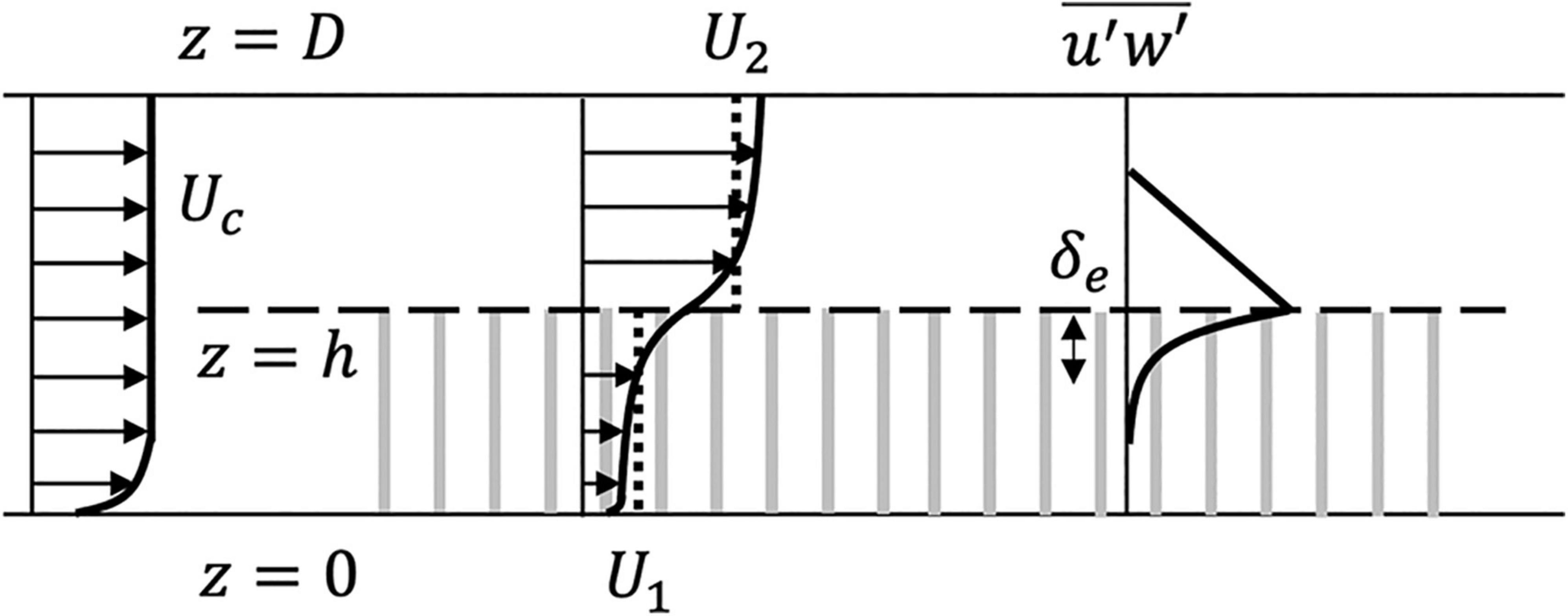
Figure 1. Simplified sketch of time-averaged velocity profiles (denoted by arrows) and Reynolds stress $\overline{u^{\prime }{w}^{\prime }}$ profile in a submerged canopy (with canopy elements represented by vertical gray rectangles). The dotted vertical lines within and above the canopy in the time-averaged velocity profiles denote the spatial vertically averaged time-averaged velocity within and above the canopy (U₁ in the canopy and U₂ above the canopy).

in which ϕ is the solid volume fraction and a_v is the frontal area per canopy volume. C_D is the canopy drag coefficient (see Supplementary Section 1 for a dictionary of symbols). C is a coefficient representing the efficiency of turbulent momentum transfer between the canopy and overflow layers:

$\begin{array}{c}\hfill C=K_c{\left(\frac{{\mathrm{\delta }}_e}{D}\right)}^{\frac{1}{3}}\hfill \end{array}(2)$

in which K_c is an empirical coefficient. For rigid canopies, Chen et al. (2013) found K_c = 0.07 ± 0.02. The penetration length scale δ_e describes the vertical distance into the canopy over which turbulent momentum flux is significant, and it is defined as the distance from the top of the canopy at which the Reynolds stress decays to 10% of the peak magnitude. The penetration length depends on the canopy height and drag length scale (C_Da_v)⁻¹, specifically ${\mathrm{\delta }}_e=min(\frac{0.23\pm 0.06}{C_D{a}_v},D-h_d,h_d)$ (Nepf and Vivoni, 2000; Konings et al., 2012). Shear is highest near the top of the canopy, such that the Reynolds shear stress $\overline{u^{\prime }{w}^{\prime }}$ reaches a peak magnitude at the canopy height (Figure 1), with u′ and w′ the velocity fluctuations in the streamwise and vertical directions, respectively, and the overbar denoting the time-averaging operation. The peak magnitude of Reynolds stress, assumed to occur at the top of the canopy, scales with the velocity difference between the overflow and canopy layers (Konings et al., 2012; Chen et al., 2013):

${\mathrm{\tau }}_{h(max)}={\mathrm{\rho }\overline{u^{\prime }{w}^{\prime }}|}_{z=h}=\mathrm{\rho }C{\left(U_2-U_1\right)}^2(3)$

in which ρ is the density of water.

In the presence of waves, Schaefer and Nepf (in review) proposed an extension to Equation 1 to account for the wave-induced current in the meadow:

$U_1=(0.6\pm 0.3){\overline{U}}_{max}+\frac{U_c}{1-\frac{h_d}{D}\varphi +\sqrt{\frac{C_D{a}_v{l}_e}{2C\left(1-\varphi \right)}{\left(\frac{D-h_d}{D}\right)}^3}}(4)$

The maximum wave-induced current ${\overline{U}}_{max}$ is (Luhar, 2021)

${\overline{U}}_{max}=\left(1.2\pm 0.2\right)U_w\sqrt{\frac{a_{v}k{l}_e}{\mathrm{\sigma }}{U}_w}(5)$

in which U_w is the wave velocity amplitude, k is the wave number, and σ is the wave angular frequency. The addition in Equation 4 assumes that the waves do not modify the momentum transfer between the meadow and overflow layers (i.e., C is effectively unchanged), and that the generation of wave-induced current is not altered by presence of an imposed current.

In addition to predicting the reduction of velocity, it is also important to predict the intensity of turbulence generated in the meadow. For unidirectional flow, a submerged meadow contributes two sources of turbulence production: shear production P_s, associated with the shear at the top of the meadow, and stem production P_w, associated with the wakes of individual stems and leaves. The shear production is

$P_s\left(z\right)=-\overline{u^{\prime }{w}^{\prime }}\frac{\partial \overline{u}}{\partial z}(6)$

in which z is the elevation above the bed and $\overline{u}$ is the time-averaged velocity. For a stem diameter d and stem density m_s (number of stems per unit bed area), the wake production is (e.g., Nepf, 2012).

$P_w\left(z\right)=\frac{1}{2}{C}_D\frac{m_{sd}}{1-\varphi }\overline{u}{(z)}^3(7)$

Averaged over the meadow height, Equation 7 is approximated as

$⟨P_w⟩=\frac{1}{2}{C}_D\frac{m_{sd}}{1-\varphi }U_1{}^3(8)$

Angle brackets indicate a canopy vertical spatial average. A prediction of TKE, k_t, is possible by equating the rates of turbulence production to the rate of turbulence dissipation, ε∼$k_t{}^{3/2}/l_t$, with l_t the turbulence integral length scale (e.g., Tennekes and Lumley, 1972). Tanino and Nepf (2008) considered this model for an array of rigid emergent cylinders, for which the shear production can be neglected. Zhang et al. (2018) extended the Tanino and Nepf (2008) model to a flexible seagrass meadow with blades of width w_b and blade density m_b (number of blades per unit bed area). For shoot spacing S > 1.8w_b, l_t∼w_b, such that ⟨P_w⟩∼ε, from which

$\frac{\sqrt{⟨k_t⟩}}{U_1}=\mathrm{\delta }{\left(C_D\frac{m_{bw}^2{}_b}{2\left(1-\varphi \right)}\right)}^{\frac{1}{3}}(9)$

The scale factor δ = 1.1 for unidirectional flow in an emergent rigid meadow, as shown in Tanino and Nepf (2008). Equation 9 with δ = 1.1 has also been validated for pure wave conditions in rigid canopies, but with the velocity scale replaced with the root-mean-squared wave velocity, U_w,RMS (Tang et al., 2019) or the wave velocity amplitude U_w (Tinoco and Coco, 2018; Chen et al., 2020). However, Zhang et al. (2018) found that the scale coefficient δ was reduced for a submerged flexible artificial seagrass meadow, and this was attributed to the motion of the blades reducing the relative velocity between the waves and the blade.

Materials and Methods

Experiments were performed in a 24 m long, 38 cm wide, and 60 cm deep laboratory flume (Figure 2). A piston-type paddle wavemaker controlled by a Syscomp WGM-101 waveform signal generator (refer to Appendix A in Luhar, 2012 for details) produced waves of period T = 2 s and varying amplitude. To reduce wave reflection, a 1:5 sloped aluminum ramp covered with rubberized coconut fiber was placed at the downstream end of the flume. The upstream edge of the ramp was lifted to allow for the passage of current. The ramp reduced wave reflection to below 11%, based on the analysis described in Goda and Suzuki (1977). Currents of varying speeds were recirculated through an inlet pipe (8 cm inner diameter) 0.8 m downstream of the wavemaker and an outlet drain downstream of the ramp.

FIGURE 2

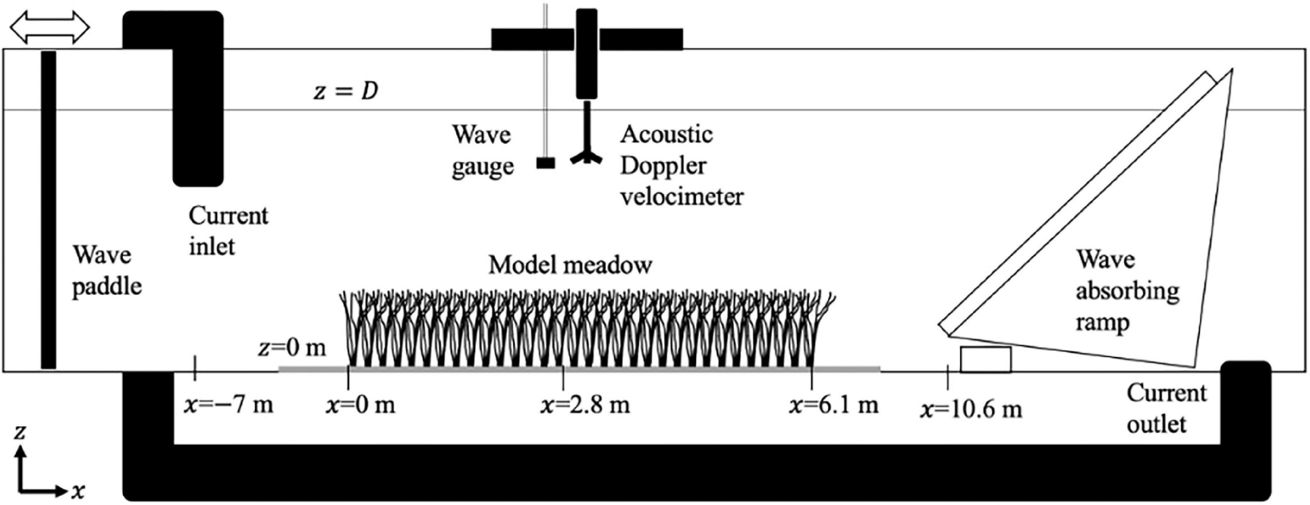
Figure 2. Sketch of experimental setup, not drawn to scale. The streamwise direction x is zero at leading edge of the model meadow, and the vertical direction z is zero at the bed and positive upward.

Construction of Artificial Seagrass Shoot and Meadow

A seagrass shoot model was constructed to be geometrically and dynamically similar to Zostera marina (e.g., Ghisalberti and Nepf, 2002). Each model shoot had six blades laser-cut from low-density polyethylene (LDPE). Each blade was 13 cm long, 0.3 cm wide, and 0.1 mm thick. The blades were wrapped around the upper half of a 0.6 cm diameter, 1.3 cm long cylindrical dowel using tape, which increased the diameter by 0.1 cm. The erect height of each shoot was h = 13.6 cm.

The shoots were inserted in a staggered pattern into pre-drilled holes in polyvinyl chloride boards such that the rigid dowels, representing the seagrass sheaths, extended 0.6 cm above the baseboards. The shoot density m_s = 950 shoots per square meter, and the blade density m_b = 5,700 blades per square meter. A bare baseboard (1.2 m in length) was placed at the upstream and downstream ends of the 6.1 m long meadow. Experiments were performed with mean water depths D = 27 cm and 45 cm above the baseboards. For each water depth, four pure wave cases, four pure current cases, and sixteen combined wave-current cases were considered (see Supplementary Section 2). Turbulence generated at the current inlet slightly modified the wave amplitude relative to pure wave conditions with the same wavemaker setting.

Velocity Measurements, Wave Gauge Measurements, and Meadow Imaging

The velocities in the streamwise (x), lateral (y), and vertical (z) directions were defined as (u,v,w), respectively. Instantaneous velocities were measured with a Nortek Vectrino three-dimensional acoustic velocimeter, which was centered longitudinally between successive shoot rows and laterally between adjacent shoots, at the spanwise center of the flume. This position within a staggered array has been shown to offer accurate estimates of the laterally averaged velocity and turbulence in current and wave conditions (see Figure 2 in Chen et al., 2013 and Figure 2 in Zhang et al., 2018). To minimize interference with the measurement volume, blades were removed from shoots within a 10 cm diameter circle around the probe (see Luhar et al., 2010). Measurements were taken along a vertical transect in 1 cm intervals above the bed at the longitudinal center of the meadow (x = 2.8 m), for 240 s at 200 Hz for each case.

Velocity records were cleaned using the acceleration thresholding methods described in Goring and Nikora (2002). Each component of velocity was decomposed into the summation of the time-averaged (denoted by an overbar), phase-averaged (denoted by a tilde), and turbulent (denoted by prime) velocity. For example, for the streamwise component,

$u(t,z)=\overline{U}\left(z\right)+\tilde{U}(t,z)+u^{\prime }(t,z)(10)$

in which t is time. The number of samples n_s in each wave period was estimated through autocorrelation. The phase-averaged velocity $\tilde{U}\left(\mathrm{\theta }\right)$ was calculated for each of the n_s=403 phase bins, in which θ is the wave phase. The time-averaged velocity was calculated as

$\overline{U}=\frac{1}{2\mathrm{\pi }}{\int }_0^{2\mathrm{\pi }}\tilde{U}\left(\mathrm{\theta }\right)\mathit{d}\mathrm{\theta }(11)$

The depth-averaged imposed current U_c was defined by integrating $\overline{U}$ over depth upstream of the meadow. The time-averaged TKE was calculated as

$TKE=\frac{1}{4\mathrm{\pi }}{\int }_0^{2\mathrm{\pi }}\left[u_{RMS}^{\prime }{\left(\mathrm{\theta }\right)}^2+v_{RMS}^{\prime }{\left(\mathrm{\theta }\right)}^2+w_{RMS}^{\prime }{\left(\mathrm{\theta }\right)}^2\right]\mathit{d}\mathrm{\theta }(12)$

Water surface displacement η was measured with a wave gauge (1,000 Hz for 90 s) at the longitudinal center of the meadow, which provided both the wave amplitude and confirmed stationary wave conditions. The wave-to-wave variation in wave amplitude was less than 1% of the phase-averaged wave amplitude, determined using $\frac{1}{2\mathrm{\pi }}{\int }_0^{2\mathrm{\pi }}{\mathrm{\eta }}_{RMS}\left(\mathrm{\theta }\right)\mathit{d}\mathrm{\theta }/{\mathrm{\eta }}_{w,RMS}$, as described in Zhang et al. (2018). This indicated that the variation in wave form made negligible impact on the estimation of the turbulence within the phase-averaged method (Equation 12).

The in-canopy velocity U₁ for each case was estimated as a vertical average of the time-mean velocity between the bed and the time-mean deflected canopy height, h_d. Mean deflected heights were estimated from digital videos of six blades painted black at the longitudinal center of the meadow collected using a Nikon D7500 camera. The videos were viewed and processed using MATLAB VideoReader, readFrame, and Sobel edge detection functions. A red-green-blue pixel identification algorithm was used to identify the painted blades. The vertical positions of the highest and lowest part of each blade were recorded for all cases under the wave crests and troughs. The mean deflected canopy height h_d was defined as the average across all six blades. The characteristic wave velocity amplitude U_w for each case was defined from Stokes second-order wave theory under the crest (LeMéhauté, 1976; Dean and Dalrymple, 1984) at the undeflected canopy height (z=h) using the measured wave amplitude at x = 2.8 m, the location of mid-meadow velocity measurements.

Drag Coefficient

The drag coefficient C_D for the flat rectangular blades was assumed to be 1.95 (as in Zhang et al., 2018). Zhang et al. (2018) found that using a variable C_D to account for the impact of different hydrodynamic conditions on blade reconfiguration did not improve TKE predictions, as the drag coefficient used in TKE predictions represents the drag along the vertical part of the plant. Furthermore, although Sarpkaya and Storm (1985) observed that the addition of a current to oscillatory flow could alter the drag coefficient, the impact depended on the Keulegan-Carpenter number KC=U_wT/w_b (Keulegan and Carpenter, 1958). They observed that the drag coefficients of cylinders in combined wave-current conditions converged for KC > 15, and the impact of current on drag coefficients became negligible for KC > 30. In this study all KC were greater than 24. Based on this, and for simplicity, in this study the drag coefficient in pure current, pure wave, and wave-current conditions was assumed to be 1.95.

Results

Time-Averaged Velocity Profiles

Selected profiles of time-averaged velocity were used to illustrate the flow behavior (Figure 3), including the strongest imposed current in both depths. The full set of profiles is given in Supplementary Section 3. See Supplementary Section 2 for details of all conditions. For pure current cases (red triangles in Figure 3), the time-averaged velocity profiles included a mixing-layer at or just above the meadow interface and a peak velocity well above the meadow (Figures 3A,D). Wave-current cases (circles in Figure 3) with U_w/U_c < 2.5 retained this mixing-layer time-mean structure, but the center of the shear layer moved toward the bed as either the imposed current or wave velocity was increased, both of which were associated with a reduction in the canopy deflected height (horizontal dashed lines in Figure 3; see Supplementary Section 4).

FIGURE 3

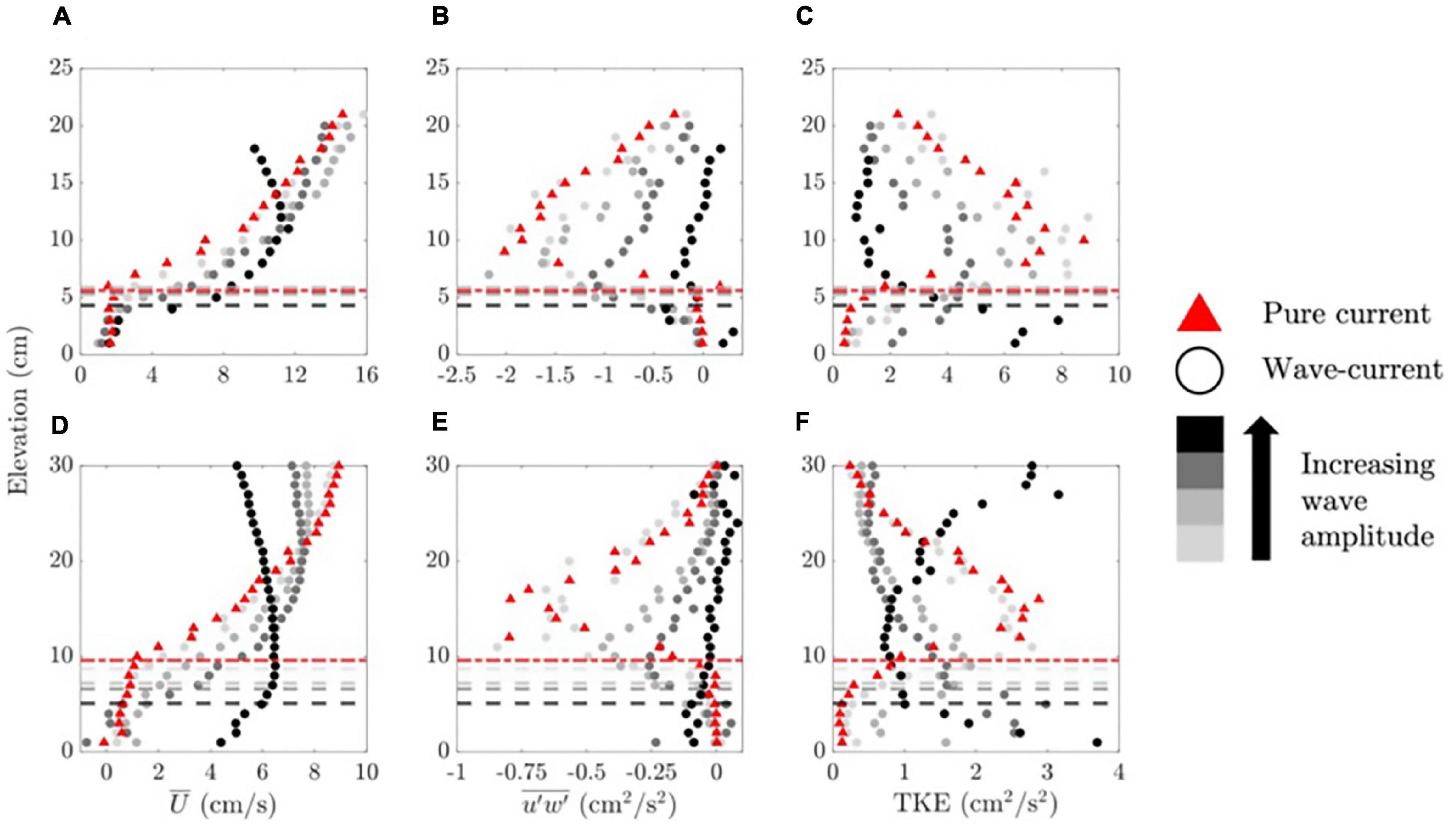
Figure 3. Distance above the bed (z) vs. (A,D) time-averaged velocity ($\overline{U}$), (B,E) Reynolds stress ($\overline{u^{\prime }{w}^{\prime }}$), and (C,F) TKE for the largest imposed current and all waves for cases with (A–C) depth D = 27 cm and (D–F) depth D = 45 cm. In panels (A–C), U_c = 10.4 cm s^–1 and U_w = 3.2–4.7 cm s^–1 (lightest gray), U_w = 4.1–7.4 cm s^–1 (second-lightest gray), U_w = 8.9–10.0 cm s^–1 (second-darkest gray), and U_w = 19.2–21.8 cm s^–1 (black). In panels (D–F), U_c = 6.8 cm s^–1 and U_w = 2.9–3.9 cm s^–1 (lightest gray), U_w = 8.1–8.8 cm s^–1 (second-lightest gray), U_w = 10.1–11.1 cm s^–1 (second-darkest gray), and U_w = 15.4–19.0 cm s^–1 (black) (turbulence at the current inlet pipe slightly modified wave amplitudes for higher currents relative to pure wave conditions for the same programmed wave). Horizontal dashed lines denote measured h_d, with matching colors (dashed-dotted lines correspond to pure current). Profiles could not be extended over the entire depth due to limitations of the instrument and the presence of waves. Profiles for cases with depth D = 45 cm are shortened to 30 cm to show detail within and above the canopy.

For most cases with U_w/U_c > 2.5, the time-mean velocity peaked at the top of the canopy, reflecting the contribution from the wave-induced current (discussed in Section “Theoretical Background for Predicting Velocity and Turbulence in Meadow” and predicted with Equation 5), so that these conditions were considered to be wave-dominated. The transition at approximately U_w/U_c=2.5 is supported by Figure 4, which illustrates the distribution of cases for which the time-averaged velocity peaked at the top of the canopy (wave-dominated, triangles) or for which the time-averaged velocity peaked above the canopy (circles). The transition was not a function of current Reynolds number (U_cD/ν, in which ν is the kinematic viscosity of water). Finally, for the largest waves (black circles in Figure 3), the time-averaged current was reduced near the water surface. This was attributed to a wave-induced Eulerian drift, which has been observed in several previous studies in laboratory water channels and in the field (Nepf et al., 1995; Gjøsund, 2003; Smith, 2006; Monismith et al., 2007).

FIGURE 4

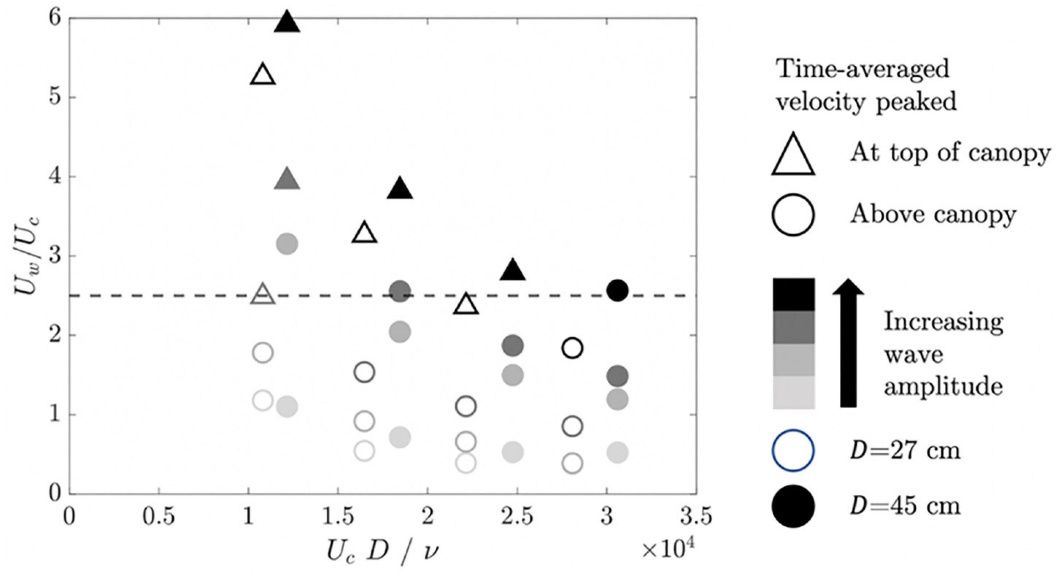
Figure 4. Wave-to-current velocity ratio (U_w/U_c) vs. current Reynolds number (U_cD/ν). Circles denote cases for which the time-averaged velocity peaked above the canopy, similar to pure current conditions. Triangles denote cases for which the time-averaged velocity peaked at the top of the canopy, indicating that the wave-induced mean current was significant within the meadow.

Reynolds Stress and Turbulent Kinetic Energy Profiles

For pure current (red triangles in Figures 3B,E) and wave-current (circles in Figures 3B,E) cases with a clear mixing layer flow structure, the magnitude of the Reynolds stress was approximately zero near the bed, increased to a peak near the mean deflected meadow height (dashed horizontal lines in Figure 3), and then decreased with distance above the meadow. As the wave amplitude increased, the peak Reynolds stress magnitude decreased (Figures 3B,E). A peak in TKE appeared near the top of the canopy (Figures 3C,F), coincident with the peak in Reynolds stress, which was consistent with shear production (Equation 6). As the wave amplitude increased, this TKE peak was diminished, consistent with the decrease in Reynolds stress peak magnitude. The opposite trend was observed within the canopy. Specifically, as wave amplitude increased, TKE within the canopy increased (see the progression of light gray to darker gray to black symbols below the dashed lines in Figures 3C,F), reflecting the contribution of wake production, which increased with the addition of waves. For larger waves, TKE in the upper water column increased toward the water surface (e.g., black circles in Figure 3F). The near-surface enhancement in TKE was attributed to a secondary circulation. Specifically, the interaction between progressive waves and vertical vorticity, here associated with the side-wall boundary layers, generated a secondary circulation by Langmuir instability, with downwelling at the channel center (Nepf and Monismith, 1991). This circulation elevates near-surface turbulence (Nepf et al., 1995).

Prediction of Magnitude of Peak Reynolds Stress

The addition of waves had little impact on the magnitude of peak Reynolds stress for U_w/U_c < 1, but for U_w/U_c > 1 the peak Reynolds stress magnitude decreased with increasing wave amplitude, compared to the corresponding pure current conditions (Figure 5A; also see the Reynolds stress profiles in Supplementary Figures 3.1, 3.2, noting the change in magnitude of the maximum Reynolds stress with increasing wave amplitude for each current). The reduction in Reynolds stress was predominantly associated with a decrease in velocity shear, rather than a change in the efficiency in turbulent momentum transport. This distinction was illustrated by considering the idealized two-layer model for canopy flow, which defines the Reynolds stress at the top of the meadow, τ_h(max), in terms of the layer-averaged time-averaged velocity within, U₁, and above, U₂, the meadow (Equation 3). When the momentum coefficient C (=0.014–0.020) was estimated using Equation 2, then Equation 3 predicted the maximum magnitude of Reynolds stress within uncertainty (Figure 5B) for both pure current cases and the wave-current cases that exhibited shear layer behavior, indicating that the momentum coefficient was not significantly changed by the waves.

FIGURE 5

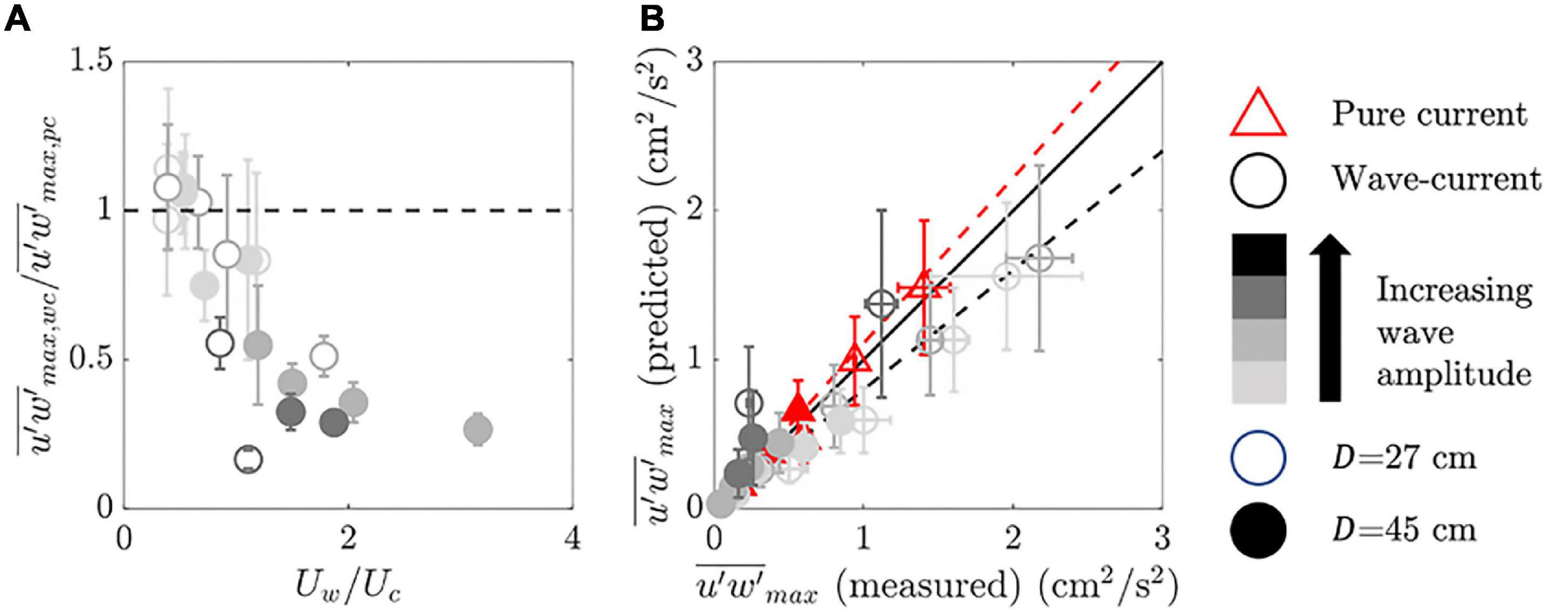
Figure 5. (A) Maximum magnitude of Reynolds stress in combined wave-current (subscript “wc”) conditions (${\overline{u^{\prime }{w}^{\prime }}}_{max,wc}$) normalized by the maximum magnitude of Reynolds stress in corresponding pure current (subscript “pc”) conditions (${\overline{u^{\prime }{w}^{\prime }}}_{max,pc}$) vs. wave-to-current velocity ratio (U_w/U_c). (B) Predicted vs. measured maximum magnitude of Reynolds stress (${\overline{u^{\prime }{w}^{\prime }}}_{max}$). Cases that showed a shear layer flow structure were included. The dashed line in panel (A) denotes a ratio of 1. The red and black dashed lines in panel (B) denote the lines of best fit for pure current (red triangles) and combined wave-current (circles) cases, respectively. The solid black line in panel (B) is a one-to-one line. Error bars in panel (A) indicate uncertainties assessed using propagated uncertainties in the ratio of measured maximum magnitudes of Reynolds stress (single point measurements, using half of their range when the record was split in half) and in panel (B) indicate propagated uncertainties in the prediction of the maximum magnitude of Reynolds stress [from C (Equation 2), as well as U₂ and U₁ (in which the mean deflected height h_d measurements were the dominant source of uncertainty) in Equation 3].

However, note that the best fit line through the combined wave-current cases (black dashed line fitted to circles in Figure 5B, ${\overline{u^{\prime }{w}^{\prime }}}_{max}\left(predicted\right)=\left(0.80\pm 0.09\right){\overline{u^{\prime }{w}^{\prime }}}_{max}\left(measured\right)$) fell below that for the pure current cases (red dashed line fitted to triangles in Figure 5B, ${\overline{u^{\prime }{w}^{\prime }}}_{max}\left(predicted\right)=\left(1.11\pm 0.07\right){\overline{u^{\prime }{w}^{\prime }}}_{max}\left(measured\right)$), which suggested that Equation 2 underpredicted C by 20–30% for combined wave-current cases. This trend suggested that the presence of waves augmented the vertical turbulent transfer of momentum. However, this conclusion is only speculative, because in fact Equation 3 produced predictions consistent with the measured stress. The trends in Figure 5 can be explained as follows. The addition of waves reduced h_d, relative to pure current conditions, which increased the depth of overflow (D−h_d), which in turn decreased U₂. The reduction in U₂−U₁ led to a decrease in Reynolds stress. Because the efficiency of turbulent momentum change was not significantly altered (C was the same within uncertainty), the decrease in Reynolds stress was consistent with the decrease in velocity gradient (Figure 5B). It is important to note that if C is not impacted by waves (as suggested here), then two-layer models developed for pure current conditions can be used to predict the in-canopy velocity in combined wave-current conditions, using the deflected height (i.e., Equation 4), which is supported by analysis in Schaefer and Nepf (in review). This is a useful result for modeling flows through submerged meadows.

Canopy Turbulent Kinetic Energy Measurements and Predictions

The canopy-averaged shear production ⟨P_s⟩ of turbulence was estimated by averaging Equation 6 over the deflected canopy height. The canopy-averaged wake production ⟨P_w⟩ of turbulence was estimated from Equation 7 using the in-canopy depth-averaged, time-averaged velocity, U₁. This represents a lower bound on wake production, because $⟨\overline{u}{(z)}^3⟩>U_1{}^3$, and contributions from wave velocity were neglected. Even using an underestimate for ⟨P_w⟩, the ratio ⟨P_w⟩/⟨P_s⟩ was greater than five for all but three cases and greater than 10 for all but eight cases (see Supplementary Section 4). Given this, it was reasonable to neglect the shear-production and thus to expect a form of Equation 8 to predict TKE within the canopy. However, we must determine the appropriate velocity scale for TKE prediction.

For combined wave-current conditions, Chen et al. (2020) proposed that stem-generated turbulence scaled with the sum of the wave velocity and imposed depth-averaged current velocity, i.e., with the maximum velocity in the wave period, U_max. Within a rigid submerged meadow, they observed a linear relationship between TKE and $U_{max}^2$. Here, we considered a similar relationship in a flexible canopy, using the sum of the wave velocity U_w and in-canopy depth-averaged, time-averaged velocity U₁. Recall that in the presence of waves, a wave-induced current will augment U₁ above the imposed current velocity (see Equation 4). Specifically, we considered the dependence of TKE and (U_w+U₁)², as shown in Figure 6.

FIGURE 6

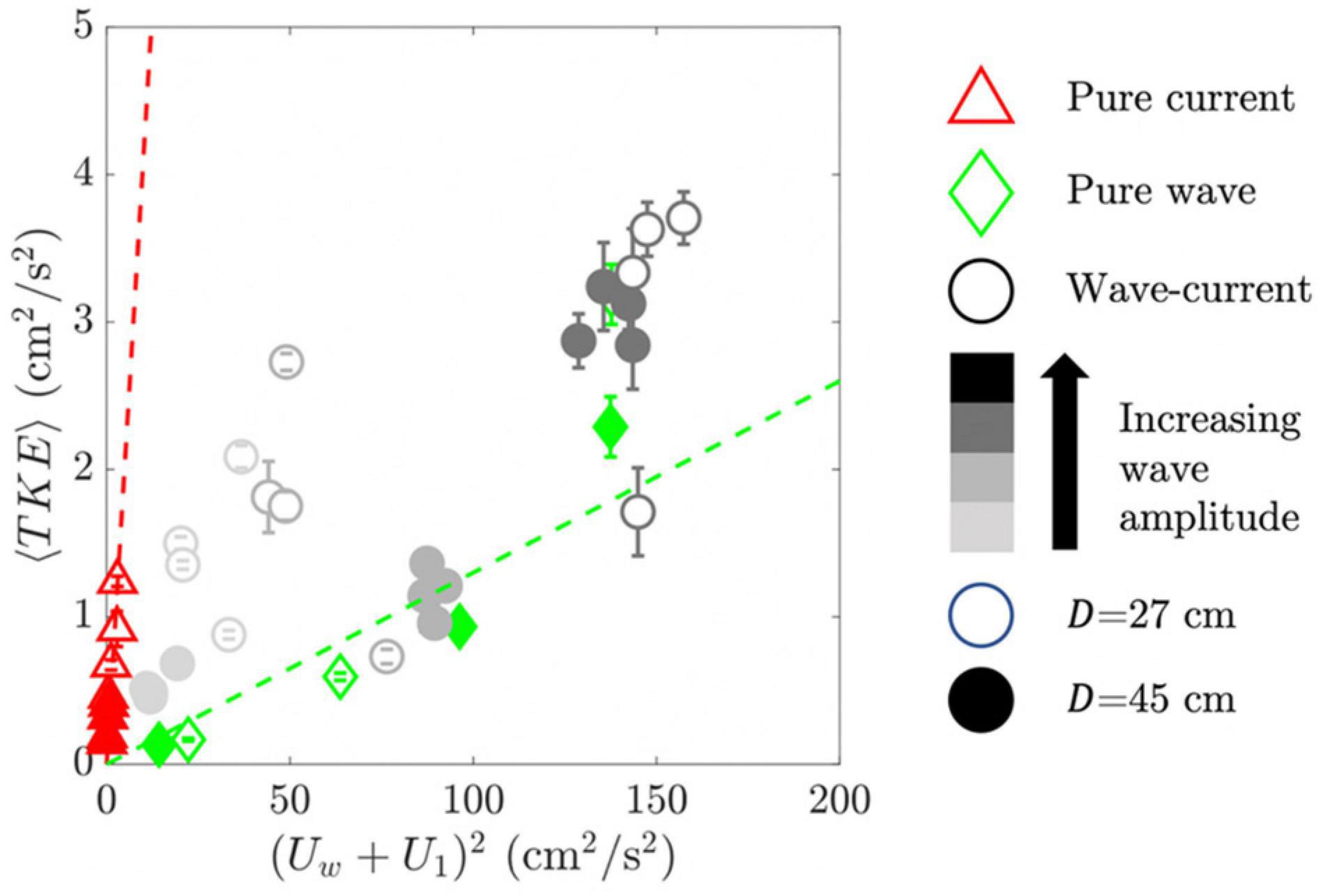
Figure 6. Measured canopy-averaged TKE (⟨TKE⟩) vs. the squared sum of the wave velocity and the in-canopy depth-averaged, time-averaged velocity ((U_w+U₁)²). Red and green dashed lines denote best fit lines for pure current and pure wave cases, respectively. For clarity among the cases with smaller TKE, the highest TKE cases were excluded (see Figure 7). Error bars indicate uncertainties assessed in the canopy-averaged TKE (propagating uncertainties using half of the range from each measurement when the records were split in half).

First, note that there was a stronger dependence between TKE and velocity for pure current (red triangles in Figure 6) than for pure waves (green diamonds in Figure 6). Specifically, using the velocity scale (U_w+U₁) in Equation 9, the scale factor for pure current, δ_pc=1.8 ± 0.3, was six times larger than for pure wave (δ_pw=0.30 ± 0.04). This makes physical sense, because flexible blades can move with the wave orbital velocity, which reduces the relative velocity, the drag, and the wake turbulence production Zhang et al. (2018). In pure current, the flexibility can allow plants to become more streamlined, but it cannot reduce the relative velocity. Zhang et al. (2018) also observed a smaller scale factor in Equation 9 for flexible blades under pure wave conditions. Specifically, using velocity scale U_w,RMS in Equation 9 they found δ_pw=0.44, which converts to δ_pw=0.22 for the velocity scale U_w, as used here. Note that the pure current scale factor δ_pc was larger than the scale factor 1.1 found for rigid emergent cylinders (Tanino and Nepf, 2008), which may be explained by the difference in morphology between emergent cylinders and submerged model plants. First, Equation 9 assumes that the integral length scale is equal to the blade width, l_t=w_b, which may not be appropriate in the lower canopy, where the blades are bundled into a sheath of larger dimension (sheath diameter = 0.7 cm), or near the top of the canopy where larger shear layer vortices are present (Poggi et al., 2004; Zhang et al., 2020). Second, Equation 9 uses the canopy-averaged velocity U₁. However, for a submerged meadow the velocity varies over the canopy height, and $U_1{}^2$ will underestimate $⟨\overline{u}{(z)}^2⟩$, and this must be offset by a larger scale coefficient.

Next, consider the combined wave-current cases (gray to black circles in Figure 6), which predominantly fell in between the dependences observed for pure current (red triangles) and pure wave (green diamonds). This suggested that a simple hybrid wake production model might collapse all of the cases. Specifically, we proposed the following modification to Equation 9 for wave-current conditions ⟨k_t,wc⟩:

$⟨k_{t,wc}⟩={\left(C_D\frac{m_{bw}^2{}_b}{2\left(1-\varphi \right)}\right)}^{\frac{2}{3}}\left({\mathrm{\delta }}_{pc}^{2}U_1{}^2+{\mathrm{\delta }}_{pw}^{2}U_w{}^2\right)(13)$

Indeed, this hybrid model collapsed most of the data (Figure 7).

FIGURE 7

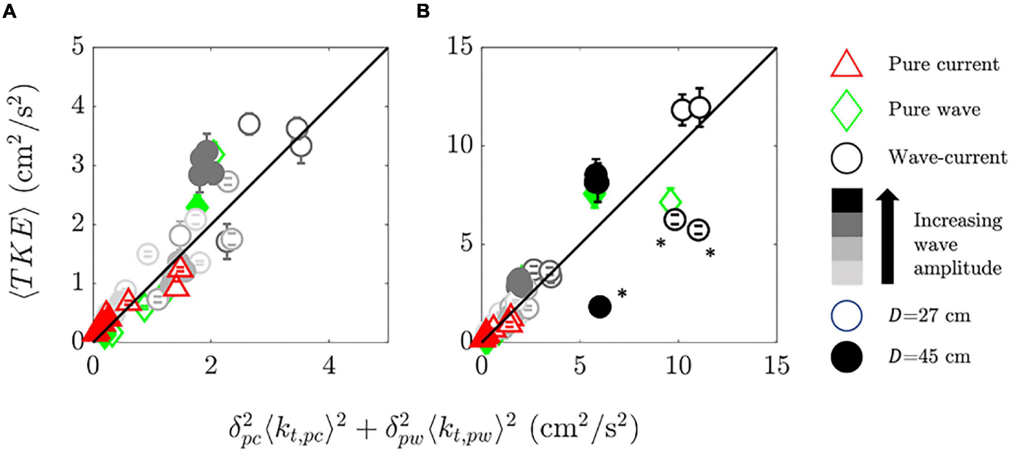
Figure 7. Measured canopy-averaged TKE (⟨TKE⟩) vs. the proposed hybrid model (${\mathrm{\delta }}_{pc}^2⟨k_{t,pc}⟩+{\mathrm{\delta }}_{pw}^2⟨k_{t,pw}⟩$, Equation 13) with (A) axes scaled to highlight that the majority of cases collapse reasonably well by the hybrid model and (B) showing all cases. The solid black lines denote one-to-one lines. In panel (B), asterisks denote cases involving the highest waves, but atypically low TKE, as discussed in Section “Blade Reconfiguration and Wake Production” in the text. Error bars indicate uncertainties assessed in canopy-averaged TKE (as in Figure 7).

As an alternative to the hybrid model, it would be useful to evaluate when the canopy turbulence is dominated by either the current or the waves, allowing for prediction of ⟨k_t⟩ using only the wave or current velocity. Consider the ratio of canopy-averaged turbulence in wave-current conditions ⟨TKE_wc⟩ normalized by corresponding TKE in pure current ⟨TKE_pc⟩ and pure wave ⟨TKE_pw⟩ vs. U_w/U_c, as shown in Figure 8. For U_w/U_c < 1, increasing U_w/U_c had minimal impact on canopy turbulence relative to pure current conditions, compared to the increase in TKE observed with increasing U_w/U_c for U_w/U_c > 1 (Figure 8A). Alternatively, when current was added to waves, ⟨TKE_wc⟩/⟨TKE_pw⟩ was greater than 1 for U_w/U_c < 1, but converged to 1 for U_w/U_c > 1 (Figure 8B). Together, these trends suggest that for U_w/U_c > 1, a good prediction of TKE can be made using just the wave velocity. Conversely, for U_w/U_c < 1, a good prediction of TKE can be made using just the current velocity.

FIGURE 8

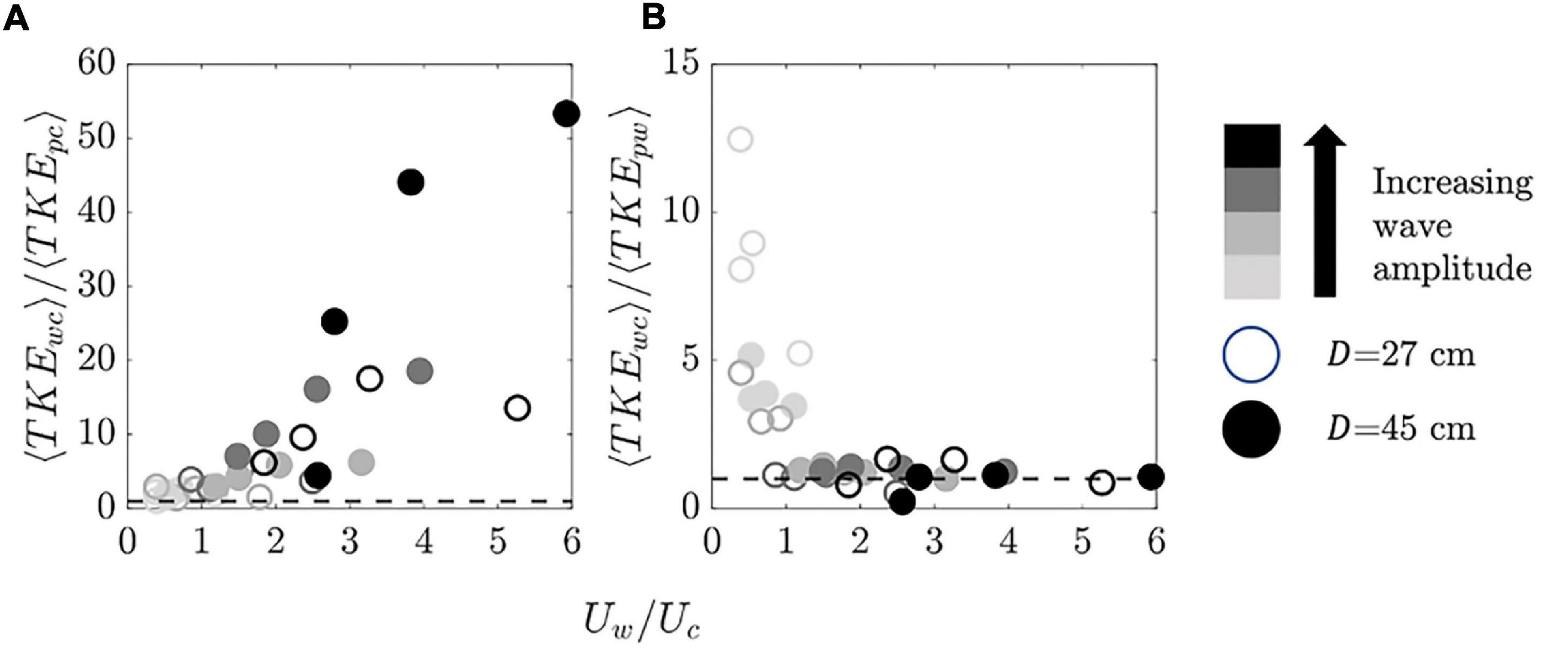
Figure 8. Canopy-averaged turbulent kinetic energy in wave-current (subscript “wc”) conditions (⟨TKE_wc⟩) normalized by (A) canopy-averaged TKE in pure current (subscript “pc”) conditions (⟨TKE_pc⟩) and (B) canopy-averaged TKE in pure wave (subscript “pw”) conditions (⟨TKE_pw⟩), both vs. the wave-to-current velocity ratio (U_w/U_c). The dashed horizontal lines are (A) ⟨TKE_wc⟩/⟨TKE_pc⟩=1 and (B) ⟨TKE_wc⟩/⟨TKE_pw⟩=1.

Discussion

Laboratory experiments with an artificial seagrass meadow described the impact of waves on the time-averaged velocity, Reynolds stress, and TKE within a flexible submerged meadow. The study considered a range of wave and current conditions for a single meadow density (950 shoots m^–2, 5,700 blades m^–2). One major result of this study is that for a flexible meadow, wave velocity is less efficient in generating TKE (smaller scale coefficient), because wave-induced motion of the blades reduces the relative velocity between the blade and the waves. The resultant proposed hybrid model (Equation 13) is valid when wake production dominates shear production. Overall, this study provided important validation of models that predict Reynolds stress and turbulence within a submerged meadow in realistic conditions of combined waves and currents. These models provide a quantitative framework to predict ecosystem services facilitated by meadow-mediated hydrodynamic conditions.

Impact of Waves on Mean Deflected Height

The observed reduction in h_d in the presence of waves contrasted with observations in Paul and Gillis (2015), who observed that for combined wave and current conditions, the presence of a wave did not appear to impact the mean deflected canopy height. The discrepancy might be related to the fact that Paul and Gillis (2015) used the tip of the blade to estimate the canopy height, while the present study considered the highest position along the length of the blade. The pronation of blades in the direction of wave propagation, resulting in a decrease in mean deflected height, has been observed in previous studies and attributed to two mechanisms. First, observations showed that the vertical component of the wave orbital velocity induced asymmetric blade motion and deflection in the direction of wave propagation (Döbken, 2015). Second, the wave-induced current generated in the meadow can pronate the individual blades (Zhang et al., 2018).

Reynolds Stress at the Top of the Canopy

The direct contribution of waves to shear and turbulent momentum exchange (i.e., Reynolds stress) at the top of the canopy is limited to long period waves, as described in Ghisalberti and Schlosser (2013). They defined a wave Reynolds number, Re_w=2U_wd/πν, and a Keulegan-Carpenter number KC_s as the ratio of wave period to the time scale of vortex formation. Specifically, KC_s=U_wT/L_D, with L_D=2(C_Da_v)⁻¹(1−ϕ) (e.g., Chen et al., 2013). Pure waves can generate vortices at the top of a canopy only when both KC_s > 5 and Reynolds number Re_w > 1,000. For the meadow in the present study, KC_s < 2.2 and Re_w < 600, indicating that the waves did not contribute to Reynolds stress or shear production at the top of the canopy, consistent with the fact that C was not impacted by the addition of waves.

In addition, note that the peak Reynolds stress did not always occur at the mean deflected height, but for most cases occurred within a few cm above the mean deflected height. This was in contrast to measurements in unidirectional flow made for a flexible meadow of lower density (230 shoot m^–2), for which the peak Reynolds stress was consistently at the canopy interface (Ghisalberti and Nepf, 2006). The shoot density in the present study was much higher at 950 shoot m^–2, which may have reduced the shear penetration into the canopy, pushing the shear layer and peak Reynolds stress slightly above the canopy interface. Considering the measured maximum deflected height instead of the measured mean deflected height, as in Ghisalberti and Nepf (2006), did not explain the slightly shifted position of the Reynolds stress peak.

Blade Reconfiguration and Wake Production

For the three wave-current cases marked with asterisks in Figure 7, the canopy-averaged turbulence was noticeably lower than other wave-current cases of the same programmed wave amplitude and depth. Cases of the highest wave amplitudes had the smallest deflected heights (see Supplementary Section 4), with many blades touching the bed during the wave period (see the conceptual sketch in Figure 9). It was possible that the blades, which were in-line with the sheath, restricted flow around the sheath, which reduced or eliminated the shedding of vortices from the sheath for the marked cases. This is a potentially important observation, as it illustrates how wake turbulence can be eliminated when the meadow pronation due to reconfiguration becomes extreme. While this description does not fully explain the differences in canopy TKE among all of the strongest wave cases, it was likely a contributing factor.

FIGURE 9

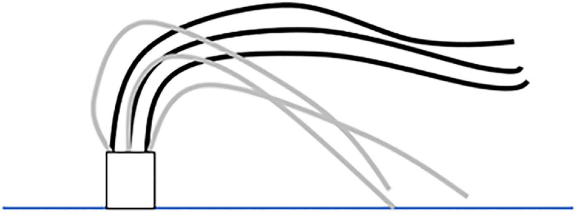
Figure 9. Conceptual sketch of the side view of a model seagrass plant showing blade motion under a wave crest (black curves) and wave trough (gray curves), corresponding to the strongest wave forcing (e.g., black circles in Figure 7). The rectangle represents the sheath.

Relative Strengths of Wave and Current Velocities

For clarity, we note that the aforementioned threshold of approximately U_w/U_c=2.5 described changes in the time-mean velocity profile. Specifically, the time-mean velocity peaked above the canopy when U_w/U_c < 2.5, and peaked at the top of the canopy when U_w/U_c > 2.5. Meanwhile, shifts in canopy turbulence were observed at a lower threshold U_w/U_c=1. Combining these, when 1 < U_w/U_c < 2.5, the wave velocity dominated the production of TKE in the canopy, but did not significantly modify the current-induced time-mean flow structure behavior. We note that these transitions may have some dependence on canopy density, which was not explored in the present study. Finally, seagrass meadows exhibit a wide range of density (140–30,000 blades per bed area; see Table 3 in Luhar et al., 2010), both more and less dense than the model canopy considered in this study (5,700 blades m^–2). The assumption that wake production dominates shear production, which was validated in the present study, likely extends to denser meadows, but may not be valid in sparser meadows.

Data Availability Statement

The raw data supporting the conclusions of this article will be made available by the authors, without undue reservation.

Author Contributions

HN and RS conceptualized the project and contributed to writing the draft. RS conducted the experiments and data processing. HN provided the laboratory space and equipment. Both authors contributed to the article and approved the submitted version.

Funding

This material is based upon work supported by the National Science Foundation under Grant No. 1659923 and the National Science Foundation Graduate Research Fellowship under Grant No. 1745302. RS was supported in part by the Louis Berger Fellowship Fund in the Massachusetts Institute of Technology Department of Civil and Environmental Engineering.

Conflict of Interest

The authors declare that the research was conducted in the absence of any commercial or financial relationships that could be construed as a potential conflict of interest.

Publisher’s Note

All claims expressed in this article are solely those of the authors and do not necessarily represent those of their affiliated organizations, or those of the publisher, the editors and the reviewers. Any product that may be evaluated in this article, or claim that may be made by its manufacturer, is not guaranteed or endorsed by the publisher.

Supplementary Material

The Supplementary Material for this article can be found online at: https://www.frontiersin.org/articles/10.3389/fmars.2022.836901/full#supplementary-material

References

Brunet, Y., Finnigan, J. J., and Raupach, M. R. (1994). A wind tunnel study of air flow in waving wheat: single-point velocity statistics. Boundary Layer Meteorol. 70, 95–132. doi: 10.1007/BF00712525

CrossRef Full Text | Google Scholar

Chen, M., Lou, S., Liu, S., Ma, G., Liu, H., Zhong, G., et al. (2020). Velocity and turbulence affected by submerged rigid vegetation under waves, currents and combined wave-current flows. Coast. Eng. 159:103727. doi: 10.1080/10643389.2012.728825

CrossRef Full Text | Google Scholar

Chen, Z., Jiang, C., and Nepf, H. M. (2013). Flow adjustment at the leading edge of a submerged aquatic canopy. Water Resour. Res. 49, 5537–5551. doi: 10.1002/wrcr.20403

CrossRef Full Text | Google Scholar

Cheng, N. S. (2011). Representative roughness height of submerged vegetation. Water Resour. Res. 47, 1–18. doi: 10.1029/2011WR010590

CrossRef Full Text | Google Scholar

Dean, R. G., and Dalrymple, R. A. (1984). Water Wave Mechanics for Engineers and Scientists. Englewood Cliffs, NJ: Prentice-Hall.

Google Scholar

Döbken, J. W. D. (2015). Modeling the Interaction of Wave Hydrodynamics with Flexible Aquatic Vegetation. Master’s thesis. Delft: Delft University of Technology.

Google Scholar

Fonseca Cahalan, J. A. (1992). A preliminary evaluation of wave attenuation by four species of seagrass. Estuar. Coast. Shelf. Sci. 35, 565–576. doi: 10.1016/S0272-7714(05)80039-3

CrossRef Full Text | Google Scholar

Fonseca Koehl, M. A. R., and Kopp, B. S. (2007). Biomechanical factors contributing to self-organization in seagrass landscapes. J. Exp. Mar. Biol. Ecol. 340, 227–246. doi: 10.1016/j.jembe.2006.09.015

CrossRef Full Text | Google Scholar

Fonseca, M. S., Fisher, J. S., Zieman, J. C., and Thayer, G. W. (1982). Influence of the seagrass, Zostera marina L., on current flow. Estuar. Coast. Shelf. Sci. 15, 351–364. doi: 10.1016/0272-7714(82)90046-4

CrossRef Full Text | Google Scholar

Ghisalberti, M., and Nepf, H. M. (2002). Mixing layers and coherent structures in vegetated aquatic flows. J. Geophys. Res. 107, 3–1. doi: 10.1029/2001jc000871

CrossRef Full Text | Google Scholar

Ghisalberti, M., and Nepf, H. M. (2006). The structure of the shear layer in flows over rigid and flexible canopies. Environ. Fluid Mech. 6, 277–301. doi: 10.1007/s10652-006-0002-4

CrossRef Full Text | Google Scholar

Ghisalberti, M., and Schlosser, T. (2013). Vortex generation in oscillatory canopy flow. J. Geophys. Res. Oceans 118, 1534–1542. doi: 10.1002/jgrc.20073

CrossRef Full Text | Google Scholar

Gillis, L. G., Paul, M., and Bouma, T. (2017). Ammonium uptake rates in a seagrass bed under combined waves and currents. Front. Mar. Sci. 4:207. doi: 10.3389/fmars.2017.00207

CrossRef Full Text | Google Scholar

Ginsburg, R., and Lowenstam, H. (1958). The influence of marine bottom communities on the depositional environment of sediments. J. Geol. 66, 310–318. doi: 10.1086/626507

CrossRef Full Text | Google Scholar

Gjøsund, S. H. (2003). A Lagrangian model for irregular waves and wave kinematics. J. Offshore Mech. Arct. Eng. 125, 94–102. doi: 10.1115/1.1554702

CrossRef Full Text | Google Scholar

Goda, Y., and Suzuki, Y. (1977). “Estimation of incident and reflected waves in random wave experiments,” in Proceedings of the 15th Coastal Engineering Conference, Honolulu, HI, 828–845. doi: 10.9753/icce.v15.47

CrossRef Full Text | Google Scholar

Goring, D. G., and Nikora, V. I. (2002). Despiking acoustic doppler velocimeter data. J. Hydraul. Eng. 128, 117–126. doi: 10.1061/(ASCE)0733-94292002128:1(117

CrossRef Full Text | Google Scholar

Homziak, J., Fonseca, M., and Kenworthy, W. (1982). Macrobenthic community structure in a transplanted eelgrass (Zostera marina) meadow. Mar. Ecol. Progr. Ser 9, 211–221. doi: 10.3354/meps009211

CrossRef Full Text | Google Scholar

Huthoff, F., Augustijn, D. C. M., and Hulscher, S. J. M. H. (2007). Analytical solution of the depth-averaged flow velocity in case of submerged rigid cylindrical vegetation. Water Resour. Res. 43, 1–10. doi: 10.1029/2006WR005625

CrossRef Full Text | Google Scholar

Keulegan, G. H., and Carpenter, L. H. (1958). Forces on cylinders and plates in an oscillating fluid. J. Res. Natl. Bur. Stand. 60:423. doi: 10.6028/jres.060.043

CrossRef Full Text | Google Scholar

Knutson, P. L., Brochu, R. A., and Seelig, W. N. (1982). Wave damping in Spartina alterniflora marshes. Wetlands 2, 87–104. doi: 10.1007/BF03160548

CrossRef Full Text | Google Scholar

Koch, E. W., Verduin, J. J., Keulen, M., and Van Orth, R. J. (2006). “Fluid dynamics in seagrass ecology – from molecules to ecosystems,” in Seagrasses: Biology, Ecology and Conservation, ed. A. W. D. Larkum, R. J. Orth, and C. M. Duarte (Dordrecht: Springer), 193–225. doi: 10.1007/1-4020-2983-7_8

CrossRef Full Text | Google Scholar

Konings, A. G., Katul, G. G., and Thompson, S. E. (2012). A phenomenological model for the flow resistance over submerged vegetation. Water Resour. Res. 48, 1–9. doi: 10.1029/2011WR011000

CrossRef Full Text | Google Scholar

Lei, J., and Nepf, H. M. (2016). Impact of current speed on mass flux to a model flexible seagrass blade. J. Geophys. Res. Oceans 121, 4763–4776. doi: 10.1002/2016JC011826

CrossRef Full Text | Google Scholar

Lei, J., and Nepf, H. M. (2021). Evolution of flow velocity from the leading edge of 2-D and 3-D submerged canopies. J. Fluid Mech. 916, 1–27. doi: 10.1017/jfm.2021.197

CrossRef Full Text | Google Scholar

LeMéhauté, B. (1976). An Introduction to Hydrodynamics and Water Waves. New York, NY: Springer Science+Business Media.

Google Scholar

Lou, S., Chen, M., Ma, G., Liu, S., and Zhong, G. (2018). Laboratory study of the effect of vertically varying vegetation density on waves, currents and wave-current interactions. Appl. Ocean Res. 79, 74–87. doi: 10.1016/j.apor.2018.07.012

CrossRef Full Text | Google Scholar

Luhar, M. (2012). Analytical and Experimental Studies of Plant-Flow Interaction at Multiple Scales. Doctoral dissertation. Cambridge, MA: Massachusetts Institute of Technology.

Google Scholar

Luhar, M. (2021). Comment on “The wave-driven current in coastal canopies” by M. Abdolahpour et al. J. Geophys. Res. Oceans 126, 1–6. doi: 10.1029/2019jc015644

CrossRef Full Text | Google Scholar

Luhar, M., Coutu, S., Infantes, E., Fox, S., and Nepf, H. M. (2010). Wave-induced velocities inside a model seagrass bed. J. Geophys. Res. Oceans 115, 1–15. doi: 10.1029/2010JC006345

CrossRef Full Text | Google Scholar

Luhar, M., and Nepf, H. M. (2011). Flow-induced reconfiguration of buoyant and flexible aquatic vegetation. Limnol. Oceanogr. 56, 2003–2017. doi: 10.4319/lo.2011.56.6.2003

CrossRef Full Text | Google Scholar

Luhar, M., and Nepf, H. M. (2013). From the blade scale to the reach scale: a characterization of aquatic vegetative drag. Adv. Water Resour. 51, 305–316. doi: 10.1016/j.advwatres.2012.02.002

CrossRef Full Text | Google Scholar

Monismith, S. G., Cowen, E. A., Nepf, H. M., Magnaudet, J., and Thais, L. (2007). Laboratory observations of mean flows under surface gravity waves. J. Fluid Mech. 573, 131–147. doi: 10.1017/S0022112006003594

CrossRef Full Text | Google Scholar

Moore, K. A. (2004). Influence of seagrasses on water quality in shallow regions of the Lower Chesapeake Bay. J. Coast. Res. 2009, 162–178. doi: 10.2112/si45-162.1

CrossRef Full Text | Google Scholar

Nepf, H. M. (1999). Drag, turbulence, and diffusion in flow through emergent vegetation. Water Resour. Res. 35, 479–489. doi: 10.1029/1998WR900069

CrossRef Full Text | Google Scholar

Nepf, H. M. (2012). Hydrodynamics of vegetated channels. J. Hydraul. Res. 50, 262–279. doi: 10.1080/00221686.2012.696559

CrossRef Full Text | Google Scholar

Nepf, H. M., Cowen, E. A., Kimmel, S. J., and Monismith, S. G. (1995). Longitudinal vortices beneath breaking waves. J. Geophys. Res. 100, 211–216. doi: 10.1029/95jc01405

CrossRef Full Text | Google Scholar

Nepf, H. M., Ghisalberti, M., White, B., and Murphy, E. (2007). Retention time and dispersion associated with submerged aquatic canopies. Water Resour. Res. 43, 1–10. doi: 10.1029/2006WR005362

CrossRef Full Text | Google Scholar

Nepf, H. M., and Monismith, S. G. (1991). Experimental study of wave-induced longitudinal vortices. J. Hydraul. Eng. 117, 1639–1649. doi: 10.1061/(ASCE)0733-94291991117:121639

CrossRef Full Text | Google Scholar

Nepf, H. M., and Vivoni, E. R. (2000). Flow structure in depth-limited, vegetated flow. J. Geophys. Res. 105, 28547–28557. doi: 10.1029/2000JC900145

CrossRef Full Text | Google Scholar

Paul, M., and Gillis, L. G. (2015). Let it flow: how does an underlying current affect wave propagation over a natural seagrass meadow? Mar. Ecol. Progr. Ser. 523, 57–70. doi: 10.3354/meps11162

CrossRef Full Text | Google Scholar

Peralta, G., Brun, F. G., Pérez-Lloréns, J. L., and Bouma, T. J. (2006). Direct effects of current velocity on the growth, morphometry and architecture of seagrasses: a case study on Zostera noltii. Mar. Ecol. Prog. Ser. 327, 135–142. doi: 10.3354/meps327135

CrossRef Full Text | Google Scholar

Poggi, D., Porporato, A., Ridolfi, L., Albertson, J. D., and Katul, G. G. (2004). The effect of vegetation density on canopy sub-layer turbulence. Boundary Layer Meteorol. 111, 565–587. doi: 10.1023/B:BOUN.0000016576.05621.73

CrossRef Full Text | Google Scholar

Raupach, M. R., Finnigan, J. J., and Brunet, Y. (1996). Coherent eddies and turbulence in vegetation canopies: the mixing-layer analogy. Boundary Layer Meteorol. 78, 351–382. doi: 10.1007/BF00120941

CrossRef Full Text | Google Scholar

Sarpkaya, T., and Storm, M. (1985). In-line force on a cylinder translating in oscillatory flow. Appl. Ocean Res. 7, 188–196. doi: 10.1016/0141-1187(85)90025-2

CrossRef Full Text | Google Scholar

Smith, J. A. (2006). Observed variability of ocean wave Stokes drift, and the Eulerian response to passing groups. J. Phys. Oceanogr. 36, 1381–1402. doi: 10.1175/JPO2910.1

CrossRef Full Text | Google Scholar

Tang, C., Lei, J., and Nepf, H. M. (2019). Impact of vegetation-generated turbulence on the critical, near-bed, wave-velocity for sediment resuspension. Water Resour. Res. 55, 5904–5917. doi: 10.1029/2018WR024335

CrossRef Full Text | Google Scholar

Tanino, Y., and Nepf, H. M. (2008). Lateral dispersion in random cylinder arrays at high Reynolds number. J. Fluid Mech. 600, 339–371. doi: 10.1017/S0022112008000505

CrossRef Full Text | Google Scholar

Tennekes, H., and Lumley, J. L. (1972). A First Course in Turbulence. Cambridge, MA: The MIT Press.

Google Scholar

Tinoco, R. O., and Coco, G. (2018). Turbulence as the main driver of resuspension in oscillatory flow through vegetation. J. Geophys. Res. Earth Surf. 123, 891–904. doi: 10.1002/2017JF004504

CrossRef Full Text | Google Scholar

Ward, L. G., Kemp, W. M., and Boynton, W. R. (1984). The influence of waves and seagrass communities on suspended particulates in an estuarine embayment. Mar. Geol. 59, 85–103. doi: 10.1016/0025-3227(84)90089-6

CrossRef Full Text | Google Scholar

Yang, J. Q., Chung, H., and Nepf, H. M. (2016). The onset of sediment transport in vegetated channels predicted by turbulent kinetic energy. Geophys. Res. Lett., 43, 11,261–11,268. doi: 10.1002/2016GL071092

CrossRef Full Text | Google Scholar

Zhang, J., Lei, J., Huai, W., and Nepf, H. M. (2020). Turbulence and particle deposition under steady flow along a submerged seagrass meadow. J. Geophys. Res. Oceans 125, 1–19. doi: 10.1029/2019JC015985

CrossRef Full Text | Google Scholar

Zhang, Y., Lai, X., Ma, J., Zhang, Q., Yu, R., Yao, X., et al. (2021). Field study on flow structures within aquatic vegetation under combined currents and small-scale waves. Hydrol. Process. 35:e14121. doi: 10.1002/hyp.14121

CrossRef Full Text | Google Scholar

Zhang, Y., and Nepf, H. M. (2019). Wave-driven sediment resuspension within a model eelgrass meadow. J. Geophys. Res. Earth Surf. 124, 1035–1053. doi: 10.1029/2018JF004984

CrossRef Full Text | Google Scholar

Zhang, Y., Tang, C., and Nepf, H. M. (2018). Turbulent kinetic energy in submerged model canopies under oscillatory flow. Water Resour. Res. 54, 1734–1750. doi: 10.1002/2017WR021732

CrossRef Full Text | Google Scholar