 Tongya Liu
 Hsien-Wang Ou
 Xiaohui Liu
 Dake Chen1,3*
95% of researchers rate our articles as excellent or good
Learn more about the work of our research integrity team to safeguard the quality of each article we publish.
Find out more
ORIGINAL RESEARCH article
Front. Mar. Sci. , 31 March 2022
Sec. Physical Oceanography
Volume 9 - 2022 | https://doi.org/10.3389/fmars.2022.832992
Most of the classic wind-driven circulation theories based on Sverdrup balance have neglected the profound influence of eddy mixing on the large-scale potential vorticity (PV) distribution, thus failing to explain some prominent features of the observed circulation. In this study, using a series of numerical experiments based on the MITgcm, we diagnose the PV balance to quantify the effect of eddy mixing on the subtropical gyre. Four horizontal grid-spacings of 1°, 1/3.2°, 1/10°, and 1/32° are selected to compare the structure of the upper-ocean circulation to examine the effect of different eddy influences. In the 1° grid case, the thermocline structure is as predicted by the Sverdrup dynamics, with its maximum depth located in the subtropical interior where the wind stress curl is strongest. With increasing resolution, however, this maximum depth is displaced towards the subtropical front, which more closely resembles the observed thermocline. From 1° to 1/32°, the enhanced eddy mixing tends to homogenize the macroscopic PV in the subtropical gyre and reduces the meridional PV range by about 75% of the non-eddy (1°) solution; and the region where Sverdrup balance holds is relegated to isolated patches, with its area reduced by about 60%. Furthermore, sensitivity experiments show that the observed thermocline structure is well reproduced in eddy-resolving runs, indicating that the PV mixing provides a reasonable explanation of the subtropical circulation. Our results suggest that the Sverdrup relationship should be treated carefully in the eddy-rich region, even in the subtropical interior.
With the advent of satellite observation over the past few decades, our knowledge of the structure and variability of the upper ocean circulation has significantly improved. The ubiquitous occurrence of eddies has been considered the most prominent feature in the upper ocean (Fu et al., 2010). The motion with horizontal scales of 1–100 km (submeso- to meso-scale) would cause strong mixing of macroscopic fields that are materially conserved, such as temperature and potential vorticity (PV), which are closely linked with the structure of the general ocean circulation (e.g., Marshall et al., 2002; Lévy et al., 2010; Su et al., 2018; Wenegrat et al., 2018).
Classical wind-driven circulation theories based on an interior Sverdrup (1947) balance have been widely accepted since their formulation. For a homogeneous ocean, a series of papers have reproduced the western-intensified subtropical circulation when considering bottom friction (Stommel, 1948), lateral friction (Munk, 1950), and inertial boundary current (Charney, 1955). Subsequently, multilayer models with ventilated thermocline are proposed and developed by Luyten et al. (1983) and Huang (1988) to examine the flows in the subtropical interior. Besides, inertial models of ocean gyres are introduced by Fofonoff (1954) and the baroclinic extension is explored by Marshall and Nurser (1986) based on the quasi-geostrophic formulation. Except for these theories built on a flat ocean basin, the impacts of the bottom topography on gyre circulations have been brought into focus (Jackson et al., 2006; Stewart et al., 2021). However, recent observational evidence and analysis challenge the Sverdrup interior explanation. Sverdrup dynamics predicts that the thermocline gradually deepens then rises with the increasing latitude, and the maximum thermocline depth is exactly located at the latitude corresponding to the maximum wind stress curl (Huang, 2010), which is at odds with some salient features observed. For example, Stommel (1965, Chapter 8) notes that the thermocline deepens almost linearly with the latitude in the subtropical gyre, rendering the columnar PV above the thermocline nearly constant. A similar feature is also noticed by Qiu and Chen (2010) from multi-year repeated observations in the North Pacific. In addition, Sverdrup balance neglects the effect of eddy mixing on the PV distribution. The prevalence of eddies has changed our conception of ocean currents from quasi-steady to highly variable since the eddy kinetic energy (EKE) is about two orders of magnitude greater than the mean kinetic energy (Munk, 2002; Ferrari and Wunsch, 2010).
The effect of strong eddy mixing on the subtropical circulation has been explored in many numerical studies. Rhines and Young (1982) demonstrate via a quasi-geostrophic model that the weak eddy mixing can drive subsurface flow and homogenizes the PV field in closed gyres. Cox (1985) compares 1° and 1/3° solutions from a 3D primitive equation model and shows that eddy mixing tends to homogenize the PV along isopycnals in the subtropical gyre. Using diagnostics of transformed Eulerian mean, Henning and Vallis (2004) demonstrate that eddies can move the density outcrop and modify the shape of the main thermocline in an eddy-permitting (1/6°) model. Their results are re-examined by Lévy et al. (2010) at a higher resolution (1/54°), which further highlights the significant role of the submesoscale processes in the mean circulation. Recently, Hogg and Gayen (2020) suggest that resolving finer scales may be significant for generating the subtropical and subpolar gyres forced by surface buoyancy, which differs from the single dominant gyre in previous non-eddy simulations (Gjermundsen et al., 2018).
Because of significant roles of eddy mixing in ocean gyres, some existing work on the closure of the climate systems has taken eddy effects into account. For example, a climate theory based on PV mixing has been formulated (Ou, 2006, 2013, 2018, 2021). The ocean and atmosphere in the climate model have been reduced to warm/cold thermal masses (Figure 1 in Ou, 2013). Maximum entropy production is applied as the key closure assumption of the theory to determine the thermal properties that serve as the prior constraint, including the internal boundaries in the atmosphere and the outcropped thermocline in the upper ocean. The primary dynamical principle is that PV is materially conserved, as the thermal property, so eddy mixing tends to be completely homogenized the macroscopic PV. Based on this PV field, the general atmospheric circulation has been derived (Ou, 2013). Given the strong eddy activity in the ocean and the homogenized PV observed in the subtropical gyre (Stommel, 1965; McDowell et al., 1982; Talley, 1988), the same principle has also been employed to describe the upper ocean circulation (Ou, 2021). For Ou’s circulation model, one should note that the completely homogenized PV is considered under an asymptotic limit of infinite microscopic mixing. Since this is a highly idealized condition, the derived circulation structure is worthy to be quantitatively assessed via numerical experiments.
Previous studies (e.g., Cox, 1985; Smith et al., 2000; Henning and Vallis, 2004; Lévy et al., 2010) have examined the effect of eddy mixing in the subtropical gyre, but the effect on the PV homogenization has yet to be quantified. In addition, the relative importance of the Sverdrup dynamics and PV mixing in the upper ocean circulation remains unclear. In this study, we aim to investigate the role of eddy mixing in the subtropical circulation by diagnosing the PV balance to assess the relevance of the asymptotic state considered by Ou (2013, 2021). Particularly, we wish to explore the following issues: (1) the extent to which the eddy mixing homogenizes the PV field and affects the dynamical structure of the subtropical gyre; (2) a quantitative comparison of the two different regimes of Sverdrup dynamics and PV homogenization.
This article is organized as follows. Section “Numerical Model” describes the setup of the numerical model. Section “The Structure of the Upper Ocean Circulation” illustrates the solutions of four experiments with different horizontal resolutions, and section “Potential Vorticity Homogenization in the Subtropical Gyre” shows the diagnostic of PV homogenization in the subtropical gyre. Section “Comparisons of Sverdrup Balance and Potential Vorticity Mixing Regimes” is the comparison of PV mixing and Sverdrup balance regimes. This is followed by the summary and discussion in section “Summary and Discussion.”
In this study, the MITgcm (Marshall et al., 1997) is used to calculate the general ocean circulation in spherical polar coordinates. As in Cox (1985), we consider a rectangular basin spanning 60° in both longitude and latitude, bounded to the south by the equator. The basin has a uniform depth of 4,000 m with a narrow sloping wall along its western boundary (the depth increases exponentially from 200 to 4,000 m over a longitude of 4°). Unlike Cox (1985), we use a western boundary aligned with longitudes to avoid unnecessary complications of the topographic effect. The vertical z-coordinate has 29 levels with grid spacing increasing from 10 m at the surface to 500 m at depth, as used by Liu et al. (2019).
The linear equation of state is adopted in the model. The density is linked only to the temperature via
where the reference density ρref is set at 1, 025 kg m−3 and the thermal expansion coefficient αT is set to . The model is driven by zonally uniform wind stress that is shown in Figure 1A. Three wind profiles, corresponding to weak (W2), medium (W0), and strong (W1) wind stress curl in the subtropical gyre, are used in the experiments, and the latitude of maximum wind stress curl is around 24°N. The strong and weak wind profiles are introduced to examine the model sensitivity to the wind forcing. To simulate the differential surface heating, the surface density is restored to ρ* = σT + 1, 000, where σT is given by
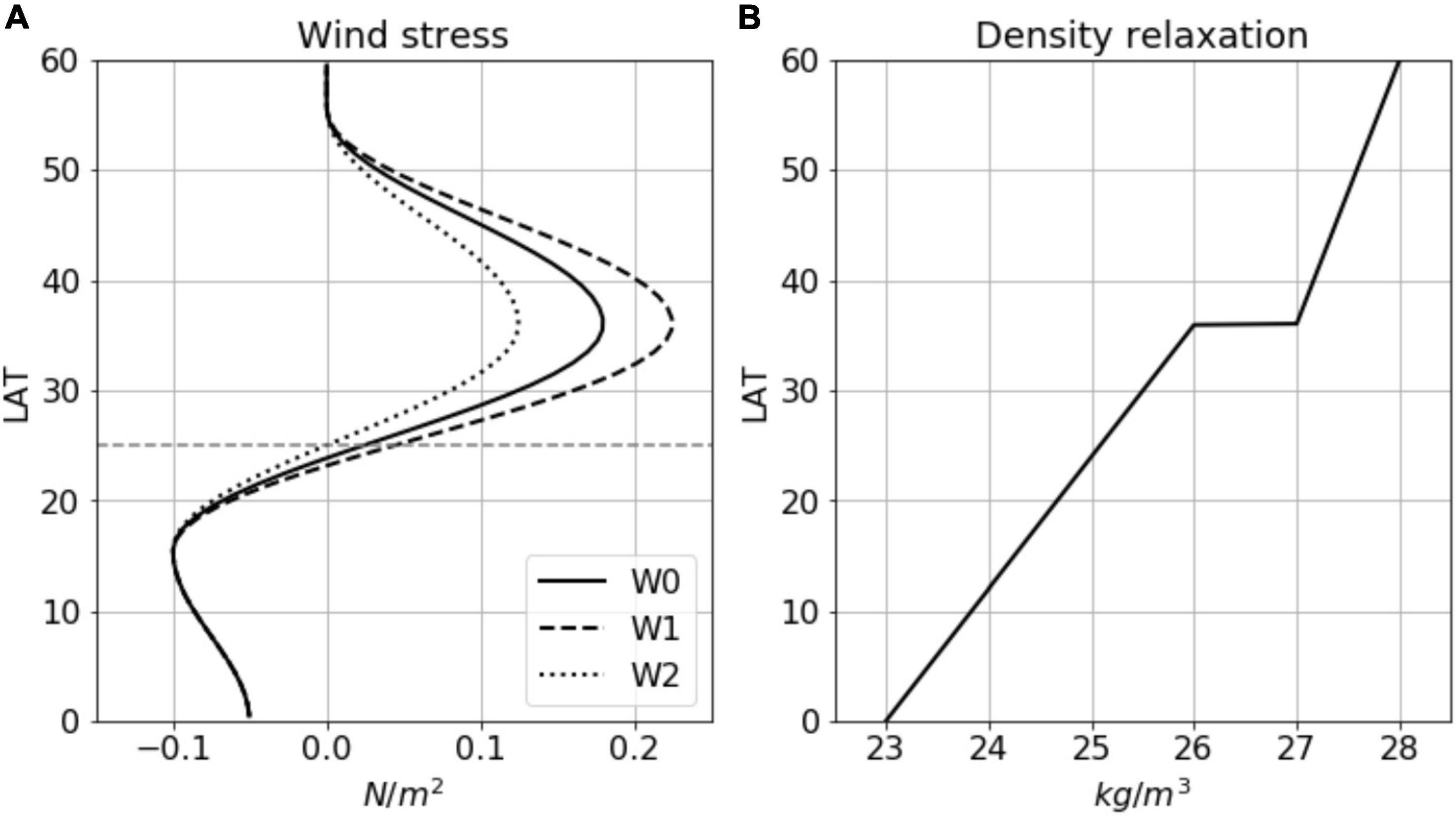
Figure 1. Surface forcing of the model. (A) Zonal wind profiles. The solid line (W0) is the zonal wind used in experiments D1, D3.2, D10, and D32. The other two lines are the zonal wind used in sensitivity experiments. The gray dashed line means the latitude. (B) Restoring sea surface density. A density “jump” at 36°N is specified to simulate the strong convective overturning poleward of the subtropical front, as in the real ocean.
The restoration time scale for the surface density is taken to be 40 days (for the top layer of 10 m), which implies a restoration coefficient γ = 0.25 m day−1. A density “jump” at 36°N (Figure 1B) aligning with the maximum eastward wind is imposed to simulate the deep convection just poleward of the subtropical front (McCartney and Talley, 1982). To simplify the model configuration, only constant wind and buoyancy forcing are applied in this study.
To assess the role of eddies, four horizontal grid spacings of 1°, 1/3.2°, 1/10°, and 1/32° are used, which will be referred to as coarse-grid, eddy-permitting, eddy-resolving, and fine-grid, and designated by D1, D3.2, D10, and D32 experiments (“D” for “Degree”), respectively. To our knowledge, 1/10° grid has often been referred to as “high resolution” in the past two decades until more “super-high resolution” numerical calculations are carried out recently, such as 1/48° by Rocha et al. (2016), 1/54° by Lévy et al. (2010), and 1/64° by Hurlburt and Hogan (2000). These studies however are concerned mainly with simulating the eddies while our aim is to assess the eddy effect on the mean circulation, which turns out to be adequately addressed by the range of the grid spacings we have selected.
All experiments with varying resolutions and wind profiles are summarized in Table 1. Experiments D1, D3.2, D10, and D32 are driven by the same wind profile (W0) and the experiments using wind profiles W1 and W2 are tagged as D1W1 and D1W2, D10W1 and D10W2 correspondingly. They are compared with D1 and D10 to examine the model sensitivity to the wind forcing. The model integrations are carried out in two stages of spin-up and experimental run. First, the 1° model is initialized with vertical stratification derived from the domain-averaged temperature in the North Atlantic based on the World Ocean Atlas 2013, and integrated for 250 years to reach a quasi-equilibrium. From this point on, all experiments are run for another 50 years. Figure 2 shows time series of domain-averaged kinetic energy above a depth of 1,000 m for all experiments, which suggests that it is sufficient for 50 years to equilibrate the upper ocean circulation that we focus. A time-average over the last 20 years is used for the following analysis.
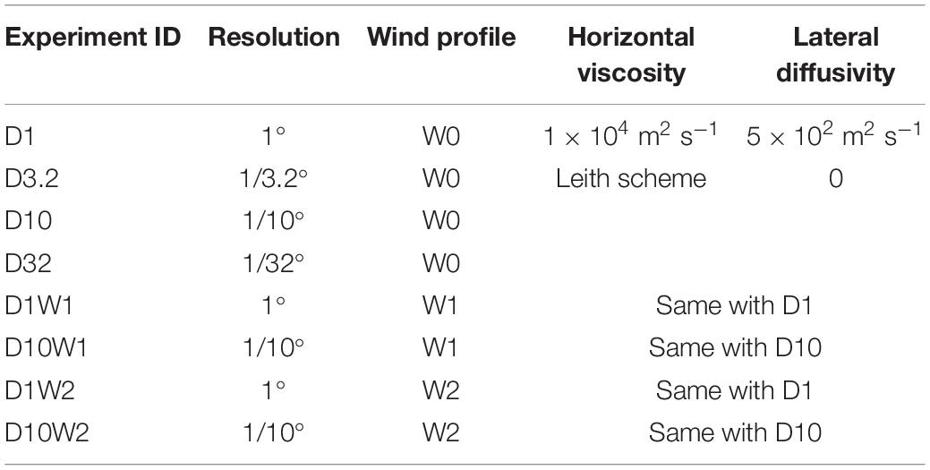
Table 1. Experiment designation.
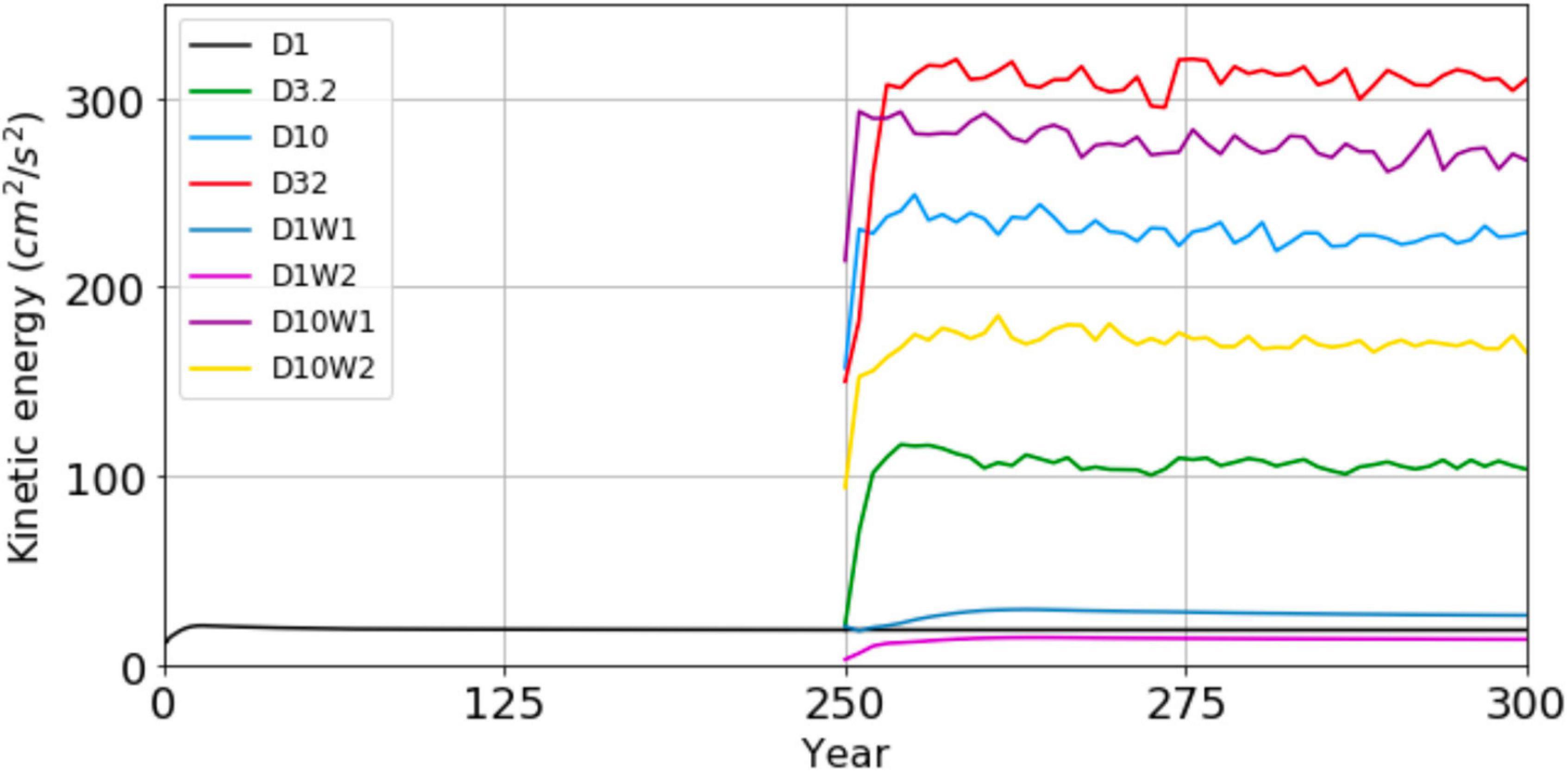
Figure 2. Time series of domain-averaged kinetic energy above a depth of 1,000 m for all experiments.
For the 1° case, horizontal momentum dissipation is provided by a Laplacian viscosity (Ah = 1 × 10⁴ m2 s−1), and the lateral heat diffusivity Kh is set to 5 × 10² m2 s−1. For the other cases, the biharmonic viscosity is calculated according to the velocity gradient based on the modified Leith scheme (Fox-Kemper and Menemenlis, 2008), and the lateral heat diffusivity is set to 0. For all cases, the vertical viscosity Av is set to 1 × 10⁻⁴ m2 s−1, and the diapycnal diffusivity Kv is 1 × 10⁻⁷ m2 s−1. Unless otherwise mentioned, the viscosity and diffusivity both take the Laplacian form. Further details of the physical parameters used in the model are available at https://github.com/liutongya/PV_circulation.
It is expected that higher resolution models contain more energetic eddies and simulate the finer structure of the upper ocean (Bryan et al., 2007; Lévy et al., 2010; Chassignet and Xu, 2017). Figure 3 shows random snapshots of the sea surface temperature in D1, D3.2, D10, and D32. It is seen that the coarse-grid experiment (D1) cannot resolve mesoscale eddies, and the eddy-permitting experiment (D3.2) can reveal the temperature disturbance induced by large-size eddies. In the eddy-resolving experiment (D10), the basin is full of mesoscale eddies, especially in the subtropical gyre (between 10°N and 40°N). The fine-grid experiment (D32), in addition to mesoscale eddies, also partially resolves submesoscale and filamentary structures induced by nonlinear processes. The stretching and folding of filaments is known to be particularly effective in homogenizing the PV over the macroscopic scale (Brown and Smith, 1991; Beron-Vera and Olascoaga, 2009). Figure 4 shows zonally-averaged EKE at the surface. In this study, the time-mean EKE is defined as , where u′ and v′ are the time-varying components of the surface velocity. The EKE of D1 is near zero, so the mean is numerically well approximated by the instantaneous field because the fluctuations are quite small. For the other experiments, the EKE varies with the latitude and all peaks just south of the subtropical front in all cases. In D10, the maximum EKE exceeds 1, 000 cm2 s−2 and in D32, it is further doubled to 2, 000 cm2 s−2. We shall next diagnose the roles of eddies in the structure of the upper-ocean circulation. Note that eddies in this study are defined as deviations from the time-mean background flow.
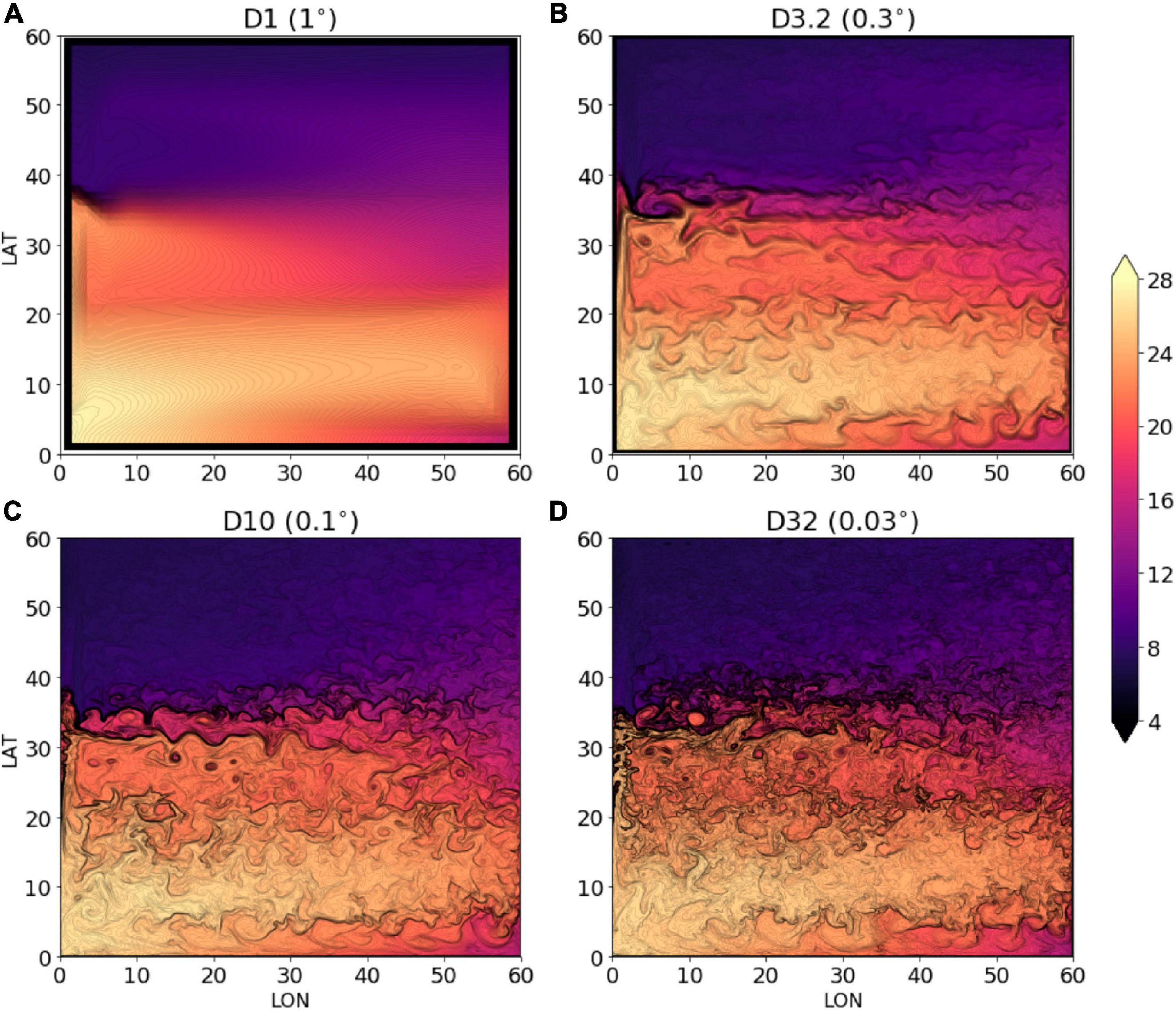
Figure 3. Snapshots of sea surface temperature (in °C) in experiments (A) D1, (B) D3.2, (C) D10, and (D) D32. Black contours of 0.1°C interval are plotted to delineate the eddies.
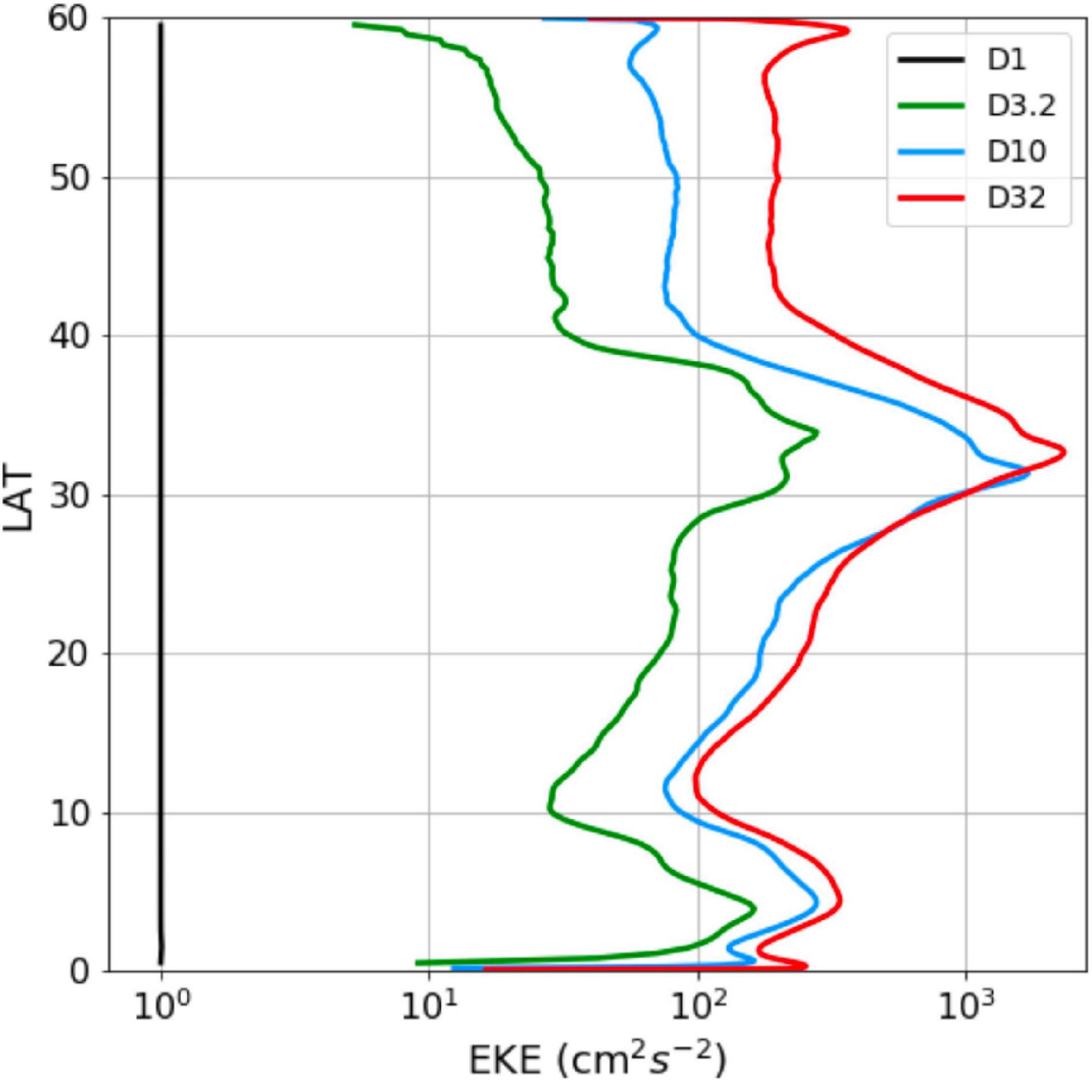
Figure 4. Zonal-averaged EKE (in cm2 s−2) at the surface from the four experiments.
Figure 5 shows the mean sea surface height (SSH) from the four experiments. In all cases, the zonal wind stress drives a classical double gyre (subtropical and subpolar) circulation pattern with a strong eastward current between the two gyres resembling the Gulf Stream extension (GSE). On account of hydrostatic balance, the SSH is proportional to the main thermocline depth (Rebert et al., 1985; Huang, 2015). Here, we use the SSH field to reflect the pattern of the main thermocline structure. According to the Sverdrup dynamics, the thermocline depth should respond to the Ekman pumping (Welander, 1968), which is downward (upward) in the subtropical (subpolar) region. In D1, the latitude of the maximum thermocline depth roughly coincides with that of the maximum wind stress curl (about 25°N), as expected from the Sverdrup dynamics. The qualitative changes in the circulation pattern with increasing resolution are significant. Compared with D1, the maximum depths of the thermocline in D10 and D32 are seen to move northward from the subtropical interior (about 25°N) to just south of the subtropical front (about 30°N). Moreover, their SSH patterns are quite comparable to the mean dynamic topography observed in the North Pacific or the North Atlantic (see Figure 3 in Rio et al., 2011).
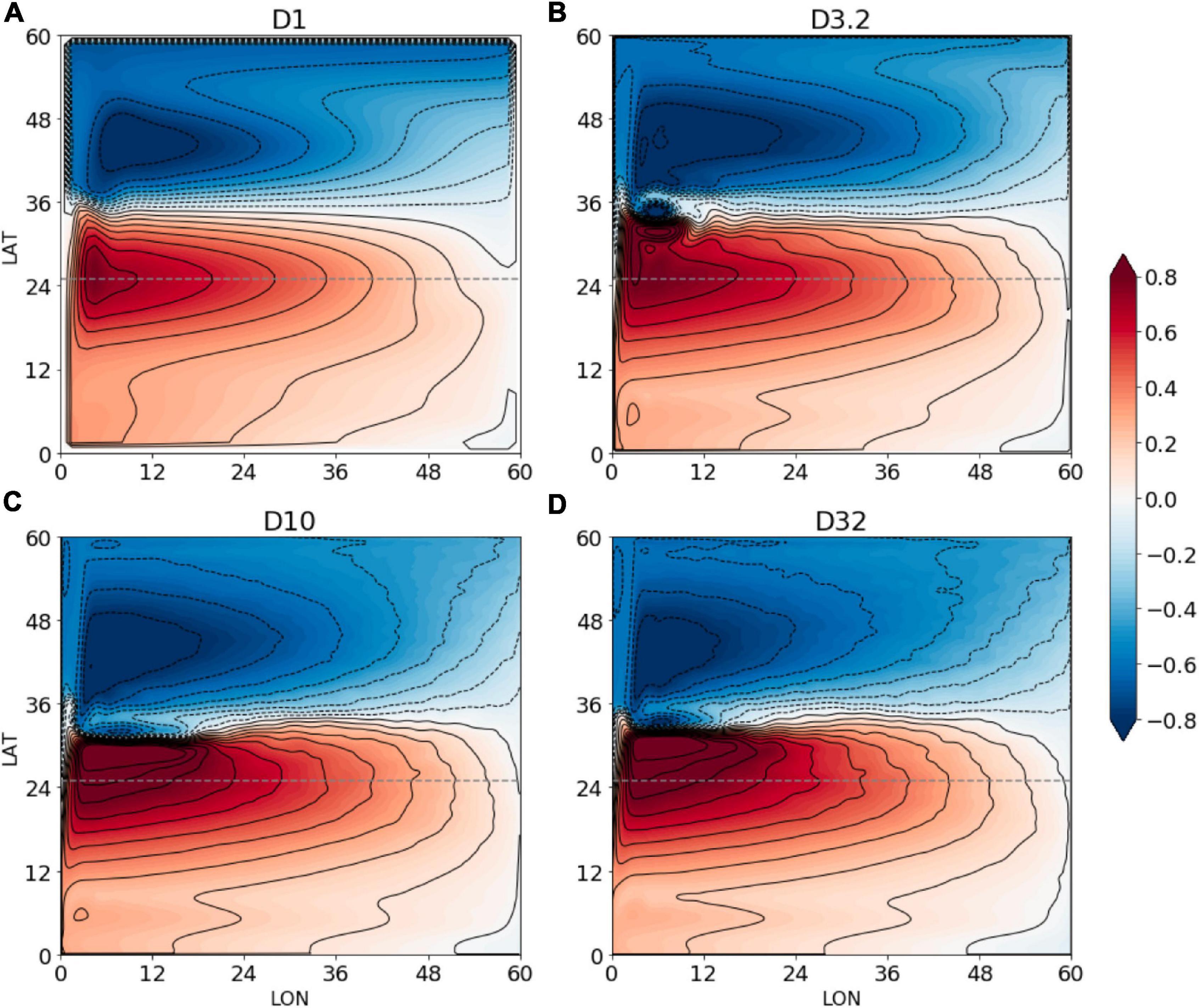
Figure 5. Time-averaged SSH (in meters) from the four experiments. The contour interval is 0.1 m. The dashed line marks the latitude of the maximum wind stress curl. (A–D) Correspond to experiments D1, D3.2, D10, and D32, respectively.
To understand the eddy effect within the subtropical gyre, Figure 6 shows the spatial distribution of the EKE in D32. It is seen that the surface EKE is greater than 100 cm2 s−2 throughout the subtropical gyre, and exceeds 1, 600 cm2 s−2 near the subtropical front, which is supported by the estimate in the North Atlantic based on surface drifters (Maximenko et al., 2013). In the vertical, the EKE is greater than 100 cm2 s−2 above 400 m in the subtropical interior and above 800 m just south of the subtropical front. Compared with high-resolution simulations by Lévy et al. (2010, their Figure 4) and Chassignet and Xu (2017, their Figure 4), the EKE distribution from our model shows the similar pattern, which represents that our model is capable to well resolve the active eddy activities.
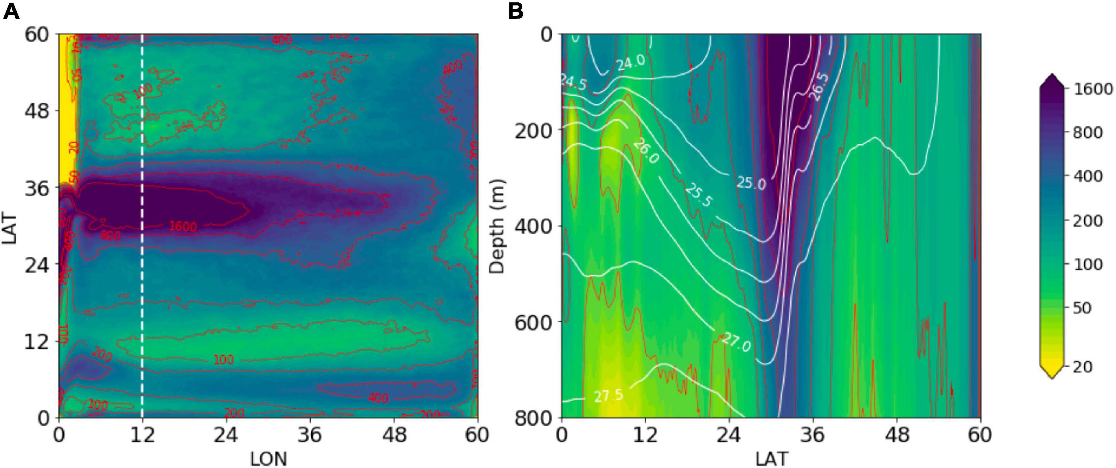
Figure 6. Spatial distribution of the EKE (in cm2 s−2) in D32. (A) The surface map. (B) The meridional section along 12°E, overlaid by the density field (white contours).
Figure 7 shows isopycnals and zonal velocity along the 12°E meridian with the isopycnal 26.5 (green line) marking the main thermocline. This isopycnal has been selected as the main thermocline because it is close to the maximum vertical temperature gradient in the subtropical region and it outcrops near the latitude where the wind stress curl is zero. Our model has generated the main zonal flows observed in the subtropics (Qiu and Chen, 2010), such as the westward North Equatorial Current and the eastward GSE (from 10°N to 30°N in Figure 7). Model solutions show significant variation in the strength and width of these currents with increasing grid resolution. In D1, the North Equatorial Current is comparable with the GSE in both width and speed, which is at odds with observations. In D3.2, the GSE becomes much more concentrated in a narrow latitudinal band and moves faster than that in D1. This trend continues for D10 and D32 when the GSE reaches speed exceeding 1 m s−1, much closer to its observed speed (Hall, 1989). And the GSE with velocity exceeding 0.5 m s−1 can extend to about 20°E in D10 and D32, which agrees with the simulation of Lévy et al. (2010, their Figure 5). Satellite observations show that the length of GSE can extend further eastward (Chassignet and Xu, 2017) than our idealized model, reaching about 30° of longitude. This difference might be attributed to the idealized surface forcing and the absence of realistic topography.
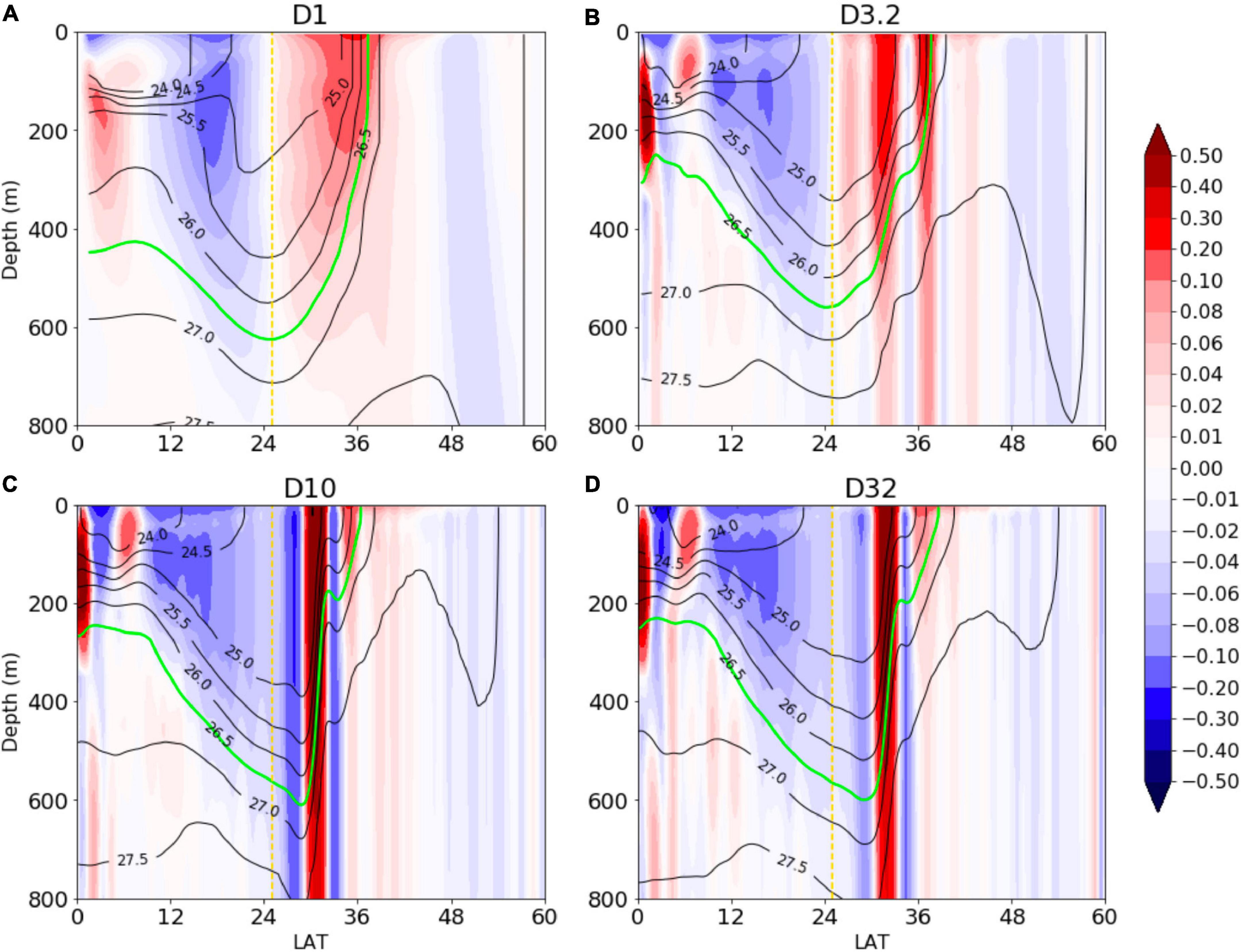
Figure 7. Meridional sections of zonal velocity (colored, in m s−1) and density (contoured) along 12°E, with the green line marking the main thermocline. The yellow dashed line represents the latitude of the maximum wind stress curl. (A–D) Correspond to experiments D1, D3.2, D10, and D32, respectively.
As discussed in connection with Figure 5, the increasing resolution also has profound effects on the thermocline shape. In D10 and D32, it is seen that the thermocline deepens linearly with the latitude from 10°N to about 30°N and then rises sharply across the GSE. This structure cannot be captured by Sverdrup dynamics and the coarse-grid experiment. That the thermocline in the subtropical gyre deepens linearly with the latitude is first noticed by Stommel (1965) from which he surmised that the columnar PV above the main thermocline should be homogenized. Previous numerical models have demonstrated that the GSE is narrower and stronger in the eddy-resolving runs, but some low-resolution numerical models fail to reproduce the above thermocline structure because they are insufficient to fully capture the effect of strong eddy mixing (e.g., Henning and Vallis, 2004).
Having described the circulation structure for four experiments, here we focus on the core issue of this study by diagnosing the PV balance. The key question is how the eddy mixing affects the PV distribution and upper-ocean circulation in the subtropics. For the columnar motion above the main thermocline, the macroscopic PV balance is described as (Young, 1987; Ou, 2013):
where
is the columnar PV, with f, the Coriolis parameter on the sphericity, h, the main thermocline depth, , the horizontal layer-averaged velocity, , the wind stress, ρ0, the reference ocean density, κ is the eddy diffusivity, and is the unit vector. Equation 3 states that the PV input by wind (the RHS) is balanced by the mean advection (the first term) and eddy mixing (the second term). If the eddy mixing and the relative vorticity are neglected, the equation is reduced to the generalized Sverdrup balance above the main thermocline (Welander, 1968),
However, Sverdrup balance would be nullified if the eddy mixing dominates the mean advection. In the asymptotic limit of large eddy diffusivity, Eq. 3 implies that the PV would be a harmonic function. Subjected to the Neumann condition of vanishing normal PV gradient (since the normal flux is finite to balance the wind input), the PV is then homogenized (Ou, 2021).
Maps of isopycnal PV calculated from hydrographic data show a high degree of homogenization in the subtropical interior (Holland et al., 1984; Keffer, 1985; Talley, 1988), and the meridional section shows that isopycnal PV isolines are nearly parallel to the isopycnals between the tropics and the subtropical front (McDowell et al., 1982). Computationally, primitive-equation models (Cox, 1985; Nakamura and Kagimoto, 2006) show the PV homogenization along the isopycnals away from the surface forcing. Our experiment D3.2 has reproduced the results of Cox (1985) that eddy mixing is quite effective in homogenizing isopycnal PV in the interior, and the experiment D32 shows even higher degree of the homogenization of the isopycnal PV (not shown). In this study, however, we focus on the columnar PV, rather than isopycnal PV, which can be directly translated to the subtropical gyre above the main thermocline—the primary feature of the general ocean circulation that we are concerned with.
From the thermocline depth, we calculate the columnar PV based on Eq. 4, which is shown in Figure 8. It is seen that the PV distribution in D1 is as expected from Sverdrup balance with strong meridional gradients in the subtropical interior to reflect the PV input by the wind stress curl. In D3.2, the weak eddy mixing only marginally modifies the PV distribution between about 10°N and 25°N. In D10 and D32, however, the PV is seen to be significantly homogenized in the subtropical interior (from about 10°E to 40°E) with its gradient expelled to the tropics, the western boundary and the subtropical front, which agrees with the observational analysis of Stommel (1965) and Toole et al. (1990). Our model thus captures the effect of the eddy mixing of PV to render gyre-wide homogenization of the macroscopic PV. It is worth noting that although the EKE has doubled from D10 to D32, the homogenized area does not expand significantly because the area already covers most of the subtropical gyre domain. Since the subtropical gyre constitutes a primary feature of the upper ocean circulation, the PV homogenization, which spans the gyre, may thus provide a useful dynamical principle of the general ocean circulation.
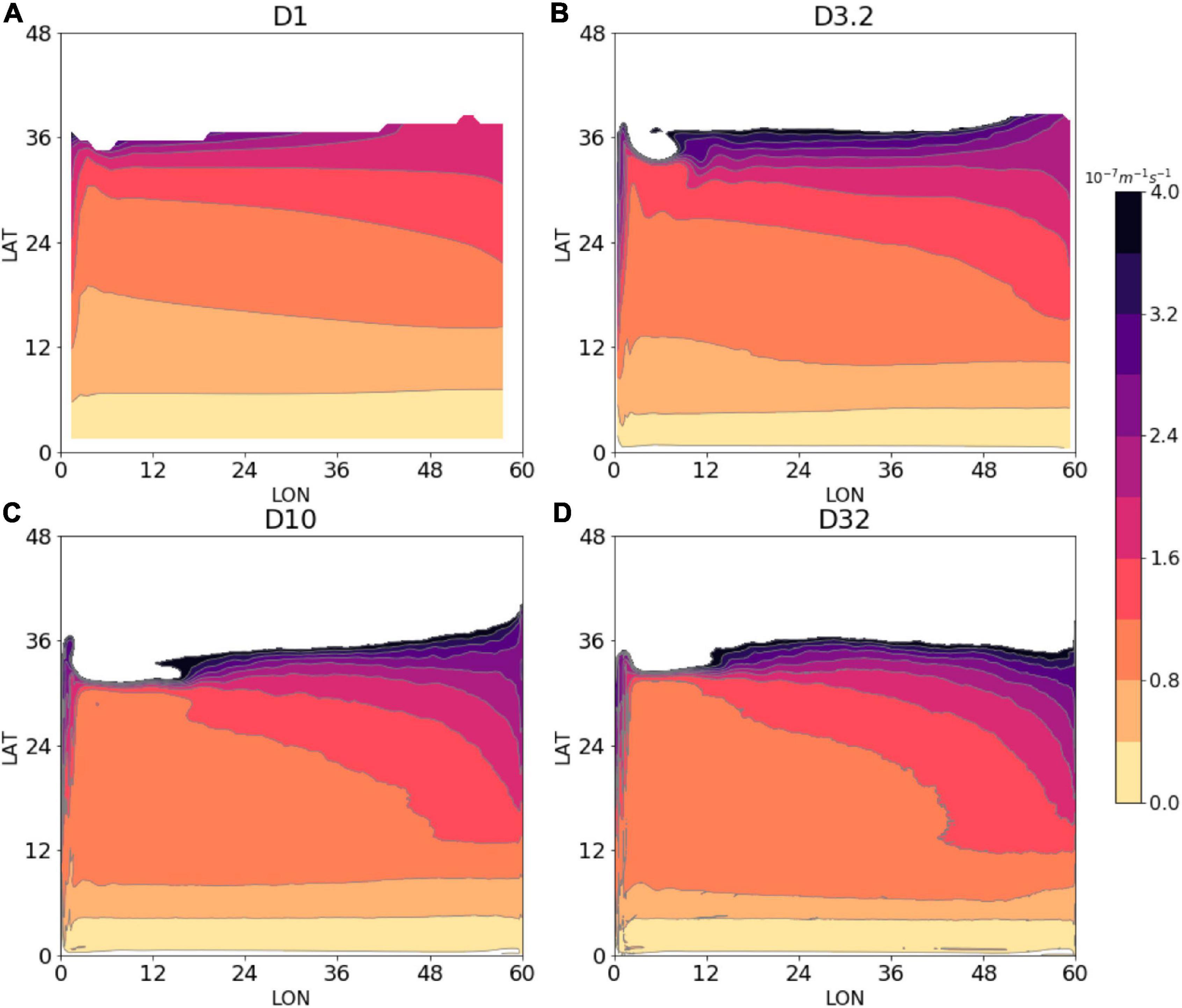
Figure 8. Time-averaged columnar PV (in 10−7 m−1 s−1) calculated from the thermocline depth. Note that the white part represents the region north of where the main thermocline outcrops. (A–D) Correspond to experiments D1, D3.2, D10, and D32, respectively.
As a step in his formulation of the climate theory, Ou (2018) examines the different fields interactive with the thermohaline circulation (THC), which is a generalized meridional overturning cell that includes random eddy exchange across the subtropical front. The strength of the THC (K) is defined as the zonal-averaged mass exchange rate between the warm and the subpolar waters, which has the unit of the volume transport divided by the basin width (hence, m2 s−1). The THC would moderate their heat and PV differences between the two regions. Then K can be diagnosed from the buoyancy balance of the mode water
where ρ* is the restoring surface density, γ is the restoration coefficient, φ is the outcrop latitude, and Δρ is the density difference between the warm layer and the subpolar region. In the 1/32° run, the buoyancy gained by the warm layer south of the subtropical front (the LHS) is about 4.8 kg m−1 s−1, and Δρ has a range of 0.75 ∼ 1 kg m3, so K is calculated to be 4.8 ∼ 6.4 m2 s−1. Then the basin-integrated meridional overturning cell is estimated to be 28.8 ∼ 38.8 Sv, which is close to the previous estimate in the North Atlantic (Cessi, 2019).
As the THC also transports the PV across the subtropical front, its diagnosis allows us to estimate the homogenized PV from the PV budget of the warm layer. The PV balance in Eq. 3 indicates that the source of the PV is the net wind curl Δτ over the warm water, and the primary sink is the eddy flux across the subtropical front when the PV is homogenized (Harrison, 1981; Ou, 2013). Then the PV budget in the subtropical gyre is a balance between the input from winds and the meridional PV flux by eddy mixing from the homogenized warm layer to the subpolar region (see Figure 1 in Ou, 2013), which is described as
where Q is the homogenized PV we seek to determine, f0 the Coriolis parameter at the subtropical front (30°N), Hm ≈ 200 m is the relevant depth where the thermocline intersects the subtropical front, and Δτ = 0.28 N m−2 is the zonal wind range across the subtropics. We assume that the subtropical front is quite narrow, then approximately represents the PV just north of the subtropical front. Rearranging Eq. 7, we obtain
where
thus calculating the homogenized PV. In addition, let H denotes the maximum thermocline depth just south of the narrow GSE, it is then given by
Based on K estimated earlier, λ has the range 0.2 ∼ 0.4. So H has the range 500 ∼ 1000 m, and Q = 0.73 ∼ 1.45 × 10⁻⁷ m−1 s−1 (shown by the gray region in Figure 9). The PV value given here is a plausible range, not an exact value, because we diagnose it based on the asymptotic limit of fully homogenized PV, and then there are uncertainties in other parameters in the calculation of the PV values, including the density difference across the front. In Figure 9, we plot the columnar PV averaged between 10°E and 40°E to examine its variation with the latitude in the subtropical gyre. We have considered the latitude band between 10°N marking the southern extent of the subtropics and the outcrop latitude where the main thermocline reaches the subtropical front (the northern edge of the GSE). Instead of aligning with the maximum of the westerly wind stress, the outcrop latitude is shifted southward about 5° from D1 to D32, which can be attributed to nonlinear effects due to the mesoscale turbulence (Lévy et al., 2010). In D1, the PV increases strongly with the latitude, spanning a range of about 1.7 × 10⁻⁷ m−1 s−1 in the subtropics. This range is progressively reduced by increasing resolution, and in D32, the PV range spans only about 0.4 × 10⁻⁷ m−1 s−1, or only approximately 25% of the non-eddy case. This provides a quantitative statement of the PV homogenization by the eddy mixing. In support of the range of the homogenized PV diagnosed earlier, the PV profile of D32 falls within this range (shaded).
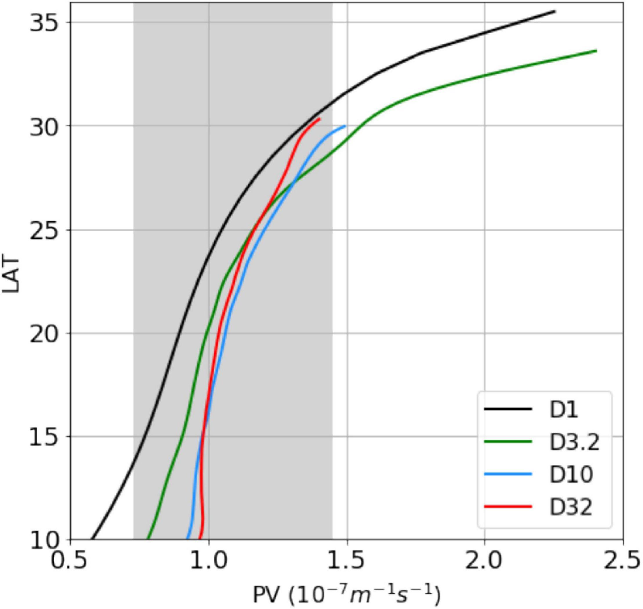
Figure 9. The columnar PV, zonally averaged between 10°E and 40°E, and plotted against latitude spanning the subtropics. These four lines terminate at the outcrop latitude, and the gray region indicates the range of the homogenized PV calculated from the PV budget.
Equation 3 indicates that the large-scale circulation of the upper ocean is primarily modulated by two regimes: PV mixing versus Sverdrup balance. Having discussed the role of eddy mixing in the PV distribution, now we focus on the relative contributions of these two regimes to the subtropical circulation.
As a zeroth-order theory of wind-driven motion, Sverdrup balance is based on laminar dynamics hence is not expected to apply where eddy mixing of PV is strong. The two-layer quasi-geostrophic model of Holland and Rhines (1980) has examined the applicability of the Sverdrup dynamics in a two-gyre basin containing energetic eddies and showed that Sverdrup balance holds only over a small fraction of the basin (his Figure 3). Observational analysis incorporating Argo floats (Gray and Riser, 2014) suggests that the Sverdrup dynamics may account for the meridional transports in the tropics and subtropics, but fails in higher latitudes and boundary regions due to the effects of barotropic flow, nonlinear dynamical processes, and topography. Few studies have examined the effect of the eddy mixing on the Sverdrup relationship in the interior, a significant gap we seek to fill in this study.
To quantify the effects of eddy mixing on Sverdrup balance, we define from Eq. 5 the deviation from the classical Sverdrup relationship
We then calculate the ratio
which can be interpreted as the percentage within which Sverdrup balance holds. The closer to zero is, to a greater degree the Sverdrup relationship holds. Following Holland and Rhines (1980), we set ε < 0.2 as the spatial domain where Sverdrup balance approximately holds, which we shall refer for convenience as the Sverdrup domain. This domain is shown by shaded regions in Figure 10, which is overlaid with the thermocline depth in red contours. For the coarse-grid experiment (D1), the Sverdrup domain covers the whole subtropics except near the western boundary layer where the inertial-viscous balance dominates (Munk, 1950; Pedlosky, 1987). For the eddy-permitting experiment (D3.2), the Sverdrup domain has shrunk considerably to limited regions in the interior and near the eastern boundary. This trend continues for the eddy-resolving experiment (D10) with much enhanced eddy mixing, and for the fine-grid experiment (D32), stronger eddy mixing induced by resolved filaments should further reduce the Sverdrup domain to a few isolated patches. Quantitatively, from D1 to D32, the Sverdrup domain in the subtropics has shrunk by more than 60%.
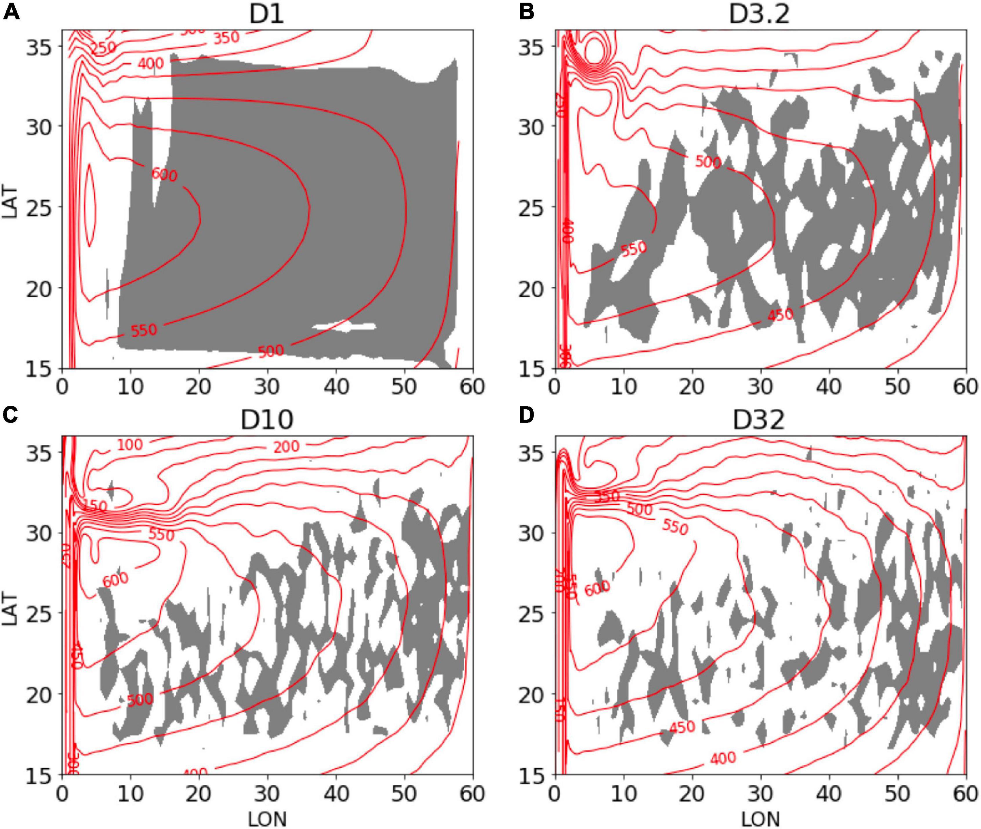
Figure 10. Sverdrup domain (shaded) with the depth of the 26.5 isopycnal overlaid in red contours. The Sverdrup domain is defined by (Eq. 12) being smaller than 0.2. (A–D) Correspond to experiments D1, D3.2, D10, and D32, respectively.
To provide another quantitative statement of the PV-mixing effect, zonally averaged values of ε in the western boundary (from 0°E to 10°E), interior (from 10°E to 40°E), and eastern boundary (from 40°E to 60°E) regions of the subtropical gyre are calculated (Figure 11). In the western boundary region, the values from the four experiments are all high due to the strong nonlinear advection and bottom pressure torque (Liu et al., 2020). In the interior region, from D1 to D32, the differences induced by the eddies are obvious and the averaged increases from about 0.1 to 0.4, which means the eddy mixing contributes about 30% to the vorticity balance. In the eastern boundary region, the eddy effects are also significant in shaping the boundary current (Bire and Wolfe, 2018) but would not cause PV homogenization. Note that the PV mixing regime is only applied in the interior region (Ou, 2021) where the PV homogenization exists. Although the proportion of the eddy mixing in the PV balance is not dominantly large, our results suggest that the eddy effects on PV distributions cannot be neglected in the quieter subtropical interior.
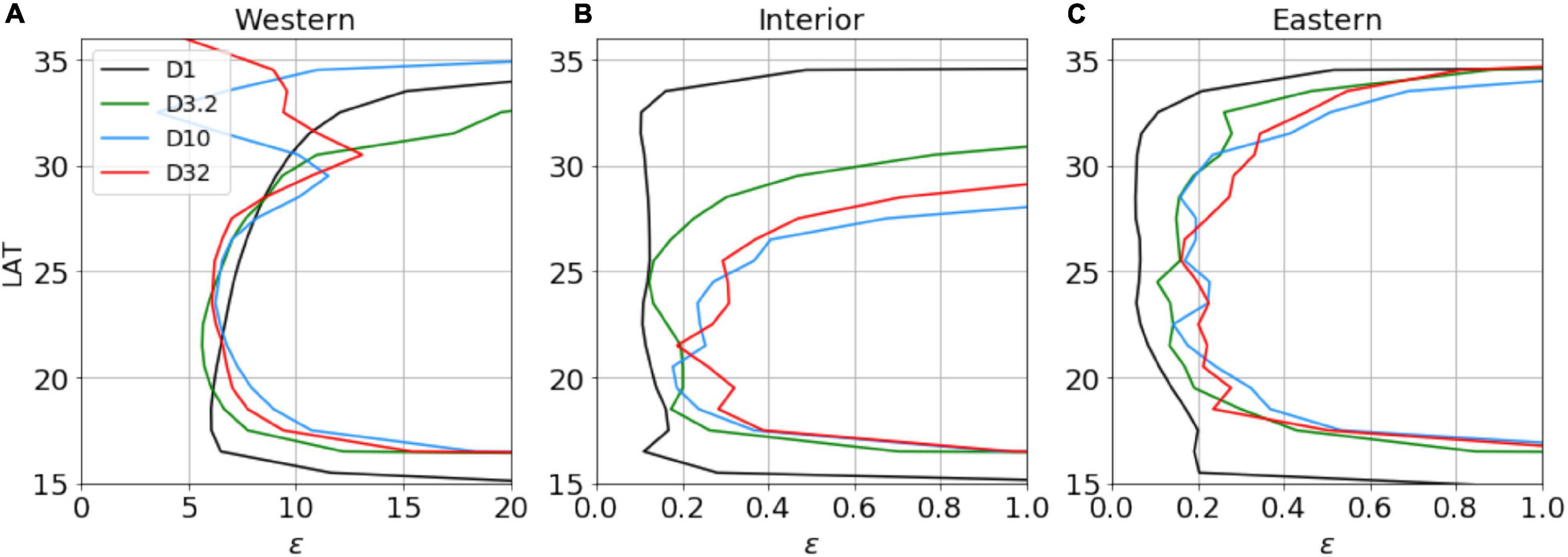
Figure 11. Zonally averaged values of ε (Eq. 12) in the (A) western boundary (from 0°E to 10°E), (B) interior (from 10°E to 40°E), and (C) eastern boundary (from 40°E to 60°E) regions of the subtropical gyre.
Here, we provide a rough estimate of the basin-wide eddy diffusivity in D32 from the vorticity equation. Since the mixing term accounts for about 30% in the PV balance, applying the scale estimates based on Eq. 3, we can get the magnitude of the eddy diffusivity
where, h ≈ 500 m is the thermocline depth, L ≈ 1500 km denotes the meridional range of the subtropical gyre. Then, the eddy diffusivity in D32 is about 1 × 10⁴ m2 s−1, indicating that the eddy activity would lead to a strong mixing regime to homogenize PV, but D1 is very far from that regime because the resolution is insufficient to resolve eddies and no eddy parameterization scheme is employed. In this study, the eddy diffusivity is a proxy of the stirring induced by mesoscale eddies and sub-mesoscale structures, including not only the local eddy mixing (Groeskamp et al., 2020), but also chaotic stirring (Pierrehumbert, 1991; Beron-Vera and Olascoaga, 2009) and nonlocal eddy transports that are difficult to be represented by a local diffusivity.
Since the general ocean circulation has largely converged from 1/10° to 1/32° and given the inordinate computational resources required of 1/32° runs, it suffices to use the 1/10° experiment to examine the solution sensitivity to the varying wind profile. In Figure 12, we compare the thermocline depth from the coarse-grid (D1) and eddy-resolving (D10) runs with the analytical solutions from the Sverdrup and PV mixing regimes. For the numerical solutions, three wind profiles are used to assess their sensitivity. In Figure 12A, the analytical Sverdrup solution is calculated from (Huang, 2010),
where the thermocline depth at the eastern boundary he is set to 400m, reduced gravity g′ = 0.02 m s−2, Lx is the distance from the eastern boundary. It is seen that the coarse-grid solutions (solid lines) indeed trace closely the analytical curve to fall within the Sverdrup regime (blue dashed line). The latitude of the maximum thermocline depth aligns roughly with that of the maximum wind stress curl and the numerical solutions shift with the different winds, both as predicted from Eq. 14.
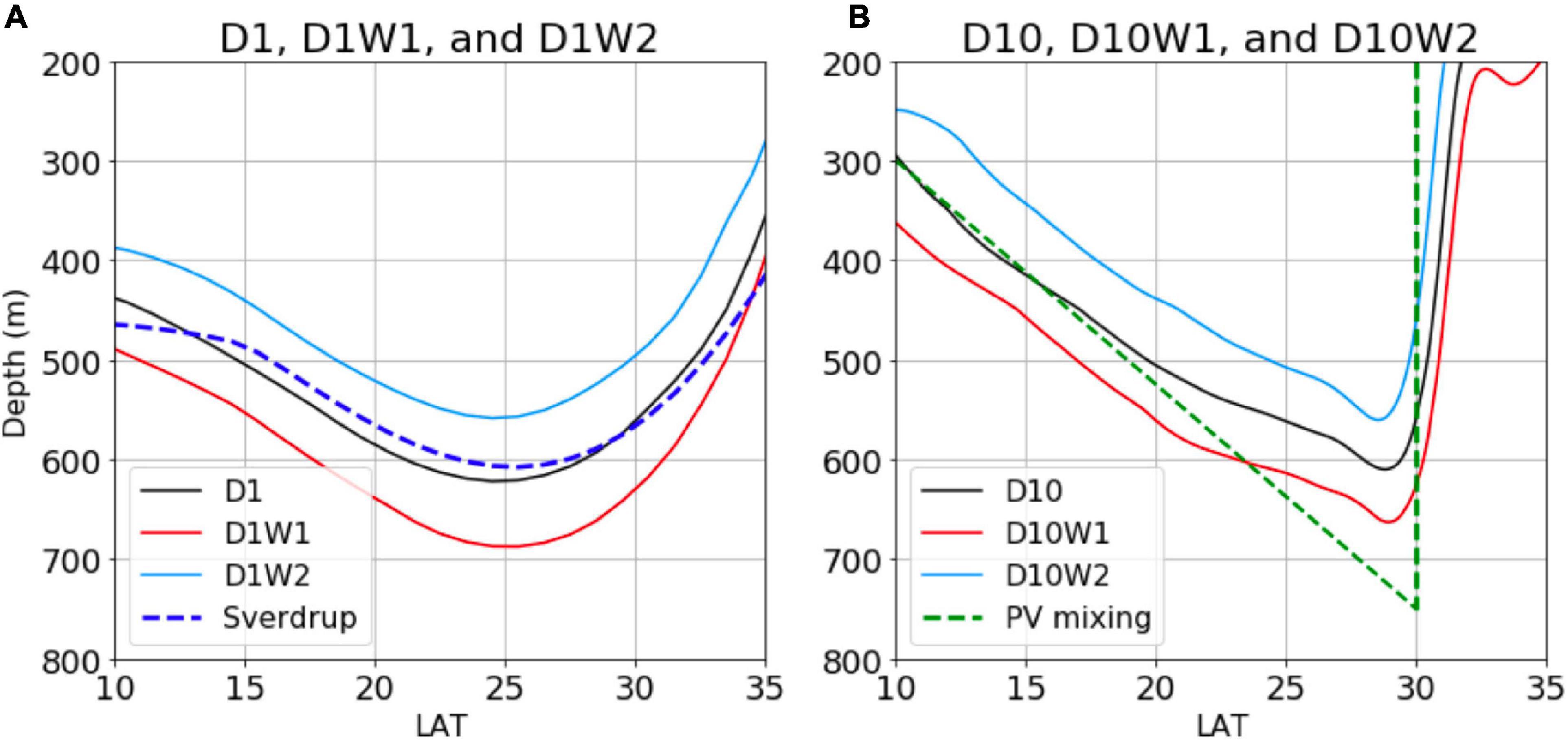
Figure 12. Comparison of the thermocline depth along 12°E between the numerical and analytical solutions. (A) The coarse-grid (1°) numerical solutions using different wind profiles (solid lines); (B) same as (A) but the numerical solutions are from eddy-resolving (1/10°) calculations. Analytical solutions for two theories based on reference cases (D1 and D10) are marked by dashed lines.
In Figure 12B, the analytical solution of the homogenized PV with its medium value (as estimated in section “Potential Vorticity Homogenization in the Subtropical Gyre”) is used here for the theoretical curve. Since the relative vorticity is negligible in the subtropical interior, the homogenized PV implies that the thermocline deepens linearly with the latitude before it shoals abruptly across the subtropical front. Compared with the Sverdrup solution, the thermocline patterns in eddy-resolving solutions are closer to the analytical solution based on PV homogenization. Varying wind stress also shifts the numerical solution in accordance with the theoretical prediction (Eq. 10). Our results suggest that the maximum thermocline depth is determined by wind stress curl, but the thermocline structure is modulated by eddy mixing. In addition, from 20°N to 30°N, the thermocline structure is not perfectly captured by the PV mixing regime. The reason might be that completely homogenized PV in the subtropical gyre is an idealized condition, which is difficult to achieve in the model and real ocean. Additionally, the inertial term might also affect the gyre pattern in the recirculation region (Cessi et al., 1987). While there remains some difference between the numerical and analytical solutions, it is patently clear that the PV mixing regime provides a brief and reasonable explanation of the eddy-resolving solutions.
Classic wind-driven theories based on Sverdrup balance have difficulties in explaining some features of the observed circulation. This is because these theories mostly do not consider the eddy mixing, which tends to homogenize the macroscopic PV to break Sverdrup balance. In its application to the atmosphere, Ou (2013) shows that the PV homogenization may reproduce the prevailing wind, which thus may serve as a governing principle of the general atmospheric circulation. The present study aims to assess the role of PV mixing by eddies in the general ocean circulation. Although PV homogenization in the subtropical ocean has been discerned by observations and numerical models (McDowell et al., 1982; Rhines and Young, 1982; Cox, 1985), we attempt to provide a quantitative assessment of the regime from numerical experiments.
We consider an idealized ocean basin in the Northern Hemisphere and conduct a series of numerical experiments using the MITgcm with varying horizontal grid spacings and wind forcing. To assess the effect of eddy mixing on the upper-ocean circulation, numerical calculations using four grid spacings of 1°, 1/3.2°, 1/10°, and 1/32° are carried out. With increasing resolution from the coarse-grid to the eddy-resolving runs, the teeming eddies emerge to qualitatively alter the macroscopic circulation. In the coarse-grid (1°) case, the structure of the thermocline is as expected from the Sverdrup dynamics with its maximum depth located in the subtropical interior. With increasing resolution, this maximum depth is seen to migrate toward the subtropical front. Particularly, the eddy-resolving (1/10°) and fine-grid (1/32°) experiments show a thermocline that deepens linearly with latitude until it shoals abruptly across the subtropical front, which is close to its observed structure (Qiu and Chen, 2010).
Although several studies (Cox, 1985; Henning and Vallis, 2004; Lévy et al., 2010) have discerned the changing subtropical circulation when eddies are resolved, our principal innovation is to provide a quantitative assessment of the eddy-mixing regime by comparing the numerical and analytical solutions. Our numerical solutions show that eddy mixing is quite effective in homogenizing the PV in the subtropical gyre, reducing its meridional range by about 75% when the grid spacing decreases from 1° to 1/32°. We also find that the Sverdrup domain is relegated to isolated patches in the fine-grid (1/32°) experiments, with its area reduced by about 60% from the coarse-grid runs. In addition, sensitivity experiments show that the maximum thermocline depth is modulated by wind stress curl, but the thermocline structure is reshaped by eddy mixing. In eddy-resolving cases, the thermocline structure can be mostly captured by the homogenized PV regime, which provides a reasonable explanation of the observed subtropical gyre.
It is necessary to point out several limitations of the PV mixing regime. Simulations based on a three-layer quasi-geostrophic model show that the PV homogenization typically occurs in the subtropical gyre (Maddison et al., 2015), supporting our results here. But there are obvious PV gradients in the top layer due to the strong forcing and dissipation (corresponding to PV sources and sinks), which is also captured by observations that the region with homogenized PV is very limited along the isopycnals near the surface (McDowell et al., 1982; Talley, 1988). To simplify the question and compare with the classic Sverdrup theory, we only consider the columnar PV above the main thermocline and neglect the vertical structure of the upper circulation. Moreover, the completed PV homogenization in the subtropical gyre is obtained in the hypothesis of infinitely strong eddy mixing (derived from Eq. 3). Observations suggest that the strength of eddy mixing has obvious spatial patterns and limited values (Abernathey and Marshall, 2013), and the homogenized PV is not observed in the boundary regions of the subtropical gyre (Talley, 1988). This is the gap between the PV mixing theory and the real ocean.
It should be noted that this study is not intended to replace these theories based on the Sverdrup dynamics, but merely to examine the novel circulation theory by Ou (2013, 2021) and present a different perspective to explain the complicated general ocean circulation via numerical simulations. In spite of these limitations of the PV mixing regime, guiding principles from this study remain clear: Sverdrup balance is an effective framework of the wind-driven circulation, but it is unable to fully describe the structure of upper ocean gyres. Taking the effects of eddy mixing into account is useful for better understanding the general ocean circulation and its multi-scale interaction with the other dynamical processes.
This research is based on outputs from numerical experiments, and all scripts for reproducing our results are available online (https://github.com/liutongya/PV_circulation).
TL and XL performed the numerical simulation and all data analysis. TL wrote the initial manuscript. H-WO and DC proposed the main idea and contributed to reviewing. All authors contributed to the article and approved the submitted version.
TL, XL, and DC were supported by the National Natural Science Foundation of China (41730535 and 42106008), the China Postdoctoral Science Foundation (2020M681968), and the Natural Science Foundation of Zhejiang Province (LY21D060001). H-WO’s contribution is not supported by any external grants.
The authors declare that the research was conducted in the absence of any commercial or financial relationships that could be construed as a potential conflict of interest.
All claims expressed in this article are solely those of the authors and do not necessarily represent those of their affiliated organizations, or those of the publisher, the editors and the reviewers. Any product that may be evaluated in this article, or claim that may be made by its manufacturer, is not guaranteed or endorsed by the publisher.
All computations and analysis in this study are implemented on the Tianhe-2 supercomputer. We are particularly grateful to two reviewers for their constructive comments and suggestions.
Abernathey, R. P., and Marshall, J. (2013). Global surface eddy diffusivities derived from satellite altimetry. J. Geophys. Res. 118, 901–916. doi: 10.1002/jgrc.20066
Beron-Vera, F. J., and Olascoaga, M. J. (2009). An assessment of the importance of chaotic stirring and turbulent mixing on the West Florida Shelf. J. Phys. Oceanogr. 39, 1743–1755. doi: 10.1175/2009JPO4046.1
Bire, S., and Wolfe, C. L. (2018). The role of eddies in buoyancy-driven eastern boundary currents. J. Phys. Oceanogr. 48, 2829–2850. doi: 10.1175/JPO-D-18-0040.1
Brown, M. G., and Smith, K. B. (1991). Ocean stirring and chaotic low-order dynamics. Phys. Fluids A 3, 1186–1192. doi: 10.1063/1.858047
Bryan, F. O., Hecht, M. W., and Smith, R. D. (2007). Resolution convergence and sensitivity studies with North Atlantic circulation models. Part I: The western boundary current system. Ocean Mod. 16, 141–159. doi: 10.1016/j.ocemod.2006.08.005
Cessi, P. (2019). The global overturning circulation. Annu. Rev. Mar. Sci. 11, 249–270. doi: 10.1146/annurev-marine-010318-095241
Cessi, P., Ierley, G., and Young, W. (1987). A model of the inertial recirculation driven by potential vorticity anomalies. J. Phys. Oceanogr. 17, 1640–1652. doi: 10.1175/1520-04851987017<1640:AMOTIR<2.0.CO;2
Charney, J. (1955). The use of the primitive equations of motion in numerical prediction. Tellus 7, 22–26. doi: 10.1111/j.2153-3490.1955.tb01138.x
Chassignet, E. P., and Xu, X. (2017). Impact of horizontal resolution (1/12 to 1/50) on Gulf Stream separation, penetration, and variability. J. Phys. Oceanogr. 47, 1999–2021. doi: 10.1175/JPO-D-17-0031.1
Cox, M. D. (1985). An eddy resolving numerical model of the ventilated thermocline. J. Phys. Oceanogr. 15, 1312–1324. doi: 10.1175/1520-04851985015<1312:AERNMO<2.0.CO;2
Ferrari, R., and Wunsch, C. (2010). The distribution of eddy kinetic and potential energies in the global ocean. Tellus A 62, 92–108. doi: 10.1111/j.1600-0870.2009.00432.x
Fox-Kemper, B., and Menemenlis, D. (2008). Can large eddy simulation techniques improve mesoscale rich ocean models. Ocean Mod. Eddy. Reg. 177, 319–337. doi: 10.1029/177GM19
Fu, L. L., Chelton, D. B., Le Traon, P. Y., and Morrow, R. (2010). Eddy dynamics from satellite altimetry. Oceanography 23, 14–25. doi: 10.5670/oceanog.2010.02
Gjermundsen, A., LaCasce, J. H., and Denstad, L. (2018). The Thermally Driven Ocean Circulation with Realistic Bathymetry. J. Phys. Oceanogr. 48, 647–665. doi: 10.1175/JPO-D-17-0147.1
Gray, A. R., and Riser, S. C. (2014). A global analysis of Sverdrup balance using absolute geostrophic velocities from Argo. J. Phys. Oceanogr. 44, 1213–1229. doi: 10.1175/JPO-D-12-0206.1
Groeskamp, S., LaCasce, J. H., McDougall, T. J., and Rogé, M. (2020). Full-depth global estimates of ocean mesoscale eddy mixing from observations and theory. Geophys. Lett. 47:e2020GL089425. doi: 10.1029/2020GL089425
Hall, M. M. (1989). Velocity and transport structure of the Kuroshio Extension at 35 N, 152 E. J. Geophys. Res. 94, 14445–14459. doi: 10.1029/JC094iC10p14445
Harrison, D. E. (1981). Eddy lateral vorticity transport and the equilibrium of the North Atlantic subtropical gyre. J. Phys. Oceanogr. 11, 1154–1159. doi: 10.1175/1520-04851981011<1154:ELVTAT<2.0.CO;2
Henning, C. C., and Vallis, G. K. (2004). The effects of mesoscale eddies on the main subtropical thermocline. J. Phys. Oceanogr. 34, 2428–2443. doi: 10.1175/JPO2639.1
Hogg, A. M., and Gayen, B. (2020). Ocean gyres driven by surface buoyancy forcing. Geophys. Res. Lett. 47:e2020GL088539. doi: 10.1029/2020GL088539
Holland, W. R., and Rhines, P. B. (1980). An example of eddy-induced ocean circulation. J. Phys. Oceanogr. 10, 1010–1031. doi: 10.1175/1520-04851980010<1010:AEOEIO<2.0.CO;2
Holland, W. R., Keffer, T., and Rhines, P. B. (1984). Dynamics of the oceanic general circulation: the potential vorticity field. Nature 308, 698–705. doi: 10.1038/308698a0
Huang, R. X. (1988). On boundary value problems of the ideal-fluid thermocline. J. Phys. Oceanogr. 18, 619–641. doi: 10.1175/1520-04851988018<0619:OBVPOT<2.0.CO;2
Huang, R. X. (2010). Ocean circulation: wind-driven and thermohaline processes. Cambridge, MA: Cambridge University Press, doi: 10.1017/CBO9780511812293
Huang, R. X. (2015). Heaving modes in the world oceans. Clim. Dyn. 45, 3563–3591. doi: 10.1007/s00382-015-2557-6
Hurlburt, H. E., and Hogan, P. J. (2000). Impact of 1/8 to 1/64 resolution on Gulf Stream model–data comparisons in basin-scale subtropical Atlantic Ocean models. Dyn. Atmosph. Oceans 32, 283–329. doi: 10.1016/S0377-0265(00)00050-6
Jackson, L., Hughes, C. W., and Williams, R. G. (2006). Topographic control of basin and channel flows: The role of bottom pressure torques and friction. J. Phys. Oceanogr. 36, 1786–1805. doi: 10.1175/JPO2936.1
Keffer, T. (1985). The ventilation of the world’s oceans: Maps of the potential vorticity field. J. Phys. Oceanogr. 15, 509–523. doi: 10.1175/1520-04851985015<0509:TVOTWO<2.0.CO;2
Lévy, M., Klein, P., Tréguier, A. M., Iovino, D., Madec, G., Masson, S., et al. (2010). Modifications of gyre circulation by sub-mesoscale physics. Ocean Mod. 34, 1–15. doi: 10.1016/j.ocemod.2010.04.001
Liu, T., Abernathey, R., Sinha, A., and Chen, D. (2019). Quantifying Eulerian Eddy Leakiness in an Idealized Model. J. Geophys. Res. 124, 8869–8886. doi: 10.1029/2019JC015576
Liu, X., Wang, D. P., Su, J., Chen, D., Lian, T., Dong, C., et al. (2020). On the vorticity balance over steep slopes: kuroshio intrusions northeast of Taiwan. J. Phys. Oceanogr. 50, 2089–2104. doi: 10.1175/JPO-D-19-0272.1
Luyten, J. R., Pedlosky, J., and Stommel, H. (1983). The ventilated thermocline. J. Phys. Oceanogr. 13, 292–309. doi: 10.1175/1520-04851983013<0292:TVT<2.0.CO;2
Maddison, J. R., Marshall, D. P., and Shipton, J. (2015). On the dynamical influence of ocean eddy potential vorticity fluxes. Ocean Mod. 92, 169–182.
Marshall, J., Adcroft, A., Hill, C., Perelman, L., and Heisey, C. (1997). A finite-volume, incompressible Navier Stokes model for studies of the ocean on parallel computers. J. Geophys. Res. 102, 5753–5766. doi: 10.1029/96JC02775
Marshall, J., and Nurser, G. (1986). Steady, free circulation in a stratified quasi-geostrophic ocean. J. Phys. Oceanogr. 16, 1799–1813. doi: 10.1175/1520-04851986016<1799:SFCIAS<2.0.CO;2
Marshall, J., Jones, H., Karsten, R., and Wardle, R. (2002). Can eddies set ocean stratification? J. Phys. Oceanogr. 32, 26–38. doi: 10.1175/1520-04852002032<0026:CESOS<2.0.CO;2
Maximenko, N., Lumpkin, R., and Centurioni, L. (2013). Ocean surface circulation. Internat. Geophys. 103, 283–304.
McCartney, M. S., and Talley, L. D. (1982). The subpolar mode water of the North Atlantic Ocean. Journal of Physical Oceanography 12, 1169–1188. doi: 10.1175/1520-04851982012<1169:TSMWOT<2.0.CO;2
McDowell, S., Rhines, P., and Keffer, T. (1982). North Atlantic potential vorticity and its relation to the general circulation. J. Phys. Oceanogr. 12, 1417–1436. doi: 10.1175/1520-04851982012<1417:NAPVAI<2.0.CO;2
Munk, W. H. (1950). On the wind-driven ocean circulation. J. Atmosph. Sci. 7, 80–93. doi: 10.1175/1520-04691950007<0080:OTWDOC<2.0.CO;2
Munk, W. H. (2002). The evolution of physical oceanography in the last hundred years. Oceanography 15, 135–141. doi: 10.5670/oceanog.2002.45
Nakamura, M., and Kagimoto, T. (2006). Potential vorticity and eddy potential enstrophy in the North Atlantic Ocean simulated by a global eddy-resolving model. Dyn. Atmosp. Oceans 41, 28–59. doi: 10.1016/j.dynatmoce.2005.10.002
Ou, H. W. (2006). Meridional thermal field of a coupled ocean-atmosphere system: a conceptual model. Tellus A 58, 404–415. doi: 10.1111/j.1600-0870.2006.00174.x
Ou, H. W. (2013). Upper-bound general circulation of coupled ocean–atmosphere: Part 1. Atmosph. Dyn. Atmosp. Oceans 64, 10–26. doi: 10.1016/j.dynatmoce.2013.09.001
Ou, H. W. (2018). Thermohaline circulation: a missing equation and its climate-change implications. Clim. Dyn. 50, 641–653. doi: 10.1007/s00382-017-3632-y
Ou, H. W. (2021). Upper-Bound General Circulation of the Ocean: a Theoretical Exposition. J. Mar. Sci. Eng. 9:1090. doi: 10.3390/jmse9101090
Pedlosky, J. (1987). Geophysical fluid dynamics, Vol. 710. New York, NY: springer, doi: 10.1007/978-1-4612-4650-3
Pierrehumbert, R. T. (1991). Chaotic mixing of tracer and vorticity by modulated travelling Rossby waves. Geophys. Astrophys. Fluid Dyn. 58, 285–319. doi: 10.1080/03091929108227343
Qiu, B., and Chen, S. (2010). Interannual variability of the North Pacific Subtropical Countercurrent and its associated mesoscale eddy field. J. Phys. Oceanogr. 40, 213–225. doi: 10.1175/2009JPO4285.1
Rebert, J. P., Donguy, J. R., Eldin, G., and Wyrtki, K. (1985). Relations between sea level, thermocline depth, heat content, and dynamic height in the tropical Pacific Ocean. J. Geophys. Res. 90, 11719–11725. doi: 10.1029/JC090iC06p11719
Rhines, P. B., and Young, W. R. (1982). Homogenization of potential vorticity in planetary gyres. J. Fluid Mech. 122, 347–367. doi: 10.1017/S0022112082002250
Rio, M. H., Guinehut, S., and Larnicol, G. (2011). New CNES-CLS09 global mean dynamic topography computed from the combination of GRACE data, altimetry, and in situ measurements. J. Geophys. Res. 116:C7. doi: 10.1029/2010JC006505
Rocha, C. B., Gille, S. T., Chereskin, T. K., and Menemenlis, D. (2016). Seasonality of submesoscale dynamics in the Kuroshio Extension. Geophys. Res. Lett. 43, 11–304. doi: 10.1002/2016GL071349
Smith, R. D., Maltrud, M. E., Bryan, F. O., and Hecht, M. W. (2000). Numerical simulation of the North Atlantic Ocean at 1/10. J. Phys. Oceanogr. 30, 1532–1561. doi: 10.1175/1520-04852000030<1532:NSOTNA<2.0.CO;2
Stewart, A. L., McWilliams, J. C., and Solodoch, A. (2021). On the role of bottom pressure torques in wind-driven gyres. J. Phys. Oceanogr. 51, 1441–1464. doi: 10.1175/JPO-D-20-0147.1
Stommel, H. (1948). The westward intensification of wind-driven ocean currents. Eos, Transact. Am. Geophys. Union 29, 202–206. doi: 10.1029/TR029i002p00202
Stommel, H. M. (1965). The Gulf Stream: a physical and dynamical description. Berkeley: University of California Press.
Su, Z., Wang, J., Klein, P., Thompson, A. F., and Menemenlis, D. (2018). Ocean submesoscales as a key component of the global heat budget. Nat. Comm. 9, 1–8. doi: 10.1038/s41467-018-02983-w
Sverdrup, H. U. (1947). Wind-driven currents in a baroclinic ocean; with application to the equatorial currents of the eastern Pacific. Proc. Natl. Acad. Sci. U S A 33:318. doi: 10.1073/pnas.33.11.318
Talley, L. D. (1988). Potential vorticity distribution in the North Pacific. J. Phys. Oceanogr. 18, 89–106. doi: 10.1175/1520-04851988018<0089:PVDITN<2.0.CO;2
Toole, J. M., Millard, R. C., Wang, Z., and Pu, S. (1990). Observations of the Pacific North Equatorial Current bifurcation at the Philippine coast. J. Phys. Oceanogr. 20, 307–318. doi: 10.1175/1520-04851990020<0307:OOTPNE<2.0.CO;2
Welander, P. (1968). Wind-driven circulation in one-and two-layer oceans of variable depth. Tellus 20, 1–16. doi: 10.1111/j.2153-3490.1968.tb00347.x
Wenegrat, J. O., Thomas, L. N., Gula, J., and McWilliams, J. C. (2018). Effects of the submesoscale on the potential vorticity budget of ocean mode waters. J. Phys. Oceanogr. 48, 2141–2165. doi: 10.1175/JPO-D-17-0219.1
Keywords: eddy mixing, potential vorticity homogenization, Sverdrup balance, subtropical gyre, upper ocean circulation
Citation: Liu T, Ou H-W, Liu X and Chen D (2022) On the Role of Eddy Mixing in the Subtropical Ocean Circulation. Front. Mar. Sci. 9:832992. doi: 10.3389/fmars.2022.832992
Received: 10 December 2021; Accepted: 23 February 2022;
Published: 31 March 2022.
Edited by:
Pengfei Xue, Michigan Technological University, United StatesReviewed by:
Lei Zhou, Shanghai Jiao Tong University, ChinaCopyright © 2022 Liu, Ou, Liu and Chen. This is an open-access article distributed under the terms of the Creative Commons Attribution License (CC BY). The use, distribution or reproduction in other forums is permitted, provided the original author(s) and the copyright owner(s) are credited and that the original publication in this journal is cited, in accordance with accepted academic practice. No use, distribution or reproduction is permitted which does not comply with these terms.
*Correspondence: Dake Chen, ZGNoZW5Ac2lvLm9yZy5jbg==
Disclaimer: All claims expressed in this article are solely those of the authors and do not necessarily represent those of their affiliated organizations, or those of the publisher, the editors and the reviewers. Any product that may be evaluated in this article or claim that may be made by its manufacturer is not guaranteed or endorsed by the publisher.
Research integrity at Frontiers
Learn more about the work of our research integrity team to safeguard the quality of each article we publish.