Global Synthesis of Air-Sea CO2 Transfer Velocity Estimates From Ship-Based Eddy Covariance Measurements

The air-sea gas transfer velocity (K₆₆₀) is typically assessed as a function of the 10-m neutral wind speed (U_10n), but there remains substantial uncertainty in this relationship. Here K₆₆₀ of CO₂ derived with the eddy covariance (EC) technique from eight datasets (11 research cruises) are reevaluated with consistent consideration of solubility and Schmidt number and inclusion of the ocean cool skin effect. K₆₆₀ shows an approximately linear dependence with the friction velocity (u_*) in moderate winds, with an overall relative standard deviation (relative standard error) of about 20% (7%). The largest relative uncertainty in K₆₆₀ occurs at low wind speeds, while the largest absolute uncertainty in K₆₆₀ occurs at high wind speeds. There is an apparent regional variation in the steepness of the K₆₆₀-u_* relationships: North Atlantic ≥ Southern Ocean > other regions (Arctic, Tropics). Accounting for sea state helps to collapse some of this regional variability in K₆₆₀ using the wave Reynolds number in very large seas and the mean squared slope of the waves in small to moderate seas. The grand average of EC-derived K₆₆₀ $\left(-1.47+76.67u_{*}+20.48u_{*}^2 or0.36+1.203U_{10n}+0.167U_{10n}^2\right)$ is similar at moderate to high winds to widely used dual tracer-based K₆₆₀ parametrization, but consistently exceeds the dual tracer estimate in low winds, possibly in part due to the chemical enhancement in air-sea CO₂ exchange. Combining the grand average of EC-derived K₆₆₀ with the global distribution of wind speed yields a global average transfer velocity that is comparable with the global radiocarbon (¹⁴C) disequilibrium, but is ~20% higher than what is implied by dual tracer parametrizations. This analysis suggests that CO₂ fluxes computed using a $U_{10\text{n}}^2$ dependence with zero intercept (e.g., dual tracer) are likely underestimated at relatively low wind speeds.

1 Introduction

Approximately a quarter to a third of CO₂ emitted by human-related activities is absorbed annually by the global oceans (Khatiwala et al., 2013; Friedlingstein et al., 2020), which has mitigated its atmospheric greenhouse effect but led to ocean acidification. Air-sea gas flux is generally estimated with a bulk formula, i.e., as the air-sea concentration difference (ΔC) multiplied by the gas transfer velocity (K). K is typically parametrized as a function of the 10-m neutral wind speed (U_10n), but there is still considerable uncertainty in this relationship (Wanninkhof, 2014). More than half of the uncertainty in estimates of the net global air-sea CO₂ flux arises from errors in the parametrization of K (Woolf et al., 2019), which severely hinders our ability to quantify the current carbon cycle and forecast climate in the near future.

The micro-metrological eddy covariance (EC) method provides a direct measurement of CO₂ flux that is independent of seawater concentration. EC flux is derived from the correlation between rapid (typically 10 Hz) fluctuations in the vertical wind velocity (w) and in the dry mixing ratio of CO₂ in the atmosphere (X_CO2). The resultant CO₂ flux is converted to molar concentration units (e.g., mmol m^-2 d^-1) using the mean dry air density (ρ_dry):

$\begin{array}{ll}Flu{x}_{C{O}_2}={\rho }_{dry} \overline{w^{\prime }{X}_{C{O}_2}^{\text{'}}}& (1)\end{array}$

Here the primes denote fluctuations and the overbar indicates temporal averaging, typically over intervals of 10 minutes to an hour.

Combining the EC flux with concurrent measurement of ΔC, K can be independently determined by rearranging the bulk formula. In the case of seawater CO₂ measurement, the gas analyzer measures the fugacity of CO₂ in an equilibrator (fCO_2w in μatm, proportional to dissolved concentration by the gas solubility) and in the atmosphere (fCO_2a in μatm), which allows for the approximation (conversion from μatm to atm and from m s^-1 to cm hr^-1 not shown):

$\begin{array}{ll}K=Flu{x}_{CO2}/\Delta C\approx {\rho }_{dry} \overline{w^{\prime }{X}_{C{O}_2}^{\text{'}}}/So{l}_{bulk}/({\text{fCO}}_{\mathrm{2w}}-{\text{fCO}}_{\mathrm{2a}})& (2)\end{array}$

On a ship, fCO_2w and fCO_2a are typically measured from ca. 5 m below and 15 m above the ocean surface, respectively. The bulk solubility Sol_bulk (in mol m^-3 atm^-1) is computed from the underway water temperature and salinity at ca. 5m depth. To account for the temperature dependence in the gas transfer velocity and facilitate comparison between different measurements, K is further normalized to 20 °C via the Schmidt number (Sc), where the exponent n is typically assumed to be -1/2 over the open ocean:

$\begin{array}{ll}{K}_{660}=K{\left(660/Sc\right)}^n& (3)\end{array}$

Building upon the works of Ward et al. (2004) and McGillis and Wanninkhof (2006), Woolf et al. (2016) identified two main ways in which near surface temperature gradients may impact the air-sea CO₂ concentration gradient: the presence of a cool skin and a diurnal warm layer. Driven by heat fluxes at the surface (latent heat, longwave radiation, and sensible heat, Saunders, 1967; Soloviev and Schluessel, 1994) and present ubiquitously over the ocean, the cool skin effect causes the temperature at the air-sea interface to be ~0.2°C cooler than water ca. 1 mm below (Donlon et al., 2002). The diurnal warm layer refers to heating of the top meters of the ocean due to incoming shortwave radiation, a phenomenon more important in tropical regions and at low wind speeds (e.g., Fairall et al., 1996).

Accounting for these near surface temperature gradients led to a substantial increase in the estimated global net CO₂ uptake (Woolf et al., 2016; Watson et al., 2020). However, these global flux estimates used a K₆₆₀ parametrization that was derived from the dual tracer (³He/SF₆) technique (e.g., Ho et al., 2006). ³He and SF₆ differ from CO₂ from at least two perspectives: 1) they are much less soluble than CO₂, and solubility is important in bubble-mediated gas exchange (Woolf, 1997; Asher and Wanninkhof, 1998); 2) they are inert, whereas the air-sea exchange of CO₂ is affected by chemical enhancement due to the carbonate kinetics (Wanninkhof, 1992). In addition, the derivation of K₆₆₀ from the ³He/SF₆ measurements is highly sensitive to the Schmidt number exponent n, which is thought to deviate from -1/2 at low wind speeds (e.g., Esters et al., 2017; Nagel et al., 2019). It is arguably more robust to use K₆₆₀ directly derived from CO₂ measurements to estimate the global/regional CO₂ flux to avoid the aforementioned possible sources of uncertainty.

Eddy covariance measurements of air-sea CO₂ flux from ships have improved significantly since the maturation of the motion correction algorithms (Edson et al., 1998; Landwehr et al., 2015) and adoption of fast response, closed-path CO₂ analyzers with a dryer (Nafion) to eliminate the signal contamination due to fluctuations in water vapor (Miller et al., 2009; Blomquist et al., 2014; Landwehr et al., 2014). There have been about a dozen cruises since the late 2000s that used this method to derive K₆₆₀ for CO₂ (following Eq. 2 and 3). The original analyses of these data were made on different averaging timescales, used outdated fits for the solubility and Schmidt number of CO₂ (Wanninkhof, 1992), and typically ignored near surface temperature gradients. This reevaluation addresses those inconsistencies and presents the first synthesis of shipboard EC CO₂ flux-derived K₆₆₀ measurements. We assess the comparability and variability in the K₆₆₀ measurements in Section 3, with an exploration of the impact of waves on gas exchange. We then compare the grand average of the EC-derived K₆₆₀ measurements with the dual tracer estimate and global radiocarbon estimate in Section 4 and offer some outlooks in Section 5.

2 Experimental

2.1 Datasets

Table 1 and Figure 1 summarize the eight datasets (11 cruises) reevaluated in this study (also see Supplementary Figure 1). Most cruises took place in mid/high latitudes (sea surface temperature, or SST, well below 20 °C), where CO₂ fluxes were largely into the ocean. Only the tropical cruise SO-234/235 and the Southern Ocean cruise ANDREXII experienced periods of significant CO₂ evasion. Most of the observations were made at 10-m neutral wind speeds of 3-13 m s^-1 (friction velocity u_* of approximately 0.1 to 0.5 m s^-1). The North Atlantic cruise HiWinGS had largest sample size and experienced the highest wind speed (up to 25 m s^-1), while SO-234/235 and the North Atlantic cruise Knorr-07 had the smallest sample sizes. NBP-1210/1402 in the Southern Ocean, JR18007 in the Arctic, and HiWinGS had the most hours of low wind measurements. The polar datasets of K₆₆₀ here (NBP-1210/1402 and JR18007) do not include periods near sea ice.

TABLE 1

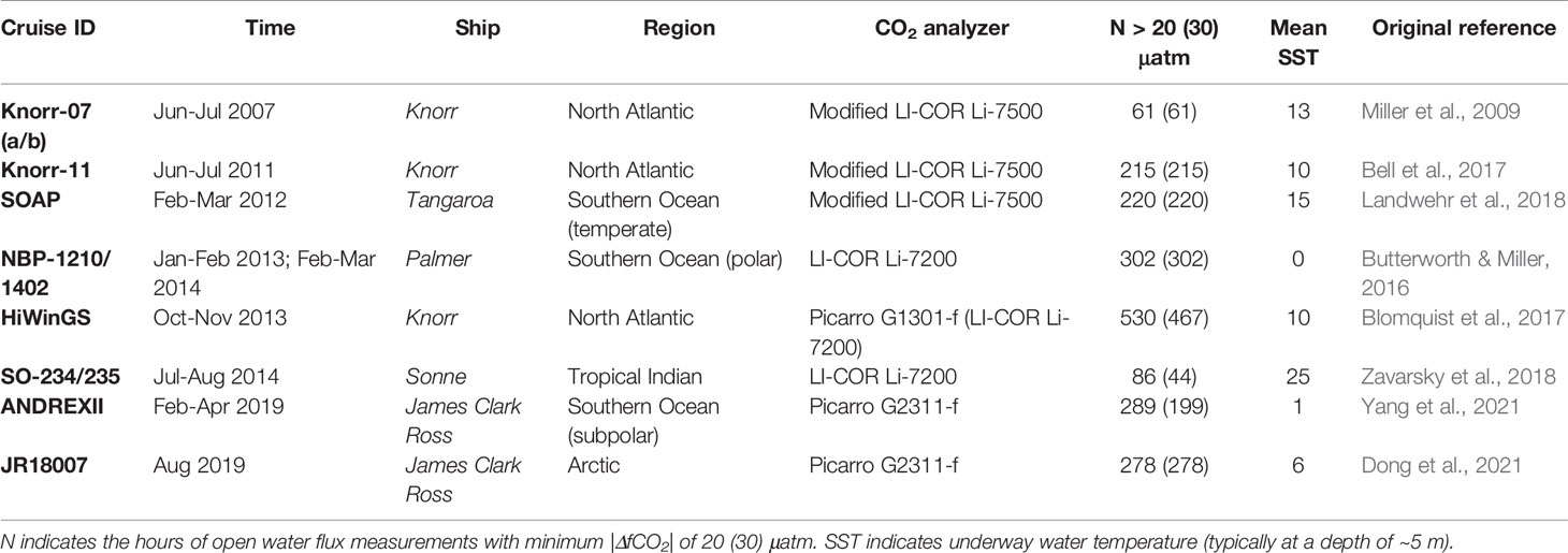
Table 1 Shipboard eddy covariance CO₂ gas transfer measurements using closed-path infrared analyzers (LI-COR Li-7200 or modified LI-COR Li-7500) or cavity ringdown analyzers (Picarro G1301-f, G2311-f) with a physical dryer.

FIGURE 1

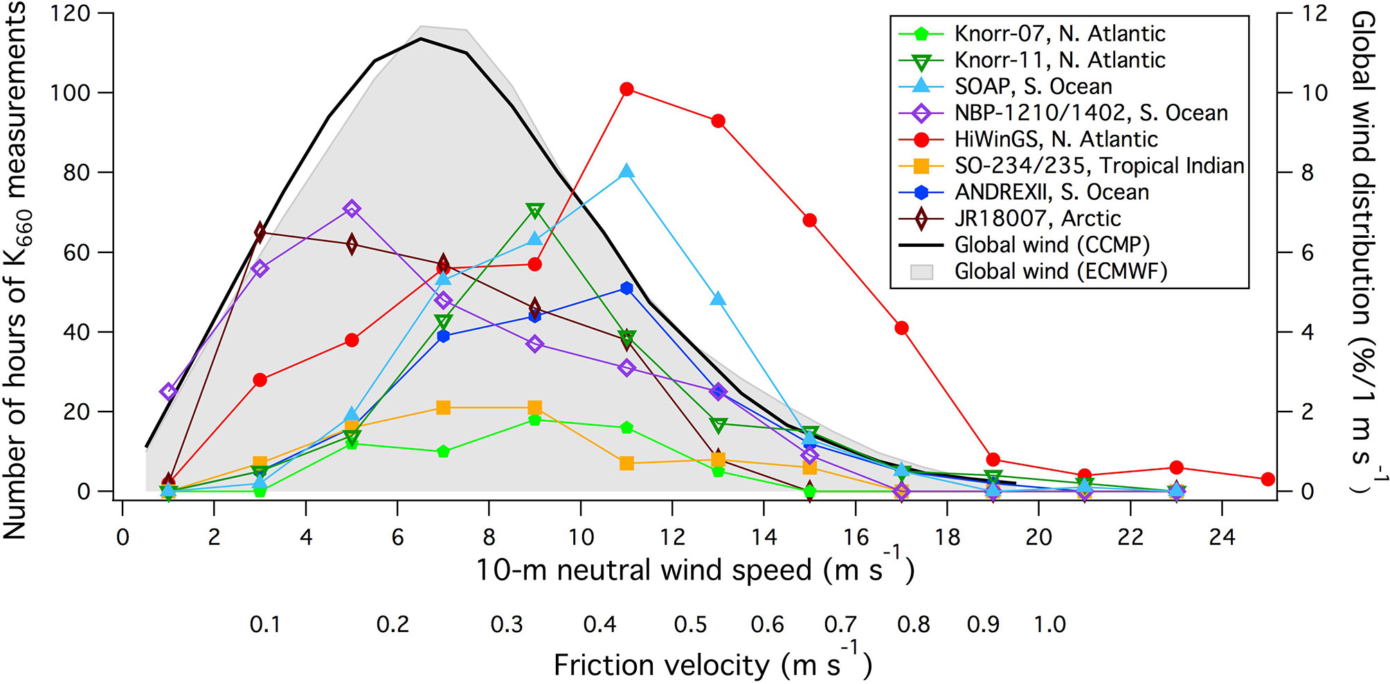
Figure 1 Hours of K₆₆₀ measurements from eight datasets (11 cruises) at different wind speeds and the global wind distributions. The approximate u_* values are shown on the bottom of the plot.

All the cruises above used a closed-path CO₂ analyzer (LI-COR or Picarro cavity ringdown analyzers) with a Nafion dryer, effectively eliminating the issue of water vapor interference in the CO₂ signal and the need for a Webb correction (e.g., Landwehr et al., 2014; Blomquist et al., 2014). We do not consider data from the earlier GasEx studies in this reevaluation. The SO GasEx (Edson et al., 2011) cruise used an open-path LI-COR CO₂ analyzer with known water vapor interference (Landwehr et al., 2014; Blomquist et al., 2014). GasEx98 (Wanninkhof and McGillis, 1999; McGillis et al., 2001) and GasEx01 (McGillis et al., 2004) used a closed-path LI-COR CO₂ analyzer but without a dryer. Observations by Prytherch et al. (2017) near sea ice used a Fast Greenhouse Gas Analyzer (Los Gatos Research), which is substantially noisier than the closed-path LI-COR and Picarro cavity ringdown analyzers and thus resulted in a much greater flux uncertainty (Yang et al., 2016); those observations are also not considered in this analysis.

Cruise data were supplemented with model U_10n data provided by the ECMWF global reanalysis (ERA-5) and ocean wave data from a hindcast based on ERA-5 forcing (ERA-5H). The ERA-5 reanalysis provides a comprehensive record of the global atmosphere, land surface, and ocean waves from 1950 onwards. Compared with the previous reanalysis (ERA-Interim), ERA-5 benefits from over a decade of research and development in model physics, core dynamics, and data assimilation. The reanalysis also offers an increase in horizontal resolution (31 km) and time resolution (1 hour), as well as an increase in the vertical atmospheric model levels. The ERA-5 output was produced with ECMWF IFS Cy41r2, used for the operational forecast from March 8 to November 2016. For more details, please refer to Hersbach et al. (2020).

Even though ERA-5 has an ocean wave component, in this study we use wave data from an hindcast (ERA-5H). This hindcast is based on a more advanced version of ECMWF wave prediction system ecWAM (Cy47r1; ECMWF, 2020). The ERA-5H is a long global wave model simulation (1979-2020), forced by ERA-5 hourly 10-m neutral winds, surface air density, gustiness, and sea ice cover. The latter is used to prevent wave generation and propagation in all areas with the sea ice cover >30%. Like ERA-5, the output of ERA-5H is hourly, but it has finer spatial (~20 km) and spectral resolutions (ERA-5: 24 directions, 30 logarithmically spaced frequencies, last frequency ~0.56 Hz; ERA-5H: 14 km, 36 directions and 36 frequencies, last frequency ~1 Hz). The ERA-5H benefits from an updated wave physics for wind input and swell dissipation (based on the work of Ardhuin et al., 2010) and has been successfully incorporated into the operational ecWAM wave model component of IFS (Bidlot, 2019).

Model data are collocated with the cruise data using a bi-linear interpolation in space and a linear interpolation in time. For the purpose of this study, the total significant wave height (H_s) and the mean squared slope (MSS) of the waves from the model are used (see ECMWF, 2020 for further details). It is important to note that the MSS here is determined with the high frequency cut-off given by the model discretization (~1 Hz).

2.2 Reevaluation Methods

EC CO₂ flux data are reevaluated to ensure comparability. Significant changes to some of the original data include:

- CO₂ flux data averaged to hourly interval (minimum of 40 minutes required per hour) following recommendation by Dong et al. (2021)

- Solubility and Schmidt number computed following the equations given by Wanninkhof (2014)

- Air-sea CO₂ concentration difference computed with consideration of the skin temperature effect (see Eq. 4 below)

The cool skin effect is accounted for when computing the gas transfer velocity:

$\begin{array}{ll}{K}_{660}={\rho }_{dry} \overline{w^{\prime }{X}_{C{O}_2}^{\text{'}}}{\left({\text{fCO}}_{2\text{w}}So{l}_{bulk}–{\text{ fCO}}_{2\text{a}}So{l}_{skin}\right)}^{-1}{\left(660/Sc\right)}^{-0.5}& (4)\end{array}$

The CO₂ solubility at the skin temperature (Sol_skin) is used to calculate the equilibrium atmospheric concentration. The skin temperature is estimated from the COARE3.5 model using underway water measurements and meteorological observations as inputs (see e.g., Fairall et al., 1996 and Zhang et al., 2020 for validation of the modeled cool skin temperature effect). Because Sol_skin is almost always greater than Sol_bulk, relative to the original analyses (Eq. 2) the inclusion of the cool skin effect reduces K₆₆₀ slightly during CO₂ invasion, and increases K₆₆₀ slightly during CO₂ evasion. For example, at a fCO_2a value of 400 μatm and a cool skin effect of 0.17°C, the difference between ΔC with consideration of cool skin (fCO_2w Sol_bulk – fCO_2a Sol_skin) and the ‘traditional’ ΔC (Sol_bulk (fCO_2w – fCO_2a)) equates to about 2 μatm. If Sol_bulk (fCO_2w – fCO_2a) is –30 μatm, consideration of the cool skin reduces K₆₆₀ by ~7%. Note that to ensure comparability with previous publications, Sc here is computed using the bulk, rather than skin, temperature. Using the skin temperature to compute the Schmidt number would generally increase K₆₆₀ by ~0.5% (see Woolf et al., 2016 for further discussion on this detail).

Woolf et al. (2016) suggested that in the presence of a diurnal warm layer, the bulk underway temperature will be different from the temperature at the base of the thermal diffusive layer (i.e., subskin temperature at ca. 1 mm depth). We have assumed a negligible diurnal warm layer effect and assume that underway water temperature is equal to the subskin temperature for two reasons. First, in-situ skin (or subskin) temperature was rarely measured on these cruises, while match ups with satellite skin (or subskin) temperatures are very rare. Two, measurements of subskin temperature using a floating thermistor (aka the NOAA “sea snake”) during HiWinGS and SO GasEx suggest that for open ocean at mid/high latitudes, the diurnal warm layer effect is small (see Supplementary Figures 2, 3). Note that near surface temperature gradients might have been more important for the tropical cruises SO-234/235.

Original references for HiWinGS and for SO-234/235 included data where |ΔfCO₂| was as low as ~20 μatm. Selecting an appropriate |ΔfCO₂| threshold is important for minimizing random uncertainty as well as bias in K₆₆₀. As shown by Dong et al. (2021), the bottom-up uncertainty in K₆₆₀ (derived from uncertainty in EC flux and dominated by random uncertainty) increases significantly when |ΔfCO₂|< 20 μatm. At wind speeds < ~6 m s^-1, a more stringent threshold of 30 μatm is needed to maintain a reasonable signal:noise ratio. In addition, any bias in the air-sea CO₂ concentration difference (e.g., due to measurement uncertainty or unaccounted for near surface temperature gradients) would have a proportionally greater impact on K₆₆₀ at low |ΔfCO₂| values. For example, uncertainty in fCO_2w from the Surface Ocean CO₂ Atlas (Bakker et al., 2016) is often taken to be ~2 μatm. A total uncertainty in air-sea CO₂ gradient of 3 μatm (considering similar contribution from errors due to fCO₂a and temperature) would contribute to a relative uncertainty in K₆₆₀ of ~15% at |ΔfCO₂| = 20 μatm. A more stringent |ΔfCO₂| threshold reduces the amount of data available, and so the reanalyzed HiWinGS and SO-234/235 data are presented with minimum |ΔfCO₂| of both 20 and 30 μatm.

For most cruises, we use the bulk u_* computed with the COARE3.5 model from the least distorted shipboard wind speed measurement. Note that this bulk u_* is largely a function of wind speed and atmospheric stability, and does not explicitly consider the impact of waves. For SOAP, the EC system was positioned lower and closer to ship’s bow, which caused significant flow distortion (Landwehr et al., 2018). The authors estimated U_10n from the EC u_* using the COARE3.5 u_* vs. U_10n relationship, but the corrected U_10n still tends to be higher than the ECMWF data except at the highest wind speeds (see Table 2). For the SO-234/235 cruises, where the EC system was also positioned lower, the in-situ U_10n tends to be higher than the ECMWF data except at the lowest wind speeds. While the ECMWF U_10n estimates are not exempt from bias, this comparison implies that the K₆₆₀ vs. u_* relationships for SOAP and SO-234/235 could be subject to an additional U_10n-driven uncertainty of ~10%.

TABLE 2

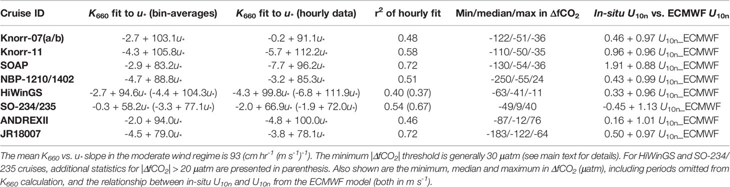
Table 2 Regression analyses between CO₂ K₆₆₀ (in cm hr^-1) and friction velocity (in m s^-1) between u_* values of 0.1 and 0.5 m s^-1.

3 Results

To facilitate the interpretation of the large number of data points from all cruises (~2000 hours of K₆₆₀ observations), this work focuses on the statistics (e.g., mean, standard deviation, standard error) of binned hourly K₆₆₀ values. The standard deviation is used to illustrate variability, while the standard error reflects the accuracy in the measurement. The hourly data from each cruise are included in the supplement for interested readers.

3.1 Moderate Winds

We first look at K₆₆₀ data at moderate wind speeds (u_* 0.1-0.5 m s^-1, or U_10n of approximately 3-13 m s^-1), which encompasses the majority of the measurements (Figure 1). We choose u_* as the default independent parameter for assessing the variability in K₆₆₀, in accordance with the custom of similarity theory. K₆₆₀ scales approximately linearly with u_* within this range (Figure 2). We note that much of the HiWinGS data at intermediate wind speeds were collected during the decline of intense storms, when the waves were much larger than typically observed at those windspeeds. This probably led to enhanced transfer. See Section 3.3 for further discussion about waves.

FIGURE 2

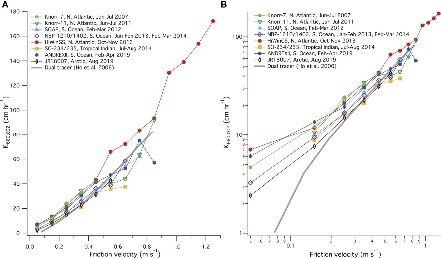
Figure 2 (A) K₆₆₀ averaged to friction velocity (u_*) bins in linear scale; (B) the same but in log-log scale. Also shown is the dual tracer relationship from Ho et al., 2006.

The regression statistics, computed both from the bin-averaged K₆₆₀ as well as from hourly K₆₆₀ data, are shown in Table 2. The r² value in the hourly K₆₆₀ fit to u_* tends to be higher for more localized cruises (e.g., SOAP and JR18007) and lower for cruises spanning a large spatial (e.g., NBP-1210/1402, ANDREXII) or temporal (e.g., HiWinGS) range. The mean in the K₆₆₀ vs. u_* slopes in the moderate wind regime is about 93 (cm hr^-1 (m s^-1)^-1), with a relative standard deviation of ~15% and a range of ~40%. The steepness in the K₆₆₀ vs. u_* slopes appears to follow a general trend of North Atlantic ≥ Southern Ocean > Arctic and tropical Indian. The K₆₆₀-U_10n relationships are similar to the K₆₆₀-u_* relationships in spatial distribution but are less linear (Supplementary Figure 4).

Any bias in the K₆₆₀ vs. u_* (or U_10n) relationships could be due to biases in u_* (or U_10n), in the EC flux, or in the air-sea concentration difference. The slope between in-situ derived U_10n and U_10n from the ECMWF model is within 4% from unity (relative standard deviation of 2.5%), with the exception of SOAP and SO-234/235 (see Reevaluation Methods). The good agreement implies that any bias in the in-situ u_* (or U_10n) data (e.g., due to flow distortion) is generally small. Plotting K₆₆₀ against U_10n from ECMWF does not substantially change the mean K₆₆₀ vs. U_10n relationships (Supplementary Figure 4).

The quasi-linearity between K₆₆₀ and u_* at moderate wind speeds allows us to assess possible biases in flux and in the air-sea concentration difference. Data at low |ΔfCO₂|, typically discarded in the calculation of K₆₆₀, are particularly useful for evaluating such biases. Normalizing the measured EC flux for the kinetic forcing, here we define a new term:

$\begin{array}{ll}\text{Akinetic flux}=Flu{x}_{CO2}\hspace{0.17em}{u}_{*}^{-1}{\left(660/Sc\right)}^{-0.5}=\Delta C\hspace{0.17em}{K}_{660}\hspace{0.17em}{u}_{*}^{-1}& (5)\end{array}$

The akinetic flux is plotted against ΔC (Figure 3), including the low |ΔfCO₂| data that are often-discarded. It is apparent that the akinetic flux from all cruises follow a broadly similar trend ($\text{slope}=K_{660}\hspace{0.17em}{u}_{*}^{-1}$, the dimensionless transfer coefficient; Jähne et al., 1987). For cruises with both positive and negative concentration differences (NBP1210/1402, ANDREXII, and SO-234/235), the akinetic flux approximately goes through the origin. The fact that the EC flux is roughly zero when the concentration difference is zero suggests that both the flux and concentration measurements do not suffer from large bias. From this, we conclude that the variability in the mean K₆₆₀ vs. u_* relationships among different cruises is not primarily due to measurement uncertainties.

FIGURE 3

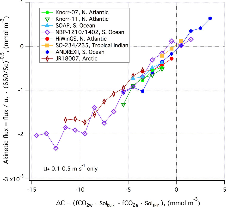
Figure 3 Akinetic flux vs. the air-sea concentration difference in moderate winds.

Figure 4 shows the variability and uncertainty in K₆₆₀ within this dataset. For individual cruises, standard deviation (standard error) is computed from hourly K₆₆₀ data within u_* bins. Relative standard deviation (relative standard error) is the standard deviation (standard error) above divided by the bin-averaged K₆₆₀. Similar statistics are also computed from the bin-averaged K₆₆₀ (black lines). While standard error in K₆₆₀ tends to increase with u_* (as expected), the relative standard error is at its minimum in moderate winds (generally within 10%). The lowest and highest wind speed bins for each cruise have the smallest sample sizes, which contribute to larger relative standard error. The next sections will focus on K₆₆₀ in the low and high wind speed regimes.

FIGURE 4

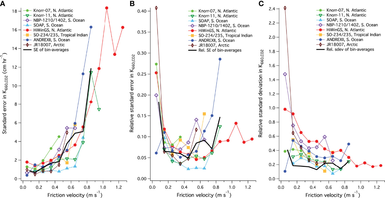
Figure 4 (A) standard error in hourly K₆₆₀ for each cruise (colored markers) and the standard error of the bin-averages for all the cruises (black line); (B) the same but showing the relative standard error in hourly K₆₆₀; (C) the same but showing the relative standard deviation in hourly K₆₆₀. Standard deviation here is approximately the root mean squared error, not mean absolute error.

3.2 Low Wind Regime

Gas exchange at low wind speeds (u_* <0.25 m s^-1, or U_10n < 7 m s^-1) has received relatively little attention over the last decade. Figure 4 shows that the relative uncertainty (both relative standard error and relative standard deviation) in K₆₆₀ of CO₂ is the largest at low winds. This is partly caused by the increase in the turbulent integral time scale at low wind speed, which increases the EC sampling error. Large relative uncertainty at low wind speeds is observed in fluxes of CO₂ (Dong et al., 2021) as well as in momentum and heat (Blomquist et al., 2014). In addition, processes other than wind that affect gas exchange (e.g., chemical enhancement, surfactants, convection) probably contribute more significantly towards the variability in K₆₆₀ at low winds.

The absolute uncertainty in K₆₆₀ at low winds is small, and the bin-averaged K₆₆₀ from all of the cruises significantly exceeds the dual tracer parametrization (Ho et al., 2006) by a few cm hr^-1 at u_* below 0.25 m s^-1 (Figure 2). This amounts to a mean difference of ~75% at u_* of 0.15 m s^-1. There are several possible reasons for this discrepancy between dual tracer and EC-derived K₆₆₀: a) very few dual tracer measurements of K₆₆₀ over the ocean were made at low wind speeds, with only two points below a wind speed of 5 m s^-1 in Ho et al., 2006; b) the quadratic fit of dual tracer K₆₆₀ was forced through the origin; c) chemical enhancement, we discuss below. Physical considerations lead us to expect some gas transfer even at very low wind speeds. For example, Mackay and Yeun (1983) estimate the ‘still air’ K₆₆₀ to be ~0.4 cm hr^-1. Convective turbulence related to heat fluxes may further enhance K₆₆₀ under calm conditions, and the COARE3.0 model estimates this to contribute ~2 cm hr^-1 at typical (slightly unstable) oceanic conditions (see e.g., Yang et al., 2011).

Furthermore, unlike the dual tracers ³He and SF₆, the air-sea exchange of CO₂ is subject to chemical enhancement due to carbonate equilibrium kinetics (faster in warmer waters, e.g., Soli and Byrne, 2002). Based on the film model of Hoover and Berkshire (1969) and carbonate kinetics, Wanninkhof (1992) estimated the chemical enhancement of CO₂ to be on the order of 2 cm hr^-1. Jähne et al. (2010) derived a similar value for chemical enhancement by concurrently measuring the exchange of N₂O (no chemical enhancement) and CO₂ in a wind-wave tank. The enhancement was found to be well described by a surface renewal model that incorporates carbonate kinetics. Considering together the field and laboratory evidence as well as theoretical understanding, it is highly likely that using the dual tracer parametrization of K₆₆₀ (e.g., Ho et al., 2006) will result in an underestimation of air-sea CO₂ exchange at low wind speeds.

The computed K₆₆₀ from EC CO₂ fluxes could be even greater at low wind speeds if we assume a different Schmidt number scaling. Liss and Merlivat (1986) found that the wind speed dependence in K₆₆₀ is weaker within the smooth surface regime (below U_10n of 3.6 m s^-1 per their definition), where gas exchange is dominated by waterside diffusive processes. They suggested that K₆₆₀ should be scaled with Sc^-2/3 within this smooth regime; then once waves appear the Schmidt number exponent transitions to -1/2. Recent laboratory (Nagel et al., 2019) and field (Esters et al., 2017) observations imply that there is a smooth transition in n between -2/3 and -1/2. The intercepts of the K₆₆₀-u_* fits (over u_* range of 0.1-0.5 m s^-1) are negative for all cruises (Table 2), which implies different physical processes occurring at low wind speeds. All cruises (except for SO-234/235) took place in waters less than 20 °C (the temperature where Sc of CO₂ = 660). Scaling to K₆₆₀ from K with Sc^-2/3 instead of Sc^-1/2 would lead to an increase in K₆₆₀ by ~10% (from SST = 10 °C) to ~20% (from SST = 0 °C), and bring the intercept in the K₆₆₀-u_* relationship closer to zero. In Supplementary Figure 5, K₆₆₀ normalized using a variable Schmidt number exponent (Esters et al., 2017) is shown, which can be compared against Figure 2. We retain the Sc^-1/2 scaling for the rest of this work to ensure comparability with previous dual tracer and ¹⁴C analyses and provide the K data at ambient SST in the supplement.

It is worth repeating that accounting for the cool skin effect (i.e., use of Eq. 4 instead of Eq. 2 and 3) increases the magnitude of ΔC and thus reduces the derived K₆₆₀ of CO₂ in regions of CO₂ invasion. Vertical gradients in fCO_2w between the depth of water sampling (typically ~5 m) and the subskin due to diurnal warm layer formation may occur under calm conditions and strong solar irradiance. We have not explicitly considered warm layer in this analysis due to a paucity of near surface temperature observations, incomplete input variables needed for modeling the warm layer (e.g., solar flux missing for several cruises), and uncertainty in the model (Fairall et al., 1996). To illustrate an order of magnitude effect, the global mean daytime difference between the subskin and ~5 m depth is about 0.08°C at U_10n = 5 m s^-1 based on NOAA’s long-term shipboard measurements between 70°N and 60°S. This corresponds to an isochemical change (i.e., constant alkalinity and total dissolved inorganic carbon; Woolf et al., 2016) in fCO_2w of about 1.4 μatm. The effect of warm layer on ΔC is thus similar in magnitude to the cool skin effect at this wind speed, but in the opposite direction. Inclusion of any warm layer effect in regions of CO₂ invasion would thus increase the derived K₆₆₀ of CO₂ by ~5% at |ΔfCO₂| = 30 μatm. Large swaths of the global oceans experience low wind speeds. Given the uncertainty surrounding the various concurrent physical processes, gas exchange under these conditions requires further investigation (e.g., a dedicated research campaign in calm conditions, similar to GasEx01 but with improved flux methodology and a thorough examination of the surface temperature profile).

3.3 High Wind Regime and Waves

A number of studies over the last decade have focused on gas exchange at high wind speeds (especially HiWinGS), where K₆₆₀ is considered to be the most uncertain. As shown in Figure 4, at u_* above 0.5 m s^-1 the standard errors in K₆₆₀ (absolute and relative) for individual cruises as well as for bin-averages of all cruises do increase in high winds. In contrast, the relative standard deviation does not increase with wind speed. This is likely in part because the relative uncertainty in EC CO₂ flux tends to decrease with increasing wind speed, presumably due to better sampling statistics (i.e., more turbulent eddies blowing past the sensor within a given averaging time; see Dong et al., 2021). Thus, the perceived large uncertainty in K₆₆₀ in high winds can at least be partly attributed to the paucity of observations. More measurements under those extreme conditions will improve the accuracy in K₆₆₀.

What does this large dataset tell us about the effect of wave breaking and bubble-mediated gas exchange on K₆₆₀? Following Woolf (1997) and the COARE model (Fairall et al., 2011), CO₂ gas transfer velocity is often thought to be the sum of diffusive (i.e., interfacial) gas exchange (scaled with u_*) and bubble-mediated gas exchange. Bubble-mediated exchange, scaled with the whitecap fraction, is judged to be the reason why CO₂ transfer is much faster than DMS transfer at high wind speeds (e.g., Bell et al., 2017) and has been estimated to be dominant exchange pathway for CO₂ in rough seas (e.g., Blomquist et al., 2017). The whitecap fraction is long thought to have a cubic wind speed dependence, but observations during HiWinGS at wind speeds up to ~ 24 m s^-1 show an overall windspeed dependence in whitecap fraction that is much weaker than cubic (Brumer et al., 2017a). This might be one reason why the u_* (and U_10n) dependence in K₆₆₀ of CO₂ is closer to linear than to cubic (Figure 2 and Supplementary Figure 4).

Another possibility for the near linear dependence in K₆₆₀ of CO₂ on u_* could be saturation in diffusive gas exchange at very high wind speeds. This phenomenon has sometimes been observed in the more soluble gas dimethyl sulfide (DMS), e.g., during SO GasEx as described by Blomquist et al. (2017) and during Knorr-11 as described by Bell et al. (2013), and it could partly compensate for the rapid increase in bubble-mediated gas exchange with wind. In the following, we explore the use of wave parameters, rather than whitecap fraction, to represent the effects of wave breaking and bubbles on K₆₆₀.

Figure 5 shows the distribution of significant wave height (H_s) for all the cruises. HiWinGS in the North Atlantic and ANDREXII in the sub-polar Southern Ocean (two cruises with high K₆₆₀:u_*; see Table 2) experienced some of the largest waves at moderate to high wind speeds (also see Supplementary Figure 6). In contrast, NBP-1210/1402 in the polar Southern Ocean and JR18007 in the Arctic (two cruises with low K₆₆₀:u_*; see Table 2) often encountered small waves, possibly due to the close proximity of sea ice and thus shorter fetch. For context, Figure 5 also shows the global distribution in H_s from ECMWF ERA5 (0.5° hourly resolution data; Hersbach et al., 2018), here approximated from 12 evenly spaced days in year 2020 (e.g., 1^st January, 1^st February, 1^st March…). H_s data from the individual cruises span from below to above the global distribution.

FIGURE 5

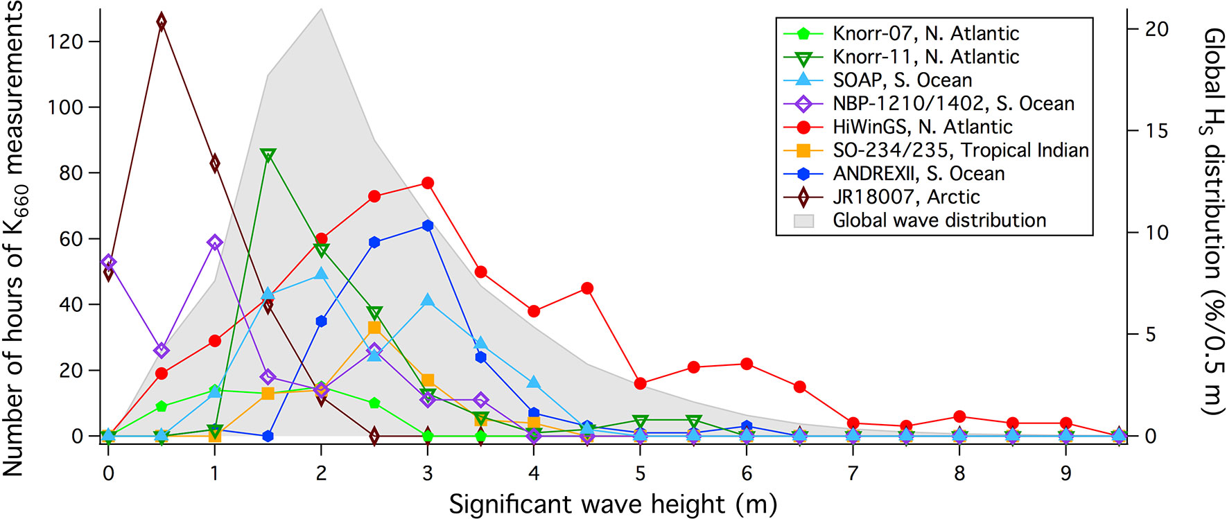
Figure 5 Hours of K₆₆₀ measurements at different significant wave heights and the global distribution of significant wave height from ECMWF.

FIGURE 6

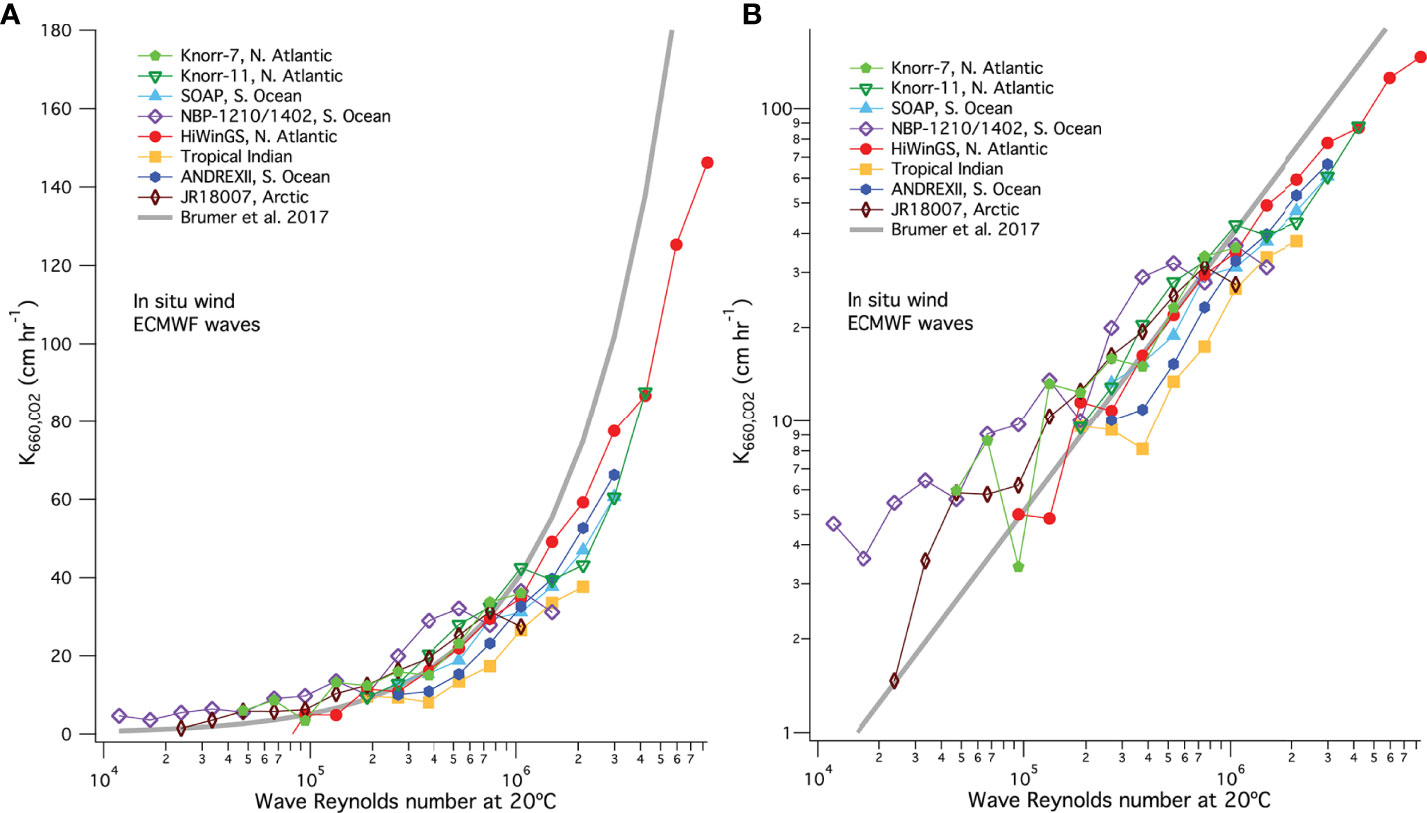
Figure 6 K₆₆₀ averaged into bins of R_Hw (20 °C) in semi-log scale (A) and log-log scale (B).

Brumer et al. (2017b) suggested the K₆₆₀ is better parameterized as a function of the wave Reynolds number (R_Hw = H_s u_*v^-1) than as a function of wind speed, where v is the viscosity of seawater. K₆₆₀ is plotted against the wave Reynolds number (R_Hw) in Figure 6. Here H_s from the ECMWF model and seawater viscosity at 20°C (rather than ambient temperature) are used to compute R_Hw for all cruises. Using ambient water viscosity substantially increases the discrepancy in the K₆₆₀-R_Hw relationships between polar and temperate cruises.

It appears that R_Hw does help to collapse the variability in K₆₆₀ among the different cruises in very heavy seas (i.e., R_Hw > 10⁶). For example, the relative standard deviation in K₆₆₀ among HiWinGS, SOAP, ANDREXII, and Knorr-11 at R_Hw between 2 • 10⁶ and 3 • 10⁶ is 12-14%. In comparison, the relative standard deviation at u_* above 0.5 m s^-1 is about 20% for these cruises (Figure 4). Note that the K₆₆₀ data from all cruises fall below the Brumer et al. (2017b) parametrization $\left(K_{660}=2.04·{10}^{-4}{R}_{Hw}^{0.88}\right)$ in heavy seas because that parametrization was largely developed from the original HiWinGS K₆₆₀ data. Those data were overestimates due to an incorrect treatment of CO₂ solubility.

In less extreme seas (i.e., R_Hw < 10⁶), R_Hw explains less of the variability in K₆₆₀ than u_*. For example, the relative standard deviation in bin-averaged K₆₆₀ among all cruises at R_Hw of 3.8 • 10⁵ is 38%. Possible explanations for this include a) R_Hw is an imperfect descriptor of wave breaking, especially for small scale waves, and b) breaking of large-scale waves and bubble-mediated processes become dominant for CO₂ gas exchange only in very heavy seas, whereas gas exchange at lower wind speeds is dominated by diffusive transfer.

The mean squared slope (MSS) of the waves incorporates to an extent the combined effect of wind and smaller-scale waves. Frew et al. (2004) observed that K₆₆₀ consistently correlates better with MSS than with wind speed at a coastal location at fairly low wind speeds. Figure 7 shows the CO₂ K₆₆₀ vs. MSS from the ECMWF model (integrated up to 1 Hz) as well as vs. the ECMWF U_10n. In small to moderate seas, MSS explains slightly more variance in K₆₆₀ than U_10n. For example, between MSS of 0.025 to 0.04, the relative standard deviation in K₆₆₀ averaged in MSS bins among all cruises is ~15%. In comparison, the relative standard deviation as a function of ECMWF U_10n is close to 20% at moderate wind speeds of ~10 m s^-1. In rougher seas, the advantage of using MSS over U_10n, u_*, or R_Hw to parametrize is K₆₆₀ less obvious.

FIGURE 7

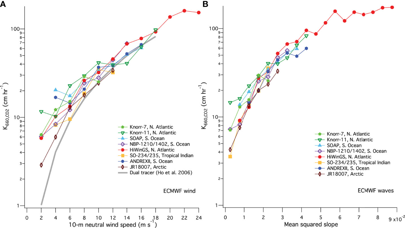
Figure 7 (A) K₆₆₀ averaged into bins of ECMWF U_10n; (B) K₆₆₀ averaged into bins of ECMWF mean squared slope (MSS).

The regional variability in the K₆₆₀-u_* relationships is less apparent in the K₆₆₀-R_Hw and K₆₆₀-MSS relationships, which implies that variations in waves in different ocean basins contribute towards the regional variability in K₆₆₀. A logical future step for extrapolating the K₆₆₀ data to the global oceans may be to develop a wind/wave-dependent parametrization of K₆₆₀ (e.g., as a function of R_Hw and MSS). However, in the next section we take the simpler approach of computing the grand average K₆₆₀-u_* relationship and combining it with the global wind speed distribution. The resultant global average K₆₆₀ implied from EC CO₂ flux measurements is then compared against tracer-based estimates.

4 Comparison to Tracer-Based Estimates and Implications on the Global CO₂ Flux

A fairly robust constraint for global average air-sea CO₂ exchange is the ¹⁴C disequilibrium. Wanninkhof (1992) combined an estimate of this value with the global mean wind speed and assumed a quadratic wind speed dependence (with no gas exchange at U_10n = 0) to develop a widely used K₆₆₀ parametrization. The ¹⁴C-based global average K₆₆₀ value has since been reassessed by Naegler et al. (2006); Krakauer et al. (2006); Sweeney et al. (2007), and Müller et al. (2008). Accordingly, the ¹⁴C tracer based K₆₆₀ parametrization has been updated by Wanninkhof (2014). Naegler (2009) further corrected the global average K₆₆₀ estimates upwards by accounting for the changing oceanic radiocarbon inventory due to CO₂ uptake and using realistic reconstructions of sea surface ¹⁴C disequilibrium.

Our study incorporates over 2000 hours of EC K₆₆₀ data from 11 cruises around different parts of the global oceans. Is the overall mean of these observations representative of the global average and how does that compare to the tracer data? The grand average of EC K₆₆₀ data (average of the bin averages) from all cruises is shown in Figure 8. The polynomial fits of this data to u_* and to U_10n, weighted by the standard error in each bin, are $K_{660}=-1.47+76.67u_{*}+20.48u_{*}^2\text{\hspace{0.17em}and\hspace{0.17em}}{K}_{660}=0.36+1.203U_{10n}+0.167U_{10n}^2$, respectively (K₆₆₀ in cm hr^-1; u_* and U_10n in m s^-1). A power fit of the grand average as a function of wind speed yields an exponent that is less than two: $K_{660}=1.92+0.57U_{10\text{n}}^{1.68}$. The relative standard error is ~7% and the relative standard deviation of our grand average is ~19% at moderate wind speeds. We note that for users who wish to apply the above equations to estimate CO₂ fluxes, the cool skin effect should be taken into account in the calculation of ΔC and the Schmidt number should be computed at the subskin, rather than skin, temperature.

FIGURE 8

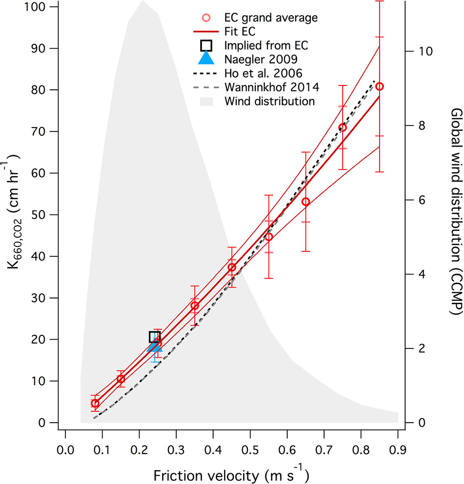
Figure 8 Grand average of EC K₆₆₀ from all cruises vs. friction velocity, with the smaller (larger) error bars indicating standard error (standard deviation). The thick red line indicates the weighted polynomial fit to this data $\left(K_{660}=-1.47+76.67u_{*}+20.48u_{*}^2\right)$, while the thin red lines are the 95% confidence bands for the fit. Combining the grand average of EC K₆₆₀ with the CCMP wind distribution yields a global average K₆₆₀, which is shown along with the Naegler (2009) estimate. Also shown are previous K₆₆₀ relationships from Wanninkhof (2014) based on ¹⁴C disequilibrium and from Ho et al. (2006) based on the dual tracer (³He/SF₆) method.

To compute a global average K₆₆₀ from EC observations, we primarily utilize the global Cross-Calibrated Multi-Platform (CCMP) wind speed distribution (0.25°, 6-h resolution; Atlas et al., 2011), which was used by Wanninkhof (2014) to develop the ¹⁴C-based K₆₆₀ parametrization. Combining the grand average of EC K₆₆₀ as a function of u_* with the CCMP wind speed distribution (transformed to u_* according to the COARE 3.5 stress relationship), we get a global average K₆₆₀ implied from EC observations of 20.6 cm hr^-1, with a standard error (standard deviation) of 1.5 (3.9) cm hr^-1. This global average is well within the range and uncertainties of the corrected global average values (18.2 ± 3.6 cm hr^-1) reported by Naegler (2009) based on ¹⁴C disequilibrium (Figure 9). Using the ECMWF ERA5 global wind speed distribution (0.25°, 1-h resolution; Hersbach et al., 2020) instead, we get a slightly lower global average, EC-implied K₆₆₀ of 19.7 cm hr^-1. This was estimated by applying the coefficients provided in by Fay et al. (2021, Table A2) to the CCMP-based K₆₆₀.

FIGURE 9

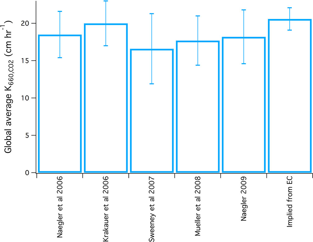
Figure 9 Global average K₆₆₀ estimates from ¹⁴C (see Naegler, 2009) and implied from EC measurements, the latter based on CCMP wind distribution. The error bar on the EC estimate represents standard error.

Some regions of the global oceans are missing (e.g., most of the Pacific Ocean) from or underrepresented (e.g., tropics) in this analysis. We have chosen to omit coastal measurements from stationary sites, which may be more affected by spatial heterogeneity in the flux footprint (e.g., Yang et al., 2019), fetch (e.g., Prytherch and Yelland, 2021), and different wave breaking characteristics compared to the open ocean. Furthermore, there are some differences between the grand average H_s from all the cruises and the global average H_s in high winds (see Supplementary Figure 6). Nevertheless, Figures 8, 9 suggest that the grand average of EC K₆₆₀ from the 11 cruises is a reasonable representation of the global average air-sea CO₂ exchange.

The tracer-based K₆₆₀ parametrizations (Wanninkhof, 2014 and Ho et al., 2006) are noticeably lower (i.e., below the 95% confidence bands) than the grand average of EC K₆₆₀ data at low wind speeds (Figure 8). As discussed in Section 3.2, this discrepancy likely relates to the early assumption of no gas exchange at U_10n = 0. In moderate to high winds, the tracer-based estimates are within the confidence bands of the EC K₆₆₀ grand average.

Based on the CCMP global wind distribution, the implied global average K₆₆₀ from EC CO₂ measurements is about 20% higher than the dual tracer estimate from Ho et al. (2006). Adjusting K₆₆₀ upwards at low wind speeds but not at high wind speeds will affect the spatial and temporal variability in estimated CO₂ fluxes. The lower latitude oceans are typically regions of net CO₂ emission and tend to have fairly low wind speeds. Meanwhile, in temperate/high latitudes, the spring phytoplankton bloom usually coincides with shoaling of the ocean mixed layer that is in part aided by a seasonal reduction in wind speed. Our results suggest that previous estimates of CO₂ emission and uptake in such instances could be underestimated.

5 Looking Forward

Overall, the relative uncertainty in K₆₆₀ is largest at very low wind speeds (Section 3.2), while the absolute uncertainty is largest at very high wind speeds (High Wind Regime and Waves). Despite combining 11 cruises, data during these extreme conditions remain scarce (Figure 1) and should be the foci of future field projects. Future measurements in the tropics and in the Pacific Ocean should further improve the representativeness of the grand average EC K₆₆₀ and aid the development of a wind/wave-dependent parametrization of K₆₆₀.

One of the key advantages of the EC technique is the ability to capture variability in K₆₆₀ on much shorter timescales (one to a few hours; see Dong et al., 2021) than tracer-based approaches (days to years). EC is thus well suited for studying the more ephemeral processes that affect air-sea exchange. The analysis presented here has taken the approach of bin-averaging K₆₆₀ data in various parameter spaces (e.g., u_*, U_10n, R_Hw, and MSS). This approach is useful for reducing measurement noise but could have the undesirable effect of averaging out the processes of interest. Hourly data from all the cruises are included in the supplement. Future analysis of this dataset (plus any additional datasets) on shorter timescales (e.g., without bin-averaging) may illuminate further process-level insights.

Consideration of waves helps to explain some of the variability that is not accounted for by U_10n (or by a U_10n dependent formulation of u_*). Future EC K₆₆₀ measurements should clearly be accompanied by high resolution wave measurements (such as during Knorr-11 and HiWinGS). At low to moderate wind speeds, given the fact that K₆₆₀ is more scattered vs. ECMWF U_10n (Figure 7) than vs. in-situ U_10n (Supplementary Figure 4), it is plausible that an in-situ observation of surface roughness or MSS would be superior to the current model MSS for parametrizing K₆₆₀. Such a measurement possibly also helps to account for the dampening of smaller-scale waves by surfactants (Frew et al., 2004). Further model development (e.g., Janssen and Bidlot, 2021) extending the MSS estimate to higher frequencies (i.e., including micro-breaking) may also be fruitful. At high wind speeds, the current use of R_Hw ignores any directional difference between wind and wave, which has been proposed to have some influence on gas exchange (Zavarsky and Marandino, 2019). Following Blomquist et al. (2017) and Brumer et al. (2017b), this work only considers H_s of the total waves in the calculation of R_Hw. The supplement of this paper includes hindcast wave data for both wind-sea and swell, permitting a more thorough investigation into the effects of wind-wave directional offset as well as the different influences from wind-sea and swell on gas exchange.

Partitioning the total gas transfer velocity into diffusive and wave-dependent bubble components (following the approaches of e.g., Blomquist et al., 2017; Deike and Melville, 2018), constrained by multiple gases of different solubility, is necessary to further improve process-level understanding in gas exchange. In addition to CO₂ and DMS, concurrent K measurement of another gas (preferably with solubility less than or similar to CO₂) would be particularly useful. Such an approach applied in two different wind-wave facilities at high wind speeds with many tracers spanning a wide range of solubilities suggests that bubble-mediated gas transfer is not significant for gases with similar solubility to CO₂ (Krall et al., 2019). This discrepancy between field and laboratory data needs further investigations. Active thermography (e.g., Frew et al., 2004) represents an alternative method to investigate K (especially diffusive exchange) on a short temporal scale. Though given the low Schmidt number of heat (~9), derivation of K₆₆₀ using this method is very sensitive to the assumption of the Schmidt number exponent.

Our discussion so far has not explicitly considered the impact of surfactants. Recent observations (Sabbaghzadeh et al., 2017; Mustaffa et al., 2020) show large spatial variability in sea surface surfactant concentrations, which in turn affect the rate of gas transfer (Pereira et al., 2018; Yang et al., 2021). Yang et al. (2021) used a novel measurement of the gas transfer efficiency to show that the effect of surfactants on CO₂ K₆₆₀ could be on the order of 30% at a global mean wind speed of 7 m s^-1, with even greater effects at lower wind speeds. Future cruises with EC CO₂ fluxes would benefit from concurrent observations of such controlling factors.

6 Conclusion

In this work, we reevaluate eddy covariance (EC)-derived CO₂ gas transfer velocity (K₆₆₀) estimates from eight datasets (11 research cruises). The reevaluation process unified flux averaging times, applied consistent and updated calculations of solubility and Schmidt number, and considered the ocean cool skin effect. Measurement biases in wind, flux, and ΔC were found to be minor. K₆₆₀ scales approximately linearly with the friction velocity (u_*) in moderate winds, with a relative standard deviation (relative standard error) of about 20% (7%).

EC-derived K₆₆₀ at low wind speeds is relatively uncertain, but consistently exceeds the dual tracer estimate, perhaps due to chemical enhancement in CO₂ exchange and the assumptions of the tracer model. The relative standard error (but not the relative standard deviation) in K₆₆₀ increases substantially as wind speed becomes higher. This suggests the perceived large uncertainty in K₆₆₀ in high winds is at least in part due to a paucity of observations.

The steepness in the K₆₆₀-u_* slope demonstrates some regional variability (North Atlantic ≥ Southern Ocean > Arctic, Tropics), and this variability was not primarily due to measurement uncertainties. Compared to wind speed or u_*, the modeled wave Reynolds number (R_Hw, a proxy for breaking of largescale waves) helps to collapse some of the variability in K₆₆₀ in very heavy seas, while the modeled wave mean squared slope (MSS, a proxy for breaking of smaller waves) may capture more of the variability in K₆₆₀ in calmer seas. The K₆₆₀-R_Hw and K₆₆₀-MSS relationships also show less regional variability than the K₆₆₀-u_* relationships, further illustrating the value of accounting for waves when parameterizing K₆₆₀.

Combining the grand average of EC-derived K₆₆₀ from 11 cruises with the global distribution of wind speed yields a global average transfer velocity that is comparable with the most recent estimates based on global radiocarbon (¹⁴C) disequilibrium. The EC-implied global average K₆₆₀ is however ~20% higher than what is implied by the widely used K₆₆₀ parametrizations based on dual tracer (Ho et al., 2006), with the largest difference at low wind speeds. Our analysis suggests that estimates of CO₂ fluxes using a $U_{10\text{n}}^2$ dependence with zero intercept (e.g., dual tracer) are likely biased when wind speeds are low.

Data Availability Statement

The original contributions presented in the study are included in the article/Supplementary Material. Further inquiries can be directed to the corresponding author.

Author Contributions

The original collectors of EC data for this synthesis are MY, TB, BWB, BJB, YD, CF, SL, CM, SM, ES, and AZ. J-RB supplied the ECMWF data. MY performed the data reevaluation and wrote the paper with contributions from all coauthors. All authors contributed to the article and approved the submitted version.

Funding

This work, and the contributions of MY and TB, is supported by the UK Natural Environment Research Council’s ORCHESTRA (Grant No. NE/N018095/1) and PICCOLO (Grant No. NE/P021409/1) projects, and by the European Space Agency’s AMT4OceanSatFlux project (Grant No. 4000125730/18/NL/FF/gp). YD was supported by the China Scholarship Council (CSC/201906330072). CF and BWB are funded by the NOAA’s Global Ocean Monitoring and Observing program (http://data.crossref.org/fundingdata/funder/10.13039/100018302). Funding for HiWinGS was provided by the US National Science Foundation grant AGS-1036062. The Knorr-07, Knorr-11 and SOAP campaigns were supported by the NSF Atmospheric Chemistry Program (Grant No. ATM-0426314, AGS-08568, -0851472, -0851407 and -1143709). Observations on the Sonne were carried out under the Helmholtz Young Investigator Group of CAM, TRASE-EC (VH-NG819), from the Helmholtz Association. The cruise 234-2/235 was financed by the BMBF, 03G0235A. The Nathaniel B. Palmer measurements were supported by NSF Office of Polar Programs Award 1043623.

Conflict of Interest

The authors declare that the research was conducted in the absence of any commercial or financial relationships that could be construed as a potential conflict of interest.

Publisher’s Note

All claims expressed in this article are solely those of the authors and do not necessarily represent those of their affiliated organizations, or those of the publisher, the editors and the reviewers. Any product that may be evaluated in this article, or claim that may be made by its manufacturer, is not guaranteed or endorsed by the publisher.

Acknowledgments

This paper attempts to synthesize the enormous efforts in the area of direct air-sea CO₂ exchange measurements over more than a decade. The author list here consists primarily of main data originators and does not include everyone who contributed towards the observations. Please refer to the original paper for each cruise for the full list of contributors. The first author thanks B. Huebert (University of Hawaii), P. Liss (University of East Anglia), and J. Shutler (University of Exeter) for their inspirations and helpful questions during the paper writing. Brian Butterworth was additionally supported by the NOAA Physical Sciences Laboratory. This work represents a contribution towards the international Surface Lower Atmosphere Studies (SOLAS).

Supplementary Material

The Supplementary Material for this article can be found online at: https://www.frontiersin.org/articles/10.3389/fmars.2022.826421/full#supplementary-material

References

Ardhuin F., Rogers E., Babanin A. V., Filipot J. F., Magne R., Roland A., et al. (2010). Semiempirical Dissipation Source Functions for Ocean Waves. Part I: Definition, Calibration, and Validation. J. Phys. Oceanogr. 40 (9), 1917–1941. doi: 10.1175/2010JPO4324.1

CrossRef Full Text | Google Scholar

Asher W. E., Wanninkhof R. (1998). The Effect of Bubble-Mediated Gas Transfer on Purposeful Dual-Gaseous Tracer Experiments. J. Geophys. Res.: Ocean. 103 (C5), 10555–10560. doi: 10.1029/98JC00245

CrossRef Full Text | Google Scholar

Atlas R., Hoffman R. N., Ardizzone J., Leidner S. M., Jusem J. C., Smith D. K., et al. (2011). A Cross-Calibrated, Multiplatform Ocean Surface Wind Velocity Product for Meteorological and Oceanographic Applications. Bull. Am. Meteorol. Soc. 92 (2), 157–174. doi: 10.1175/2010BAMS2946.1

CrossRef Full Text | Google Scholar

Bakker D. C., Pfeil B., Landa C. S., Metzl N., O'brien K. M., Olsen A., et al. (2016). A Multi-Decade Record of High-Quality fCO₂ Data in Version 3 of the Surface Ocean CO₂ Atlas (SOCAT). Earth Sys. Sci. Data 8 (2), 383–413. doi: 10.5194/essd-8-383-2016

CrossRef Full Text | Google Scholar

Bell T. G., De Bruyn W., Miller S. D., Ward B., Christensen K. H., Saltzman E. S. (2013). Air–sea Dimethylsulfide (DMS) Gas Transfer in the North Atlantic: Evidence for Limited Interfacial Gas Exchange at High Wind Speed. Atmos. Chem. Phys. 13 (21), 11073–11087. doi: 10.5194/acp-13-11073-2013

CrossRef Full Text | Google Scholar

Bell T. G., Landwehr S., Miller S. D., De Bruyn W. J., Callaghan A. H., Scanlon B., et al. (2017). Estimation of Bubble-Mediated Air–Sea Gas Exchange From Concurrent DMS and CO₂ Transfer Velocities at Intermediate–High Wind Speeds. Atmos. Chem. Phys. 17 (14), 9019–9033. doi: 10.5194/acp-17-9019-2017

CrossRef Full Text | Google Scholar

Bidlot J.-R. (2019). Model Upgrade Improves Ocean Wave Forecasts Vol. 159 (ECMWF newsletter), 10–10. Available at: https://www.ecmwf.int/en/newsletter/159/news/model-upgrade-improves-ocean-wave-forecasts.

Google Scholar

Blomquist B. W., Brumer S. E., Fairall C. W., Huebert B. J., Zappa C. J., Brooks I. M., et al. (2017). Wind Speed and Sea State Dependencies of Air-Sea Gas Transfer: Results From the High Wind Speed Gas Exchange Study (HiWinGS). J. Geophys. Res.: Ocean. 122 (10), 8034–8062. doi: 10.1002/2017JC01318110.1002/ 2017JC013181

CrossRef Full Text | Google Scholar

Blomquist B. W., Huebert B. J., Fairall C. W., Bariteau L., Edson J. B., Hare J. E., et al. (2014). Advances in Air–Sea $$\Hbox {CO} _2 $$ CO₂ Flux Measurement by Eddy Correlation. Bound.-Lay. Meteorol. 152 (3), 245–276. doi: 10.1007/s10546-014-9926-2

CrossRef Full Text | Google Scholar

Brumer S. E., Zappa C. J., Blomquist B. W., Fairall C. W., Cifuentes-Lorenzen A., Edson J. B., et al. (2017b). Wave-Related Reynolds Number Parametrization of CO₂ and DMS Transfer Velocities. Geophys. Res. Lett. 44 (19), 9865–9875. doi: 10.1002/2017GL074979

CrossRef Full Text | Google Scholar

Brumer S. E., Zappa C. J., Brooks I. M., Tamura H., Brown S. M., Blomquist B. W., et al. (2017a). Whitecap Coverage Dependence on Wind and Wave Statistics as Observed During SO GasEx and HiWinGS. J. Phys. Oceanogr. 47 (9), 2211–2235. doi: 10.1175/JPO-D-17-0005.1

CrossRef Full Text | Google Scholar

Butterworth B. J., Miller S. D. (2016). Air-Sea Exchange of Carbon Dioxide in the Southern Ocean and Antarctic Marginal Ice Zone. Geophys. Res. Lett. 43 (13), 7223–7230. doi: 10.1002/2016GL069581

CrossRef Full Text | Google Scholar

Deike L., Melville W. K. (2018). Gas Transfer by Breaking Waves. Geophys. Res. Lett. 45, 482– 10,492. doi: 10.1029/2018GL078758

CrossRef Full Text | Google Scholar

Dong Y., Yang M., Bakker D. C., Kitidis V., Bell T. G. (2021). Uncertainties in Eddy Covariance Air–Sea CO₂ Flux Measurements and Implications for Gas Transfer Velocity Parameterisations. Atmos. Chem. Phys. 21 (10), 8089–8110. doi: 10.5194/acp-21-8089-2021

CrossRef Full Text | Google Scholar

Donlon C. J., Minnett P. J., Gentemann C., Nightingale T. J., Barton I. J., Ward B., et al (2002). Toward Improved Validation of Satellite Sea Surface Skin Temperature Measurements for Climate Research. Journal of Climate, 15(4):353–69. doi: 10.1175/1520-0442(2002)015<0353:TIVOSS>2.0.CO;2

CrossRef Full Text | Google Scholar

ECMWF (2020). “Part VII: ECMWF Wave Model,” in IFS Documentation CY47R1, (Reading: Shinfield Park). Available at: https://www.ecmwf.int/en/elibrary/19311-part-vii-ecmwf-wave-model. doi: 10.21957/21g1hoiuo

CrossRef Full Text | Google Scholar

Edson J. B., Fairall C. W., Bariteau L., Zappa C. J., Cifuentes-Lorenzen A., McGillis W. R., et al. (2011). Direct Covariance Measurement of CO₂ Gas Transfer Velocity During the 2008 Southern Ocean Gas Exchange Experiment: Wind Speed Dependency. J. Geophys. Res.: Ocean. 116 (C4).C00F10

Google Scholar

Edson J. B., Hinton A. A., Prada K. E., Hare J. E., Fairall C. W. (1998). Direct Covariance Flux Estimates From Mobile Platforms at Sea. J. Atmos. Ocean. Technol. 15 (2), 547–562. doi: 10.1175/1520-0426(1998)015<0547:DCFEFM>2.0.CO;2

CrossRef Full Text | Google Scholar

Esters L., Landwehr S., Sutherland G., Bell T. G., Christensen K. H., Saltzman E. S., et al. (2017). Parameterizing Air-Sea Gas Transfer Velocity With Dissipation. J. Geophys. Res.: Ocean. 122 (4), 3041–3056. doi: 10.1002/2016JC012088

CrossRef Full Text | Google Scholar

Fairall C. W., Bradley E. F., Godfrey J. S., Wick G. A., Edson J. B., Young G. S. (1996). Cool-Skin and Warm-Layer Effects on Sea Surface Temperature. J. Geophys. Res.: Ocean. 101 (C1), 1295–1308. doi: 10.1029/95JC03190

CrossRef Full Text | Google Scholar

Fairall C. W., Yang M., Bariteau L., Edson J. B., Helmig D., McGillis W., et al. (2011). Implementation of the Coupled Ocean-Atmosphere Response Experiment Flux Algorithm With CO₂, Dimethyl Sulfide, and O3. J. Geophys. Res.: Ocean. 116 (C4):C00F09. doi: 10.1029/2010JC006884

CrossRef Full Text | Google Scholar

Fay A. R., Gregor L., Landschützer P., McKinley G. A., Gruber N., Gehlen M., et al. (2021). SeaFlux: Harmonization of Air–Sea CO₂ Fluxes From Surface pCO₂ Data Products Using a Standardized Approach. Earth Sys. Sci. Data 13 (10), 4693–4710. doi: 10.5194/essd-13-4693-2021

CrossRef Full Text | Google Scholar

Frew N. M., Bock E. J., Schimpf U., Hara T., Haussecker H., Edson J. B., et al. (2004). Air-Sea Gas Transfer: Its Dependence on Wind Stress, Small-Scale Roughness, and Surface Films. J. Geophys. Res. 109, C08S17. doi: 10.1029/2003JC002131

CrossRef Full Text | Google Scholar

Friedlingstein P., O'sullivan M., Jones M. W., Andrew R. M., Hauck J., Olsen A., et al. (2020). Global Carbon Budget 2020. Earth Sys. Sci. Data 12 (4), 3269–3340. doi: 10.5194/essd-12-3269-2020

CrossRef Full Text | Google Scholar

Hersbach H., Bell B., Berrisford P., Biavati G., Horányi A., Muñoz Sabater J., et al. (2018). “ERA5 Hourly Data on Single Levels From 1979 to Present,” in Copernicus Climate Change Service (C3S) Climate Data Store (CDS), 10. doi: 10.24381/cds.adbb2d47

CrossRef Full Text | Google Scholar

Hersbach H., Bell B., Berrisford P., Hirahara S., Horányi A., Muñoz-Sabater J., et al. (2020). The ERA5 Global Reanalysis. Q. J. R. Meteorol. Soc. 146 (730), 1999–2049. doi: 10.1002/qj.3803

CrossRef Full Text | Google Scholar

Ho D. T., Law C. S., Smith M. J., Schlosser P., Harvey M., Hill P. (2006). Measurements of Air-Sea Gas Exchange at High Wind Speeds in the Southern Ocean: Implications for Global Parametrizations. Geophys. Res. Lett. 33 (16):L16611. doi: 10.1029/2006GL026817

CrossRef Full Text | Google Scholar

Hoover T. E., Berkshire D. C. (1969). Effects of Hydration on Carbon Dioxide Exchange Across an Air-Water Interface. J. Geophys. Res. 74 (2), 456–464. doi: 10.1029/JB074i002p00456

CrossRef Full Text | Google Scholar

Jähne B., Degreif K., Kuss J. (2010). “Wind/wave-Tunnel Measurements of Chemical Enhancement of the Carbon Dioxide Gas Exchange,” Gas Transfer at Water Surfaces. Kyoto, Japan. doi: 10.5281/zenodo.14928

CrossRef Full Text | Google Scholar

Jähne B., Münnich K. O., Bösinger R., Dutzi A., Huber W., Libner P. (1987). On the Parameters Influencing Air-Water Gas Exchange. J. Geophys. Res. 92, 1937–1949. doi: 10.1029/JC092iC02p01937

CrossRef Full Text | Google Scholar

Janssen P. A. E. M., Bidlot J.-R. (2021). “On the Consequences of Nonlinearity and Gravity-Capillary Waves on Wind-Wave Interaction,” in ECMWF Tech. Memo. 882 (Reading, United Kingdom: ECMWF), 42pp.

Google Scholar

Khatiwala S., Tanhua T., Mikaloff Fletcher S., Gerber M., Doney S. C., Graven H. D., et al. (2013). Global Ocean Storage of Anthropogenic Carbon. Biogeosciences 10 (4), 2169–2191. doi: 10.5194/bg-10-2169-2013

CrossRef Full Text | Google Scholar

Krakauer N. Y., Randerson J. T., Primeau F. W., Gruber N., Menemenlis D. (2006). Carbon Isotope Evidence for the Latitudinal Distribution and Wind Speed Dependence of the Air–Sea Gas Transfer Velocity. Tell. B.: Chem. Phys. Meteorol. 58 (5), 390–417. doi: 10.1111/j.1600-0889.2006.00223.x

CrossRef Full Text | Google Scholar

Krall K. E., Smith A. W., Takagaki N., Jähne B. (2019). Air–sea Gas Exchange at Wind Speeds Up to 85 m s-1. Ocean. Sci. 15 (6), 1783–1799. doi: 10.5194/os-15-1783-2019

CrossRef Full Text | Google Scholar

Landwehr S., Miller S. D., Smith M. J., Bell T. G., Saltzman E. S., Ward B. (2018). Using Eddy Covariance to Measure the Dependence of Air–Sea CO₂ Exchange Rate on Friction Velocity. Atmos. Chem. Phys. 18 (6), 4297–4315. doi: 10.5194/acp-18-4297-2018

CrossRef Full Text | Google Scholar

Landwehr S., Miller S. D., Smith M. J., Saltzman E. S., Ward B. (2014). Analysis of the PKT Correction for Direct CO₂ Flux Measurements Over the Ocean. Atmos. Chem. Phys. 14 (7), 3361–3372. doi: 10.5194/acp-14-3361-2014

CrossRef Full Text | Google Scholar

Landwehr S., O’Sullivan N., Ward B. (2015). Direct Flux Measurements From Mobile Platforms at Sea: Motion and Airflow Distortion Corrections Revisited. J. Atmos. Ocean. Technol. 32 (6), 1163–1178. doi: 10.1175/JTECH-D-14-00137.1

CrossRef Full Text | Google Scholar

Liss P. S., Merlivat L. (1986). “Air-Sea Gas Exchange Rates: Introduction and Synthesis,” in The Role of Air-Sea Exchange in Geochemical Cycling (Dordrecht: Springer), 113–127.

Google Scholar

Mackay D., Yeun A. T. (1983). Mass Transfer Coefficient Correlations for Volatilization of Organic Solutes From Water. Environ. Sci. Technol. 17 (4), 211–217. doi: 10.1021/es00110a006

PubMed Abstract | CrossRef Full Text | Google Scholar

McGillis W. R., Edson J. B., Hare J. E., Fairall C. W. (2001). Direct Covariance Air-Sea CO₂ Fluxes. J. Geophys. Res.: Ocean. 106 (C8), 16729–16745. doi: 10.1029/2000JC000506

CrossRef Full Text | Google Scholar

McGillis W. R., Edson J. B., Zappa C. J., Ware J. D., McKenna S. P., Terray E. A., et al. (2004). Air-Sea CO₂ Exchange in the Equatorial Pacific. J. Geophys. Res.: Ocean. 109 (C8):C08S02. doi: 10.1029/2003JC002256

CrossRef Full Text | Google Scholar

McGillis W. R., Wanninkhof R. (2006). Aqueous CO₂ Gradients for Air-Sea Flux Estimates. Mar. Chem. 98, 100–108. doi: 10.1016/j.marchem.2005.09.003

CrossRef Full Text | Google Scholar

Miller S., Marandino C., De Bruyn W., Saltzman E. S. (2009). Air-Sea Gas Exchange of CO₂ and DMS in the North Atlantic by Eddy Covariance. Geophys. Res. Lett. 36 (15):L15816. doi: 10.1029/2009GL038907

CrossRef Full Text | Google Scholar

Müller S. A., Joos F., Plattner G. K., Edwards N. R., Stocker T. F. (2008). Modeled Natural and Excess Radiocarbon: Sensitivities to the Gas Exchange Formulation and Ocean Transport Strength. Global Biogeochem. Cycle. 22 (3):GB3011. doi: 10.1029/2007GB003065

CrossRef Full Text | Google Scholar

Mustaffa N. I. H., Ribas-Ribas M., Banko-Kubis H. M., Wurl O. (2020). Global Reduction of in Situ CO₂ Transfer Velocity by Natural Surfactants in the Sea-Surface Microlayer. Proc. R. Soc. A. 476 (2234), 20190763. doi: 10.1098/rspa.2019.0763

CrossRef Full Text | Google Scholar

Naegler T. (2009). Reconciliation of Excess ¹⁴C-Constrained Global CO₂ Piston Velocity Estimates. Tell. B. 61, 372–384. doi: 10.1111/j.1600-0889.2008.00408.x

CrossRef Full Text | Google Scholar

Naegler T., Ciais P., Rodgers K., Levin I. (2006). Excess Radiocarbon Constraints on Air-Sea Gas Exchange and the Uptake of CO₂ by the Oceans. Geophys. Res. Lett. 33 (11):L11802. doi: 10.1029/2005GL025408

CrossRef Full Text | Google Scholar

Nagel L., Krall K. E., Jähne B. (2019). Measurements of Air–Sea Gas Transfer Velocities in the Baltic Sea. Ocean. Sci. 15 (2), 235–247. doi: 10.5194/os-15-235-2019

CrossRef Full Text | Google Scholar

Pereira R., Ashton I., Sabbaghzadeh B., Shutler J. D., Upstill-Goddard R. C. (2018). Reduced Air–Sea CO₂ Exchange in the Atlantic Ocean Due to Biological Surfactants. Nature Geoscience, 11(7):492–6. doi: 10.1038/s41561-018-0136-2

CrossRef Full Text | Google Scholar

Prytherch J., Brooks I. M., Crill P. M., Thornton B. F., Salisbury D. J., Tjernström M., et al. (2017). Direct Determination of the Air-Sea CO₂ Gas Transfer Velocity in Arctic Sea Ice Regions. Geophys. Res. Lett. 44 (8), 3770–3778. doi: 10.1002/2017GL073593

CrossRef Full Text | Google Scholar

Prytherch J., Yelland M. J. (2021). Wind, Convection and Fetch Dependence of Gas Transfer Velocity in an Arctic Sea-Ice Lead Determined From Eddy Covariance CO₂ Flux Measurements. Global Biogeochem. Cycle. 35 (2), e2020GB006633. doi: 10.1029/2020GB006633

CrossRef Full Text | Google Scholar

Sabbaghzadeh B., Upstill-Goddard R. C., Beale R., Pereira R., Nightingale P. D. (2017). The Atlantic Ocean Surface Microlayer From 50 N to 50 S is Ubiquitously Enriched in Surfactants at Wind Speeds Up to 13 m s-1. Geophys. Res. Lett. 44 (6), 2852–2858. doi: 10.1002/2017GL072988

CrossRef Full Text | Google Scholar

Saunders P. M. (1967). The Temperature at the Ocean-Air Interface. J. Atmos. Sci. 24 (3), 269–273. doi: 10.1175/1520-0469(1967)024<0269:TTATOA>2.0.CO;2

CrossRef Full Text | Google Scholar

Soli A. L., Byrne R. H. (2002). CO₂ System Hydration and Dehydration Kinetics and the Equilibrium CO₂/H₂CO₃ Ratio in Aqueous NaCl Solution. Mar. Chem. 78 (2-3), 65–73. doi: 10.1016/S0304-4203(02)00010-5

CrossRef Full Text | Google Scholar

Soloviev A. V., Schluessel P. (1994). Parametrization of the Cool Skin of the Ocean and of the Air-Ocean Gas Transfer on the Basis of Modeling Surface Renewal. J. Phys. Oceanogr. 2, 1339–1346. doi: 10.1175/1520-0485(1994)024<1339:POTCSO>2.0.CO;2

CrossRef Full Text | Google Scholar

Sweeney C., Gloor E., Jacobson A. R., Key R. M., McKinley G., Sarmiento J. L., et al. (2007). Constraining Global Air-Sea Gas Exchange for CO₂ With Recent Bomb ¹⁴C Measurements. Global Biogeochem. Cycle. 21 (2):GB2015. doi: 10.1029/2006GB002784

CrossRef Full Text | Google Scholar

Wanninkhof R. (1992). Relationship Between Wind Speed and Gas Exchange Over the Ocean. J. Geophys. Res. 97 (C5), 7373 – 7382. doi: 10.1029/92JC00188

CrossRef Full Text | Google Scholar

Wanninkhof R. (2014). Relationship Between Wind Speed and Gas Exchange Over the Ocean Revisited. Limnol. Oceanogr.: Methods 12 (6), 351–362. doi: 10.4319/lom.2014.12.351

CrossRef Full Text | Google Scholar

Wanninkhof R., McGillis W. R. (1999). A Cubic Relationship Between Air-Sea CO₂ Exchange and Wind Speed. Geophys. Res. Lett. 26 (13), 1889–1892. doi: 10.1029/1999GL900363

CrossRef Full Text | Google Scholar

Ward B., Wanninkhof R., McGillis W. R., Jessup A. T., DeGrandpre M. D., Hare J. E., et al. (2004). Biases in the Air-Sea Flux of CO₂ Resulting From Ocean Surface Temperature Gradients. J. Geophys. Res.: Ocean. 109 (C8):C08S08. doi: 10.1029/2003JC001800

CrossRef Full Text | Google Scholar

Watson A. J., Schuster U., Shutler J. D., Holding T., Ashton I. G., Landschützer P., et al. (2020). Revised Estimates of Ocean-Atmosphere CO₂ Flux are Consistent With Ocean Carbon Inventory. Nat. Commun. 11 (1), 1–6. doi: 10.1038/s41467-020-18203-3

PubMed Abstract | CrossRef Full Text | Google Scholar

Woolf D. K. (1997). “Bubbles and Their Role in Gas Exchange,” in The Sea Surface and Global Change. Eds. Duce R., Liss P. (New York: Cambridge Univ. Press), 173–205.

Google Scholar

Woolf D. K., Land P. E., Shutler J. D., Goddijn-Murphy L. M., Donlon C. J. (2016). On the Calculation of Air-Sea Fluxes of CO₂ in the Presence of Temperature and Salinity Gradients. J. Geophys. Res.: Ocean. 121 (2), 1229–1248. doi: 10.1002/2015JC011427

CrossRef Full Text | Google Scholar

Woolf D. K., Shutler J. D., Goddijn-Murphy L., Watson A. J., Chapron B., Nightingale P. D., et al. (2019). Key Uncertainties in the Recent Air-Sea Flux of CO₂. Global Biogeochem. Cycle. 33 (12), 1548–1563. doi: 10.1029/2018GB006041

CrossRef Full Text | Google Scholar

Yang M., Bell T. G., Brown I. J., Fishwick J. R., Kitidis V., Nightingale P. D., et al. (2019). Insights From Year-Long Measurements of Air–Water CH₄ and CO₂ Exchange in a Coastal Environment. Biogeosciences 16 (5), 961–978. doi: 10.5194/bg-16-961-2019

CrossRef Full Text | Google Scholar

Yang M., Blomquist B. W., Fairall C. W., Archer S. D., Huebert B. J. (2011). Air-Sea Exchange of Dimethylsulfide in the Southern Ocean: Measurements From SO GasEx Compared to Temperate and Tropical Regions. J. Geophys. Res.: Ocean. 116 (C4). doi: 10.1029/2010JC006526

CrossRef Full Text | Google Scholar

Yang M., Prytherch J., Kozlova E., Yelland M. J., Parenkat Mony D., Bell T. G. (2016). Comparison of Two Closed-Path Cavity-Based Spectrometers for Measuring Air–Water CO₂ and CH₄ Fluxes by Eddy Covariance. Atmos. Measure. Techniq. 9 (11), 5509–5522. doi: 10.5194/amt-9-5509-2016

CrossRef Full Text | Google Scholar

Yang M., Smyth T. J., Kitidis V., Brown I. J., Wohl C., Yelland M. J., et al. (2021). Natural Variability in Air–Sea Gas Transfer Efficiency of CO₂. Sci. Rep. 11 (1), 1–9. doi: 10.1038/s41598-021-92947-w

PubMed Abstract | CrossRef Full Text | Google Scholar

Zavarsky A., Goddijn-Murphy L., Steinhoff T., Marandino C. A. (2019). Bubble-Mediated Gas Transfer and Gas Transfer Suppression of DMS and CO₂. J. Geophys. Res.: Atmos. 123 (12), 6624–6647. doi: 10.1029/2017JD028071

CrossRef Full Text | Google Scholar

Zavarsky A., Marandino C. A. (2019). The Influence of Transformed Reynolds Number Suppression on Gas Transfer Parametrization and Global DMS and CO₂ Fluxes. Atmos. Chem. Phys. 19 (3), 1819–1834. doi: 10.5194/acp-19-1819-2019

CrossRef Full Text | Google Scholar

Zhang H., Beggs H., Ignatov A., Babanin A. V. (2020). Nighttime Cool Skin Effect Observed From Infrared SST Autonomous Radiometer (ISAR) and Depth Temperatures. J. Atmos. Ocean. Technol. 37 (1), 33–46. doi: 10.1175/JTECH-D-19-0161.1

CrossRef Full Text | Google Scholar