Adaptive Network Design for Multiple Gliders Observation of Mesoscale Eddy

With its excellent endurance, good maneuverability and track controllability, glider has become one of the important equipment to obtain ocean field data. The network observation of multiple gliders will be the main approach of ocean observation in the future. However, how to plan the glider path in a reasonable way and how to design the optimal observation network consisting of multiple gliders in an eddy have not been well solved. As an effort to tackle this problem, an adaptive network design algorithm for multiple gliders in mesoscale eddies observation which referred as “Optimal Sampling” is proposed in this paper. Simulation experiments of tracking a target eddy in the South China Sea (SCS) show that the proposed algorithm cannot only realize the adaptive network design for multiple gliders, but also ensure the uniform sampling inside the eddy. Compared with the traditional method which samples eddy along a fixed path, the observation data obtained by the solution proposed in this paper are more valuable to describe the essential temperature characteristics of eddies. The residual errors computed from the interpolation of the sampled field is also smaller.

Introduction

As a link between energy transport and material mixing in the marine environment, mesoscale eddies have an important impact on ocean circulation structure, the distribution of marine organisms, as well as temperature and salinity (Dong et al., 2014; Yang et al., 2015; Amores et al., 2017). Long-term and continuous observation of mesoscale eddies is of great significance for collecting more valuable in-situ data.

A large number of surface and underwater data are needed to promote the research of ocean mesoscale eddies (Chen et al., 2019b; Morrow et al., 2019). Since early 1980s, exploration and cognition of ocean eddies have stepped into a new era with the launch of several altimetry satellites, including Topex/Poseidon(T/P), Jason-1&2, GFO, ERS-1&2 and GeoSat, which measures the sea surface height precisely (Chelton et al., 2007, 2011; Fu et al., 2010; Chen et al., 2019a). However, the above-mentioned observation methods of remote sensing can only sample the feature data limited to the sea surface, which are inadequate for the underwater. Therefore, some supplementary approaches has been adopted by researchers in recent years, such as carrying out observation using Argo floats, moorings and gliders (Chaigneau et al., 2011; Zhang et al., 2015, 2016; Testor et al., 2019; Ma et al., 2020). However, the poor controllability of Argo float and mooring makes it difficult to track and observe specific eddies for a long time continuously. Research vessels are not only highly cost, but also difficult to realize long-term tracking. As an observation platform which can realize long-distance and long-term underwater observation, glider is gradually becoming one of the most important observation technology to study mesoscale eddies (Martin et al., 2009; Bosse et al., 2017, 2019; Yu et al., 2017; Houpert et al., 2018; Pelland et al., 2018). Glider works by remote control and its sailing speed is about 30 km/day, which is usually higher than the migration speed of mesoscale eddy (Alvarez et al., 2007; Chen et al., 2011). These characteristics enable glider to have the maneuvering ability of tracking mesoscale eddies actively through dynamic network.

The research on techniques of glider networking began in the 1990s. Curtin et al. (1993) took the lead in proposing the Autonomous Ocean Sampling Network (AOSN), which aims to obtain more valuable observation data through multiple observation platforms. A 40-day Autonomous Ocean Sampling Networks-Phase Two (AOSN-II) field observation experiment for upwelling study was conducted in Monterey Bay, California during July 23–September 6, 2003 (Ramp et al., 2009). Based on the implementation of AOSN experiment, an Adaptive Sampling and Prediction (ASAP) experiment was deployed by Leonard et al. (2010) using 4 spray gliders and 6 slocum gliders according to a certain pattern. Everett et al. (2015) used slocum glider to examine the volume transport of nutrient-rich continental shelf water into a cyclonic frontal eddy, and results showed that frontal eddy played a significant role in providing a habitat for coastally spawned larval fish. Cotroneo et al. (2016) provided a detailed analysis about the underwater observation data of a mesoscale eddy sampled by a single glider along a “butterfly” path. Bosse et al. (2017, 2019) presented others ways to sample energetic eddies with butterfly pattern or spiral trajectories from the outside to the eddy center.

Recently, Zamuda et al. (2016) proposed a solution to ensure that glider samples oceanographic variables more efficiently while keeping a bounded trajectory. Pelland et al. (2018) used multiple ocean gliders to track the eddy in Washington over 3-month period. Results showed that in-situ data are sufficient to describe the essential characteristics of the eddy. Yu et al. (2017) used observations from Seagliders, collected between July 2012 and July 2015, to describe the Lofoten Basin Eddy in unprecedented detail. Li et al. (2020) used an underwater glider for reconstructing the 3D structure of an anticyclonic eddy in the northern South China Sea. Pascual et al. (2017) carried out a multiplatform experiment to study mesoscale and submesoscale processes in an intense front, in which glider profiles provided temperature, salinity, oxygen and fluorescence at high vertical resolution. Barceló-Llull et al. (2019) used glider data collected during 8 years of glider missions to characterize the temporal and spatial variability of the Mallorca channel in the western Mediterranean Sea. These studies all show that it is feasible to use gliders to observe the evolution of eddies over a long period of time.

Although the signals of mesoscale eddies have been observed by gliders in these studies, there is still a lack of professional models on how to use multiple gliders to track mesoscale eddies efficiently. At present, repeated measurements are usually designed along fixed sections crossing oceanic basins and eddies happened to be on along the way. However, due to the real-time movement of ocean eddies and the complex environment of ocean current, the actual trajectory of gliders would inevitably deviate from the expected observation area. As a result, the adaptability and rationality of the dynamic networking strategy are the key factors to decide whether we can obtain information inside the target eddy successfully. Considering with the characteristics of mesoscale eddies and gliders, the attempt to track mesoscale eddies with gliders will certainly help us obtain rich and valuable underwater observation data, and ultimately promote the study of mesoscale eddies.

Based on the objective analysis method (Le Traon et al., 1998; Ubelmann et al., 2016), an adaptive network design algorithm that uses multiple gliders sampling in a mesoscale eddy field observation is proposed in this paper. The superiorities of the algorithm in eddy tracking and field data acquisition have also been verified by several simulation experiments. Firstly, the heading angle correction algorithm is proposed based on the analysis of glider’s motion and its validity was verified in a field experiment in the South China Sea (SCS). Secondly, driven by ocean current data provided by HYbrid Coordinate Ocean Model (HYCOM), several simulation experiments of target eddy observation were carried out using virtual gliders simulated in the model with different flight characteristics. Finally, we use the optimal interpolation method to interpolate the observation data obtained from simulation experiments. Compared with traditional observation method which samples eddy along fixed paths, the observing strategy designed by this algorithm is more effective and reasonable.

The organization of this paper is as follows: In the second part, we will introduce the dataset of eddy identification and tracking, as well as the details of the adaptive network design algorithm for multiple gliders. The third part describes the implementation and results of simulation experiments. The interpolation of observation data is presented in the fourth part, and its results are compared with the traditional method of sampling eddy along a fixed path. The last part is a summary of this article which also includes our application prospect of this algorithm in mesoscale eddies observation.

Data and Method

Eddy Identification and Tracking

Eddies, including both cyclonic eddies and anticyclonic eddies, were identified and tracked using HYCOM data in 2015 within the SCS region of 5°–25°N, 105°–125°E. At the same time, the ocean current data from this model were used to drive gliders in the simulation experiment. HYCOM data provides a near real-time, high-resolution and three-dimensional description of ocean state. We used the datasets of “GLBu0.08/expt_91.1” from the GOFS3.0 (Global Analysis) model, which takes day as temporal resolution and takes about 8 km × 8 km as spatial resolution. For more information, please refer to https://www.hycom.org/dataserver/gofs-3pt0/analysis.

This paper uses the method proposed by Liu et al. (2016) for eddy identification, which is also used by Tian et al. (2019) and Ma et al. (2020). The position and boundary of eddy were determined by the difference of Sea Level Anomaly (SLA) values in HYCOM data. The reason for using SLA is that it is possible to obtain quasi-real-time altimetry data in a real application of this method. In most parts of the world, SLA data can be obtained through altimetry satellites. Significantly, the measurement error of altimeter will inevitably have an adverse impact on the accuracy of eddy identification. In the method of eddy identification, the difference values of SLA between the eddy center and the boundary should be greater than 0.25 m if an SLA contour is identified as eddy boundary. Based on the results of eddy identification, an algorithm provided by Sun et al. (2017) is used for eddy tracking, which is also used by Tian et al. (2019) and Ma et al. (2020). In this algorithm, the distance between the eddy center of adjacent eddies over 2 days should be less than 50 km, and the size of eddy should be 0.25–2.75 times of that in the previous day. The eddy identification and tracking dataset is available at http://data.casearth.cn/ (Data ID: XDA19090202) (Tian et al., 2019).

After carrying out eddy identification and tracking from HYCOM data within the SCS region in 2015, a total of 3,329 eddies are obtained, including 1,577 anticyclonic eddies and 1,772 cyclonic eddies. There are 40 anticyclonic eddies and 68 cyclonic eddies with lifetime ≥ 30 days. Eddy radius ranges from 26 km to 157 km, with an average value of 71 km. The speed of eddy propagation ranges from 2.6 km/day to 14 km/day, with an average value of 7.3 km/day. One of these eddies with long lifetime and stable property was selected as the target eddy of the simulation experiment in section “Simulation Experiment and Results.” This eddy existed for 68 days from its birth on July 5, 2015 to its death on September 10, 2015. During its lifetime, its average moving speed was 9.0 km/day and its average radius was 95 km. Trajectory of the eddy center and the eddy boundary on birth, death, and intermediate days are plotted in Figure 1.

FIGURE 1

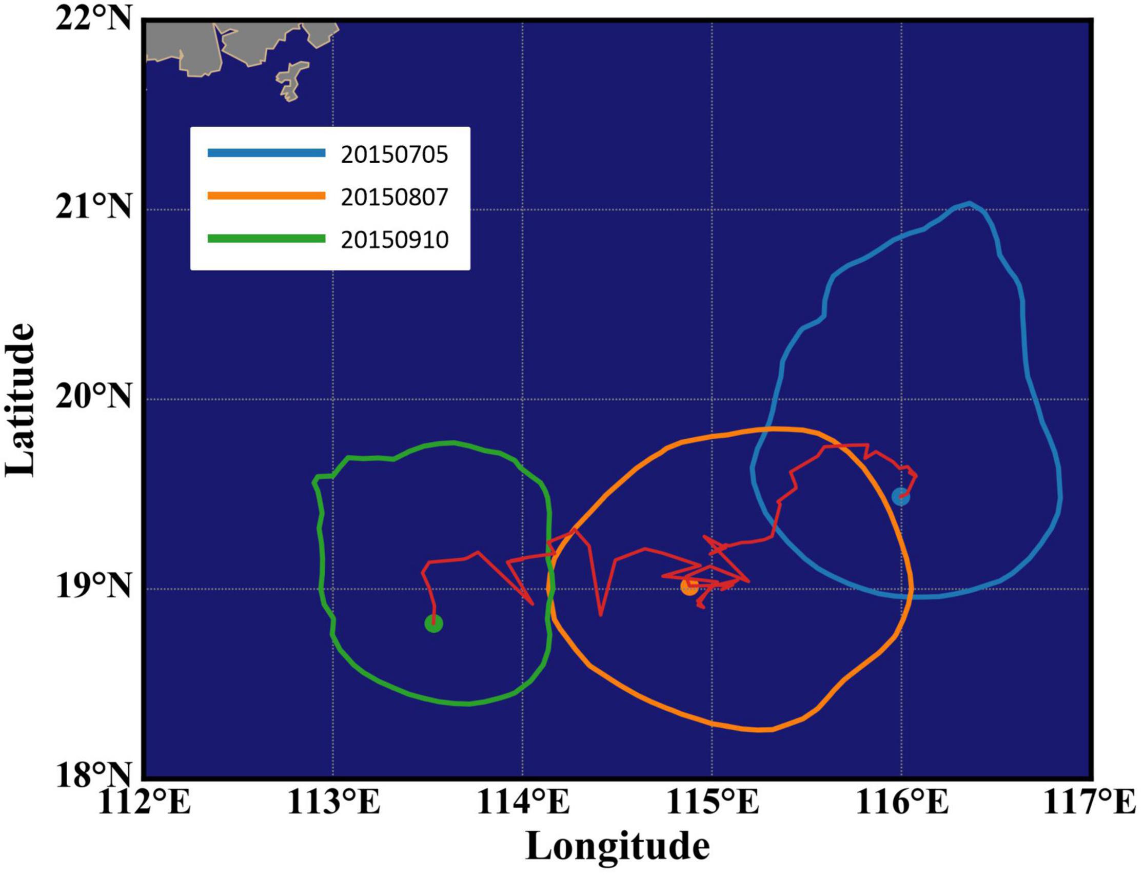
Figure 1. The trajectory of the target eddy (red line) and the eddy boundary on birth (20150705, blue line), death (20150910, green line), and intermediate days (20150807, orange line).

Adaptive Network Design Under Eddy Normalization

In the field observation of ocean mesoscale eddies, glider is widely used with its high maneuverability and flexibility. However, due to limited sailing speed and battery life (Paley et al., 2008), it is still impossible for us to continuously obtain observation data at each position inside an eddy. How to reasonably plan the glider path, select the most effective observation points, and ensure that the most valuable data can be obtained are the critical problems addressed in this paper.

The optimal interpolation method is used to estimate the optimal value (e.g., temperature and salinity) at grid points inside eddy (Marchuk, 1974). The implementation of this method relies on the background field X^b in the observation area and the observed value X^o at the observation points. In the simulation experiment, multi-day averages are used as background field. The difference D between the observed value and the background value at the observation point is:

$D=X^o-H{X}^b(1)$

where the symbol H represents the observation matrix, which can realize the mapping from regular grid to measurement location. The error covariance matrix P^b of background field at all grid points is obtained through the Gaussian function of the distance between two points:

$P^b(x_i,y_i,x_j,y_j)=\exp \left(-\left(\frac{{\left(x_i-x_j\right)}^2}{L_x^2}+\frac{{\left(y_i-y_j\right)}^2}{L_y^2}\right)\right)(2)$

where x and y are the coordinates of different grid points, respectively; L is the correlation length parameter, which is determined by the scale of ocean phenomenon we observed. L_x = L_y = 0.2 are selected in the simulation experiment, which is a suitable choice for L varying from 0 to 1 after several experiments. Its unit is in degrees, because the units of input coordinates x and y are in degrees. The diagonal element of the error covariance matrix P^b represents the variance of the error. According to the principle of minimum mean square error, the Kalman gain matrix K is defined as:

$K=P^b{H}^T{\left(H{P}^b{H}^T+R\right)}^{-1}(3)$

where R is the observation error covariance matrix. HP^bH^T represents the error covariance matrix between different observation points, P^bH^T means the error covariance matrix between grid points and observation points, and the Kalman gain matrix K actually represents different weights of the prior knowledge (that is, the background field). The larger K is, the more estimated value attaches attention to the feedback of observed value. Conversely, the smaller K is, the closer estimated value is to the prior knowledge. Formula (4) and (5) are used to calculate the posterior estimated value X^a and its error covariance matrix P^a, respectively.

$X^a=X^b+KD(4)$

$P^a=P^b-KH{P}^b(5)$

The error covariance matrix P^a is a measure of the reliability of the field estimation, whose diagonal entries represent the variance of estimated value at grid points (Alvarez and Mourre, 2012; Ferri et al., 2015). Therefore, it’s better to select observation points with smaller trace of P^a. In other word, the cost function of this optimization problem is,

$J=\underset{(x,y)}{\text{argmin}}\left(\frac{tr\left(P^a\right)}{N}\right)=\underset{(x,y)}{\text{argmin}}\left(\frac{tr\left(P^b-KH{P}^b\right)}{N}\right),(x,y)\in \mathrm{\Omega }(6)$

where Ω represents all grid points inside eddy, and N is the number of grid points.

It is worth mentioning that the cost function J is only related to the error covariance matrix P^a, and the solution of P^a only needs the location of observation point, while the value of observation point is not necessary. This feature allows the above calculation to be completed and scheme to be planned before the implementation of observation mission, which makes it possible for the algorithm to be applied in the field observation of ocean eddies.

In order to reduce the complexity of the simulation experiment, the target eddy is normalized into standard circle according to the information of radius and boundary (Ma et al., 2019b,2020). At the same time, the position of glider is also normalized according to the radius of eddy and the distance from glider to the eddy center. The distance from glider to the eddy center is D_g, the azimuth angle is, and the radius of the target eddy is D_r, then the position (x, y ) of glider in the standard circle can be calculated by:

$x=\frac{D_g}{D_r}*\cos \mathrm{\alpha }(7)$

$y=\frac{D_g}{D_r}*\sin \mathrm{\alpha }(8)$

In this paper, the Particle Swarm Optimization algorithm (PSO) (Kennedy and Eberhart, 1995) is used to select the optimal observation points corresponding to the minimum value of the cost function. It is a solution method with the characteristic of fast convergence speed, resulting in obtaining the global optimal solution easily.

We take the heading angle of glider as the independent variable in the PSO. When the heading angle of the glider is known to be θ, the coordinates of the observation point can be calculated by:

$x_i=x_0+dis*\text{cos}(\mathrm{\theta })(9)$

$y_i=y_0+dis*sin(\mathrm{\theta })(10)$

(x₀, y₀) is the starting position of glider, which is set as the eddy center in the first period of the simulation experiment. Considering the diving depth and pitch angle of glider, the predetermined distance between two adjacent observation points is set as 5 km.

The optimal heading angles θ are calculated by multiple iterations of Formula (11) and (12).

$\mathrm{△}\mathrm{\theta }\left(t+1\right)=w\mathrm{△}\mathrm{\theta }\left(t\right)+c_1{r}_1\left({\mathrm{\theta }}_i\left(t\right)-\mathrm{\theta }\left(t\right)\right)+c_2{r}_2\left({\mathrm{\theta }}_p\left(t\right)-\mathrm{\theta }\left(t\right)\right)(11)$

$\mathrm{\theta }\left(t+1\right)=\mathrm{\theta }\left(t\right)+\mathrm{△}\mathrm{\theta }\left(t+1\right)(12)$

where w is called inertia weight, c₁ and c₂ are learning factors, r₁ and r₂ are variation factors. θ_i and θ_p are the best heading angle of particle individual and particle population. In each iteration, the inertia weight w is determined by the typical linear decline strategy. Its value can be calculated according to the following formula:

$w=w_{max}-\frac{step}{maxStep}\left(w_{max}-w_{min}\right)(13)$

We set w_min = 0.1, w_max = 0.9 and maxStep = 100 in the simulation experiment. The linear decline strategy of the inertia weight has the following characteristics: the inertia weight w is larger in the initial iteration, thus the algorithm has a good global search ability to achieve fast convergence. With the increase of iterations, the inertia weight w becomes smaller, which strengthens the local search ability of the algorithm and makes it easier to find the optimal result.

The learning factor c₁ and c₂ is usually selected as two equal values within the range of 0∼4. We set c₁ = c₂ = 1.4961. The random function are used to generate r₁ and r₂ randomly in the range of 0∼1 in the simulation experiment. The detailed calculation process can be found in Appendix.

Heading Angle Correction Algorithm

The underwater movement of glider is determined by the actual ocean current and the gliding speed, in which the gliding speed is determined by the pitch angle (Paley et al., 2008). An adaptive heading angle correction algorithm is proposed to counteract the disturbance of ocean current on the motion direction of glider. The algorithm calculates the velocity and direction of ocean current in the last period through the deviation between the actual and predicted arrival position of glider. In the latter period, the new heading angle is calculated to guarantee that glider will move along the predetermined path and reach the target observation point more accurately.

This algorithm includes lots of important parameters. Their symbols and meanings are illustrated in Table 1. In the implementation of this algorithm, we regard a daily observation of glider as a task, in which a number of observation points are included. The heading angle of glider will be updated by the algorithm at each observation point. Figure 2 draws the process of heading angle correction after glider emerges from sea surface.

TABLE 1

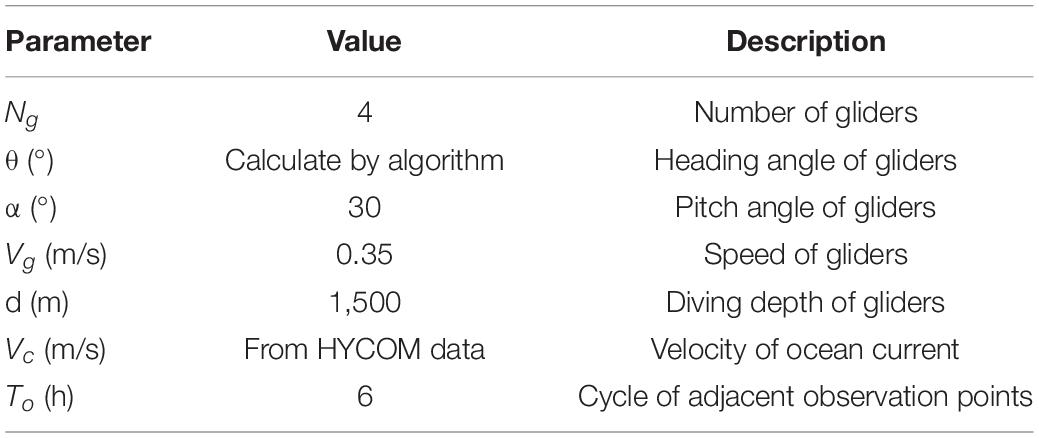
Table 1. Several parameters of gliders were set in the simulation experiment.

FIGURE 2

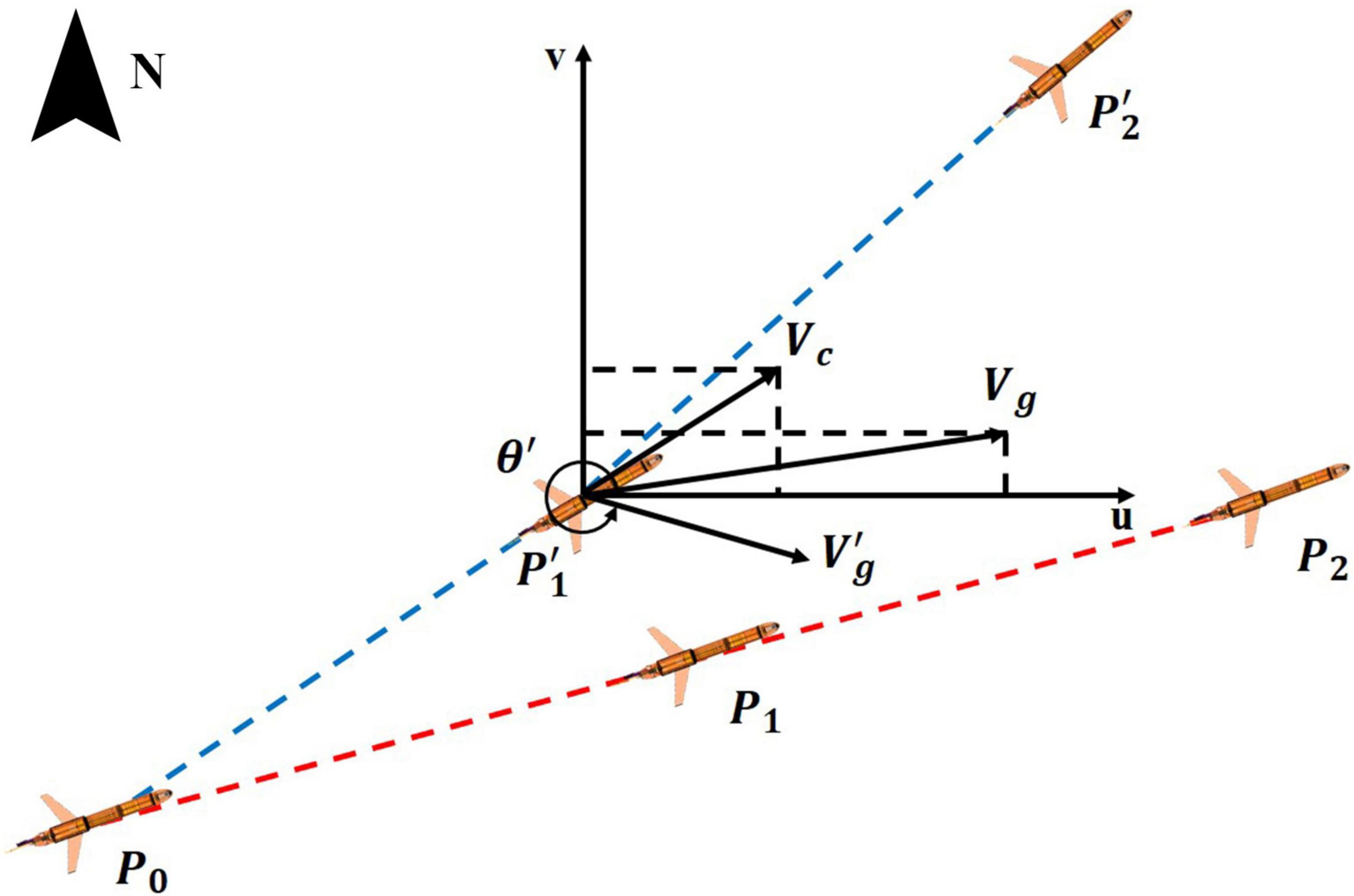
Figure 2. Diagram presents the process of heading angle correction at surface point. The red dotted line represents the predetermined route, and the blue dotted line represents the actual trajectory.

Glider starts from the initial point P₀, and we expect glider will arrive at the first observation point P₁ after T_o time. However, due to the influence of ocean current, the actual observation position is $P_1^{\prime }$. The ocean current V_c in the last period is calculated by:

$V_c=\frac{P_1-P_1^{\prime }}{T_o}(14)$

Combining the calculated ocean current V_c and the glider velocity V_g at the direction toward the target point, the new heading angle θ′ and the glider velocity $V_g^{\prime }$ at the direction of this new heading angle can be calculated by:

${\mathrm{\theta }}^{\prime }={\tan }^{-1}\left(\frac{{\left(V_g\right)}_y-{\left(V_c\right)}_y}{{\left(V_g\right)}_x-{\left(V_c\right)}_x}\right)(15)$

$V_g^{\prime }=V_g\text{[}\cos \left({\mathrm{\theta }}^{\prime }\right),\sin \left({\mathrm{\theta }}^{\prime }\right)](16)$

If glider does not correct heading angle at this observation point, the next observation point may be $P_2^{\prime }$ after 2T_o time. As a result, the deviation of the glider’s position from the target observation point will become much larger (Figure 2). On the contrary, if the heading angle is recalculated by the algorithm, the observation point P₂ will be back near the predetermined path in the next period. Its position can be calculated using the ocean current $V_c^{\prime }$ in the next period from HYCOM data.

$P_2=P_1^{\prime }+\left(V_g^{\prime }+V_c^{\prime }\right)T_s(17)$

In order to verify the effectiveness of the adaptive heading angle correction algorithm, a field experiment was conducted in the SCS. The glider used in the field experiment is a new type of glider developed by the Ocean University of China combing with several other research institutes, named as “SmartFloat.” Figure 3 shows the sailing trajectory of the glider we used in the experiment. The yellow solid line is the planned observation path, the red dotted line represents the actual trajectory, and the green circles are the observation points. The blue arrows are the direction of heading angles calculated by this algorithm. What can be find from the trajectory is that the initial motion direction of the glider deviates from the expected direction due to the influence of ocean current. If the glider continues to move in accordance with the initial heading angle, its observation point is likely to be farther away from the target observation point after several periods. However, after the heading angle of each observation point is corrected by the algorithm, the final trajectory is arc-shaped and the actual location of glider is not far from the target point. Therefore, this experiment verified that the algorithm can ensure glider to sample data near the target point.

FIGURE 3

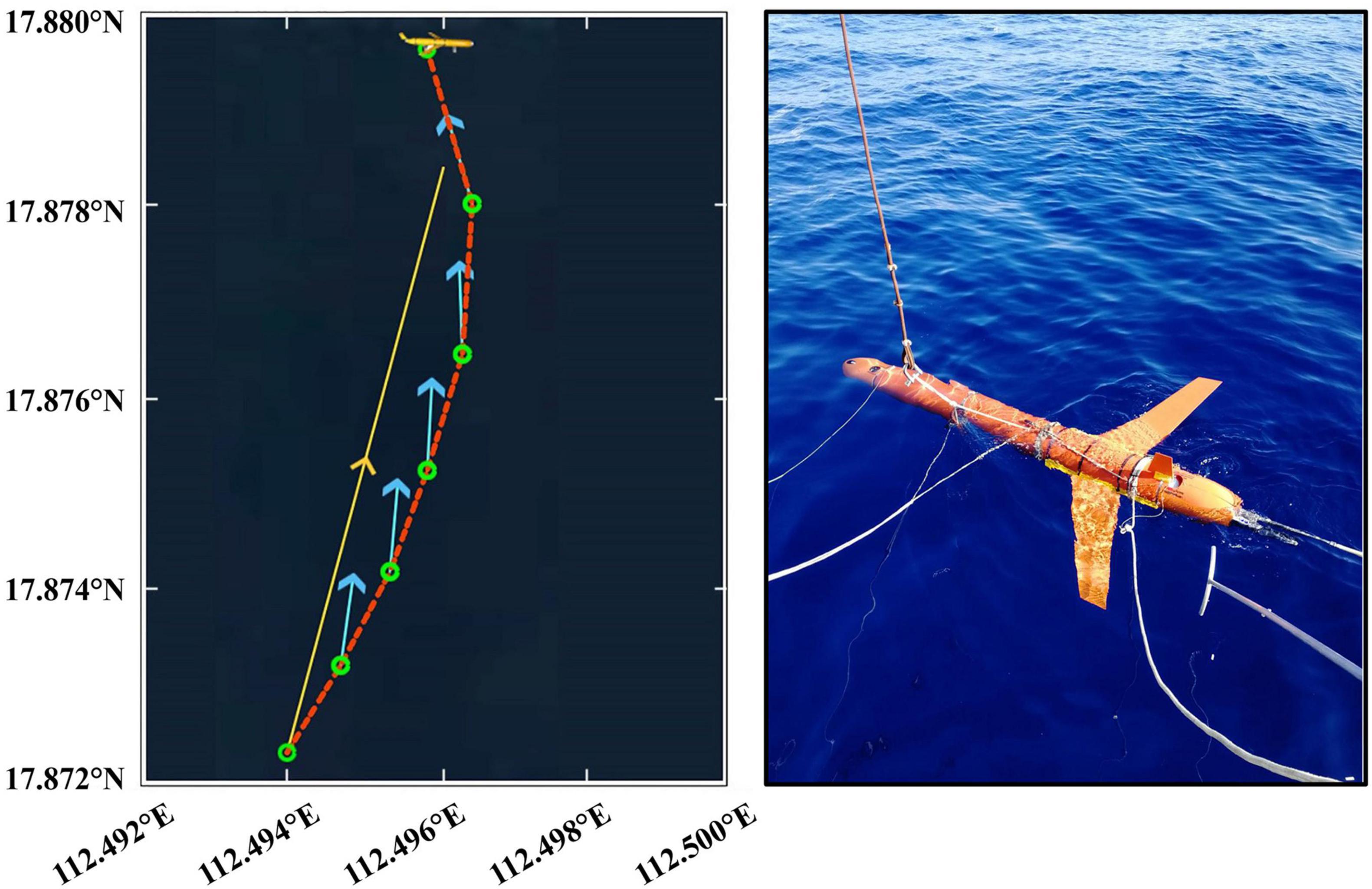
Figure 3. Left shows the glider trajectory in the field experiment and right shows the glider used in this experiment. The solid yellow line is the planned route, the dotted red line is the actual trajectory, the green circles represent the location of each surface point, and the blue arrows are the heading angles calculated by the algorithm.

Simulation Experiment and Results

Experiment Design

Based on the dataset of eddy identification and tracking and the realization of the adaptive heading angle correction algorithm, we design a network tracking simulation experiment of multiple gliders for eddy observation in the SCS. The flow diagram of the simulation experiment is shown in Figure 4.

FIGURE 4

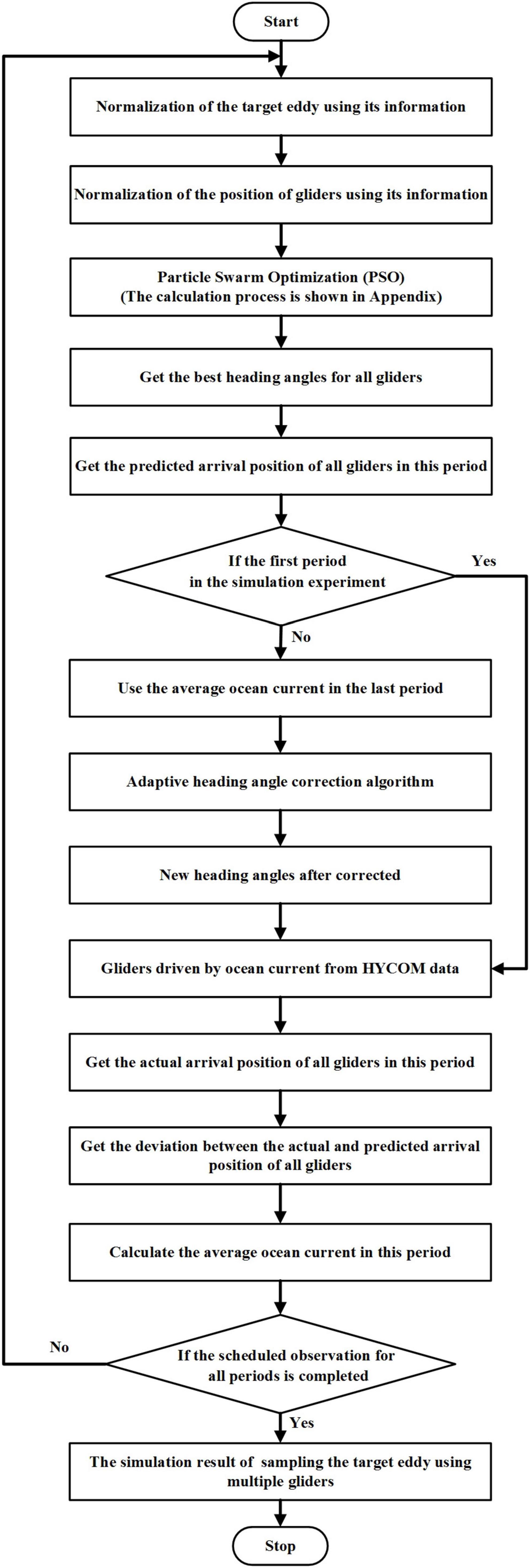
Figure 4. The flow chart of the simulation experiment.

An anticyclonic eddy located between the Hainan island and the Luzon strait was selected as the target eddy in the simulation experiment. Its trajectory was marked with a solid red line in Figure 1. Taking the eddy center as the starting observation point, gliders were used to track the target eddy for 20 days from July 5 to 24, 2015. The detailed parameters set in this simulation experiment can be referred to Table 1.

The process of four gliders sampling the target eddy is shown in Figure 5. Color in the figure represents the temperature anomaly of 80 m depth in the target eddy region. The length and direction of black arrows represent the direction and intensity of ocean current, respectively, while the red solid line represents the boundary of target eddy. The trajectories of four gliders are represented by solid lines in different colors. The result of the 20-day observation (Figure 5) shows that gliders’ trajectories gradually covered most areas inside the eddy with time going by.

FIGURE 5

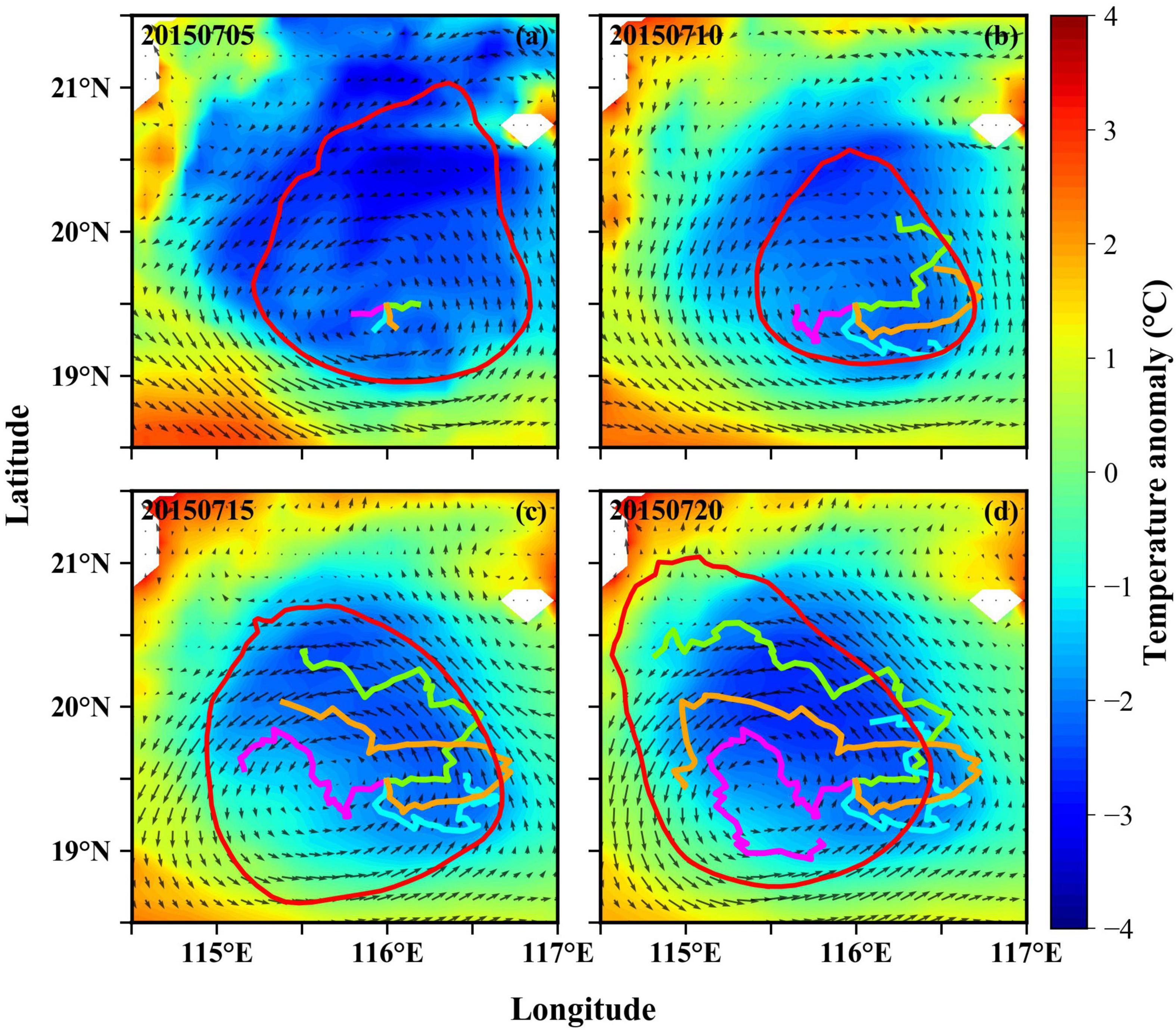
Figure 5. (a–d) Show the network observation results of four gliders sampling the target eddy from July 5 to July 20, 2015. The bottom color represents the temperature anomaly, the red solid line is the eddy boundary, and different color solid lines inside the target eddy represent the motion trajectory of each glider.

In Figure 5b, when two gliders (marked by lawn green and orange, respectively) reached the right boundary of the eddy on July 10, 2015, they both turned to the left and then moved northwest to those areas within the eddy that had not yet been observed. When approached the southern boundary of the eddy, the other two gliders (represented by fuchsia and cyan) turned left and right, respectively, for the next period of observation, both of them had a tendency of moving northward. This phenomenon shows that when gliders approached or crossed the eddy boundary, the adaptive network design algorithm proposed in this article was able to plan a reasonable trajectory and calculate the position of target point need to be observed in the next cycle. As a result, the glider was driven to the unobserved area inside the target eddy, and an effective observation network was designed. On July 20, 2015, when two gliders (represented by lawn green and orange) approached the left boundary of the target eddy (Figure 5d), they changed their sailing directions and moved toward the interior of the eddy to conduct the following observation, which confirmed the above conclusion again.

After several days of continuous observation, four gliders were able to track the target eddy to the southwest and remained inside the eddy. In order to show the relative position of observation points more clearly, we normalized the target eddy into a standard circle. Figure 6 shows the relative position of observation points inside the standardized eddy at different times.

FIGURE 6

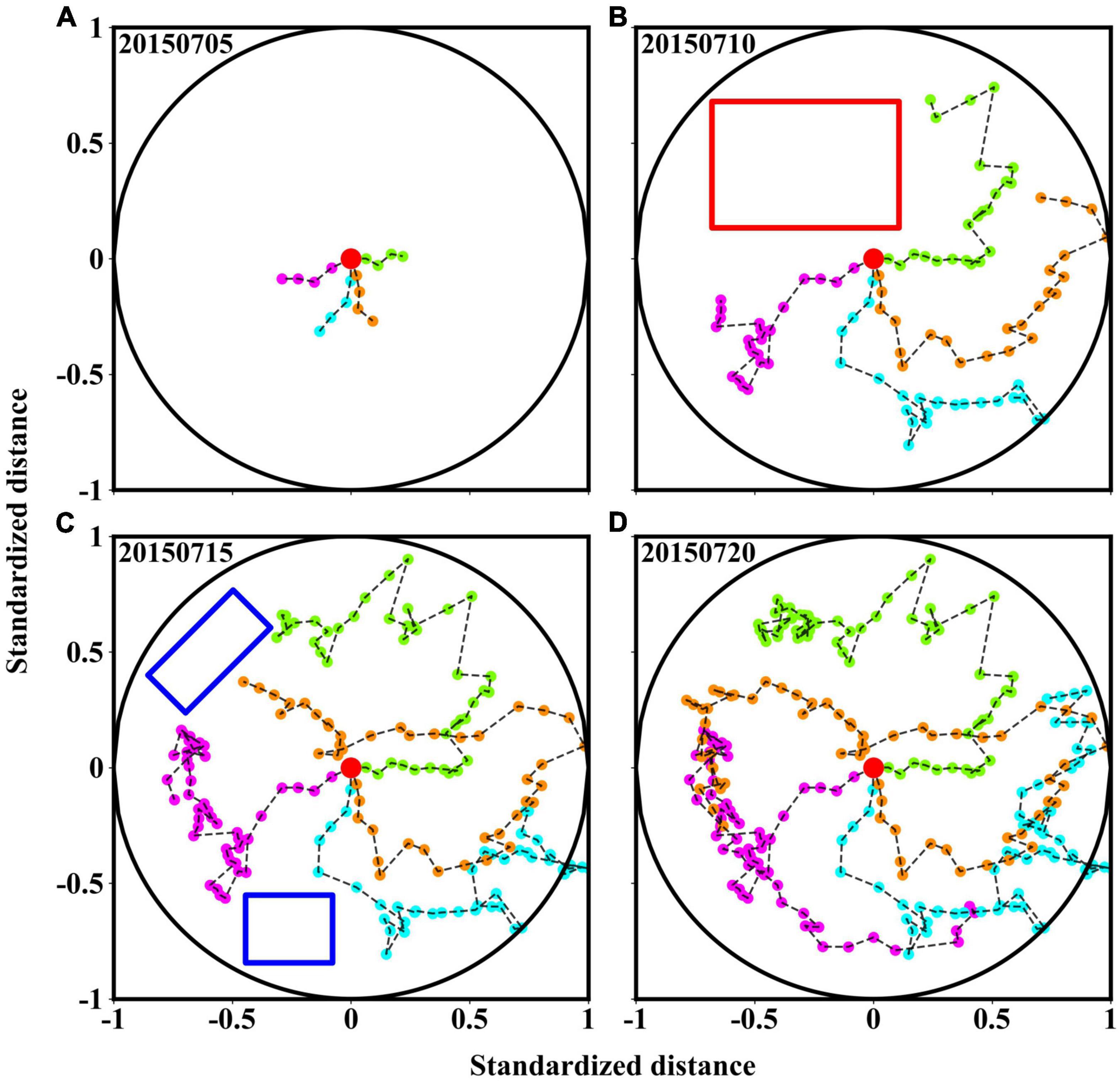
Figure 6. (A–D) Show the position of gliders within the standard circle from July 5 to July 20, 2015, which are indicated by the different color dots. Red and blue rectangles represent areas that lack sufficient observation points.

Due to the observation time and the speed of gliders, these failed to achieve uniform observation inside eddy on July 10, 2015 (Figure 6B). Almost a quarter in the northwest region of the eddy were not observed (shown by the red rectangle). Combined with Figure 5c, we found that two gliders (represented by lawn green and orange) focused on sampling within the red rectangle in the following 5 days, indicating that the algorithm selected the optimal observation points near the area. In addition, looking at the blue box in Figure 6C, we found that there were still some blank areas in the northwest and southwest near the boundary on July 15, 2015. Under the planning of the algorithm, some observation points were added in this area on July 20, 2015. The distribution variation of observation points in different periods shows the effectiveness of the algorithm in multiple gliders networking. With the increase of observation time, gliders gradually realized the observation in all directions within the target eddy.

Data Interpolation

The optimal interpolation method is used to interpolate the single-point observation data into continuous grid data (L’Hévéder et al., 2013; Amores et al., 2018). The optimal interpolation method is a linear interpolation method with the minimum mean square error (Marchuk, 1974). The principle of this method is to search multiple observation points participating in estimating the values of grid points based on the given spatial scale. Then, the different weight of each observation point could be calculated through the covariance matrix between grid points and observation points. Finally, the optimal values of grid points could be estimated according to the values and corresponding weights of these observation points.

Figure 7 shows the variation of the residual errors between the true value from HYCOM data and the estimated value from OI interpolation from July 5 to July 20, 2015. In the initial observation stage, the areas with low residual errors are distributed near the starting point (eddy center), while most other areas have large residual errors due to the lack of enough observation points. The residual errors inside the eddy decreased continuously with the increase of observation time, and decreased to a lower level on July 20, 2015. The variation of the pattern of the residual errors inside the eddy is similar to that of the trajectory of gliders, indicating that they are closely related.

FIGURE 7

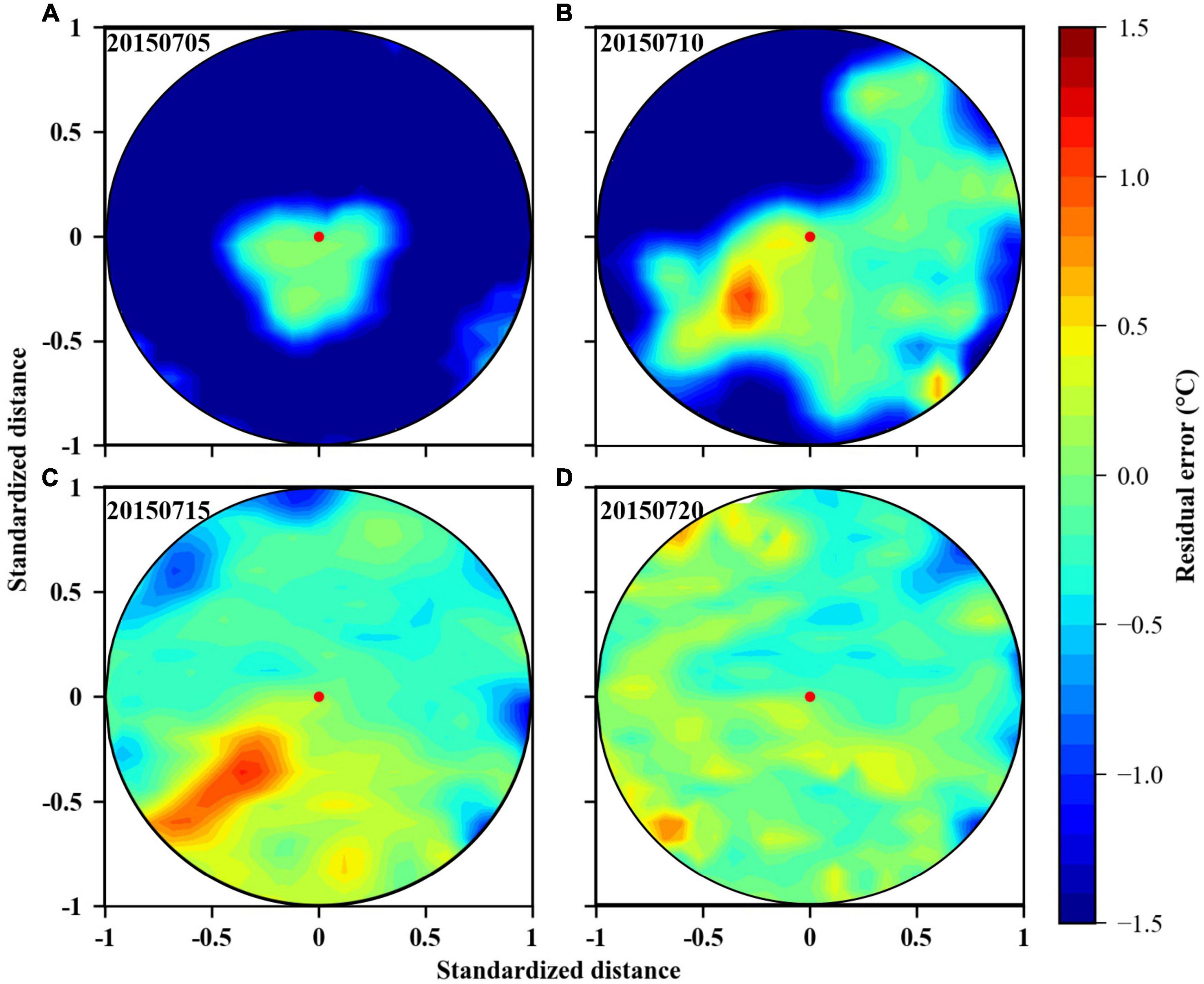
Figure 7. (A–D) Show the distribution of the residual errors inside the standard circle from July 5 to July 20, 2015.

Experiments With Different Parameters

The simulator provides multiple parameter inputs of gliders with different number (including 2, 4, and 6 gliders) and speed (including 0.32, 0.35, and 0.38 m/s speed). Figures 8, 9 show the simulation results on July 24, 2015. Among them, Figure 8 shows the observation results of different number of gliders following the eddy at the speed of 0.35 m/s for 20 days. While in Figure 9, the observation results of four gliders following eddy at different speed of gliders for 20 days are plotted. These two figures include the final trajectory of gliders, the normalized position of observation points on July 24, 2015.

FIGURE 8

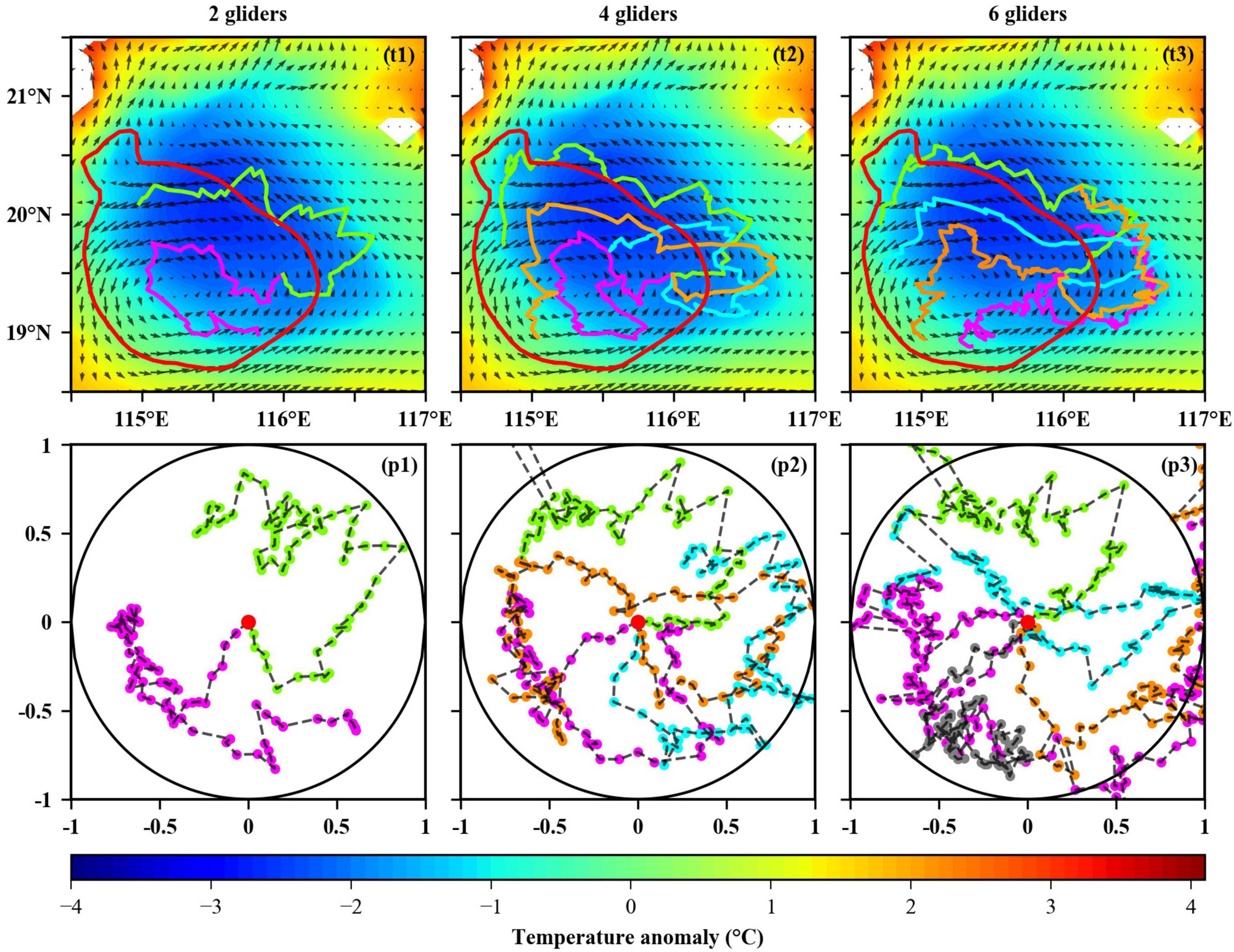
Figure 8. The results of 2, 4, and 6 gliders used to track the target eddy on July 24, 2015. The first column is the trajectory of gliders, the second column is the normalized position of gliders.

FIGURE 9

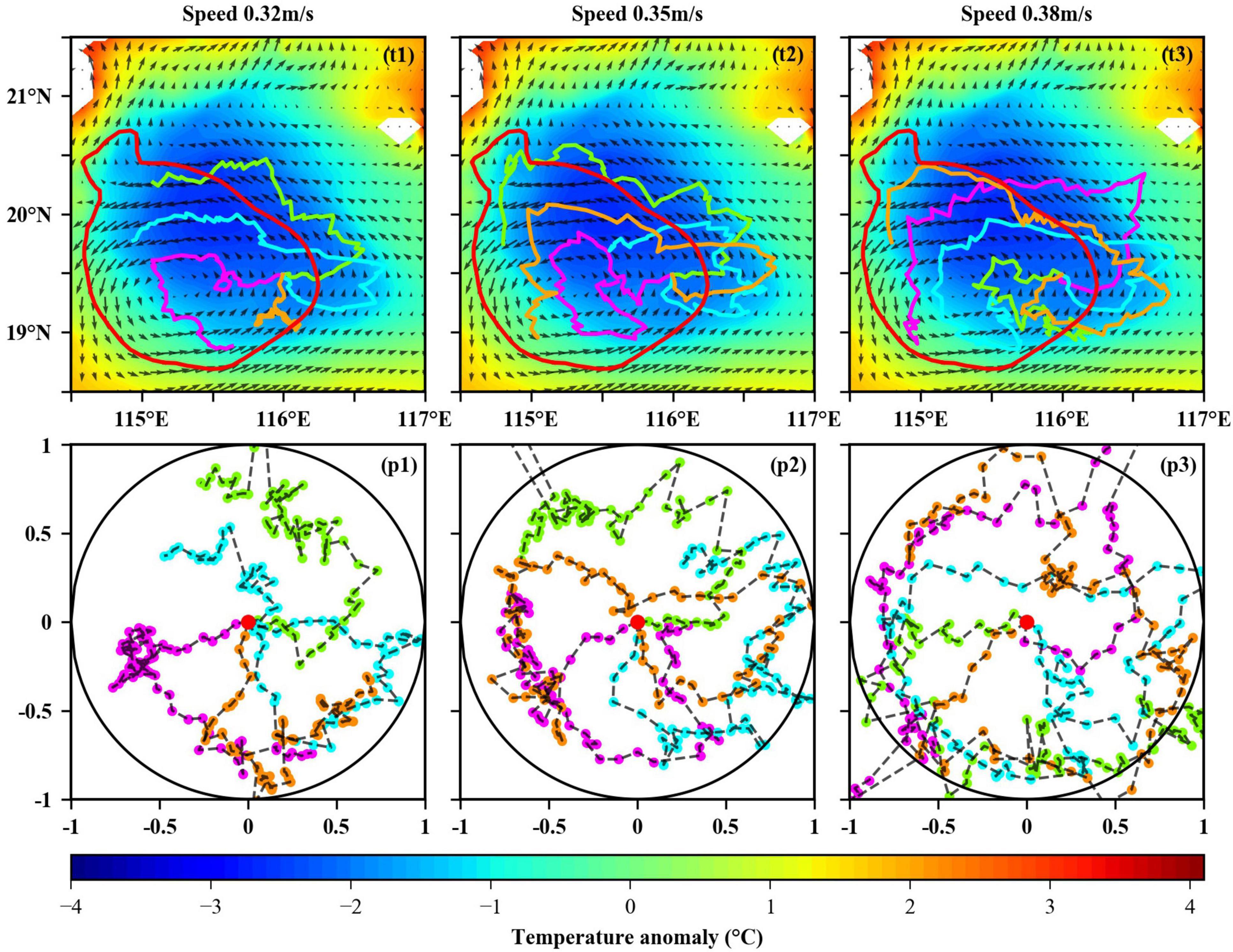
Figure 9. The results of gliders at the speed of 0.32 m/s, 0.35 m/s, and 0.38 m/s used to track the target eddy on July 24, 2015. Similarly, the first column is the trajectory of gliders, the second column is the normalized position of gliders.

Discussion

Comparison With “Cross Sampling”

At present, the main means for mesoscale eddy observation is focused on using one or multiple gliders to sample along cross-shaped route inside the eddy, or in accordance with the pre-planned straight route to form gridline trajectory (L’Hévéder et al., 2013). This traditional observation scheme is easy to design and not strict in the setting of glider’s parameters, but the quality of observation data and the synthetic result of characteristic information cannot be guaranteed. Note that the traditional observation scheme which samples along cross-shaped route inside the eddy is named “Cross Sampling” in this article. The sampling scheme planned by the algorithm we proposed is named “Optimal Sampling.” In this part, “Cross Sampling” method and “Optimal Sampling” method are systematically compared and discussed from the observation results of different simulation experiments to the interpolation results of data observed inside eddy.

A simulation experiment using “Cross Sampling” method to track the same target eddy was conducted. In the initial stage, all gliders started from the eddy center and moved in the direction of initial heading angles which are uniformly distributed in different directions. When gliders reached or went beyond the eddy boundary, their movement direction would change to the eddy center in place to ensure that these gliders would sample inside eddy as much as possible. If gliders returned to the nearby regions of the eddy center, they would change their directions and continue to move in the direction of their initial heading angles. As for how to judge whether gliders reached the nearby regions of the eddy center or not, the distance threshold was set as 1 km in this simulation experiment. In other words, we believe that glider has reached the eddy center if the distance between the observation position of glider and the eddy center is less than 1 km. Figure 10a shows the 20-day trajectories of four gliders following the eddy at the speed of 0.35 m/s using the “Cross Sampling” method from July 5 to 24, 2015. The final trajectories are roughly the superposition of multiple cross-shaped, consistent with the distribution of observation points in the standard circle shown in Figure 10b.

FIGURE 10

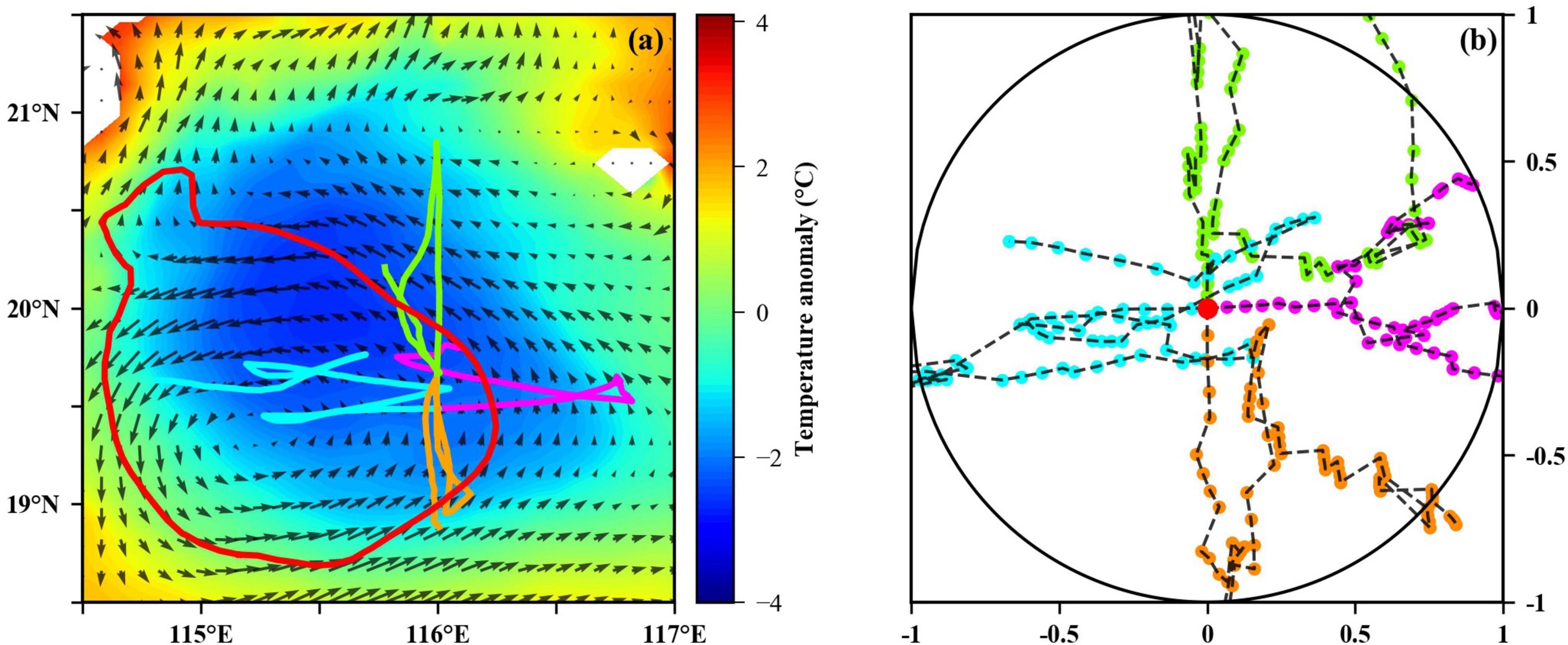
Figure 10. The network observation result of four gliders sampling the target eddy by the traditional “Cross Sampling” method on July 24, 2015. (a) Is the trajectory of each glider, (b) is the normalized position of gliders within the standard circle.

The same data interpolation method (Optimal Interpolation) is used to interpolate observation data obtained in the “Cross Sampling” simulation experiment. Figure 11 shows the true value of temperature anomaly in HYCOM data, the estimated value of temperature anomaly from optimal interpolation, and the residual errors between true value and estimated value on July 24, 2015 in both “Optimal Sampling” and “Cross Sampling” simulation experiment. It can be seen that the estimated value in “Optimal Sampling” (Figure 11B) was similar to the true value of HYCOM data (Figure 11A), showing that the maximum temperature anomaly tilted to northeast. The RMS (Root Mean Square) of residual errors was 0.31°C.

FIGURE 11

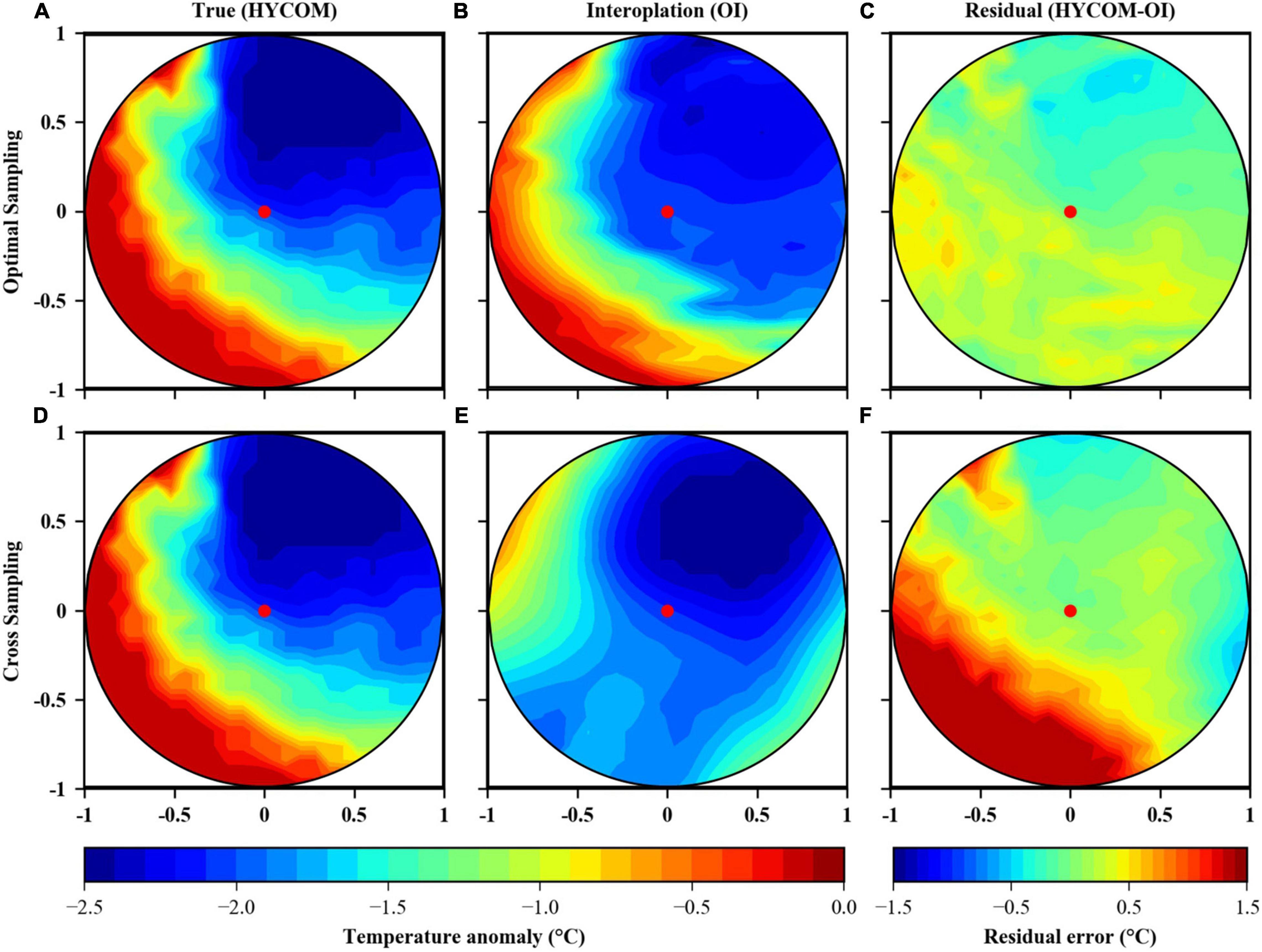
Figure 11. Comparison of temperature anomaly inside the target eddy on July 24, 2015. The first row is the synthetic results of the “Optimal Sampling,” the second row is the synthetic results of the “Cross Sampling”. (A,D) Are the true value of HYCOM data, (B,E) are the estimated value after data interpolation, (C,F) are the residual errors between the estimated value and the true value.

The pattern of the estimated value in “Cross Sampling” also roughly reflects the characteristic that the maximum temperature anomaly tilted to the direction of northeast. Due to the limitations of this observation scheme, there were not enough observation points in the southwest of the target eddy, in which the estimation of temperature anomaly can only rely on observation data in the west and south directions. Compared with the true value of HYCOM data (Figure 11D), the interpolation result (Figure 11E) didn’t reflect the warming trend of temperature anomaly in the southwest direction, resulting in the increase of residual errors in this direction (Figure 11F). The RMS of residual errors within the target eddy was 0.68°C, which is larger than that of the “Optimal Sampling” method. The inaccurate estimation demonstrated the superiority of observation scheme planned by the glider adaptive network design algorithm.

In addition, Figure 12 plots the average residual errors of two observation methods from July 5 to July 24, 2015. It can be concluded that residual error of the “Optimal sampling” method is always lower than that of the traditional “Cross Sampling” method during observation mission, which means that the final synthetic result is closer to the true value. These results indicate that the observation data obtained by the solution proposed in this paper are more valuable to describe the essential temperature characteristics of eddies.

FIGURE 12

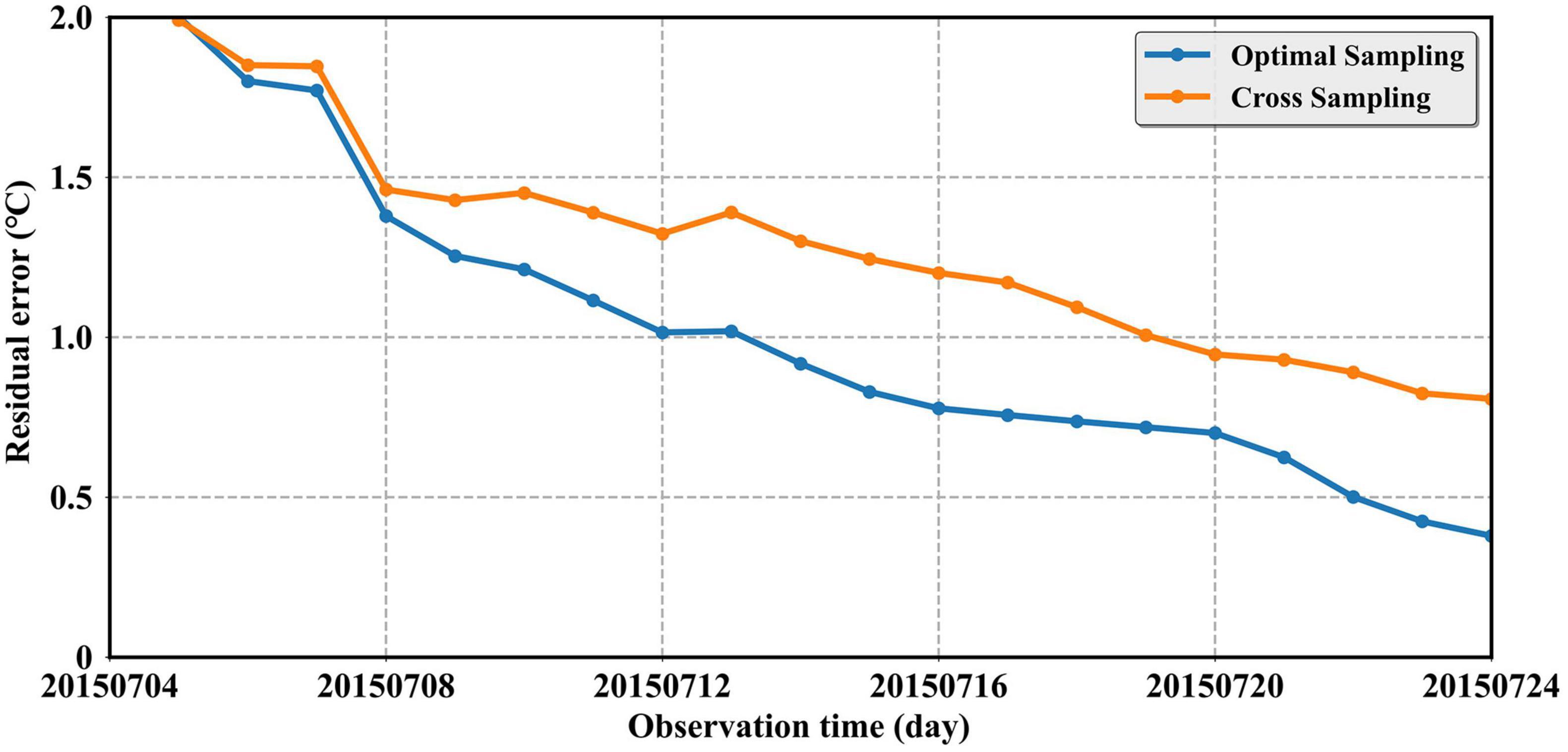
Figure 12. The curves of the average residual errors within the target eddy of two methods varying with the observation time from July 5 to July 24, 2015.

In order to increase the reliability of the conclusions, we selected another 200 eddies (including 100 anticyclonic eddies and 100 cyclonic eddies) from eddies dataset in 2015 for observation. The results of statistical experiments are shown in Table 2. The tracking results of more eddies verify again that the residual errors in the “Optimal sampling” scheme is always smaller than that of the “Cross Sampling” method, and the observation accuracy is improved by about 0.2°C. For different types of eddies, there is no obvious difference between the residual errors of anticyclonic eddies and cyclonic eddies.

TABLE 2

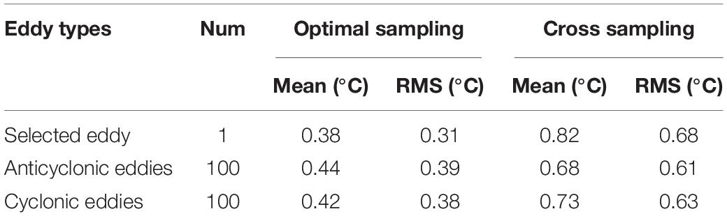
Table 2. Statistical results of the residual errors in simulation experiments.

Underlying Assumptions and Biases

There are still many differences between the design of simulation experiment and the condition of field observation. This algorithm can drive gliders to realize the tracking observation of the target eddy based on the following assumptions. Firstly, the input of the algorithm needs the information of the target eddy, such as the daily eddy boundary. In the simulation experiment, we can use the previous eddy identification and tracking data, which cannot be obtained in the field observation. Therefore, if we want to apply this algorithm to field observation and solve the input problem of this algorithm, we can combine the eddy prediction technology to realize the prediction of a variety of eddy properties, including the lifetime, radius, moving direction and so on (Ma et al., 2019a). With the development of deep learning, this technology has been in-depth studied and gradually mature. It should be mentioned that numerical models can also be used as forecast to get eddies. Besides, we can use the quasi-real-time processing data of satellite remote sensing combined with the efficient eddy identification and tracking technology to achieve the quasi-real-time acquisition of the target eddy information.

Secondly, the speed and pitch angle of gliders were set to a constant in the simulation experiment. But in the field observation, the speed and pitch angle will change continuously in the process of the dive and surface due to the influence of practical factors such as the change of the seawater density or the limitation of the angle control ability, which may cause the deviation between the observation point calculated by the formula and the actual observation point. Fortunately, the existence of this bias can be accepted. As long as gliders return the GPS coordinate position at the observation point, the algorithm can always calculate the optimal observation position of the next period according to the actual observation point of the glider, no matter how much the deviation is between the theoretical observation point and the actual observation point.

Thirdly, the ocean current calculated by the heading angle correction algorithm is a constant, which represents the average value of the ocean current in the last period. However, the ocean current at each point is different in actual observation, and the average value of the ocean current in the last period does not represent the value of the ocean current in the next period. Therefore, the heading angle calculated by the correction algorithm may be not the optimal heading angle needed to set in the next period, but it must be very close to the optimal value logically. Because the average value of the ocean current in the last period has the minimum interval in time and space from the real value of the present current.

Fourthly, the same weight is given to observations close or far in time when calculating the value of the cost function in the implementation of the algorithm, which is based on the hypothesis of stationarity of the eddy. The algorithm aims to cover the interior of the whole eddy and track the target eddy as far as possible during its lifecycle. If the characteristics of the eddy changes, or we are only interested in the characteristics at a certain point inside the eddy, the hypothesis is no longer valid and it may be better to sample several times in the same location to see the evolution of these characteristics. This situation will not invalidate the algorithm completely, but it may be a possible limitation of the current version. More improved versions that can handle complex field observation situations can be further developed on the basis of the current version.

Conclusion

An adaptive network design algorithm for multiple gliders sampling in mesoscale eddies observation is proposed in this paper. The algorithm designs the optimal observation scheme according to the information of the target eddy, and obtains more valuable observation data for data interpolation, so as to ensure the accuracy of synthetic results of the characteristic information inside eddy. Besides, considering the interference of ocean current on the motion direction of glider, a heading angle correction algorithm is proposed to calculate the velocity and direction of ocean current in real-time, resulting in getting the new heading angle which should be set in the next period. The effectiveness of this algorithm has been verified in the SCS field experiment.

Based on the realization of the adaptive network design algorithm and the analysis of the underwater motion of glider, we carried out several simulation experiments by using the dataset of eddy identification and tracking and the ocean current data from HYCOM. Results show that gliders can realize more comprehensive observation inside the target eddy with the increase of observation time, and its relative position are more uniformly distributed in the standardized circle. In addition, we used different number (2, 4, and 6) and speed (0.32, 0.35, and 0.38 m/s) of gliders in our simulation experiments, respectively.

The optimal interpolation method was used to interpolate observation data obtained by gliders into continuous grid data in the simulation experiments. The final interpolation results reflected that the maximum temperature anomaly was inclined to the northeast direction inside the target eddy. The RMS of residual errors between the estimated value of interpolation result and the true value of HYCOM data was 0.31°C. Interpolation results indicated that compared with the traditional “Cross Sampling” method which samples the target eddy along a fixed path, the observation data obtained by the “Optimal Sampling” method is more valuable to describe the essential temperature characteristics of eddies. It can be seen that the residual error of the “Optimal Sampling” is always smaller during the whole observation mission. Especially for those areas which cannot be observed due to the limitations of traditional “Cross Sampling” method, the algorithm proposed in this paper shows obvious advantages.

This means that if the adaptive network design algorithm for multiple gliders proposed in this paper can be applied to field observation of mesoscale eddies, lower cost but more valuable observation data will be obtained, which will strongly support the research and theory development of mesoscale eddies. In order to better facilitate the observation of mesoscale eddies, more field experiments are needed to verify the reliability of the algorithm, rather than simulation experiments.

Data Availability Statement

The original contributions presented in the study are included in the article/supplementary material, further inquiries can be directed to the corresponding author/s.

Author Contributions

ZG performed methodology, software, data processing, visualization, and wrote the original draft. GC contributed to conceptualization, investigation, and supervision. YS wrote and edited the manuscript. JZ contributed to the image visualization. CM performed validation and review. All authors contributed to the article and approved it for publication.

Funding

This research was jointly supported by the National Natural Science Foundation of China (Grant Nos. 41906155 and 42030406), the Key Research and Development Program of Shandong Province (Grant No. 2019GHZ023), and the National Key Scientific Instrument and Equipment Development Projects of National Natural Science Foundation of China (Grant No. 41527901).

Conflict of Interest

The authors declare that the research was conducted in the absence of any commercial or financial relationships that could be construed as a potential conflict of interest.

Publisher’s Note

All claims expressed in this article are solely those of the authors and do not necessarily represent those of their affiliated organizations, or those of the publisher, the editors and the reviewers. Any product that may be evaluated in this article, or claim that may be made by its manufacturer, is not guaranteed or endorsed by the publisher.

References

Alvarez, A., and Mourre, B. (2012). Optimum sampling designs for a glider–mooring observing network. J. Atmospheric Oceanic Technol. 29, 601–612. doi: 10.1175/jtech-d-11-00105.1

CrossRef Full Text | Google Scholar

Alvarez, A., Garau, B., and Caiti, A. (2007). “Combining networks of drifting profiling floats and gliders for adaptive sampling of the Ocean,” in Proceeding of the Paper Presented at the IEEE International Conference on Robotics and Automation, (Roma).

Google Scholar

Amores, A., Jordà, G., Arsouze, T., and Le Sommer, J. (2018). Up to what extent can we characterize ocean eddies using present-day gridded altimetric products? J. Geophys. Res. Oceans 123, 7220–7236. doi: 10.1029/2018jc014140

CrossRef Full Text | Google Scholar

Amores, A., Monserrat, S., Melnichenko, O., and Maximenko, N. (2017). On the shape of sea level anomaly signal on periphery of mesoscale ocean eddies. Geophys. Res. Lett. 44, 6926–6932. doi: 10.1002/2017gl073978

CrossRef Full Text | Google Scholar

Barceló-Llull, B., Pascual, A., Ruiz, S., Escudier, R., Torner, M., and Tintoré, J. (2019). Temporal and spatial hydrodynamic variability in the mallorca channel (western mediterranean sea) from 8 years of underwater glider data. J. Geophys. Res. Oceans 124, 2769–2786. doi: 10.1029/2018JC014636

CrossRef Full Text | Google Scholar

Bosse, A., Fer, I., Lilly, J. M., and Siland, H. (2019). Dynamical controls on the longevity of a non-linear vortex: the case of the lofoten basin eddy. Sci. Rep. 9, 1–13. doi: 10.1038/s41598-019-49599-8

PubMed Abstract | CrossRef Full Text | Google Scholar

Bosse, A., Testor, P., Mayot, N., Prieur, L., D’Ortenzio, F., Mortier, L., et al. (2017). A submesoscale coherent vortex in the ligurian sea: from dynamical barriers to biological implications. J. Geophys. Res. Oceans 122, 6196–6217. doi: 10.1002/2016JC012634

CrossRef Full Text | Google Scholar

Chaigneau, A., Le Texier, M., Eldin, G., Grados, C., and Pizarro, O. (2011). Vertical structure of mesoscale eddies in the eastern south pacific ocean: a composite analysis from altimetry and argo profiling floats. J. Geophys. Res. Oceans 116:134. doi: 10.1029/2011jc007134

CrossRef Full Text | Google Scholar

Chelton, D. B., Schlax, M. G., and Samelson, R. M. (2011). Global observations of nonlinear mesoscale eddies. Prog. Oceanogr. 91, 167–216. doi: 10.1016/j.pocean.2011.01.002

CrossRef Full Text | Google Scholar

Chelton, D. B., Schlax, M. G., Samelson, R. M., and de Szoeke, R. A. (2007). Global observations of large oceanic eddies. Geophys. Res. Lett. 34:30812. doi: 10.1029/2007gl030812

CrossRef Full Text | Google Scholar

Chen, G., Tang, J., Zhao, C., Wu, S., Yu, F., Ma, C., et al. (2019b). Concept design of the “guanlan” science mission: china’s novel contribution to space oceanography. Front. Mar. Sci. 6:194. doi: 10.3389/fmars.2019.00194

CrossRef Full Text | Google Scholar

Chen, G., Han, G., and Yang, X. (2019a). On the intrinsic shape of oceanic eddies derived from satellite altimetry. Remote Sensing Environ. 228, 75–89. doi: 10.1016/j.rse.2019.04.011

CrossRef Full Text | Google Scholar

Chen, G., Hou, Y., and Chu, X. (2011). Mesoscale eddies in the South China sea: mean properties, spatiotemporal variability, and impact on thermohaline structure. J. Geophys. Res. Oceans 116:716. doi: 10.1029/2010jc006716

CrossRef Full Text | Google Scholar

Cotroneo, Y., Aulicino, G., Ruiz, S., Pascual, A., Budillon, G., Fusco, G., et al. (2016). Glider and satellite high resolution monitoring of a mesoscale eddy in the algerian basin: effects on the mixed layer depth and biochemistry. J. Mar. Syst. 162, 73–88. doi: 10.1016/j.jmarsys.2015.12.004

CrossRef Full Text | Google Scholar

Curtin, T. B., Bellingham, J. G., Catipovic, J., and Webb, D. (1993). Autonomous oceanographic sampling networks. Oceanography 6, 86–94. doi: 10.5670/oceanog.1993.03

CrossRef Full Text | Google Scholar

Dong, C., McWilliams, J. C., Liu, Y., and Chen, D. (2014). Global heat and salt transports by eddy movement. Nat. Commun. 5:3294. doi: 10.1038/ncomms4294

PubMed Abstract | CrossRef Full Text | Google Scholar

Everett, J. D., Macdonald, H., Baird, M. E., Humphries, J., Roughan, M., and Suthers, I. M. (2015). Cyclonic entrainment of preconditioned shelf waters into a frontal eddy. J. Geophys. Res. Oceans 120, 677–691. doi: 10.1002/2014jc010301

CrossRef Full Text | Google Scholar

Ferri, G., Cococcioni, M., and Alvarez, A. (2015). Mission planning and decision support for underwater glider networks: a sampling on-demand approach. Sensors 16:28. doi: 10.3390/s16010028

PubMed Abstract | CrossRef Full Text | Google Scholar

Fu, L.-L., Chelton, D., Le Traon, P.-Y., and Morrow, R. (2010). Eddy dynamics from satellite altimetry. Oceanography 23, 14–25. doi: 10.5670/oceanog.2010.02

CrossRef Full Text | Google Scholar

Houpert, L., Inall, M. E., Dumont, E., Gary, S., Johnson, C., Porter, M., et al. (2018). Structure and transport of the north atlantic current in the eastern subpolar gyre from sustained glider observations. J. Geophys. Res. Oceans 123, 6019–6038. doi: 10.1029/2018jc014162

CrossRef Full Text | Google Scholar

Kennedy, J., and Eberhart, R. (1995). “Particle swarm optimization,” in Proceeding of the Paper Presented at the International Conference on Neural Networks, (Perth, WA).

Google Scholar

Le Traon, P. Y., Nadal, F., and Ducet, N. (1998). An improved mapping method of multisatellite altimeter data. J. Atmospheric Oceanic Technol. 15, 522–534. doi: 10.1175/1520-04261998015<0522:Aimmom<2.0.Co;2

CrossRef Full Text | Google Scholar

Leonard, N. E., Paley, D. A., Davis, R. E., Fratantoni, D. M., Lekien, F., and Zhang, F. (2010). Coordinated control of an underwater glider fleet in an adaptive ocean sampling field experiment in monterey bay. J. Field Robot. 27, 718–740. doi: 10.1002/rob.20366

CrossRef Full Text | Google Scholar

L’Hévéder, B., Mortier, L., Testor, P., and Lekien, F. (2013). A glider network design study for a synoptic view of the oceanic mesoscale variability. J. Atmospheric Oceanic Technol. 30, 1472–1493. doi: 10.1175/jtech-d-12-00053.1

CrossRef Full Text | Google Scholar

Li, S., Zhang, F., Wang, S., Wang, Y., and Yang, S. (2020). Constructing the three-dimensional structure of an anticyclonic eddy with the optimal configuration of an underwater glider network. Appl. Ocean Res. 95:101893. doi: 10.1016/j.apor.2019.101893

CrossRef Full Text | Google Scholar

Liu, Y., Chen, G., Sun, M., Liu, S., and Tian, F. (2016). A parallel SLA-based algorithm for global mesoscale eddy identification. J. Atmospheric Oceanic Technol. 33, 2743–2754. doi: 10.1175/jtech-d-16-0033.1

CrossRef Full Text | Google Scholar

Ma, C., Gao, Z., Li, S., Li, S., and Chen, G. (2020). An eddy-borne argo float measurement experiment in the south china sea. Ocean Dyn. 70, 1325–1338. doi: 10.1007/s10236-020-01402-3

CrossRef Full Text | Google Scholar

Ma, C., Li, S., Yang, Y., Yang, J., and Chen, G. (2019b). Extraction of revolving channels of drifters around mesoscale eddy centers based on spatiotemporal trajectory clustering. J. Atmospheric Oceanic Technol. 36, 1903–1916. doi: 10.1175/jtech-d-19-0007.1

CrossRef Full Text | Google Scholar

Ma, C., Li, S., Wang, A., Yang, J., and Chen, G. (2019a). Altimeter observation-based eddy nowcasting using an improved conv-LSTM network. Remote Sensing 11:783. doi: 10.3390/rs11070783

CrossRef Full Text | Google Scholar

Marchuk, G. I. (1974). Objective analysis of meteorological fields. Numerical Methods Weather Predict. 15, 242–258. doi: 10.1016/B978-0-12-470650-7.50013-X

CrossRef Full Text | Google Scholar

Martin, J. P., Lee, C. M., Eriksen, C. C., Ladd, C., and Kachel, N. B. (2009). Glider observations of kinematics in a gulf of alaska eddy. J. Geophys. Res. Oceans 114:231. doi: 10.1029/2008jc005231

CrossRef Full Text | Google Scholar

Morrow, R., Fu, L.-L., Ardhuin, F., Benkiran, M., Chapron, B., Cosme, E., et al. (2019). Global observations of fine-scale ocean surface topography with the surface water and ocean topography (SWOT) mission. Front. Mar. Sci. 6:232. doi: 10.3389/fmars.2019.00232

CrossRef Full Text | Google Scholar

Paley, D. A., Zhang, F., and Leonard, N. E. (2008). Cooperative control for ocean sampling: the glider coordinated control system. IEEE Trans. Control Syst. Technol. 16, 735–744. doi: 10.1109/tcst.2007.912238

CrossRef Full Text | Google Scholar

Pascual, A., Ruiz, S., Olita, A., Troupin, C., Claret, M., Casas, B., et al. (2017). A multiplatform experiment to unravel meso- and submesoscale processes in an intense front (AlborEx). Front. Mar. Sci. 4:39. doi: 10.3389/fmars.2017.00039

CrossRef Full Text | Google Scholar

Pelland, N. A., Bennett, J. S., Steinberg, J. M., and Eriksen, C. C. (2018). Automated glider tracking of a california undercurrent eddy using the extended kalman filter. J. Atmospheric Oceanic Technol. 35:126. doi: 10.1175/JTECH-D-18-0126.1

CrossRef Full Text | Google Scholar

Ramp, S. R., Davis, R. E., Leonard, N. E., Shulman, I., Chao, Y., Robinson, A. R., et al. (2009). Preparing to predict: the second autonomous ocean sampling network (AOSN-II) experiment in the monterey bay. Deep Sea Res. Part II Top. Stud. Oceanogr. 56, 68–86. doi: 10.1016/j.dsr2.2008.08.013

CrossRef Full Text | Google Scholar

Sun, M., Tian, F., Liu, Y., and Chen, G. (2017). An improved automatic algorithm for global eddy tracking using satellite altimeter data. Remote Sensing 9:206. doi: 10.3390/rs9030206

CrossRef Full Text | Google Scholar

Testor, P., Young, B. D., Rudnick, D., Glenn, S., and Wilson, D. (2019). Oceangliders: a component of the integrated goos. Front. Mar. Sci. 6:422. doi: 10.3389/fmars.2021.696100

CrossRef Full Text | Google Scholar

Tian, F., Wu, D., Yuan, L., and Chen, G. (2019). Impacts of the efficiencies of identification and tracking algorithms on the statistical properties of global mesoscale eddies using merged altimeter data. Int. J. Remote Sensing 41, 2835–2860. doi: 10.1080/01431161.2019.1694724

CrossRef Full Text | Google Scholar

Ubelmann, C., Cornuelle, B., and Fu, L.-L. (2016). Dynamic mapping of along-track ocean altimetry: method and performance from observing system simulation experiments. J. Atmospheric Oceanic Technol. 33, 1691–1699. doi: 10.1175/jtech-d-15-0163.1

CrossRef Full Text | Google Scholar

Yang, G., Yu, W., Yuan, Y., Zhao, X., Wang, F., Chen, G., et al. (2015). Characteristics, vertical structures, and heat/salt transports of mesoscale eddies in the southeastern tropical Indian Ocean. J. Geophys. Res. Oceans 120, 6733–6750. doi: 10.1002/2015jc011130

CrossRef Full Text | Google Scholar

Yu, L., Bosse, A., Fer, I., Orvik, K., Bruvik, E., Hessevik, I., et al. (2017). The lofoten basin eddy: three years of evolution as observed by seagliders. J. Geophys. Res. Oceans 122, 6814–6834. doi: 10.1002/2017JC012982

CrossRef Full Text | Google Scholar

Zamuda, A., Sosa, H., Daniel, J., and Adler, L. (2016). Constrained differential evolution optimization for underwater glider path planning in sub-mesoscale eddy sampling. Appl. Soft Comput. 42, 93–118. doi: 10.1016/j.asoc.2016.01.038

CrossRef Full Text | Google Scholar

Zhang, W., Xue, H., Chai, F., and Ni, Q. (2015). Dynamical processes within an anticyclonic eddy revealed from argo floats. Geophys. Res. Lett. 42, 2342–2350. doi: 10.1002/2015gl063120

CrossRef Full Text | Google Scholar

Zhang, Z., Tian, J., Qiu, B., Zhao, W., Chang, P., Wu, D., et al. (2016). Observed 3D structure, generation, and dissipation of oceanic mesoscale eddies in the south china sea. Sci. Rep. 6:24349. doi: 10.1038/srep24349

PubMed Abstract | CrossRef Full Text | Google Scholar

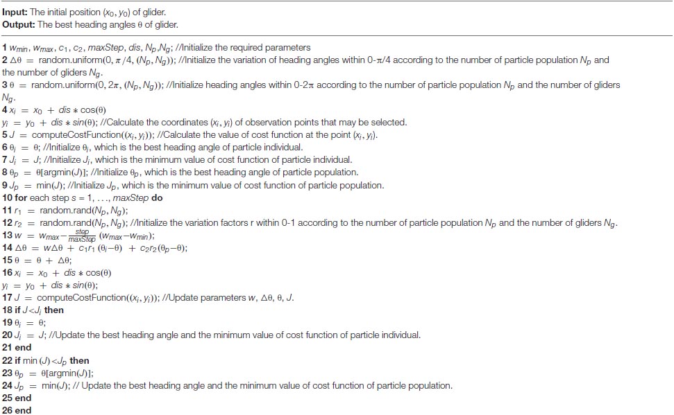
Appendix

The pseudocode for the calculation process of adaptive network design algorithm is as follows: