Quantifying Frontal-Surface Area of Woody Vegetation: A Crucial Parameter for Wave Attenuation

The last years, capacity of vegetation to reduce wave impact is receiving considerable attention. To predict wave attenuation processes within vegetation fields reliable estimates of vegetation parameters are needed. This proves to be difficult for woody vegetation as it consists of complex branch structures, characterized by varying branch densities, diameters and angles. State of the art physical and numerical models effectively use a single value for the diameter, b_v and density, N of vegetation, which is unrepresentative for complex vegetation, such as trees. Trees can be better described by the projected frontal-surface area, A_v. Hence, this work compares methods to quantify the A_v in space for a pollard willow forest, and determines suitability of these methods for predicting wave attenuation using a spectral wave model (SWAN). We use data from manual measurements and Terrestrial Laser Scans (TLS), to estimate the vertical distribution of A_v; and data from large-scale flume experiments performed on a willow forest to verify model sensitivity to A_v inferences. As a baseline for comparison, tree models that describe the structure of the trees in various degrees of complexity are compiled. The most realistic tree model is used to quantify potential errors in TLS and basic manual measurements of N and b_v. An initial comparison shows that the TLS data underestimates A_v, which indicates that conducting manual measurements is more suitable to quantify a homogeneous forest. We found that the TLS suffers from shadowing effects (i.e., blockage of laser beams) and we recommend to apply a correction factor to improve its measurements. Furthermore, we identified the impact that the different methods to determine A_v have on the estimation of wave attenuation using SWAN; in addition we verified the model results with data from large-scale flume experiments performed on the willow forest. The modeled sensitivity tests indicate large differences in wave attenuation and, consequently, a wide range (0.94–1.70) of bulk drag coefficients, ${\tilde{C}}_D$, for the various methods applied. This shows the variation of outcome between measuring methods and highlights the importance of stating the selected method for reliable frontal-surface area estimations, and consequently for reliable wave attenuation predictions.

1. Introduction

Current flood protection systems are under pressure due to climate change, in the form of more intense and frequent storms, heavier rainfalls, and accelerated sea level rise (Oppenheimer et al., 2019). Dikes will need to be made higher and stronger to keep up with changing climate, which will lead to increasing costs (Jonkman et al., 2013). Because of this, the interest in more cost-effective solutions has grown in recent years for both coasts and rivers. Using vegetation in front of dikes has attracted a lot of attention for its contribution to the flood safety, as it adapts to rising sea levels, promotes sedimentation and is able to attenuate incoming waves (van Wesenbeeck et al., 2013). Besides the flood safety benefits, these so called “eco-engineering solutions” or “hybrid flood defenses” provide several ecological benefits, such as increasing biodiversity by providing nursery habitat for fish and breeding areas for birds (Rog et al., 2017).

Many studies were conducted on wave attenuation (oscillatory flow) through vegetation fields, such as kelp (e.g., Mendez and Losada, 2004), salt marshes (e.g., Vuik, 2019) and mangroves (e.g., Mazda et al., 2006; Quartel et al., 2007). Two processes that lead to wave energy damping through vegetation are wave breaking and wave-vegetation interactions (Vo-Luong and Massel, 2008). Both vegetation characteristics (such as vegetation density, geometry and height) and hydrodynamic conditions (such as wave-current interactions, wave orbital velocity, and wave period (Hu et al., 2014) influence these processes. The hydrodynamics around one rigid cylinder and an array of rigid cylinders is relatively well understood under oscillatory flow, and is commonly used to mimic the presence of vegetation fields in physical and numerical models. These models use a simplified description of tree structures containing a single diameter and density of the branches. Woody vegetation, such as mangroves in tropical regions and willow trees in temperate regions, have complex structures (i.e., varying branch densities, diameters, and angles). These structures not only make it difficult to capture the hydrodynamics, but also the vegetation parameters (such as frontal-surface area), which is needed to estimate the wave attenuation. This, along with the spatial and seasonal variations of vegetation, can lead to inadequate estimations of the vegetation parameters. Usually, the structure of the plants is simplified (e.g., rigid cylinders with a certain diameter and density) in analysis of field measurements and is assumed to be constant in space or roughly divided into coarse layers (Suzuki, 2011). These simplifications affect the wave attenuation from numerical or physical models, which in turn can be one of the reasons for the large range of C_D values found in literature (e.g., Wu and Cox, 2015; He et al., 2019). To gain more insight into the wave energy dissipation through woody vegetation fields, it is necessary to have reliable estimates of the relevant vegetation parameters and accurate ways to measure them. We hypothesize that current methods of representing vegetation (illustrated in Figure 1) are overly simplified and that more thorough vegetation quantification including diameter tapering and branch angles will improve model predictions of vegetation and wave reduction.

FIGURE 1

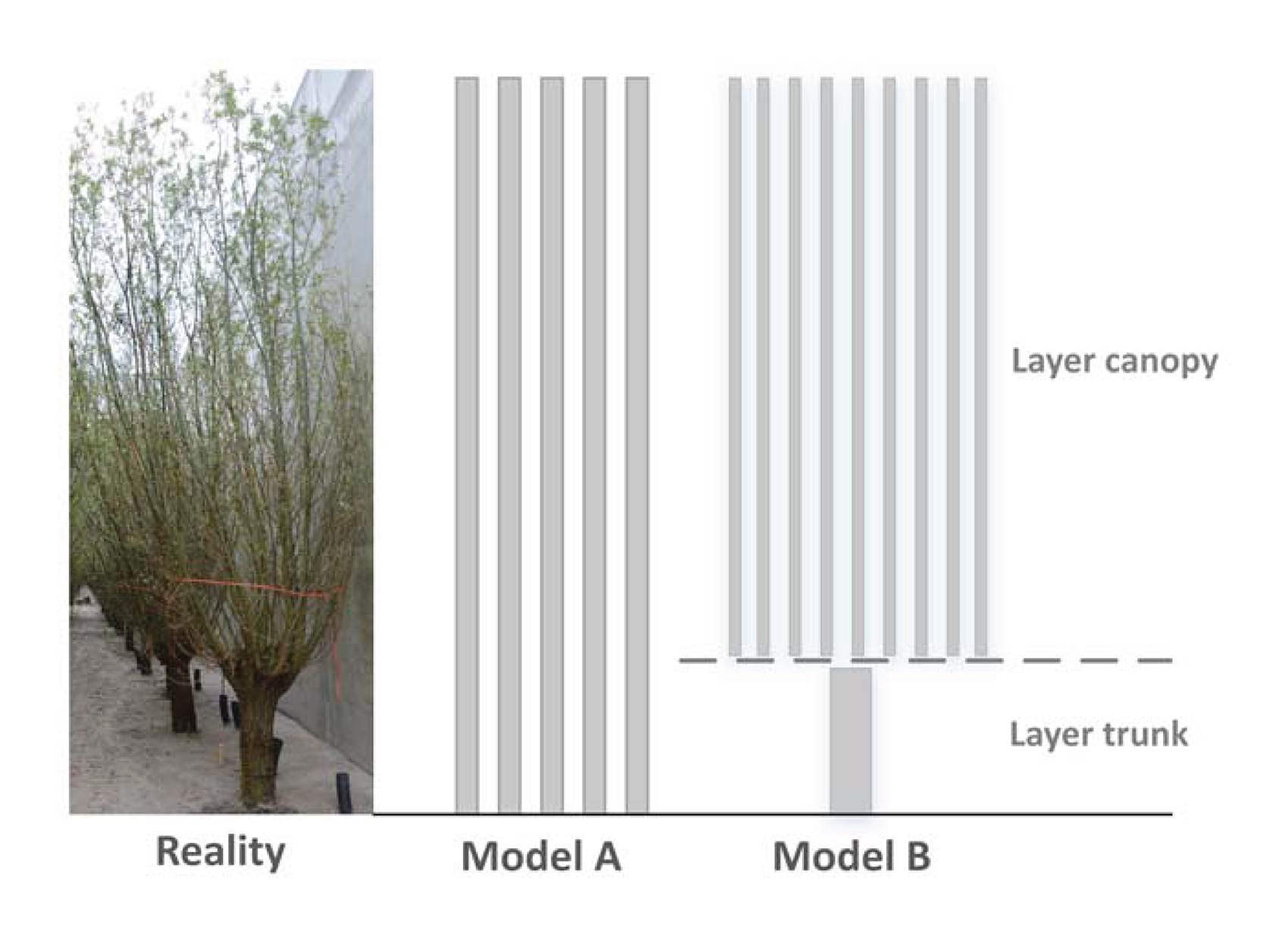
Figure 1. Simple vegetation quantification. Two examples of schematizing a pollard willow tree, namely using a one-layered (Model A) or two-layered model (Model B).

The purpose of this study is to compare different methods for quantifying the frontal-surface area of woody vegetation and present their effect on the wave damping predictions. We use data from large-scale flume experiments with live willow trees under storm conditions, where significant wave heights, H_m0, up to 1.5 m were tested (van Wesenbeeck et al., 2022). Both manual measuring techniques and Terrestrial Laser Scanning (TLS) were conducted during these physical experiments, these are described in Section 3. The frontal-surface area estimation from the TLS data is compared to tree models (i.e., simplified representations of the tree structure). These tree models are developed by combining manual measurements and allometric relations, which are also included in Section 3. Afterwards, we use SWAN to calculate the wave damping corresponding to the different tree models and TLS output. These results are compared to the measured wave damping from the large-scale experiments in Section 4. Finally, methods for quantifying vegetation frontal-surface area, and recommendations for further research are suggested in Section 5.

2. Theoretical Background

2.1. Wave Attenuation by Vegetation

Many studies predicted the wave attenuation by vegetation using an increased bottom friction coefficient (e.g., Hasselmann and Collins, 1968; Quartel et al., 2007), while other studies (e.g., Dalrymple et al., 1984; Kobayashi et al., 1993) represented the vegetation as an array of cylinders, considering the wave forcing on these structures. The latter approach (i.e., cylinder approach) relates the wave attenuation to the plant geometry (i.e., the vegetation height, diameter and density), which is preferred over the former. Studies such as Dalrymple et al. (1984) used the time-averaged energy conservation equation. Here, the wave energy dissipation by vegetation, ϵ_v, is due to the work done by the waves on the vegetation, integrated over the submerged vegetation height. The time-averaged rate of wave energy dissipation per unit horizontal area becomes:

$\begin{array}{ll}\frac{\partial }{\partial x}\left(\frac{1}{8}\rho g{H}^2{c}_g\right)={ϵ}_v,& (1)\end{array}$

$\begin{array}{ll}{ϵ}_v=\overline{{\displaystyle {\int }_{-h}^{-h+h_v}}Fudz},& (2)\end{array}$

The resulting force on the vegetation is given by the Morison equation (Morison et al., 1950):

$\begin{array}{ll}{F}_x=F_D+F_i=\frac{1}{2}\rho C_D{b}_{v}Nu\left|u\right|+\frac{\pi }{4}\rho C_M{b}_v^{2}N\frac{\partial u}{\partial t},& (3)\end{array}$

where F_D is the drag force and F_i is the inertia force. The Morison equation is solely suitable for determining the drag forces on slender objects (neglecting diffraction of waves around the object). We can still use this equation for predicting drag forces on trees with low canopy densities (i.e., no porosity effects namely effects of blockage and sheltering) (Etminan et al., 2019), and the ratio between the wave length and the diameter of the individual branches is small. Furthermore, most of the studies assume linear wave theory to be valid within vegetation fields; therefore, the total force on the vegetation is solely due to the drag forces as the inertia forces are out of phase with the velocity signal. Dalrymple et al. (1984) found an analytical solution for the wave height evolution through a vegetation field. His study focused on vegetation on a flat bottom subject to regular waves. This application has been extended by Mendez and Losada (2004), accounting for sloping bottom and irregular waves. The wave height decay through a vegetation field can be determined with the following equation (Mendez and Losada, 2004):

$\begin{array}{ll}\frac{H_{rms}}{H_{rms,in}}=\frac{1}{1+\beta X},& (4)\end{array}$

with the wave attenuation coefficient, β, as

$\begin{array}{ll}\beta =\frac{1}{3\sqrt{\pi }}\widetilde{C_D}{b}_{v}Nk\frac{{sinh}^{3}k{h}_v+3sinhk{h}_v}{(sinh2kh+2kh)sinhkh}{H}_{rms,in},& (5)\end{array}$

where H_rms is the root-mean-square wave height behind the vegetation field, H_{rms, in} is the incoming root-mean-square wave height (in front of the forest), X is the distance inside the forest, $\widetilde{C_D}$ is the bulk drag coefficient, N is the number of vegetation stems per horizontal area, b_v is the average diameter of the individual stems, k is the wave number, h_v is the height of the vegetation that is submerged, and h is the water depth. To date, the formulation of Mendez and Losada (2004) is widely applied and one can vary the vegetation parameters in space in the spectral version of this vegetation dissipation model.

Suzuki (2011) adapted Equation (5) such that the vertical structure of the vegetation can be taken into account (i.e., C_D, b_v and N can vary over intervals along the vertical). This is implemented in numerical wave models such as SWAN (phase-averaged model) (Suzuki, 2011). For other wave models, such as SWASH (phase-resolving model), the wave dissipation due to vegetation is based on the Morison equation as function of time, and requires also the same geometric information of the trees as vegetation input (i.e., N and b_v).

The bulk drag coefficient is an important, but an uncertain parameter (Kobayashi et al., 1993), as it generally accounts for the neglected processes. For example, we usually assume rigid cylinders, thus neglecting vegetation motion, which influences the relative velocity. Obviously, this becomes less valid for relatively flexible vegetation and can influence the wave attenuation by these fields. Furthermore, simplifications of vegetation geometry can also affect the wave attenuation processes. Nevertheless, several studies reveal relations between the bulk drag coefficient and dimensionless hydraulic parameters, such as the Reynolds number, Re (e.g., Hu et al., 2014) and the Keulegan-Carpenter number, KC, (e.g., Jadhav et al., 2013). Both Re and KC are predictors for the wake structures behind the vegetation (Sumer and Fredsoe, 1998). KC is also a measure for the relative importance between drag and inertia. These studies generally show that C_D decreases with increasing KC and Re. In addition, other studies find better relations with non-dimensional parameters containing also vegetation characteristics such as the vegetation submergence ratio (Mendez and Losada, 2004) and the spacing between cylinders (Suzuki, 2011). These relations make it possible to chose a value for the bulk drag coefficient accordingly. In the case of woody vegetation with enough spacing between branches without motion, one can expect the C_D values to be similar to that of rigid vertical cylinders, which holds a nearly constant value of ≈ 1.0 to 1.2 in the sub-critical flow regime (10³ ≤ Re ≤ 10⁵) (Sumer and Fredsoe, 1998; van Wesenbeeck et al., 2022).

2.2. Quantifying Vegetation

Knowing the vegetation densities (N) and average diameters (b_v) in space is usually sufficient vegetation input for wave damping models for large enough Reynolds numbers, keeping in mind that the bulk drag coefficient can be used for calibration. An example of two rather simple representations of a pollard willow tree is shown in Figure 1. Unlike the simplified description in these wave damping models, the realistic branch structure of woody vegetation is difficult to capture by means of a single diameter and density. It is difficult to get accurate approximations of these values, especially for woody vegetation because these strongly vary in space. Furthermore, the individual branches are also characterized by an angle (i.e., direction in which they grow) with respect to the incoming waves, which also complicates determining the 'projected' surface area. Alternatively, the frontal-surface area distribution of all the branches, A_v(z) = b_v.N, gives a better approximation of the entire tree structure. Hence, this research focuses on determining this parameter (van Wesenbeeck et al., 2022).

Obtaining vegetation parameters can be done in different ways, namely: by conducting manual measurements or using remote sensing techniques (e.g., optical techniques and lidar, which can be spaceborn, aerborne, or terrestrial); each having its own advantages and disadvantages.

Manual measurements can be categorized into destructive (i.e., for biomass measurements) and non-destructive measures (Nordh and Verwijst, 2004). The latter is a simple way of obtaining geometric information of trees and, accordingly, for calculating wave attenuation. For example, the density and diameters in a certain volume can be determined, after which a vertical and horizontal average value may be used. This is generally seen as a valid way to quantify vegetation and has been used in several studies (e.g., Jadhav et al., 2013; Möller et al., 2014; Ozeren et al., 2014). Some studies indicate that the vertical variation of vegetation parameters is important to consider (Ozeren et al., 2014), and this vertical variation is already incorporated into numerical models (Suzuki, 2011). Thus, a certain spatial resolution is needed depending on the vegetation type, and conducting hand measurements often becomes tedious.

Although solely hand measurements can be inefficient, we can still indirectly extent this data by using it as input for tree allometric relations. These are mainly formulations to obtain difficult tree parameters, such as tree height, through an relatively easy measured parameter such as the diameter at breast height. It is shown to work well for characterizing mangrove roots (Ohira et al., 2013). A branching method, which also uses tree allometry, is developed by Järvelä (2004) to calculate the area of trees. This method stems from the Strahlers ordering scheme, originally applied on river systems and later on tree structures (McMahon and Kronauer, 1976). This scheme starts at the smallest order ('finger-tip'), where two small bifurcations of the same order meet, they sum up to a higher order stream and so on, until it reaches the highest order stream (Order=n). Certain factors in between orders, also referred to as branching factors, are obtained and used to calculate the total area of a tree. These branching factors are mostly dependent on the tree species. For a detailed description on this branching method, we refer to Järvelä (2004).

Lastly, remote sensing techniques can be used to obtain vegetation parameters. Space-borne and airborne methods are effective for very large-scale measurements, for example identifying the state of the vegetation, but are less accurate for capturing vegetation parameters such as height and canopy structures (Srinivasan et al., 2014). On a smaller scale, optical techniques are commonly used, and provide detailed information on the geometry (e.g., Norris et al., 2017; Maza et al., 2019). This method becomes more difficult and less accurate when dealing with larger objects, such as trees. For tree and forest scale applications, Terrestrial laser scanning (TLS) shows to be a good alternative. A comparison between TLS results and the branching method of Jarvela showed a good agreement in terms of total area of trees, which was afterwards used for determining the flow resistance during floods (Antonarakis et al., 2009).

3. Methods

Section 3.1 describes the large-scale physical experiments, which includes the set-up and measurements of the forest, and of the waves. Different methods for measuring and modeling the frontal-surface area in space result in different estimates for frontal-surface area distributions over height, Av(z). These methods are described in Section 3.2. Results of Av(z), which can follow from combinations of measurements and tree allometry relations, are called tree models in this work. These tree models are used to determine the required input for the wave attenuation model, A_v. Detailed data of the tree parameters and of the wave damping by these trees is used from large-scale physical experiments; hence, direct comparisons could be made between the measured wave attenuation and the calculated wave attenuation.

3.1. Physical Experiments

Full-scale experiments were conducted on live pollard willow trees under storm conditions. These experiments were carried out in a 300-m-long, 5-m-wide and 9.5-m-deep wave flume, where significant wave heights (H_m0) up to 1.5 m were tested. A 40-m-wide forest was created with 32 pollard willow trees (Salix Alba) in front of a concrete levee. These trees formed 16 rows of 2, and were situated on a 85-m-long and 2.33-m-high platform. The platform represented a shallow foreshore, which permitted large wave height-water depth ratios to avoid having wave breaking inside the forest. A more detailed description of the experimental set-up is given in the paper of van Wesenbeeck et al. (2022).

3.1.1. Experimental Setup: Forest

3.1.1.1. Manual Measurements

The pollard willow trees (Salix Alba) were 15 years old with 3-year-old primary branches (i.e., branches that directly sprout from the knot of the tree). These primary branches were categorized into 3 classes (see Figure 2) based on the diameter at their base, D_B (i.e., diameter at the location above the knot), namely: class 1 (D_B > 50 mm), class 2 (20 < D_B ≤ 50 mm) and class 3 (D_B ≤ 20 mm).

FIGURE 2

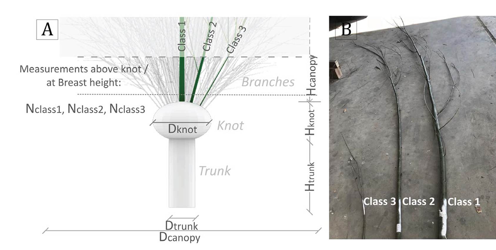
Figure 2. (A) General tree characteristics of the pollard willow, (B) examples of the 3 different diameter classes of branches.

The main tree characteristics were manually measured prior to conducting test series 1 (full canopy with leaves). These include the following measurements:

• General tree characteristics:

• Diameter and height of the trunk (D_trunk, H_trunk)

• Diameter and height of the knot (D_knot, H_knot)

• The number of branches per diameter class (N_class1, N_class2, N_class3)

• Diameter and height of the canopy (D_canopy, H_canopy)

After the experiments, we took the following additional measurements:

• Characteristics of the primary branches:

• The D_B with corresponding total branch length was measured in order to create an allometric relation. Allometric relations are commonly used to estimate tree parameters, which are challenging to measure (such as the branch length), from an easier measurable parameter (such as the diameter at breast height). A random sample size of 340 primary branches out of the entire forest, which in total consists of 2,852 primary branches, was used.

• Diameter decay relations were made for each branch class, as branches have a tapering form. This was achieved by measuring the diameter at increments of 1 meter along the main branch. A random sample size of 30 branches was used (10 branches per branch class).

• Sketches of 9 branches were made. These sketches include the number, length and diameter of all the side branches; and they include the diameter of the main branch at vertical increments of 1 meter.

• Additionally, strength and elasticity measurements were conducted on the primary branches; however, these are not analyzed in the present work.

• Distribution of branch diameter and density over the vertical, by measuring an individual tree (i.e., This tree was from the same location as the tested trees, and contained shoots of the same age), named “Tree S”:

• The general tree characteristics were measured (H_trunk, D_trunk, H_knot, D_knot, N_class1, N_class2, N_class3, D_canopy, H_canopy)

• The number of branches and their diameters were measured at 1 meter vertical increments. This was eventually used to compute the branch density (N) and the average diameter (b_v) within each vertical interval.

3.1.1.2. Terrestrial Laser Scanning

Besides taking manual measurements, we also used Terrestrial laser scanning (TLS). We scanned the forest prior and after each test series to monitor the state of the forest and to detect possible loss of tree biomass. These scans were taken with a FARO FOCUS 3D S 120 scanner from three fixed positions above the flume (Figure 5).

3.1.2. Experimental Setup: Wave Measurements

The tests (T001-T042) were carried out with different wave parameters and vegetation configurations. In total 5 test series (TS) were conducted, namely: TS 1 on the trunks of the trees for low hydrodynamic conditions (i.e., low water levels and wave heights), TS 2 on full canopies with leaves, TS 3 on full canopies without leaves, TS 4 on reduced canopy density without leaves, and TS 5 without willows (calibration tests). A more detailed description of the wave conditions is given in the Supplementary Table S1.

The wave heights in front and behind the forest were measured with two types of wave gauges (i.e., radar wave gauge and resistance wave gauge). The wave damping due to the vegetation is expressed as the ratio between the incoming wave height and the wave height reduction (i.e., the difference in wave height between the tests with vegetation and the tests without vegetation), as applied in van Wesenbeeck et al. (2022):

$\begin{array}{ll}Dr=\frac{(H_{m0,noveg}-H_{m0,veg})}{H_{m0,in}},& (6)\end{array}$

where Dr is the wave damping ratio by vegetation, H_{m0, veg} and H_{m0, noveg} are the measured wave heights with and without vegetation at the location behind the forest, and H_{m0, in} is the measured incoming wave height in front of the forest.

3.2. Methods for Quantifying A_v

3.2.1. Tree Model 1 - Primary Branch Model

The first method considers the primary branches (i.e., main shoots) and their tapering form. Information of the branching structure and side branches is not included, therewith the contribution of the side branches (secondary and tertiary) to the total A_v is neglected. Allometric relations between D_B and the total length of the branches (Section 3.1.1), the total number of branches counted per tree, together with diameter decay relations of the primary branches were used to predict diameter and the total number of branches at vertical increments of 1 m. With this, the frontal-surface area is obtained at vertical increments of one meter for each tree. Hereby it is assumed that the primary branches are oriented perpendicular to the knot, with the largest branches located in the center of the knot (see Supplementary Figure S1).

3.2.2. Tree Model 2 - Branching Model (By Example)

As in tree model 1 the side branches were neglected, a branching method similar to the one by Järvelä (2004) is used to account for the side branches. We made some adjustments based on the measured properties of pollard willows. This method will be illustrated with an example on one tree, named “tree S.”

Firstly, the regular pollarding practice on these trees impacts the tree structure, namely with relatively thick knot and trunk with respect to its branches, deviating from the “natural” willow structure. Therefore, the branches are regarded separately from the trunk, applying the method on the primary branches (excluding the trunk). We first identified the initial parameters for each tree. These are given in Table 1 for tree S. Besides these parameters, we also defined the minimum diameter, d_min of 0.003 m and the height of the canopy, H_canopy of 3.4 m.

TABLE 1

Table 1. Initial parameters of the branches of tree S for the tree simulation.

Secondly, we used the detailed sketches of the branches to obtain three branching factors. These branching factors show the number of side branches that a mother branch can support (R_B), the diameter ratio (R_D) and length ratios (R_L) between subsequent branch orders. These factors are defined as follows: R_B = $\frac{N_{b(m)}}{N_{b(m+i)}}$, R_D = $\frac{D_{(m+1)}}{D_m}$, and R_L = $\frac{L_{(m+1)}}{L_m}$; where m is the child branch, (m+1) is the mother branch, N_b is the number of side branches, D is the diameter, and L is the length of the branch. The obtained branching factors differ per order (Table 2), thus we maintained distinct values per order instead of working with the average values and are assumed constant for all trees.

TABLE 2

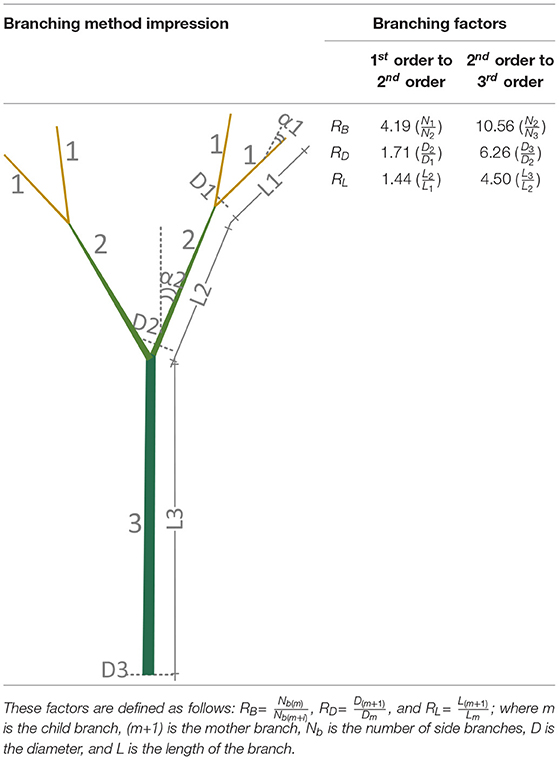
Table 2. Impression of branching method and the resulting branching factors.

Thirdly, the frontal-surface area was determined by applying the branching factors from Table 2 on the initial parameters from Table 1. The highest order branch is generally assigned to the trunk; however, in this work the primary branches are the highest order (3^rd order) as mentioned before. The steps to obtain the total frontal-area can be seen in Table 3. For example, the diameter factor, R_D, is applied on the highest order branch (i.e., the base diameter), D₃, until a diameter of the smallest order branch (d₁) is equal to the minimal diameter (d_min) of ≈ 0.003 m.

TABLE 3

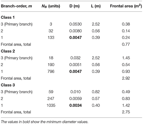
Table 3. Frontal area calculation for all the branches of class 1 (D_B ≤ 50 mm), class 2 ( 20 mm < D_B <50 mm), class 3 (D_B ≤ 20 mm) of tree S.

Fourthly, we applied a factor of 0.5 on the obtained frontal areas of Table 3 to account for the tapering form of the branches, as this is not accounted for in the initial method. Finally, we validated the branching method by applying it to the nine detailed sketches and on the measurements of the individual tree.

The method by Järvelä (2004) solely computes the total surface area of the tree; moreover, it lacks information of the vertical distribution (Järvelä, 2004; Antonarakis et al., 2009). The distribution cannot be determined from these methods as no angles between the branches, no tapering of the diameters, and no positions are considered. To determine the height variation of the surface area, we simulated the random structure of individual branches based on the allometric relations described above. The simulations allow for variations in the branch positions, while still following the branching rules. This results in slightly different branches from each simulation, mimicking “real” trees. The tapering form of the branches is included in the simulation by assuming linear diameter decay along its length.

This tree model was validated as some tree parameters such as the angles of the side branches, the start positions of the primary branches on the knot, and the start positions of the side branches on their mother branch, do not have constant values and their distributions are not known. Thus, we validated this tree model against the hand measurements done on a single pollard willow (Tree S), keeping in mind that from these hand measurements we could also obtain ∑b_{v, i} at vertical increments of 1 m. The same step-size (1 m) was used to calculate ∑b_{v, i} from the structure as simulated with tree model 2. Furthermore, only diameters larger than 4 mm were considered, as this was the cut-off diameter applied in the hand measurements.

As mentioned above, the angles between branches were not measured. Still, this may influence the value of A_v(z). Hence, a range of angles between the side branches were simulated from 10° to 45° with 5° increments to determine the influence of the angles, and to chose a suitable value. The outcome is given in Figure 3. The angle between 1st and 2nd order branches, α₁ = 30°, and the angles between 2nd and 3rd order branches, α₂ = 25°.

FIGURE 3

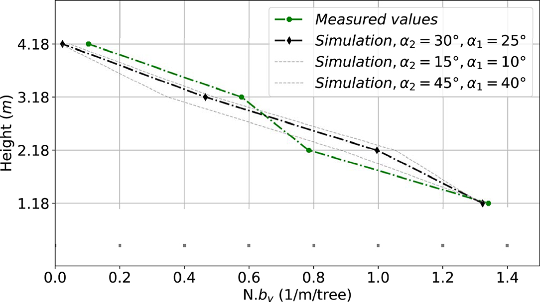
Figure 3. Validation of tree simulations.

Finally, the frontal-surface area variation along the height, A_v(z), was calculated. This is defined as the projected surface area of the simulated branches perpendicular to the incoming waves (see Figure 4). Thus, these three-dimensional simulations take the branch angles, positions and diameter decay into account.

$\begin{array}{ll}\Delta A_v=\frac{1}{2}*\Delta s^{\prime }*(D_{s,i}+D_{s,i+1}),& (7)\end{array}$

$\begin{array}{r}\alpha =\text{arccos}\frac{dZ}{\sqrt{d{X}^2+d{Y}^2+d{Z}^2}}\\ \omega =\text{arctan}\frac{dX}{dZ}\\ \Delta s=\frac{\Delta z}{cos\alpha }\\ \Delta s^{\prime }=\frac{\Delta z}{cos\omega }\end{array}$

FIGURE 4

Figure 4. Schematic of the coordinate system used for calculating A_v with the incoming waves from the positive y-direction. P is the endpoint of the branch, and P' is the projected branch perpendicular to the incoming waves.

3.2.3. Terrestrial Laser Scanning - Post Processing

Data from the scans of the leaf-less condition of the trees were used to obtain A_v(z). This vegetation state coincides with the characteristics that we observe during extreme conditions, which are high hydraulic loads and leaf-less trees (winter season). Not to mention, scans during leaf-on conditions are less suitable to map the vegetation as most of the laser beams are directly blocked in the outer layers of the tree by the leaf density (see Figure 6) and leaves do not add significantly to the wave damping (van Wesenbeeck et al., 2022). Figure 5 shows the entire forest without leaves and the 3 positions in the flume from which the TLS scans were created.

FIGURE 5

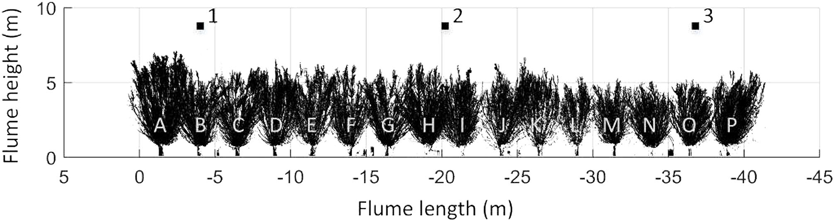
Figure 5. Side view of the 3D-point cloud of the entire forest without leaves. The tree names (A-P) and the laser scanner positions (1-3) are illustrated.

FIGURE 6

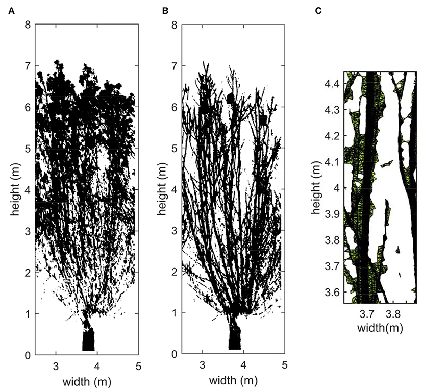
Figure 6. (A) Tree A1 with leaves, (B) tree A1 without leaves, (C) surface area by alpha shape function (α = 0.01).

The post-processing of the point cloud data included sub-sampling, segmentation and filtering of the point cloud, performed in CloudCompare. Segmentation was done to remove excess information (e.g., measuring equipment, and flume walls) and sub-sampling was needed for the sake of work-ability of the point cloud. Afterwards, the point cloud data of each tree was analyzed separately and the frontal area (i.e., does not include for the angles of the branches relative to the incoming waves) was constructed using alpha−shape function, which is a built-in function in MATLAB. This function uses an alpha parameter to control how it creates the bounding region around the 3D-point cloud. An alpha shape value of 0.01 is used in this study, shown in Figure 6.

3.3. Simulating Wave Attenuation and Bulk Drag Coefficients

The Morison equation is solely suitable for determining the drag forces on slender objects (neglecting diffraction of waves around the object), but can be used for predicting drag forces on trees as well. In this study, the forest is characterized by low canopy densities of around 13 branches per m². The average spacing, ΔS becomes 28d, with d = 10mm as the average branch diameter. The density parameter as described in Nepf (1999), ad = d²/ΔS², is approximately 0.001, indicating a relatively sparse forest; hence, we can assume no porosity effects (i.e., blockage and sheltering). Thus, the drag coefficient can be considered similar to that of a single cylinder (Etminan et al., 2019). In addition, the ratio between the wave length and the diameter is small, following the characteristic of slender objects.

SWAN in 1D-mode is used in this study to simulate the waves through the forest. The SWAN model was defined in Cartesian coordinates with a spatial discretization of 1 meter. The model is forced with identical JONSWAP spectra to those measured at the deep water locations in the experiments (WHM01-03). SWAN was executed without accounting for wind growth, white capping, refraction, diffraction, quadruplets, triads and turbulence dissipation, as these processes are not relevant in this flume experiment. On the other hand, frequency shifting in frequency space, bottom friction with a roughness constant of 0.07 m²s⁻³, wave breaking, and vegetation dissipation were activated. The wave energy dissipation through vegetation fields accounts for the vertical structure of the vegetation and follows the action balance formulation, as shown in Suzuki (2011). Following the same manner, the energy dissipation by vegetation becomes:

$\begin{array}{l}\langle {ϵ}_v\rangle ={\displaystyle \sum _{i=1:I}}\frac{1}{2\sqrt{\pi }}\rho {\tilde{C}}_D(\frac{gk}{2\sigma }{)}^3\\ A_{veg,i}\frac{({sinh}^{3}k{\alpha }_{i}h-{sinh}^{3}k{\alpha }_{i-1}h)+3(sinhk{\alpha }_{i}h-sinhk{\alpha }_{i-1}h)}{3kcosh{kh}^3}{H_s}^3,& (8)\end{array}$

where 〈ϵ_v〉 is the averaged wave energy dissipation due to vegetation; $\widetilde{C_D}$ the bulk drag coefficient, g the gravitational acceleration constant; k the mean wave number; α_i the ratio between the depth at the top of the vertical layer i and the total water depth (α_i ≤ 1), where i = 1 represents the lowest vertical layer and i = I the highest vertical layer; h the water depth; H_{s, in} the significant wave height; and A_{veg, i} the total frontal width of vegetation perpendicular to the waves for layer i per unit area. Varying this vegetation parameter A_{v, i}, according to the different tree models, will result in different wave attenuation outcome.

The bulk drag coefficient, $\widetilde{C_D}$, is important for predictive wave models and is therefore often estimated in studies on vegetation (e.g., Suzuki, 2011; Maza et al., 2015). In this work, the SWAN model is tuned with the measurements such that the modeled wave damping corresponds to the measured wave damping behind the forest. To achieve this, the tuning parameter, namely the bulk drag coefficient, is calibrated using exhaustive search. We made a distinction between the drag coefficient of the canopy (C_{D, can}) and the trunk (C_{D, tr}) for the tests with high water levels. For these high water level tests, the drag coefficient of the trunk is set to a constant value of 1.2 (Wieselsberger, 1921). The SWAN set-up is made following the same approach as described in van Wesenbeeck et al. (2022). This is repeated for different vegetation input [i.e., A_v(z)] from the tree models and TLS results.

4. Results

This section shows general characteristics of the 32 pollard willow trees (Section 4.1), and the characteristics of the resulting tree models (Section 4.2). We analyzed the frontal-surface area, A_v(z) of each tree model, and afterwards we calculated the corresponding wave attenuation and compared these results. In addition, the relation between Keulegan- Carpenter number (KC) and drag coefficient (CD) for each tree model is presented (Section 4.5). This provides us more insight into the errors of different tree models and their effects on predicting wave attenuation.

4.1. General Characteristics of Pollard Willows

From the manual measurements it follows that the smaller primary branches (Class 3) take up a large portion of the total number of branches in a pollard willow tree (64 %), while the larger primary branches (Class 1) only account for 3 % of the total number of shoots. Therefore, a larger data set could be obtained for the smaller branches. The fraction of each diameter class is given in Figure 7A with corresponding 95%-confidence interval. Furthermore, the gathered data of the D_B is plotted in Figure 7B, which includes for the average value and the 95%- confidence interval.

FIGURE 7

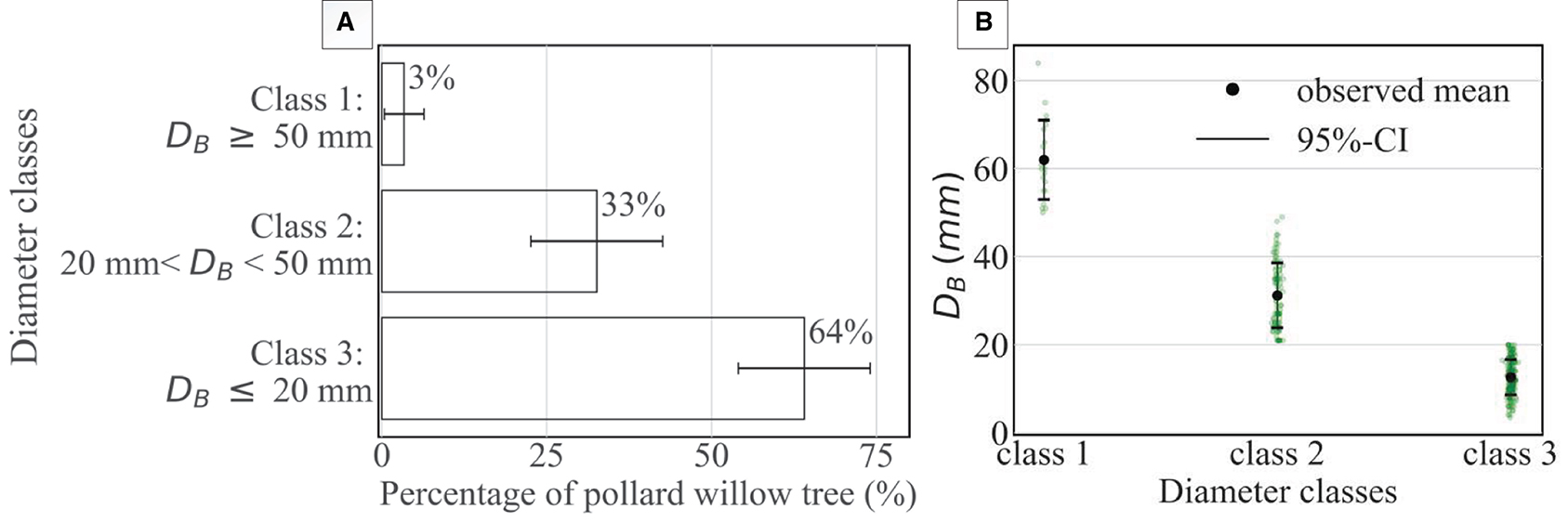
Figure 7. (A) Distribution of diameter classes for a pollard willow tree, (B) diameter range found for each class.

Other tree parameter such as the D_b, N_high and L_high, are given in Supplementary Table S2.

4.2. Tree Model Results

4.2.1. Tree Model 1: Primary Branches

Solely considering the primary branches of the pollard willow trees is a relatively simple way of mapping the vegetation. Besides this, relatively less wave attenuation is expected from the smaller side-branches as these are more flexible than the primary branches. The manual measurements done at breast height (i.e., the number of branches per class), the allometric relation between D_B and branch length, and the diameter-decay relations were the main input for this tree model. We assumed an average diameter at breast height for each class (see Figure 7B). The D_B-length relation, diameter-decay relation, and a simplification of the tree without side-branches (tree model 1), are shown in Figure 8. This model is considered as the lower limit of the frontal-surface area as it only accounts for the main branches (neglecting the side branches). It was initially expected to give a reasonable estimate of the total A_v; on the contrary, the comparison to the other tree model that follows hereafter shows that this is not the case.

FIGURE 8

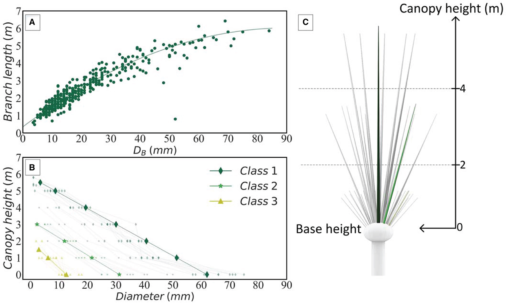
Figure 8. (A) The relation between the diameter at the base of the knot (D_B) and the branch length for 340 branches (containing all classes), (B) the diameter decay along the length of the branch for 10 branches of each class (class 1, 2, and 3), (C) impression of tree model 1 (i.e., only accounting for main branches).

4.2.2. Tree Model 2: Branching Method

The branching method uses RNG to describe the branch structure for all branches larger than ≈ 3 mm, which is used to create tree model 2. To statistically estimate the A_v(z), trees were simulated in Python to generate random branches that follow the branching rules shown in Table 2. The parameters from Supplementary Table S2 are input for generating the branches. An example of a generated branch from each class is shown in Figure 9A. Figure 9B illustrates tree model 2, which is formed by these generated branches positioned on the knot. In Figure 11A the A_v(z) as sampled from the generated trees is shown. As each realization yields a different A_v(z), the output is a distribution for which the mean and the 95% confidence interval are determined.

FIGURE 9

Figure 9. (A) An example of 3 simulated branch classes, (B) impression of one simulated tree which consists of a trunk, a knot and multiple branches of each class.

4.3. TLS Correction Factor

The comparison of A_v (Figure 11B) showed an overall underestimation by the TLS results. Though, the TLS showed an overestimation in the upper layers of the trees. This suggests that occlusion due to the canopy density is the main reason for the observed errors in the lower canopy layers. A correction factor was applied on one tree at the edge of the forest to improve the TLS results by accounting for the percentage of blocked laser beams.

$\begin{array}{ll}{A}_{TLS,new,n}=A_{TLS,n}*f_{cor,n},& (9)\end{array}$

$\begin{array}{ll}{f}_{cor,n}=\frac{N_t}{N_t-{\displaystyle {\sum }_{i=n+1}^{i=m}}N},& (10)\end{array}$

where A_{TLS, n} is the area obtained from the 3D-point cloud in layer n, f_cor is a correction factor based on the number of blocked laser beams, N_t is the total amount of laser points send out by the laser scanner, and N is the number of laser points blocked in the layer before reaching layer n. The correction increased the A_{v, tot} with 2.45 m². However, this correction could only be applied to trees near the laser scanner positions as occlusion by neighboring trees could be neglected. We applied this to tree P1 as this tree is also most likely not hit by laser beams other than the laser scanner nearest to it (see Figure 10).

FIGURE 10

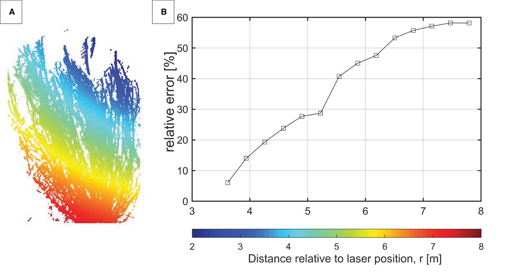
Figure 10. (A) Tree P1 with, (B) corresponding graph containing the relative error of the laser scanner as function of the penetration distance of the beam, r. The colors and the horizontal axis indicate the distance from the laser scanner.

4.4. Comparing Frontal-Surface Area

The three different tree models are first compared considering their frontal-surface area distributions, shown in Figure 11B. All the tree models are set to a similar resolution (i.e., namely at vertical increments of 1 m) of the results to get a more clear comparison between the models. It shows that side branches amount to at least ≈ 25 % more A_{v, tot} than only the primary branches. Furthermore, the TLS results underestimate the canopies total frontal-surface area compared to the other tree models. The underestimation by the TLS is mainly seen in the lower layers of the trees, while in the upper layers there is an overestimation.

FIGURE 11

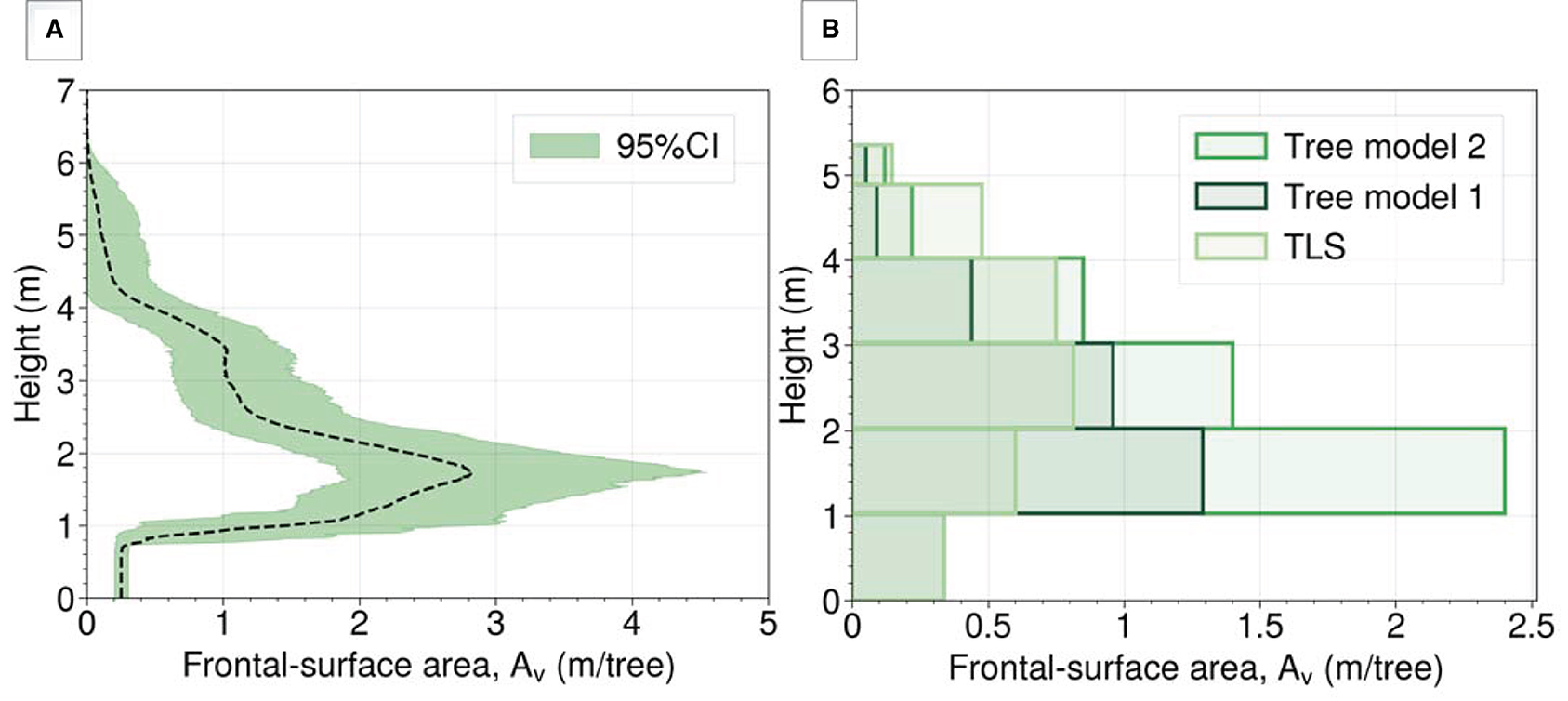
Figure 11. (A) The average frontal-surface area (A_v) of the 32 trees in the large-scale experiments with 95% confidence interval using tree model 2, (B) frontal-surface area comparison of the tree models, considering the average tree without leaves in the wave flume.

4.5. Comparing Wave Attenuation

A strong relation is found between $\widetilde{C_D}$ and the Keulegan- Carpenter number (KC). The KC number is usually calculated as follows: $KC=\frac{U\times T}{L}$, where U is the orbital velocity, T is the wave period and L is the average diameter of the object. For determining KC, we chose the maximum horizontal orbital velocity based on linear waves U_0max, and T_m02 as a representative wave period of the wave spectrum. The definition of KC is non-trivial for realistic tree structures, as these structures are characterized by a distribution of branch diameters that varies over the height. The KC number in this work is calculated at vertical increments of 1 m and averaged over the height.

The results show a decrease of $\widetilde{C_D}$ with increasing KC numbers (Figure 12). Furthermore, the differences in $\widetilde{C_D}$ between the tree models are a consequence of different frontal-surface area distributions. Tree model 1, which is considered as the lower limit for the frontal-surface area, shows larger $\widetilde{C_D}$ values relative to tree model 2, due to its lesser frontal-surface area. The largest $\widetilde{C_D}$ values are observed for tree model 3. This is according to expectation, since the TLS method underpredicts the frontal-surface area of the trees (Section 4.4).

FIGURE 12

Figure 12. Relation between C_D and KC for tree model 1 (only the Primary branches), tree model 2 (primary branches including the side branches), and tree model 3 (TLS measurements).

5. Discussion and Conclusion

Globally, considerable claims are made of how trees, such as mangroves and fresh water trees, reduce impact of waves during extreme storms and tsunamis (EJF, 2006). Most research on wave attenuation by vegetation focused on investigating hydrodynamics around the vegetation structure, whereas less attention is given to vegetation parameters and methods to quantify these structures (e.g., Huang et al., 2011; Wu and Cox, 2015). Vegetation, such as in salt marshes, is generally quantified in a simplified manner using a spatial average diameter (b_v) and density (N). For example, studies on mangrove forests used similar approaches, where single values for the density and diameter were used to represent the entire structure (e.g., Phan et al., 2019) or used single values per layer to represent the roots, trunk and canopy separately (e.g., Vo-Luong and Massel, 2008; Narayan et al., 2011; Ismail et al., 2012). More thorough quantification of especially complex canopies seems to be lacking, but is needed to obtain insight in processes that determine wave attenuation during extremes accurately. For woody vegetation (e.g., willows and mangroves) the frontal-surface area parameter, A_v(z) is an useful way of quantifying this. Some studies have described vegetation using similar parameters concerning the tree frontal area (e.g., Maza et al., 2017, 2019). However, these solely considered damping through roots and trunks, neglecting the canopy.

Previously, large-scale experiments were conducted on a well-defined 40-m-long willow forest (Salix Alba) for which the wave attenuation during storm conditions was determined (van Wesenbeeck et al., 2022), showing that most of the wave damping occurred at mid-water levels through the canopies of the trees. This is where most of the biomass and surface-frontal area was present; hence, improving our estimates of the entire vegetation structure and developing methods to quantify this will improve predictability of wave attenuation by vegetation for different water levels and wave heights. We used these large-scale experiments to obtain more insight in methods to extract A_v(z) of the trees, using both manual measurements and terrestrial laser scanning (TLS). Manual measurements executed on all the branches at vertical increments of 1 meter, are relatively simple measurements, but tedious to conduct on every tree. The accuracy of these measurements depends on the size of the vertical increments (i.e., layer thickness). With this, the diameter decay along the vertical is taken into account to a certain extent. However, the angles of the branches are neglected and side branches that are within the layers are also neglected.

Using simple manual measurements as input for allometric relations for trees, is an efficient way of including side branches. Based on this, a three-dimensional tree model is created (included positions and angles of the branches), which was used to determine the frontal-surface area distribution in the vertical, A_v(z). For this method, it is important to point out that the initial tree parameters and branching factors used in this research are applicable for “pollard” willows with 3-year-old shoots (Salix Alba); these values are likely to differ for "natural" willows of the same species. The simulations from this method can nevertheless be used to obtain a more thorough representation of the trees for numerical and physical models.

The side branches are relatively flexible branches, leading to more extreme branch motion. This in turn, can lower the significance that these small branches may have on attenuating waves. On the other hand, it was found that the side branches could take up to 25% of the total frontal-surface area of these trees. Thus, including these branches in tree models may be necessary for wave attenuation predictions.

A more efficient method for assessment of A_v(z) could be through TLS measurements. The TLS is a practical method to conduct measurements on a forest scale and has the potential to be combined with satellite data into useful parameters for wave damping models. However, the results of the TLS depend on the post-processing and in our case, the chosen α- value. We showed that the TLS underestimates the frontal-surface area, especially near the trunk region where branch densities are largest, which is mainly due to shadowing effects. However, this can be corrected by applying a factor that accounts for the shadowing phenomenon (blockage of the laser beams by high branch densities). These findings encourage further research on the TLS as it is a promising measuring technique for mapping large heterogeneous forests in the field. For this, it is recommended to position the TLS in the direction of the incoming waves to investigate the blockage factor in more depth.

Furthermore, a decrease in bulk drag coefficient with increasing Keulegan-Carpenter number (KC) was shown, which is a trend found also in other vegetation studies (e.g., Anderson, 2011; Ozeren et al., 2014; Etminan et al., 2019). The numerical model validation showed large differences in wave attenuation for different tree models and a corresponding large range in bulk drag coefficients, especially for lower KC numbers. This suggests that the discrepancies between the tree models in terms of frontal-surface area is significant for the wave attenuation. A range of C_D between 0.94 and 1.70 for high KC numbers was obtained, emphasizing the importance of reliable frontal-surface area distributions.

Thus, having feasible methods to obtain reliable frontal-surface area of vegetation fields is relevant for reliable wave predictions. This will increase the potential of implementing hybrid flood defenses, existing of coastal or riparian vegetation and engineered structures, such as embankments or levees. Only a combination of more accurate measurements on vegetation, data and modeling can be used to systematically obtain more insight in what vegetation can actually contribute to flood risk reduction during average and more extreme conditions.

Data Availability Statement

The raw data supporting the conclusions of this article will be made available by the authors, without undue reservation.

Author Contributions

BH and BW designed the research project. The calculations and analysis were performed by SK and supervised by BH. JA carried out the swan simulations. SK carried out the tree simulations and wrote the manuscript with input from all authors. All authors discussed the final results, contributed to the manuscript revision, and approved of the submitted version.

Funding

This study was done within the research program WOODY, number 17194, which is financed by the Dutch Research Council (NWO) via the Open Technology Program.

Conflict of Interest

BH, JA, and BW were employed by Deltares.

The remaining author declares that the research was conducted in the absence of any commercial or financial relationships that could be construed as a potential conflict of interest.

Publisher's Note

All claims expressed in this article are solely those of the authors and do not necessarily represent those of their affiliated organizations, or those of the publisher, the editors and the reviewers. Any product that may be evaluated in this article, or claim that may be made by its manufacturer, is not guaranteed or endorsed by the publisher.

Acknowledgments

We thank van Oord, Boskalis, Rijkswaterstaat, World Wildlife Fund, Stowa, and VP Delta for their contributions to this research. We thank Ceylan Cete and Hassan Niazi for helping with the measurements on the trees. The simulations were carried out on the Dutch national e-infrastructure with the support of SURF Cooperative under project EINF-666 Emerging technologies for Nature Based solutions in coastal waters, and we acknowledge support by GNU Parallel (Tange, 2021).

Supplementary Material

The Supplementary Material for this article can be found online at: https://www.frontiersin.org/articles/10.3389/fmars.2022.820846/full#supplementary-material

References

Anderson, M.E, McKee Smith, J, and McKay, S.K. (2011). Wave Dissipation by Vegetation. US Army Corps of Engineers. 8, 14–15. Available online at: https://erdc-library.erdc.dren.mil/jspui/bitstream/11681/1896/1/ERDC-CHL-CHETN-I-82.pdf

PubMed Abstract | Google Scholar

Antonarakis, A. S., Richards, K. S., Brasington, J., and Bithell, M. (2009). Leafless roughness of complex tree morphology using terrestrial lidar. Water Resour. Res. 45, 1–14. doi: 10.1029/2008WR007666

CrossRef Full Text | Google Scholar

Dalrymple, R. A., Kirby, J. T., and Hwang, P. A. (1984). Wave diffraction due to areas of energy dissipation. J. Waterway Port Coastal Ocean Eng. 110, 67–79. doi: 10.1061/(ASCE)0733-950X(1984)110:1(67)

CrossRef Full Text | Google Scholar

EJF (2006). MANGROVES: Nature's Defence Against TSUNAMIS- A Report on the Impact of Mangrove Loss and Shrimp Farm Development on Coastal Defences. London, UK: Environmental Justice Foundation

Google Scholar

Etminan, V., Lowe, R. J., and Ghisalberti, M. (2019). Canopy resistance on oscillatory flows. Coastal Eng. 152, 11–12. doi: 10.1016/j.coastaleng.2019.04.014

CrossRef Full Text | Google Scholar

Hasselmann, K., and Collins, J. (1968). Spectral dissipation of finite-depth gravity waves due to turbulent bottom friction. J. Mar. Res.26, 77–85.

Google Scholar

He, F., Chen, J., and Jiang, C. (2019). Surface wave attenuation by vegetation with the stem, root and canopy. Coastal Eng. 152, 103509. doi: 10.1016/j.coastaleng.2019.103509

CrossRef Full Text | Google Scholar

Hu, Z., Suzuki, T., Zitman, T., Uittewaal, W., and Stive, M. (2014). Laboratory study on wave dissipation by vegetation in combined current-wave flow. Coastal Eng. 88, 131–142. doi: 10.1016/j.coastaleng.2014.02.009

CrossRef Full Text | Google Scholar

Huang, Z., Yao, Y., Sim, S. Y., and Yao, Y. (2011). Interaction of solitary waves with emergent, rigid vegetation. Ocean Eng. 38, 1080–1088. doi: 10.1016/j.oceaneng.2011.03.003

PubMed Abstract | CrossRef Full Text | Google Scholar

Ismail, H., Abd Wahab, A. K., and Alias, N. E. (2012). Determination of mangrove forest performance in reducing tsunami run-up using physical models. Natural Hazards 63, 939–963. doi: 10.1007/s11069-012-0200-y

CrossRef Full Text | Google Scholar

Jadhav, R. S., Chen, Q., and Smith, J. M. (2013). Spectral distribution of wave energy dissipation by salt marsh vegetation. Coastal Eng. 77, 99–107. doi: 10.1016/j.coastaleng.2013.02.013

CrossRef Full Text | Google Scholar

Järvelä, J.. (2004). Determination of flow resistance caused by non-submerged woody vegetation. Int. J. River Basin Manage. 2, 61–70. doi: 10.1080/15715124.2004.9635222

CrossRef Full Text | Google Scholar

Jonkman, S. N., Hillen, M. M., Nicholls, R. J., Kanning, W., and Van Ledden, M. (2013). Costs of adapting coastal defences to sea-level rise - New estimates and their implications. J. Coastal Res. 29, 1212–1226. doi: 10.2112/JCOASTRES-D-12-00230.1

CrossRef Full Text | Google Scholar

Kobayashi, N., Raichle, A., and Asano, T. (1993). Wave attenuation by vegetation. J. Waterway Port Coastal Ocean Eng. 119, 30–48. doi: 10.1061/(ASCE)0733-950X(1993)119:1(30)

CrossRef Full Text | Google Scholar

Maza, M., Adler, K., Ramos, D., Garcia, A. M., and Nepf, H. (2017). Velocity and drag evolution from the leading edge of a model mangrove forest. J. Geophys. Res. Oceans 122, 9144–9159. doi: 10.1002/2017JC012945

CrossRef Full Text | Google Scholar

Maza, M., Lara, J. L., and Losada, I. J. (2019). Experimental analysis of wave attenuation and drag forces in a realistic fringe Rhizophora mangrove forest. Adv. Water Resour. 131, 103376. doi: 10.1016/j.advwatres.2019.07.006

CrossRef Full Text | Google Scholar

Maza, M., Lara, J. L., Losada, I. J., Ondiviela, B., Trinogga, J., and Bouma, T. J. (2015). Large-scale 3-D experiments of wave and current interaction with real vegetation. Part 2: experimental analysis. Coastal Eng. 106, 73–86. doi: 10.1016/j.coastaleng.2015.09.010

CrossRef Full Text | Google Scholar

Mazda, Y., Magi, M., Ikeda, Y., Kurokawa, T., and Asano, T. (2006). Wave reduction in a mangrove forest dominated by Sonneratia sp. Wetlands Ecol. Manage. 14, 365–378. doi: 10.1007/s11273-005-5388-0

CrossRef Full Text | Google Scholar

McMahon, T. A., and Kronauer, R. E. (1976). Tree structures: deducing the principle of mechanical design. J. Theor. Biol. 59, 443–466. doi: 10.1016/0022-5193(76)90182-X

PubMed Abstract | CrossRef Full Text | Google Scholar

Mendez, F. J., and Losada, I. J. (2004). An empirical model to estimate the propagation of random breaking and nonbreaking waves over vegetation fields. Coastal Eng. 51, 103–118. doi: 10.1016/j.coastaleng.2003.11.003

CrossRef Full Text | Google Scholar

Möller, I., Kudella, M., Rupprecht, F., Spencer, T., Paul, M., Van Wesenbeeck, B. K., et al. (2014). Wave attenuation over coastal salt marshes under storm surge conditions. Nat. Geosci. 7, 727–731. doi: 10.1038/ngeo2251

CrossRef Full Text | Google Scholar

Morison, J. R., O'brien, M. P., Johnson, J. W., and Schaaf, S. A. (1950). The Force Exerted By Surface Waves on Piles. Technical report, California.

Google Scholar

Narayan, S., Suzuki, T., Stive, M., Verhagen, H., Ursem, W., and Ranasinghe, R. (2011). On the effectiveness of mangroves in attenuating cyclone – induced waves. Coastal Eng. 53, 1689–1699. doi: 10.9753/icce.v32.waves.50

CrossRef Full Text | Google Scholar

Nepf, H. M.. (1999). Drag, turbulence, and diffusion in flow through emergent vegetation. Water Resour. Res. 35, 479–489. doi: 10.1029/1998WR900069

PubMed Abstract | CrossRef Full Text | Google Scholar

Nordh, N. E., and Verwijst, T. (2004). Above-ground biomass assessments and first cutting cycle production in willow (Salix sp.) coppice - A comparison between destructive and non-destructive methods. Biomass Bioenergy 27, 1–8. doi: 10.1016/j.biombioe.2003.10.007

CrossRef Full Text | Google Scholar

Norris, B. K., Mullarney, J. C., Bryan, K. R., and Henderson, S. M. (2017). The effect of pneumatophore density on turbulence: a field study in a Sonneratia-dominated mangrove forest, Vietnam. Cont. Shelf Res. 147, 114–127. doi: 10.1016/j.csr.2017.06.002

CrossRef Full Text | Google Scholar

Ohira, W., Honda, K., Nagai, M., and Ratanasuwan, A. (2013). Mangrove stilt root morphology modeling for estimating hydraulic drag in tsunami inundation simulation. Trees Struct. Funct. 27, 141–148. doi: 10.1007/s00468-012-0782-8

CrossRef Full Text | Google Scholar

Oppenheimer, M., Glavovic, B., Hinkel, J., van de Wal, R., Magnan, A., Abd-Elgawad, A., et al. (2019). Sea level rise and implications for low-lying islands, coasts and communities IPCC Special Rep. Ocean Cryosphere Chang. Clim. 355, 126–129. doi: 10.1017/9781009157964.012

CrossRef Full Text | Google Scholar

Ozeren, Y., Wren, D. G., and Wu, W. (2014). Experimental investigation of wave attenuation through model and live vegetation. J. Waterway Port Coastal Ocean Eng. 140, 1–12. doi: 10.1061/(ASCE)WW.1943-5460.0000251

CrossRef Full Text | Google Scholar

Phan, K. L., Stive, M. J., Zijlema, M., Truong, H. S., and Aarninkhof, S. G. (2019). The effects of wave non-linearity on wave attenuation by vegetation. Coastal Eng. 147, 63–74. doi: 10.1016/j.coastaleng.2019.01.004

CrossRef Full Text | Google Scholar

Quartel, S., Kroon, A., Augustinus, P. G., Van Santen, P., and Tri, N. H. (2007). Wave attenuation in coastal mangroves in the Red River Delta, Vietnam. J. Asian Earth Sci. 29, 576–584. doi: 10.1016/j.jseaes.2006.05.008

CrossRef Full Text | Google Scholar

Rog, S. M., Clarke, R. H., and Cook, C. N. (2017). More than marine: revealing the critical importance of mangrove ecosystems for terrestrial vertebrates. Diversity Distribut. 23, 221–230. doi: 10.1111/ddi.12514

CrossRef Full Text | Google Scholar

Srinivasan, S., Popescu, S. C., Eriksson, M., Sheridan, R. D., and Ku, N. W. (2014). Multi-temporal terrestrial laser scanning for modeling tree biomass change. For. Ecol. Manage. 318, 304–317. doi: 10.1016/j.foreco.2014.01.038

CrossRef Full Text | Google Scholar

Sumer, B., and Fredsoe, J. (1998). Hydrodynamics around Cylindrical Structures in Advanced Series on Ocean Engineering, Vol. 33 (Singapore).

Google Scholar

Suzuki, T.. (2011). Wave Dissipation Over Vegetation Fields. Technical report.

Tange, O.. (2021). GNU parallel 20211022 ('sinclair'). Zenodo. doi: 10.5281/zenodo.5593566

CrossRef Full Text | Google Scholar

van Wesenbeeck, B. K., Griffin, J. N., van Koningsveld, M., Gedan, K. B., McCoy, M. W., and Silliman, B. R. (2013). Nature-Based Coastal Defenses: Can Biodiversity Help?, Vol. 5. (Waltham, MA: Elsivier).

Google Scholar

van Wesenbeeck, B. K., Wolters, G., Antolínez, J. A. A., Kalloe, S., Hofland, B., De Boer, W., et al. (2022). Wave attenuation through forests under extreme conditions. Sci. Rep. 12, 1–8. doi: 10.1038/s41598-022-05753-3

PubMed Abstract | CrossRef Full Text | Google Scholar

Vo-Luong, P., and Massel, S. (2008). Energy dissipation in non-uniform mangrove forests of arbitrary depth. J. Mar. Syst. 74, 603–622. doi: 10.1016/j.jmarsys.2008.05.004

CrossRef Full Text | Google Scholar

Vuik, V.. (2019). Building Safety with nature salt marshes for flood risk reduction, in TU Delft University (Delft: Delft University of Technology), 1–5. doi: 10.4233/uuid:9339474c-3c48-437f-8aa5-4b908368c17e

CrossRef Full Text | Google Scholar

Wieselsberger (1921). New Data on the Laws of Fluid Resistance. Translation by the National Advisory Committee for Aeronautics. 1922. New Data on the laws of Fluid Resistance. Technical notes no. 84. March 1922, (October 2013):321–328.

Wu, W. C., and Cox, D. T. (2015). Effects of wave steepness and relative water depth on wave attenuation by emergent vegetation. Estuar. Coastal Shelf Sci. 164, 443–450. doi: 10.1016/j.ecss.2015.08.009

CrossRef Full Text | Google Scholar

6. Nomenclature

$\widetilde{C_D}$ bulk drag coefficient, -

C_M inertia coefficient, -

H_m0 significant wave height, m

A_v frontal-surface area density per tree, m/tree

A_TLS total-surface area from TLS measurements, m²/tree

A_veg total vegetation width per unit horizontal area, m⁻¹

N number of branches per unit area, 1/m².

b_v stem or branch diameter, m

h water depth, m

H Wave height, m

T wave period, s

ρ fluid density, kg/m³

g gravitational acceleration, m/s²

u horizontal velocity, m/s

h_v vegetation height, m

H_canopy canopy height, m

H_trunk trunk height, m

H_knot knot height, m

D_knot knot diameter, m

D_canopy canopy diameter, m

D_trunk trunk diameter, m

c_g wave group celerity, m/s

N_class1 number of class 1 branches per tree, -

N_class2 number of class 2 branches per tree, -

N_class3 number of class 3 branches per tree, -

ϵ_v wave energy dissipation by vegetation, N/m/s

β wave attenuation coefficient, -

k wave number, 1/m

H_rms root-mean-square wave height, m

F_D drag force, N

F_i inertia force, N

Dr damping ratio, -

D_B branch diameter at breast height, m

R_D ratio between branch diameter, -

R_L ratio between branch length, -

R_B ratio between the number of side branches, -

α angle of side branch, °

KC Keulegan-Carpenter number, -

Re Reynolds number, -

f_cor correction factor, -