Melting Antarctic Sea Ice Is Yielding Adverse Effects on a Short-Lived Squid Species in the Antarctic Adjacent Waters

Variation in Antarctic sea ice strongly impacts marine ecosystem and fisheries. In this study, Antarctic sea ice extent (SIE) was used as an indicator to characterize the Antarctic sea ice variation, and its impact on habitat pattern of Argentine shortfin squid Illex argentinus, a climate-sensitive squid species extensively distributed in the Antarctic adjacent waters, was assessed using the habitat suitability index (HSI) modeling approach. The HSI model was established on the basis of the fisheries data and sea water temperature at critical depths of 50, 100, and 200 m in the high-sea fishing ground of the Southwest Atlantic Ocean from January to April during 1979–2017. Results showed that a significantly positive correlation was found between SIE and the areas of suitable habitat of I. argentinus. The years with high and low SIE were selected and divided into two groups from 1979 to 2017. Generally, the year group with high SIE yielded warmer sea water temperature at different depths; consequently, the suitable habitats enlarged; and the optimal temperature isotherm for I. argentinus moved northward, resulting in a northward movement of suitable habitats. On the contrary, the situation in the year group with low SIE was opposite. Our findings suggest that the melting Antarctic sea ice is yielding adverse effects on I. argentinus habitat in the Southwest Atlantic Ocean by affecting the sea water temperature at three critical depths.

Introduction

The Argentine shortfin squid Illex argentinus is a migratory squid species with rapid growth and 1-year lifecycle extensively distributed between 22°S and 54°S throughout the Southwest Atlantic Ocean (Brunetti et al., 1998; Wang and Chen, 2005). This species is of high ecological importance, serving as predator and prey in the food webs. It is also the target of international squid fisheries due to its highly economic values (Sacau et al., 2005; Queirós et al., 2019). Illex argentinus is abundant in waters with high primary productivity, such as frontal zones and the confluence of the cold Malvinas Current (MC) and the warm Brazil Current (BC) (Legeckis and Gordon, 1982; Olson et al., 1988). Industrial jigging or trawling vessels from Argentina, China, Korea, and Spain are targeted this squid (Chiu et al., 2017). According to the spawning season within the main fishing ground between 34°S and 54°S, four seasonal spawning stocks are identified (Brunetti et al., 1991), of which the Southern Patagonic Stock inhabiting the high seas is an important target for Chinese squid-jigging fisheries (Chen et al., 2012). Since the large-scale commercial fishing began in 1985, annual catch of I. argentinus has fluctuated significantly from year to year (FAO, 2017). The marine environmental changes on the fishing ground may be the main drivers causing the fluctuant catches of I. argentinus (Waluda et al., 1999).

It is well known that I. argentinus is extremely sensitive to the environment. Previous studies have explored the connection between sea surface environmental factors and stock dynamics of I. argentinus. They concluded that variations in sea surface temperature (SST), sea surface height (SSH), and chlorophyll-a concentration (Chla) were linked to I. argentinus stock (Chen et al., 2012; Wang et al., 2018). Among them, the water temperature is the most critical factor to determine the fishing ground distribution and squid abundance (Fedulov et al., 1990). However, most current studies concentrate on the assessment of the relationship between sea surface environmental conditions and I. argentinus. The response of I. argentinus to marine environmental factors in deep water and large-scale climate change is still unknown.

With regard to the relationship between sea water temperature at different depths and I. argentinus stock, conclusions have shown the important role of sea water temperature in surface to 195 m in regulating spatial distribution of I. argentinus fishing ground (Liu et al., 2021). The western branch of MC near the South American continental shelf is called the Patagonian Current (Fedulov et al., 1990). It flows through the continental shelf along 100- to 200-m isobaths and transports the eutrophic cold water from the sub-Antarctic to the north (Liu et al., 2020). The 50-m water layer was an obvious boundary for the I. argentinus abundance near Patagonian Shelf, and the squid abundance was typically high below 50 m (Arkhipkin et al., 2015). The deepest water depth of vertical migration of I. argentinus was about 280 m, but it usually occurred within 200-m isobath, which was investigated by the scientific survey in Argentine-Uruguayan Common Fishing Zone (Bazzino et al., 2005). The above results have shown that I. argentinus mainly inhabit in the water layer of 50–200 m; therefore, the water temperature at depths from 50 to 200 m is extremely crucial for I. argentinus.

In geography, I. argentinus habitat is quite close to the Antarctic Ocean. Is there a potential linkage between Antarctic sea ice changes and stock dynamics of I. argentinus in some way? Antarctic sea ice, a potential indicator of environmental change, has profound influences on global weather and climate (Hobbs et al., 2016; Zhang et al., 2021). Since the satellite data was recorded (1979), Antarctic sea ice extent (SIE) fluctuated over years (Zhang et al., 2019) in contrast to the accelerating melt of Arctic sea ice (Stroeve et al., 2007). However, Antarctic SIE rapidly decreased in 2016 and maintained the low level from then on. Some of the proposed mechanisms are (i) intensified Southern Ocean westerlies due to ozone depletion (Thompson and Solomon, 2002), leading to sea ice expansion via equatorward Ekman ice transport (Turner and Co-Authors, 2009); (ii) delayed warming of the Southern Ocean relative to the rest of the globe due to the basic-state ocean overturning circulation (Armour et al., 2016). The cause of the drastic reduction in sea ice in 2016 has been ascribed to anomalous winds in spring 2016 (Stuecker et al., 2017; Schlosser et al., 2018), which was associated with tropically driven teleconnections (Purich and England, 2019). Furthermore, this reduction in sea ice has persisted since 2016 due to a warmer upper Southern Ocean (Meehl et al., 2019). Antarctic SIE refers to the areas with Sea Ice Concentration (SIC) exceeding 15% (NSIDC). Some studies revealed that the changing SIE yielded dramatic impacts on ecosystem structure and function (Massom and Stammerjohn, 2010). SIE was regarded as a crucial environmental factor to explore the relationship between the marine species and environment on the Antarctic continent and adjacent waters (Dai et al., 2012).

Similar to the declined trend of Antarctic sea ice, the catch of I. argentinus clearly decreased in 2016 (Liu et al., 2021). MC, one important current that has a profound impact on habitat distribution of I. argentinus, is originated from Antarctic Circumpolar Current (ACC), which is heavily affected by the Antarctic SIE (Friocourt et al., 2005). We assume that the change of SIE regulates ACC, BC, and sea water temperature at different depths and ultimately affects the habitat pattern and catch of I. argentinus. Therefore, in this study, a habitat suitability index (HSI) modeling approach, using sea water temperature at depths of 50, 100, and 200 m as input environmental parameters, is applied to identify the habitat distribution within the areas of 41°–49°S and 55°–61°W in the high seas outside the exclusive economic zone of Argentina and Malvinas Islands and to explore the response of habitat pattern of I. argentinus to the SIE-driven changes of water temperature at different depths, which can provide scientific basis for the management and rational utilization of squid resources and important implications for international squid-jigging fisheries.

Materials and Methods

Fisheries and Oceanographic Data

Commercial logbook data for Chinese squid-jigging fisheries of I. argentinus grouped by 0.5° × 0.5° grid cell and by month were obtained from the National Data Center for Distant-water Fisheries of China, Shanghai Ocean University. The peak fishing season of I. argentinus was from January to April in each year (Chen and Chen, 2016). Thus, data from January to April during 2013–2017 were used in the analysis. The data information contained fishing effort (days fished), the location of fishing ground (latitude and longitude in degrees), and catch (unit: tons). The catch per unit effort (CPUE) [tons (t)/days (d)] in a certain fishing unit for I. argentinus were determined by total catch divided by the total fishing effort (Cao et al., 2009). Fishing locations for the I. argentinus fisheries were distributed in the high seas outside the exclusive economic zone of Argentina and the Malvinas Islands within 41°–49°S and 55°–61°W.

Monthly SIE indices were achieved from National Snow and Ice Data Center (https://nsidc.org/data/seaice_index/). Monthly sea water temperature at different depths data were obtained from the Asia-Pacific Data-Research Center, University of Hawaii (http://apdrc.soest.hawaii.edu/las_ofes/v6/dataset?catitem=71). The spatial resolution was 0.1° ×0.1° for sea water temperature data at different depths. Before the environmental data were compiled for analysis, they were resampled on a 0.5° ×0.5° latitude/longitude grid to match the fisheries data.

The Establishment of HSI Model

The first step in construction of the HSI model was to determine the suitability index (SI) based on each environmental factor, which quantified the probability of species availability. Fishing effort was used to develop SI model (Tian et al., 2009). All the SI models were established using the method from Brown et al. (2000) and Li et al. (2014). The calculation formula of SI value was as follows:

$\begin{array}{ll}SI=\frac{Effort}{Max(Effort)}& (1)\end{array}$

where, Effort was the fishing effort in different sea water temperature and Max(Effort) was the maximum fishing effort in different sea water temperature. The estimated SI values and the sea water temperature in different depths were regarded as the input factors to fit the SI curve based on the least square method; the fitting formula was shown as follows:

$\begin{array}{ll}S{I}_T=exp[a\times {(T-b)}^2]& (2)\end{array}$

where a and b were the model parameters estimated by the least square method by reducing residuals between observed and predicted SI values to a minimum; SI_T was the SI values of sea water temperature in different depths; SI values ranged from 0 to 1; and T was the sea water temperature in different depths.

The following step was to construct the integrated HSI model. On the basis of the above SI model, 10 different weight scenarios are assigned to sea water temperature at different depths (Table 1) (Yu et al., 2018). The calculation formula of HSI value was as follows:

$\begin{array}{ll}HSI=k_{50\text{m}}\times S{I}_{50\text{m}}+k_{100\text{m}}\times S{I}_{100\text{m}}+k_{200\text{m}}\times S{I}_{200\text{m}}& (3)\end{array}$

where SI_50m, SI_100m, and SI_200m were the SI values of sea water temperature at 50, 100, and 200 m, respectively; k_50m, k_100m, and k_200m were the weight coefficients of SI_50m, SI_100m, and SI_200m, respectively. HSI ≤ 0.2, 0.2 < HSI < 0.6, and HSI ≥ 0.6 were defined as unsuitable habitat, common habitat, and suitable habitat, respectively (Yu et al., 2016; Yu et al., 2019). The proportion of catch, fishing effort, and CPUE within the abovementioned three-type habitat were calculated under different weighting scenarios and used to select the optimal HSI model by comparing the model performance. In general, the proportion of catch, fishing effort, and CPUE showed an increasing trend with the increasing HSI class interval. Finally, the data in 2017 were used to validate the optimal HSI model by determining the proportion of catch, fishing effort, and CPUE within the three-type habitats of I. argentinus. The fishing efforts were overlapped with the predicted HSI values to examine the reliability of the HSI models.

TABLE 1

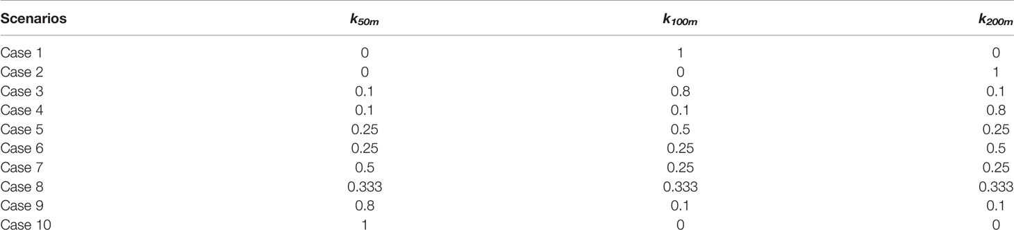
Table 1 Different scenarios for the weights of seawater temperature of different depths.

Assessment of the Impacts of Antarctic Sea Ice on I. argentinus Habitat

To examine the relationship between vertical water temperature and SIE, spatial correlation between sea water temperature at different depths and SIE from January to April in 1979–2017 was initially determined and drawn (Yu et al., 2017).

In addition, the data of sea water temperature at 50, 100, and 200 m from January to April in 1979–2017 were included into the optimal HSI model, which only need to input sea water temperature in different depths to quantify the proportion of suitable habitat (areas with HSI ≥ 0.6) accounting for the fishing ground in the high seas. The relationship between the proportion of suitable habitat and the SIE was evaluated by correlation analysis.

Furthermore, the years with high and low SIE were selected and divided into two groups from 1979 to 2017 (including 1982, 1983, 1987, 2003, 2008, 2013, 2014, and 2015 with the high SIE; 1980, 1984, 1992, 2005, 2006, 2007, 2010, and 2016 with the low SIE). The suitable habitat and the latitudinal gravity centers (LATG) of HSI were calculated and compared between the two year groups (Yu et al., 2016). The boxplot analysis was used to compare the difference between the two year groups. The LATG was calculated using the following equation:

$\begin{array}{ll}LATG=\frac{{\displaystyle \sum \left(LA{T}_{is}\times HS{I}_{is}\right)}}{{\displaystyle \sum HS{I}_{is}}}& (4)\end{array}$

where LAT_is was the latitude within the fishing unit i in month s and HSI_is was the total HSI within the fishing unit i in month s.

Two representative years with the highest and the lowest SIE (2014 and 2017) were specifically selected from each year group. Between the two years, the sea water temperature, SI, HSI, and the optimal temperature isotherm at different water depths for I. argentinus were compared and analyzed. Spatial distribution maps were created to show the habitat characteristics and specific differences between the two years.

Results

Development, Selection, and Validation of the Integrated HSI Model

The SI curves of I. argentinus were all significant (P < 0.05) for each environmental factor with high correlation coefficients from January to April during 2013–2016. The specific fitted curve, corresponding equation, and the statistical assessments of the SI models were referred to Figure 1 and Table 2.

FIGURE 1

Figure 1 Fitted SI curves of water temperature at different depths from January to April.

TABLE 2

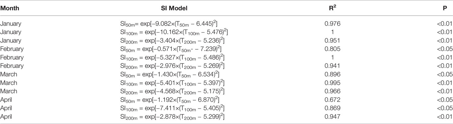
Table 2 Fitting formula of SI models.

With regard to the selection of the optimal HSI model, 10 different weighting-based scenarios were compared one by one, the proportion of fishing effort, catch, and average CPUE were determined. According to the results, the optimal HSI model with the best prediction performance from January to April was case 4 (Tables 3, 4). The weights of water temperature at depths of 50, 100, and 200 m were 0.1, 0.1, and 0.8 (Table 1), respectively, implying that sea water temperature at 200 m contributed most to the habitat variation of I. argentinus. Fisheries data in 2017 were used to validate the optimal HSI model. It showed that high catch, fishing effort, and CPUE were consistent with the high HSI class interval in each month, indicating that this model could effectively predict the potential habitat for I. argentinus (Table 5). Moreover, the spatial distribution maps of HSI and effort in 2013–2016 and 2017 also showed the same results (Figures 2, 3).

TABLE 3

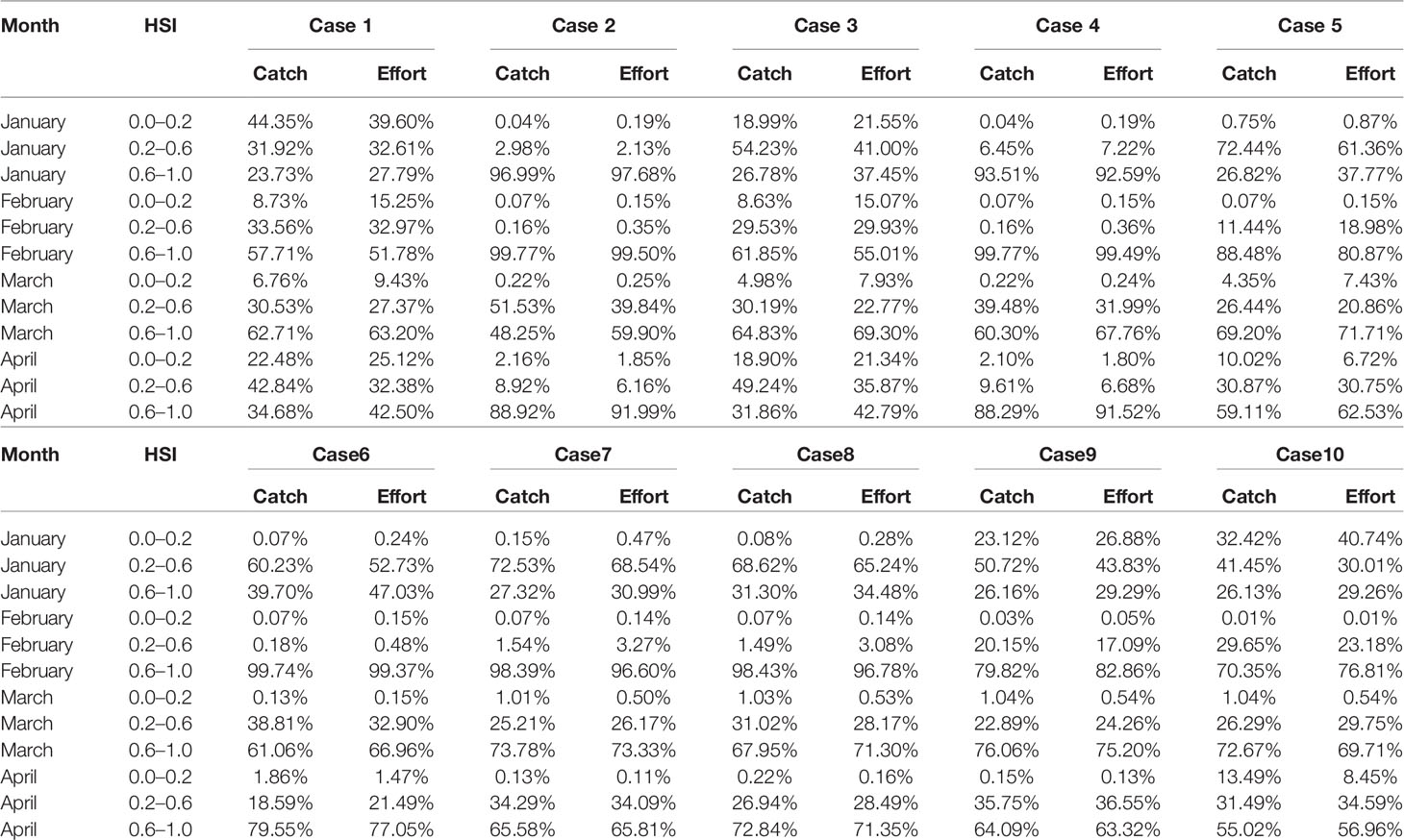
Table 3 Percentage of catch and effort under different HSI class interval sourced from different weighting model during 2013–2016.

TABLE 4

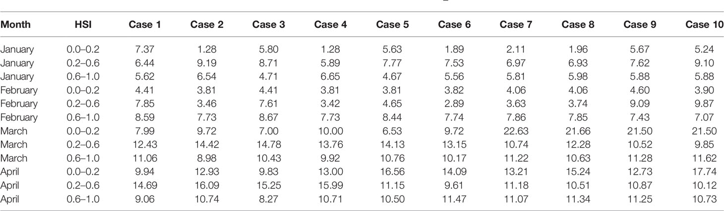
Table 4 CPUE under different HSI class interval sourced from different weighting model during 2013–2016.

TABLE 5

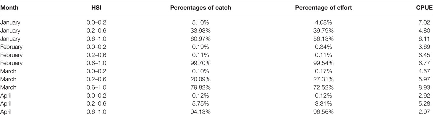
Table 5 Forecast results of comprehensive HSI model in 2017 (the results of validation).

FIGURE 2

Figure 2 Spatial distribution of HSI overlaid with fishing effort from 2013 to 2016.

FIGURE 3

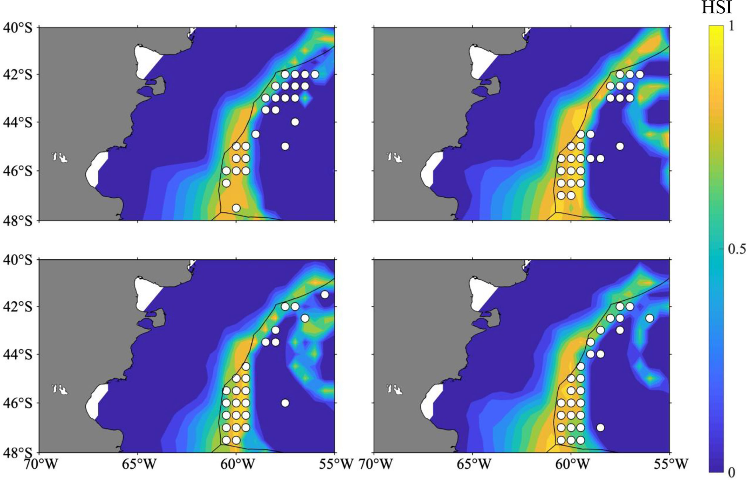
Figure 3 Spatial distribution of HSI overlaid with fishing location in 2017 (the white circle indicates the fishing location) (the results of forecasting).

Impacts of SIE on Water Temperature and Suitable Habitat of I. argentinus

According to the spatial correlation analysis between SIE and sea water temperature at 50, 100, and 200 m on the fishing ground in the high seas of the Southwest Atlantic Ocean from January to April in 1979–2017, SIE was significantly positively correlated with sea water temperature at different depths (Figure 4). Regarding the relationship between the proportions of suitable habitats of I. argentinus and SIE from January to April in 1979–2017, it showed that the proportions of suitable habitats was significantly positively correlated with SIE (r = 0.17, P < 0.05), implying that the larger the SIE, the higher the proportions of suitable habitats (Figure 5).

FIGURE 4

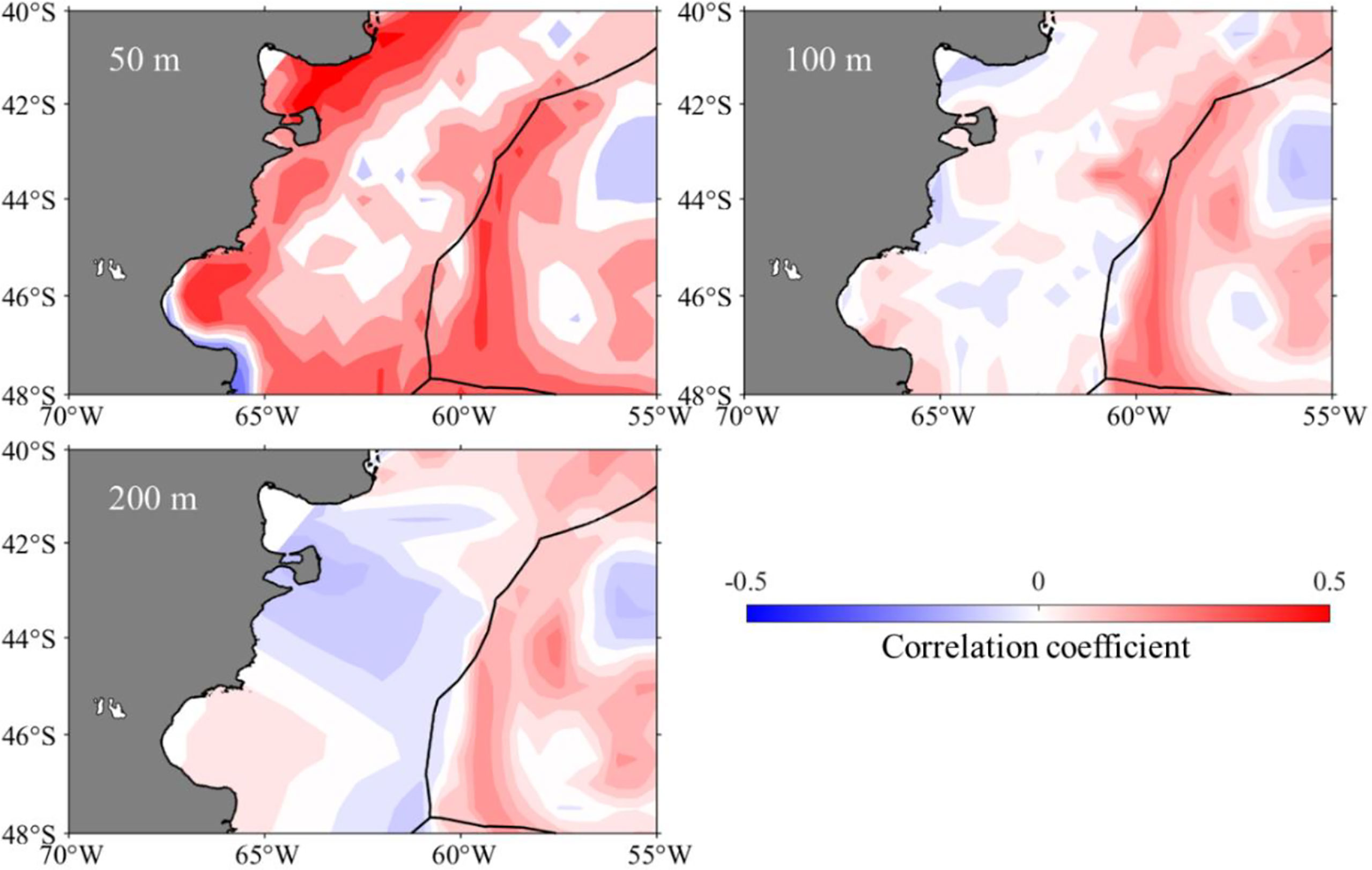
Figure 4 Spatial distribution of correlation coefficient between sea water temperature at depths of 50, 100, and 200 m and sea ice extent from 1979 to 2017 on the fishing ground in the high seas of Southwest Atlantic Ocean.

FIGURE 5

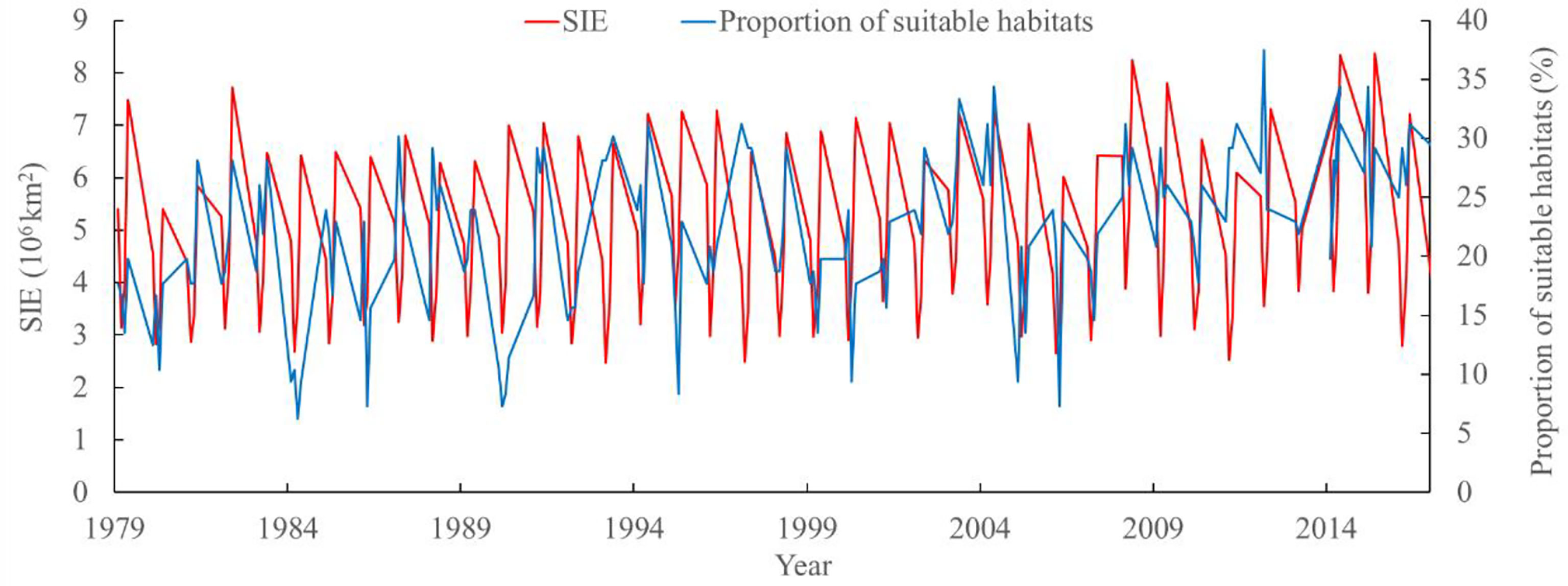
Figure 5 Interannual variability of sea ice extent (SIE) and the proportion of suitable habitat of Illex argentinus from January to April in 1979–2017 on the fishing ground in the high seas of Southwest Atlantic Ocean.

Habitat Pattern Comparison Between the Years With High and Low SIE

According to the annual average SIE, 1979–2017, 1982, 1983, 1987, 2003, 2008, 2013, 2014, an 2015 were the years with the high SIE; 1980, 1984, 1992, 2005, 2006, 2007, 2010, and 2016 were the years with the low SIE. Those years were divided into two year groups with the high and low SIE and compared the difference in habitat pattern including the proportion and latitudinal location of suitable SI_50m (SI_50m ≥0.6), suitable SI_100m (SI_100m ≥ 0.6), suitable SI_200m (SI_200m ≥ 0.6), and suitable habitats of I. argentinus (HSI ≥ 0.6) (Figures 6, 7). It showed that the proportions of abovementioned parameters were higher during the years with high SIE, whereas they were lower in the years with low SIE (Figure 6). Furthermore, latitudinal gravity centers of suitable SI_50m (LATG_SI_50m), suitable SI_100m (LATG_SI_100m), and suitable SI_200m (LATG_SI_200m), and suitable habitats of I. argentinus (LATG_HSI) were distributed in the northern waters on the fishing ground in the years with high SIE, whereas they were located in the southern waters in the years with low SIE (Figure 7).

FIGURE 6

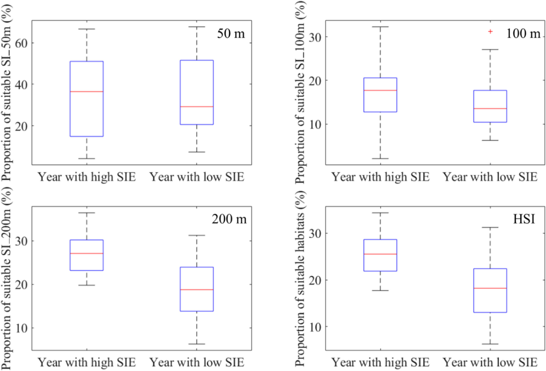
Figure 6 Comparison of the proportion of suitable suitability index for sea water temperature at depths of 50 m (SI_50m ≥ 0.6), 100 m (SI_100m ≥ 0.6), and 200 m (SI_200m ≥ 0.6) and the proportion of suitable habitat (areas with HSI ≥ 0.6) between the year groups with high and low sea ice extent (SIE).

FIGURE 7

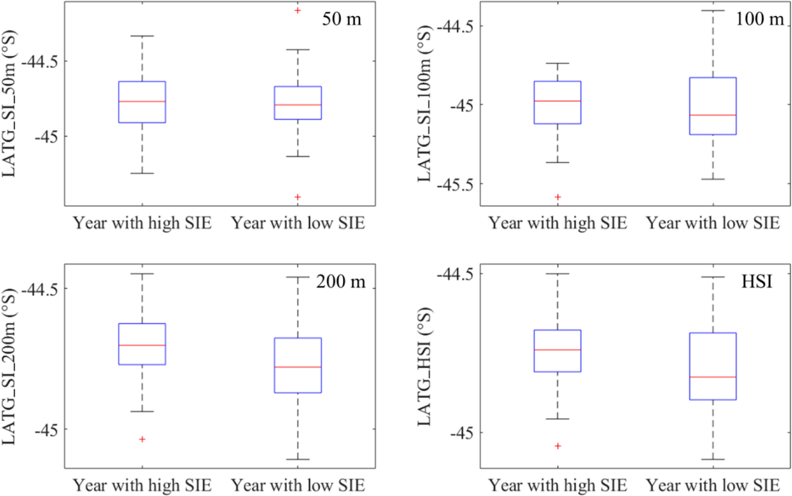
Figure 7 Comparison of the latitudinal gravity centers of suitability index for sea water temperature at depths of 50, 100, and 200 m (LATG_SI_50m, LATG_SI_100m, and LATG_SI_200m) and the latitudinal gravity centers of the integrated habitat suitability index (LATG_HSI) between the year groups with high and low sea ice extent (SIE).

The year 2014 with the highest SIE and year 2017 with the lowest SIE were selected as two representative years corresponding to the year group with high and low SIE, respectively. The spatial distribution for the difference in sea water temperature at various depths illustrated that the water temperature was high on the high-sea fishing ground at different depths. The average water temperature in each month from January to April was higher in 2014 than that in 2017 (Figure 8). Similarly, it was clearly showed that SI values at different water layers were much higher in 2014 than those in 2017 (Figure 9). In addition, the spatial distribution for difference in HSI was consistent with the results of SI comparison; meanwhile, LATG_HSI was located in the northern waters in 2014 comparing to 2017 (Figure 10). On the basis of the fitted formula of the SI model for each environmental factor, the optimum temperature at each water depth from January to April was determined [the b value in formula (2), which was calculated in Table 2]. The isotherms of the most suitable temperature at depths of 50, 100, and 200 m in different months of 2014 and 2017 were drawn in the Southwest Atlantic Ocean (Figure 11). According to the spatial distribution of the isotherms, the most suitable temperature isotherms in 2014 with high SIE moved northward comparing to the year of 2017 with lower SIE. The results indicated that the water temperature at different depths was warmer in 2014 combined with higher SI and HSI, and the isotherm of LATG_HSI and optimum water temperature in each water depth shifted northward.

FIGURE 8

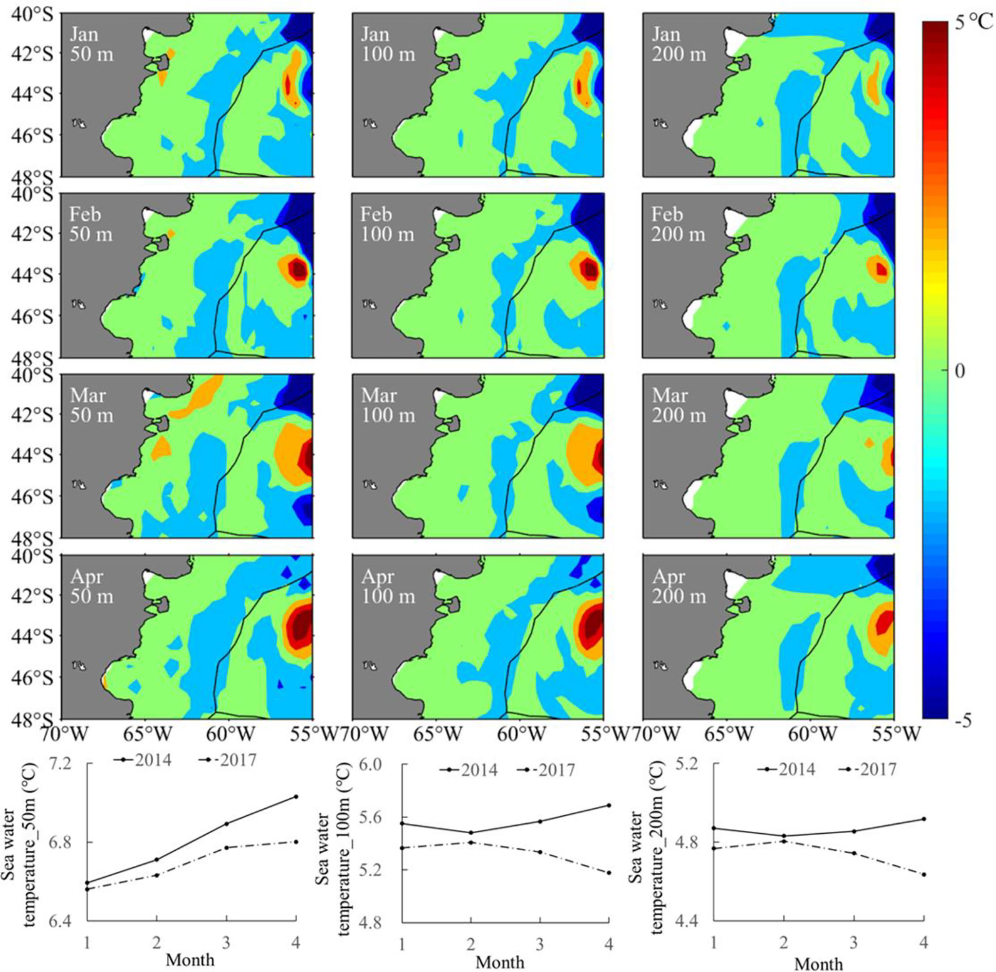
Figure 8 Spatial and temporal difference in sea water temperature (the upper panel) and average sea water temperature (lower panel) from January to April between 2014 and 2017 at depths of 50, 100, and 200 m in the Southwest Atlantic Ocean.

FIGURE 9

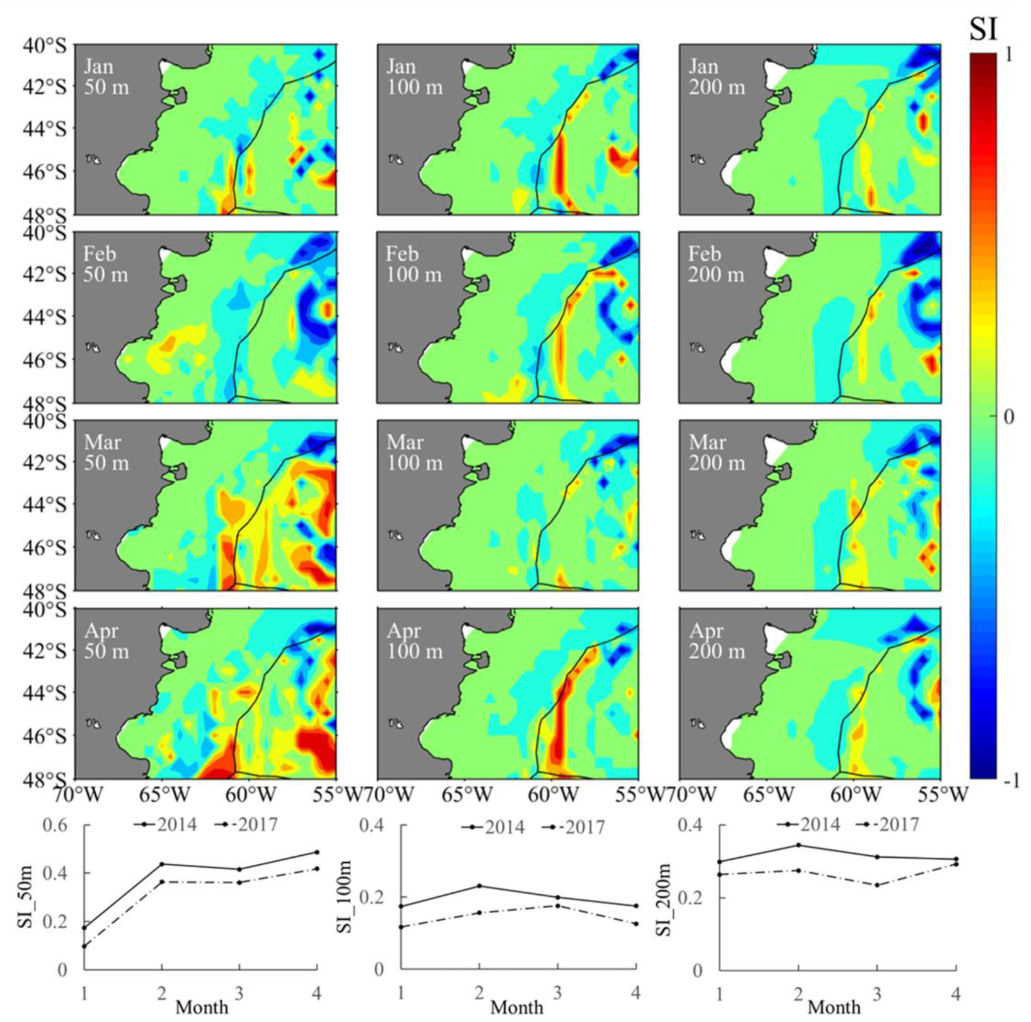
Figure 9 Spatial and temporal difference in suitability index of sea water temperature (the upper panel) and average suitability index of sea water temperature (lower panel) from January to April between 2014 and 2017 at depths of 50, 100, and 200 m in the Southwest Atlantic Ocean.

FIGURE 10

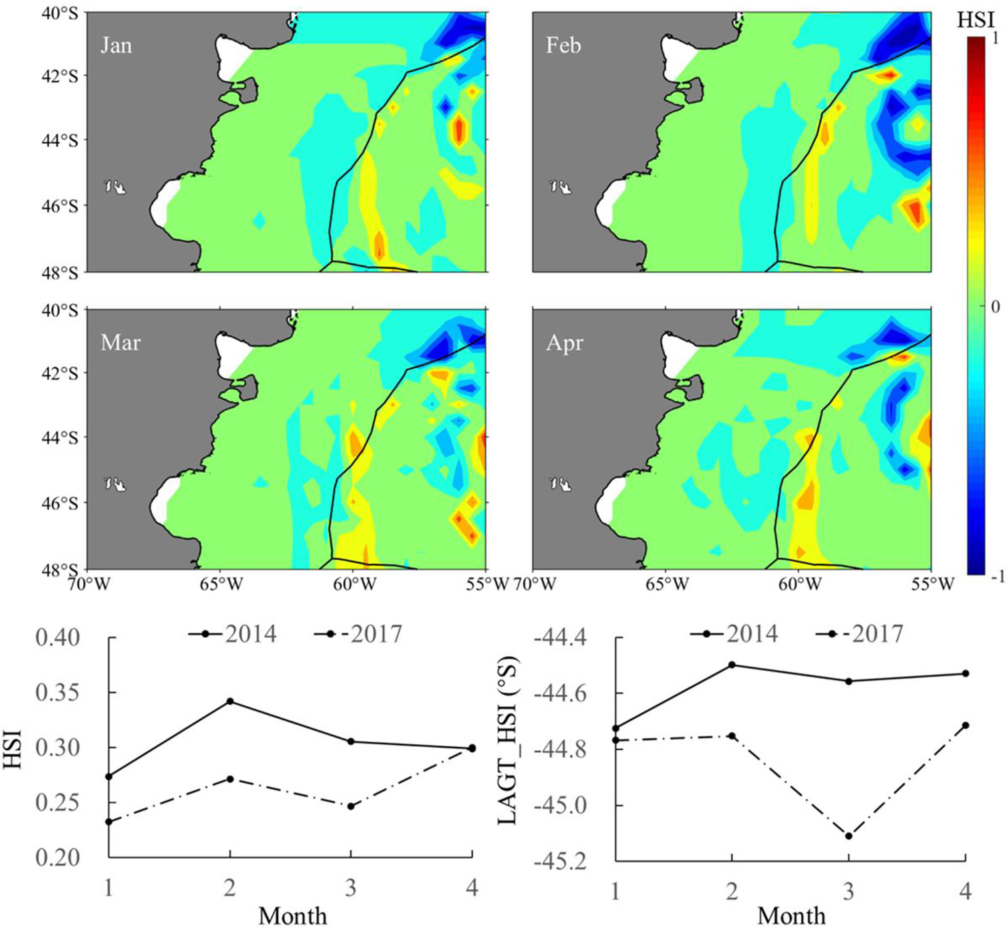
Figure 10 Spatial and temporal difference in habitat suitability index (HSI) (the upper panel) and average HSI and latitudinal gravity centers of HSI (LATG_HSI) (lower panel) from January to April between 2014 and 2017 in the Southwest Atlantic Ocean.

FIGURE 11

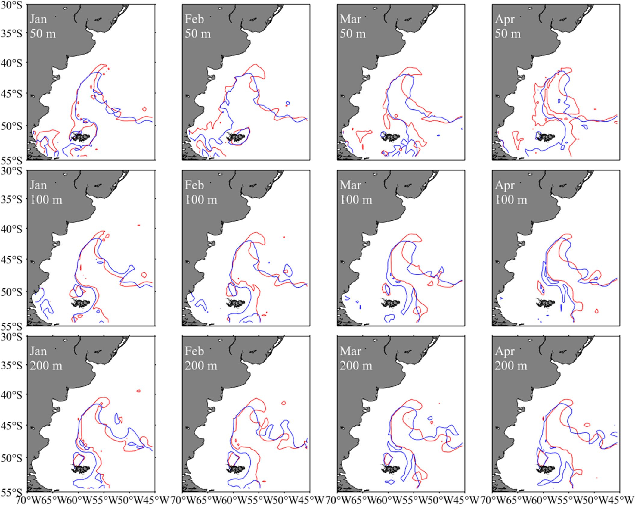
Figure 11 Spatial distribution of optimum temperature isotherms for Illex argentinus at different depths in 2014 and 2017 from January to April (the red line indicated the isotherm in 2014 and the blue line indicated the isotherm in 2017).

Discussion

The Construction of the Integrated HSI Model

The integrated HSI model was established on the basis of the fisheries data combined with sea water temperature at three crucial water layers from 2013 to 2016, and the accuracy and feasibility of the model were validated using the data in 2017. Moreover, according to the consistency in spatial distribution of HSI and fishing effort, the integrated HSI model was realized with satisfactory prediction performance. HSI model was generally applied to describe the relationship between species and their habitats (Hyun et al., 2020). At present, HSI model has been widely used in the detection and prediction of fishing ground based on different environmental factors (Yu et al., 2020). Previous studies suggested that fishing effort was the optimal indicator of species occurrence among fishing effort, catch, and CPUE for squids (Abrahams and Healey, 1993; Rijnsdorp et al., 2000; Swain and Wade, 2003). Therefore, the fishing effort was used to calculate SI value in this study. Compared the HSI model established by two species occurrence indicators, the importance of fishing vessel operation position was highlighted in this study (Chen et al., 2012; Yu et al., 2020). In addition, the prediction performance in January 2017 was relatively poor compared with other months, the reasons might be as follows: (i) the total fishing effort in January was less; (ii) the fishing effort was scattered at the beginning of fishing season; and (iii) January was the transition period of the habitat distribution for I. argentinus from shallow to deep water (Bazzino et al., 2005).

SST, Chla, and SSH were often used as environmental factors to build HSI model. However, most marine organisms including I. argentinus migrated horizontally and vertically day and night during their whole life cycle and inhabited at different water layers (Koronkiewicz, 1986). Therefore, the HSI model based on surface environmental factors was difficult to accurately describe the relationship between the habitat and organisms. Very few studies investigated the correlation between environmental factors at deep water layers and I. argentinus except surface environmental factors. For other squid species such as Ommastrephes bartrammi in the Northwest Pacific Ocean, model prediction performance showed large difference based on surface environmental conditions and vertical water temperature. For example, four surface environmental factors (SST, sea surface salinity, SSH anomaly, and Chla) from August to October in 1999 to 2004 were used to establish HSI models for O. bartramii, and the prediction success rate was 65.17% (Chen et al., 2010). Whereas the prediction accuracy was 82.5% for the HSI model developed by fishing effort as well as SST, vertical structure of water temperature in 0–50 m, and sea water temperature at 200 m and 300 m (Chen et al., 2012). These findings implied that the HSI model should consider sea water temperature at deep-sea layers to obtain a more accurate HSI model.

Influence of Vertical Water Temperature on I. argentinus

According to the optimal HSI model selecting from the 10 weighting scenarios, it illustrated that sea water temperature at 200 m was the most important factor in regulating habitat distribution of I. argentinus. Variability in areas of suitable HSI and its latitudinal location was consistent with suitable SI_200m and its distribution (Figures 6, 7). The difference of proportion of suitable habitats and LATG_HSI for the two year groups with high and low SIE were most obvious at depth of 200 m.

Illex argentinus is a pelagic economic cephalopod with vertical migration behavior (Bazzino et al., 2005). The vertical water temperature will affect the abundance and distribution of fishing ground of I. argentinus (Chen et al., 2012). There were studies suggested that the ratio of temperature difference at different water depth (sea water temperature gradient △t/△d) also played an important role in fish habitat distribution (Song and Zhou, 2010; Chen et al., 2012; Yan et al., 2016). In this study, an integrated HSI model was established on the basis of sea water temperature at different depths. However, inclusive of water temperature gradient in the establishment of HSI model might be more accurate. The results showed that sea water temperature at 200 m contributed the most important influences to I. argentinus habitat. The important relationship between the distribution of I. argentinus and water temperature at 200 m water layers may be related to thermocline (Yatsu and Watanabe, 1996). The formation, rupture, and spatial heterogeneity of the thermocline in different seasons had a significant impact on marine life in Patagonia Gulf in the northern Argentina of the Southwest Atlantic Ocean (Luzenti et al., 2021). Therefore, for the marine species living above the thermocline, it prevented them from entering the deeper water, which was favorable for the formation of a productive fishing ground above the thermocline. On the contrary, for the marine species inhabiting below the thermocline, it was difficult to attract the fish to rise through the thermocline by means of lighting and other trapping methods, which might lead to lower catch (Wang et al., 2019). Thus, the water layer of the upper and lower boundary of thermocline was important for the formation of fishing grounds (Luzenti et al., 2021). At present, there were few studies on the seasonal and interannual changes on the thermocline position on the fishing ground of I. argentinus in the Southwest Atlantic Ocean. The relationship between the thermocline position and the water depth of 200 m should be further explored.

The Response of Habitat Pattern of I. argentinus to Sea Ice Change

Antarctic sea ice change impacts global biology and environment. Antarctic Circumpolar Wave (ACW) (White and Peterson, 1996) and Antarctic dipole (ADP) (Yuan and Martinson, 2000) induced by Antarctic sea ice will lead to global large-scale climate variability. With the Antarctic sea ice change-driven global climate change as well as the changing ocean salinity structure, the thermohaline in the oceans will significantly change and yield a huge impact on the distribution and migration of marine species (Shin et al., 2003). In this study, SIE was used as an environmental parameter to indicate the change of Antarctic sea ice; sometimes, sea ice area and SIC have been used as indicators to describe the change condition of Antarctic sea ice (Ma et al., 2004; Dai et al., 2012). To explore the impacts of Antarctic sea ice on the organisms outside the sea ice extend area, we can use the SIE or some other indicators as a bridge to connect the Antarctic Ocean with the marine species in the adjacent waters. For instance, the northern boundary of Antarctic sea ice (Ma et al., 2004) and the Antarctic Sea Ice Oscillation Index (Cheng et al., 2002) were used as parameters to indicate the change of Antarctic sea ice to explore the impact on the oceanic environment outside the Antarctic continent. Sea ice distribution of the Indian Ocean, Atlantic Ocean, and Pacific Ocean was estimated on the basis of the quantitative study of diatoms and radiolarians (Gersonde et al., 2005).

In this study, the spatial correlation coefficients between SIE and sea water temperature at different depths were determined to explore the relationship between them in the high-sea fishing ground (Figure 4). The results showed that SIE was positively correlated with sea water temperature at different depths in the main fishing ground of I. argentinus in the Southwest Atlantic Ocean. Moreover, overviewing the whole Southwest Atlantic Ocean at 100- and 200-m water layers, the influence mechanism of SIE on BC and MC was different, and the SIE was negatively correlated with BC in the northern waters and positively correlated with MC in the southern waters near the entrance of La Plata-Parana River. It was speculated that global warming would lead to the melting of Antarctic sea ice and consequently the decreasing of SIE. The sea waters of MC in the south were affected by the deep cold waters because of the melting sea ice, whereas the northern BC was less affected by the sea ice melting. Therefore, the correlation between the sea water temperature and SIE was different in the northern and southern regions. Further analysis should be performed to explore the specific reasons why the cold and warm currents in different directions were affected by Antarctic sea ice in different ways. Antarctic sea ice was characterized by large interannual variability and an increase in areal coverage since 1979 (Eisenman et al., 2014; Comiso et al., 2017) despite an abrupt reduction in SIE since 2016. It may be the turning point of maintaining low SIE (Ludescher et al., 2018), moreover, the influences of the sustaining low SIE to I. argentinus required continuous observation and study.

Except Antarctic sea ice, because of the increase of carbon dioxide emissions and human-induced global warming, the global climate was undergoing dramatic changes, which affected short-lived cephalopods. For example, the North Atlantic Oscillation dramatically affected Illex illebrosus inhabiting in the North Atlantic Ocean (Dawe et al., 2000), whereas the Antarctic Oscillation (AAO) (Chang et al., 2015) and the Southern Oscillation (Chen et al., 2007) led to the lag of resource change for I. argentinus. In addition, SST anomalies associated with the El Niño events in the Pacific Ocean propagated around the globe via ACW; thus, predicting anomalous oceanic events via teleconnections between SST anomalies in the Pacific and Atlantic Ocean would appear to have the potential to predict the recruitment strength of I. argentinus in the Southwest Atlantic Ocean (Waluda et al., 1999). The relationship between the environment of the Southern Ocean and cephalopods living near the Antarctic continent has also been explored; ocean acidification may have a greater impact on cephalopods (Rodhouse, 2013; Constable et al., 2014; Xavier et al., 2016), especially affecting the hatching rate of cephalopods in summer (Rosa et al., 2014). The expansion of the cold waters in the Southern Ocean will increase the carbon absorption capacity (Bakker et al., 1997) with the declined exchange of carbon dioxide between the atmosphere and ocean (Stephens and Keeling, 2000), resulting in the enhancement of ocean acidity.

Conclusion

Overall, conclusions in this study included the following: (i) the integrated HSI model could effectively predict the habitat of I. argentinus; (ii) sea water temperature at depths of 200 m was the most critical factors for the habitat formation of I. argentinus among the depths of 50, 100, and 200 m; (iii) SIE was significantly positively correlated with sea water temperature at different depths and the proportions of suitable habitats; and (iv) the suitable habitats of I. argentinus were located in the southern waters in the years with lower SIE. Furthermore, the melting Antarctic sea ice is yielding adverse effects on I. argentinus habitat in the Southwest Atlantic Ocean by changing the sea water temperature at critical depths. Exploring the relationship between the habitat pattern of I. argentinus and Antarctic sea ice can provide scientific basis for the management and rational utilization of resources and important implications for distant-water squid fisheries.

Data Availability Statement

The original contributions presented in the study are included in the article/supplementary material, further inquiries can be directed to the corresponding author.

Author Contributions

WY and HL conceptualized the study. WY and HL designed the methodology, provided the software, and analyzed the data for the study. WY and HL wrote the original draft. WY involved in the funding acquisition. The manuscript was written through contributions of all authors. All authors contributed to the article and approved the submitted version.

Conflict of Interest

The authors declare that the research was conducted in the absence of any commercial or financial relationships that could be construed as a potential conflict of interest.

Publisher’s Note

All claims expressed in this article are solely those of the authors and do not necessarily represent those of their affiliated organizations, or those of the publisher, the editors and the reviewers. Any product that may be evaluated in this article, or claim that may be made by its manufacturer, is not guaranteed or endorsed by the publisher.

Acknowledgments

This study was financially supported by the National Key R&D Program of China (2019YFD0901405), National Natural Science Foundation of China (41906073), the project of Shanghai talent development funding (2021078), and the open fund of State Key Laboratory of Satellite Ocean Environment Dynamics, Second Institute of Oceanography (QNHX2232).

References

Abrahams M. V., Healey M. C. (1993). Some Consequences of Variation in Vessel Density: A Manipulative Field Experiment. Fish. Res. 15 (4), 315–322. doi: 10.1016/0165-7836(93)90082-I

CrossRef Full Text | Google Scholar

Arkhipkin A. I., Gras M., Blake A. (2015). Water Density Pathways for Shelf/Slope Migrations of Squid Illex Argentinus in the Southwest Atlantic. Fish. Res. 172, 234–242. doi: 10.1016/j.fishres.2015.07.023

CrossRef Full Text | Google Scholar

Armour K. C., Marshall J., Scott J. R., Donohoe A., Newsom E. R. (2016). Southern Ocean Warming Delayed by Circumpolar Upwelling and Equatorward Transport. Nat. Geosci. 9, 549–554. doi: 10.1038/ngeo2731

CrossRef Full Text | Google Scholar

Bakker D. C. E., De-Baar H. J. W., Bathmann U. V. (1997). Changes of Carbon Dioxide in Surface Waters During Spring in the Southern Ocean. Deep-Sea. Res. Pt. II. 44 (1-2), 91–127. doi: 10.1016/S0967-0645(96)00075-6

CrossRef Full Text | Google Scholar

Bazzino G., Quiñones R. A., Norbis W. (2005). Environmental Associations of Shortfin Squid Illex Argentinus (Cephalopoda: Ommastrephidae) in the Northern Patagonian Shelf. Fish. Res. 76 (3), 401–416. doi: 10.1016/j.fishres.2005.07.005

CrossRef Full Text | Google Scholar

Brown S. K., Buja K. R., Jury S. H., Monaco M. E., Banner A. (2000). Habitat Suitability Index Models for Eight Fish and Invertebrate Species in Casco and Sheepscot Bays, Maine. N. Am. J. Fish. Manage. 20 (2), 408–435. doi: 10.1577/1548-8675(2000)0202.3.CO;2

CrossRef Full Text | Google Scholar

Brunetti N. E., Elena B., Rossi G. R., Ivanovic M. L., Aubone A., Guerrero H., et al. (1998). Summer Distribution, Abundance and Population Structure of Illex Argentinus on the Argentine Shelf in Relation to Environmental Features. Afr. J. Mar. Sci. 20s (1), 175–186. doi: 10.2989/025776198784126386

CrossRef Full Text | Google Scholar

Brunetti N. E., Ivanovic M. L., Louge E., Christiansen H. E. (1991). Reproductive Biology and Fecundity of Two Stocks of the Squid (Illex Argentinus). Frente. Marítimo. 8, 73–84.

Google Scholar

Cao J., Chen X., Chen Y. (2009). Influence of Surface Oceanographic Variability on Abundance of the Western Winter-Spring Cohort of Neon Flying Squid Ommastrephes Bartramii in the NW Pacific Ocean. Mar. Ecol. Prog. Ser. 381, 119–127. doi: 10.3354/meps07969

CrossRef Full Text | Google Scholar

Chang K. Y., Chen C. S., Wang H. Y., Kuo C. L., Chiu T. S. (2015). The Antarctic Oscillation Index as an Environmental Parameter for Predicting Catches of the Argentine Shortfin Squid (Illex Argentinus Cephalopoda: Ommastrephidae) in Southwest Atlantic Waters. Fish. B-NOAA. 113 (2), 202–212. doi: 10.7755/FB.113.2.8

CrossRef Full Text | Google Scholar

Chen P., Chen X. J. (2016). Analysis of Habitat Distribution of Argentine Shortfin Squid (Illex Argentinus) in the Southwest Atlantic Ocean Using Maximum Entropy Model. J. Fish. China 40 (6), 893–902. doi: 10.11964/jfc.20150509873

CrossRef Full Text | Google Scholar

Chen F., Chen X. J., Liu B. L., Qian W. G., Tian S. Q. (2010). Relationship Between Fishing Ground of Ommastrephes Bartramii and Vertical Temperature Structure in the Northwestern Pacific Ocean. J. Shanghai. Ocean. Univ. 19 (04), 495–504. doi: 10.3724/SP.J.1231.2010.06781

CrossRef Full Text | Google Scholar

Cheng Y. J., Bian L. G., Lu L. H. (2002). Antarctic Sea-Ice Oscillation and its Relationship With ENSO. J. App. Meteor. Sci. 13 (6), 711–717. doi: 10.3969/j.issn.1001-7313.2002.06.009

CrossRef Full Text | Google Scholar

Chen C. S., Haung W. B., Chiu T. S. (2007). Different Spatiotemporal Distribution of Argentine Short-Finned Squid (Illex Argentinus) in the Southwest Atlantic During High-Abundance Year and its Relationship to Sea Water Temperature Changes. Zool. Stud. 46 (3), 362–374.

Google Scholar

Chen X. J., Lu H. J., Liu B. L., Qian W. G. (2012). Forecasting Fishing Ground of Illex Argentinus by Using Habitat Suitability Model in the Southwest Atlantic. J. Shanghai. Ocean. Univ. 21 (3), 431–438. doi: 10.1007/s11783-011-0280-z

CrossRef Full Text | Google Scholar

Chiu T. Y., Chiu T. S., Chen C. S. (2017). Movement Patterns Determine the Availability of Argentine Shortfin Squid Illex Argentinus to Fisheries. Fish. Res. 193, 71–80. doi: 10.1016/j.fishres.2017.03.023

CrossRef Full Text | Google Scholar

Comiso J. C., Gersten R. A., Stock L. V., Turner J., Perez G. J., Cho K. (2017). Positive Trend in the Antarctic Sea Ice Cover and Associated Changes in Surface Temperature. J. Climate. 30, 2251–2267. doi: 10.1175/JCLI-D-16-0408.1

CrossRef Full Text | Google Scholar

Constable A. J., Melbourne-Thomas J., Corney S. P., Arrigo K. R., Babraud C., Barnes D. K. A., et al. (2014). Climate Change and Southern Ocean Ecosystems I: How Changes in Physical Habitats Directly Affect Marine Biota. Global Change Biol. 20 (10), 3004–3025. doi: 10.1111/gcb.12623

CrossRef Full Text | Google Scholar

Dai L. F., Zhang S. M., Fan W. (2012). The Abundance Index of Antarctic Krill and its Relationship to Sea Ice and Sea Surface Temperature. Chin. J. Pol. Res. 24 (4), 352–360. doi: 10.3724/SP.J.1084.2012.00352

CrossRef Full Text | Google Scholar

Dawe E. G., Colbourne E. B., Drinkwater K. F. (2000). Environmental Effects on Recruitment of Short-Finned Squid (Illex Illecebrosus). ICES. J. Mar. Sci. 57 (4), 1002–1013. doi: 10.1006/jmsc.2000.0585

CrossRef Full Text | Google Scholar

Eisenman I., Meier W. N., Norris J. R. (2014). A Spurious Jump in the Satellite Record: Has Antarctic Sea Ice Expansion Been Overestimated? Cryosphere 8, 1289–1296. doi: 10.5194/tc-8-1289-2014

CrossRef Full Text | Google Scholar

Fedulov P. P., Remeslo A. V., Burykin S. N. (1990). Variabilidad De La Corriente De Malvinas. Frente. Marítimo. 6, 121–130. doi: 10.1038/141800a0

CrossRef Full Text | Google Scholar

FAO. (2017 ). Food and Agriculture Organization of the United Nations. Food and Agriculture Organization of the United Nations’ Fisheries Database: Global Production Statistics 1950-2017. Available at: http://www.fao.org/fishery/statistics/global-production/query/en.

Google Scholar

Friocourt Y., Drijfhout S., Blanke B., Sabrina S. (2005). Water Mass Export From Drake Passage to the Atlantic, Indian, and Pacific Oceans: A Lagrangian Model Analysis. J. Phys. Oceanogr. 35 (7), 1206–1222. doi: 10.1175/JPO2748.1

CrossRef Full Text | Google Scholar

Gersonde R., Crosta X., Abelmann A., Armand L. (2005). Sea-Surface Temperature and Sea Ice Distribution of the Southern Ocean at the EPILOG Last Glacial Maximum—a Circum-Antarctic View Based on Siliceous Microfossil Records. Quater. Sci. Rev. 24 (7–9), 869–896. doi: 10.1016/j.quascirev.2004.07.015

CrossRef Full Text | Google Scholar

Hobbs W. R., Massom R., Stammerjohn S., Reid P., Williams G., Meier W. (2016). A Review of Recent Changes in Southern Ocean Sea Ice, Their Drivers and Forcings. Global Planet. Change. 143, 228–250. doi: 10.1016/j.gloplacha.2016.06.008

CrossRef Full Text | Google Scholar

Hyun J. K., Joong H. K., Un J., Sang H. J. (2020). Effect of Probability Distribution-Based Physical Habitat Suitability Index on Environmental-Flow Estimation. KSCE. J. Civ. Eng. 24 (8), 2393–2402. doi: 10.1007/s12205-020-1923-z

CrossRef Full Text | Google Scholar

Koronkiewicz (1986). Growth and Life Cycle of Squid Illex Argentinus From (the) Patagonian and Falkland Shelf and Polish Fishery of Squid for This Region: 1978–1985. ICES. Council. Meet. Pap. 27, 1–16.

Google Scholar

Legeckis R., Gordon A. L. (1982). Satellite Observations of the Brazil and Falkland Currents—1975 1976 and 1978. Deep-Sea. Res. Pt. I. 29 (3), 375–401. doi: 10.1016/0198-0149(82)90101-7

CrossRef Full Text | Google Scholar

Li G., Chen X. J., Lei L., Guan W. J. (2014). Distribution of Hotspots of Chub Mackerel Based on Remote-Sensing Data in Coastal Waters of China. Int. J. Remote Sens. 35, 4399–4421. doi: 10.1080/01431161.2014.916057

CrossRef Full Text | Google Scholar

Liu H. W., Yu W., Chen X. J. (2020). A Review of Illex Argentinus Resources and the Responses to Environmental Variability in the Southwest Atlantic Ocean. J. Fish. Sci. China. 27 (10), 1254–1265. doi: 10.3724/SP.J.1118.2020.20056

CrossRef Full Text | Google Scholar

Liu H. W., Yu W., Chen X. J., Wang J. T., Zhang Z. (2021). Influence of Antarctic Sea Ice Variation on Abundance and Spatial Distribution of Argentine Shortfin Squid Illex Argentinus in the Southwest Atlantic Ocean. J. Fish. China. 45 (2), 187–199. doi: 10.11964/jfc.20191112074

CrossRef Full Text | Google Scholar

Ludescher J., Yuan N. M., Bunde A. (2018). Detecting the Statistical Significance of the Trends in the Antarctic Sea Ice Extent: An Indication for a Turning Point. Clim. Dynam. 53 (5), 237–244. doi: 10.1007/s00382-018-4579-3

CrossRef Full Text | Google Scholar

Luzenti E. A., Svendsen G. M., Degrati M., Nadia S. C., Raul A. G., Silvana L. D. (2021). Physical and Biological Drivers of Pelagic Fish Distribution at High Spatial Resolution in Two Patagonian Gulfs. Fish. Oceanogr. 00, 1–16. doi: 10.1111/fog.12526

CrossRef Full Text | Google Scholar

Ma L. J., Lu L. H., Bian L. G. (2004). Spatio-Temporal Character of Antarctic Sea Ice Variation. Chin. J. Pol. Res. 16 (1), 29–37. doi: 10.1007/BF02873097

CrossRef Full Text | Google Scholar

Massom R. A., Stammerjohn S. E. (2010). Antarctic Sea Ice Change and Variability–Physical and Ecological Implications. Pol. Sci. 4 (2), 149–186. doi: 10.1016/j.polar.2010.05.001

CrossRef Full Text | Google Scholar

Meehl G. A., Arblaster J. M., Chung C. T., Holland M. M., DuVivier A., Thompson L., et al. (2019). Sustained Ocean Changes Contributed to Sudden Antarctic Sea Ice Retreat in Late 2016. Nat. Community 10, 14. doi: 10.1038/s41467-018-07865-9

CrossRef Full Text | Google Scholar

National Snow & Ice Data Center (NSIDC). Available at: https://nsidc.org/data/seaice_index/.

Google Scholar

Olson D. B., Podestá G. P., Evans R. H., Brown O. (1988). Temporal Variations in the Separation of Brazil and Malvinas Currents. Deep-Sea. Res. Pt. I. 35 (12), 1971–1990. doi: 10.1016/0198-0149(88)90120-3

CrossRef Full Text | Google Scholar

Purich A., England M. H. (2019). Tropical Teleconnections to Antarctic Sea Ice During Austral Spring 2016 in Coupled Pacemaker Experiments. Geophys. Res. Lett. 46, 6848–6858. doi: 10.1029/2019GL082671

CrossRef Full Text | Google Scholar

Queirós J. P., Phillips R. A., Baeta A., Abreu J., Xavier J. C. (2019). Habitat, Trophic Levels and Migration Patterns of the Short-Finned Squid Illex Argentinus From Stable Isotope Analysis of Beak Regions. Pol. Biol. 42 (12), 2299–2304. doi: 10.1007/s00300-019-02598-x

CrossRef Full Text | Google Scholar

Rijnsdorp A. D., Dol W., Hoyer M., Pastoors M. A. (2000). Effects of Fishing Power and Competitive Interactions Among Vessels on the Effort Allocation on the Trip Level of the Dutch Beam Trawl Fleet. ICES. J. Mar. Sci. 57 (4), 927–937. doi: 10.1006/jmsc.2000.0580

CrossRef Full Text | Google Scholar

Rodhouse P. G. K. (2013). Role of Squid in the Southern Ocean Pelagic Ecosystem and the Possible Consequences of Climate Change. Deep-Sea. Res. Pt. II. 95, 129–138. doi: 10.1016/j.dsr2.2012.07.001

CrossRef Full Text | Google Scholar

Rosa R., Trubenbach K., Pimentel M. S., Boavida-Portugal J., Faleiro F., Baptista M., et al. (2014). Differential Impacts of Ocean Acidification and Warming on Winter and Summer Progeny of a Coastal Squid (Loligo Vulgaris). J. Exp. Biol. 217 (4), 518–525. doi: 10.1242/jeb.096081

PubMed Abstract | CrossRef Full Text | Google Scholar

Sacau M., Pierce G. J., Wang J. J., Arkhipkin A. I., Portela J., Brickle P., et al. (2005). The Spatio-Temporal Pattern of Argentine Shortfin Squid Illex Argentinus Abundance in the Southwest Atlantic. Aquat. Liv. Resour. 18 (4), 361–372. doi: 10.1051/alr:2005039

CrossRef Full Text | Google Scholar

Schlosser E., Haumann F. A., Raphael M. N. (2018). Atmospheric Influences on the Anomalous 2016 Antarctic Sea Ice Decay. Cryosphere 12, 1103–1119. doi: 10.5194/tc-12-1103-2018

CrossRef Full Text | Google Scholar

Shin S. I., Liu Z. Y., Otto-Bliesner B. L., Kutzbach J. E., Vavrus S. J. (2003). Southern Ocean Sea-Ice Control of the Glacial North Atlantic Thermohaline Circulation. Geophys. Res. Lett. 30 (2), 1096. doi: 10.1029/2002GL015513

CrossRef Full Text | Google Scholar

Song L. M., Zhou Y. Q. (2010). Developing an Integrated Habitat Index for Bigeye Tuna (Thunnus Obesus) in the Indian Ocean Based on Longline Fisheries Data. Fish. Res. 105 (2), 63–74. doi: 10.1016/j.fishres.2010.03.004

CrossRef Full Text | Google Scholar

Stephens B. B., Keeling R. F. (2000). The Influence of Antarctic Sea Ice on Glacial–Interglacial CO2 Variations. Nature 404 (6774), 171–174. doi: 10.1038/35004556

PubMed Abstract | CrossRef Full Text | Google Scholar

Stroeve J., Holland M. M., Meir W., Scambos T., Serreze M. (2007). Arctic Sea Ice Decline: Faster Than Forecast. Geophys. Res. Lett. 34, L09501. doi: 10.1029/2007GL029703

CrossRef Full Text | Google Scholar

Stuecker M. F., Bitz C. M., Armour K. C. (2017). Conditions Leading to the Unprecedented Low Antarctic Sea Ice Extent During the 2016 Austral Spring Season. Geophys. Res. Lett. 44, 9008–9019. doi: 10.1002/2017GL074691

CrossRef Full Text | Google Scholar

Swain D. P., Wade E. J. (2003). Spatial Distribution of Catch and Effort in a Fishery for Snow Crab (Chionoecetes Opilio): Tests of Predictions of the Ideal Free Distribution. Can. J. Fish. Aquat. Sci. 60 (8), 897–909. doi: 10.1139/f03-076

CrossRef Full Text | Google Scholar

Thompson D. W., Solomon S. (2002). Interpretation of Recent Southern Hemisphere Climate Change. Science 296, 895–899. doi: 10.1126/science.1069270

PubMed Abstract | CrossRef Full Text | Google Scholar

Tian S. Q., Chen X. J., Chen Y., Xu L. X., Dai X. J. (2009). Evaluating Habitat Suitability Indices Derived From Cpue and Fishing Effort Data for Ommatrephes Bartramii in the Northwestern Pacific Ocean. Fish. Res. 95, 181–188. doi: 10.1016/j.fishres.2008.08.012

CrossRef Full Text | Google Scholar

Turner J., Co-Authors (2009). Non-Annular Atmospheric Circulation Change Induced by Stratospheric Ozone Depletion and its Role in the Recent Increase of Antarctic Sea Ice Extent. Geophys. Res. Lett. 36, L08502. doi: 10.1029/2009gl037524

CrossRef Full Text | Google Scholar

Waluda C. M., Trathan P. N., Rodhouse P. G. (1999). Influence of Oceanographic Variability on Recruitment in the Illex Argentinus (Cephalopoda:Ommastrephidae) Fishery in the South Atlantic. Mar. Ecol. Prog. Ser. 183, 159–167. doi: 10.3354/meps183159

CrossRef Full Text | Google Scholar

Wang Y. G., Chen X. J. (2005). Resources and Fisheries of the Economic Oceanic Squid in the World (Beijing: China Ocean Press), 240–264.

Google Scholar

Wang J. T., Chen X. J., Chen Y. (2018). Projecting Distributions of Argentine Shortfin Squid (Illex Argentinus) in the Southwest Atlantic Using a Complex Integrated Model. Acta Oceanol. Sin. 37 (8), 31–37. doi: 10.1007/s13131-018-1231-3

CrossRef Full Text | Google Scholar

Wang L. M., Li Y., Zhang R., Tian Y. J., Zhang J., Lin L. S. (2019). Relationship Between the Resource Distribution of Scomber Japonicus and Seawater Temperature Vertical Structure of Northwestern Pacific Ocean. Period. Ocean. U. China. 49 (11), 29–38. doi: 10.16441/j.cnki.hdxb.20180174

CrossRef Full Text | Google Scholar

White B. W., Peterson R. G. (1996). An Antarctic Circumpolar Wave in Surface Pressure, Wind, Temperature and Sea-Ice Extent. Nature 380 (6576), 699–702. doi: 10.1038/380699a0

CrossRef Full Text | Google Scholar

Xavier J. C., Raymond B., Jones D. C., Griffiths H. J. (2016). Biogeography of Cephalopods in the Southern Ocean Using Habitat Suitability Prediction Models. Ecosystems 19 (2), 220–247. doi: 10.1007/s10021-015-9926-1

CrossRef Full Text | Google Scholar

Yan L., Zhang P., Yang B. Z., Chen S., Li Y. N., Li Y., et al. (2016). Relationship Between the Catch of Symplectoteuthis Oualaniensis and Surface Temperature and the Vertical Temperature Structure in the South China Sea. J. Fish. Sci. China. 42 (06), 52–60. doi: 10.3724/SP.J.1118.2016.15134

CrossRef Full Text | Google Scholar

Yatsu A., Watanabe T. (1996). Interannual Variability in Neon Flying Squid Abundance and Oceanographic Conditions in the Central North Pacific 1982-1992. Bull. Natl. Res. Inst. Far. Seas. Fish. 33, 123–138. doi: 10.1021/acs.cgd.8b00266

CrossRef Full Text | Google Scholar

Yuan X. J., Martinson D. G. (2000). Antarctic Sea Ice Extent Variability and its Global Connectivity. J. Climate. 13 (10), 1699–1717. doi: 10.1175/1520-0442(2000)0132.0.CO;2

CrossRef Full Text | Google Scholar

Yu W., Chen X., Yi Q., Chen Y. (2016). Spatio-Temporal Distributions and Habitat Hotspots of the Winter-Spring Cohort of Neon Flying Squid Ommastrephes Bartramii in Relation to Oceanographic Conditions in the Northwest Pacific Ocean. Fish. Res. 175, 103–115. doi: 10.1016/j.fishres.2015.11.026

CrossRef Full Text | Google Scholar

Yu W., Chen X., Zhang Y., Yi Q. (2019). Habitat Suitability Modelling Revealing Environmental-Driven Abundance Variability and Geographical Distribution Shift of Winter-Spring Cohort of Neon Flying Squid Ommastrephes Bartramii in the Northwest Pacific Ocean. ICES. J. Mar. Sci. 76 (6), 1722–1735. doi: 10.1093/icesjms/fsz051

CrossRef Full Text | Google Scholar

Yu W., Guo A., Zhang Y., Chen X. J., Qian W. G., Li Y. S. (2018). Climate-Induced Habitat Suitability Variations of Chub Mackerel, Scomber Japonicus, in the East China Sea. Fish. Res. 207, 63–73. doi: 10.1016/j.fishres.2018.06.007

CrossRef Full Text | Google Scholar

Yu W., Wen J., Zhang Z., Chen X. J., Zhang Y. (2020). Spatio-Temporal Variations in the Potential Habitat of a Pelagic Commercial Squid. J. Mar. Syst. 206, 103339. doi: 10.1016/j.jmarsys.2020.103339

CrossRef Full Text | Google Scholar

Yu W., Yi Q., Chen X. J., Chen Y. (2017). Climate-Driven Latitudinal Shift in Fishing Ground of Jumbo Flying Squid (Dosidicus Gigas) in the Southeast Pacific Ocean Off Peru. Int. J. Remote Sens. 38 (12), 3531–3550. doi: 10.1080/01431161.2017.1297547

CrossRef Full Text | Google Scholar

Zhang L., Delworth T. L., Cooke W., Yang X. (2019). Natural Variability of Southern Ocean Convection as a Driver of Observed Climate Trends. Nat. Clim. Change. 9, 59–65. doi: 10.1038/s41558-018-0350-3

CrossRef Full Text | Google Scholar

Zhang L., Gan B. L., Li X. C., Wang H., Wang C. Y., Cai W. J., et al. (2021). Remote Influence of the Midlatitude South Atlantic Variability in Spring on Antarctic Summer Sea Ice. Geophys. Res. Lett. 48, e2020GL090810. doi: 10.1029/2020GL090810

CrossRef Full Text | Google Scholar