 Chao-Yang Kuo1
 Cheng-Han Tsai2
 Ya-Yi Huang1
 Wei Khang Heng1
 An-Tzi Hsiao3Hernyi Justin Hsieh4
 Chaolun Allen Chen1,5,6*
- 1Biodiversity Research Center, Academia Sinica, Taipei, Taiwan
- 2College of Science and Engineering, James Cook University, Townsville, QLD, Australia
- 3Department of Biological Science and Technology, National Yang Ming Chiao Tung University, Hsinchu, Taiwan
- 4Penghu Marine Biology Research Center, Fisheries Research Institute, Council of Agriculture, Makung, Taiwan
- 5Department of Life Science, National Taiwan Normal University, Taipei, Taiwan
- 6Department of Life Science, Tunghai University, Taichung, Taiwan
The Point Intercept Transect (PIT) method has commonly been used in recent decades for estimating the status of coral reef benthic communities. It is a simple method that is efficiently performed underwater, as benthic components are recorded only as presence or absence at specific interval points along transects. Therefore, PIT is also popular in citizen science activities such as Reef Check programs. Longer intervals are commonly associated with longer transects, yet sampling interval length can significantly influence benthic coverage calculations. Despite this, the relative accuracy of longer or shorter intervals related to transect length has not been tested for PIT. In this study, we tested the optimum intervals of PIT for several commonly used transect lengths using the bootstrap method on empirical data collected on tropical coral reefs and non-reefal coral communities. Our results recommend fine intervals of 10 cm or shorter, depending on the length of the transect, to increase the accuracy of estimating benthic community status on coral reefs. Permanent transects should also be considered in long-term monitoring programs to improve data quality.
1 Introduction
Living coral cover, or coral cover, refers to the proportion of reef surface covered by live corals instead of other sessile organisms such as macroalgae or sponges. It represents the biomass of the coral assemblages, which strongly affects the reef fish biomass (Komyakova et al., 2013; Russ et al., 2021). Coral cover, particularly the hard coral cover, is the most widely used indicator in assessing the health of coral reefs (Wilkinson, 2000; Wilkinson, 2002; Wilkinson, 2004; Wilkinson, 2008). In addition, it might also be the only available index for studying the spatial and temporal changes in the status of coral reefs at regional or global scales (Jackson et al., 2014; Souter et al., 2020; Kimura et al., 2022). In the past few decades, about 11% of the world’s hard coral cover was lost due to multiple disturbances, from about 32.3% in the late 1970s to 28.8% in 2018 (Souter et al., 2020), which further resulted in the degradation of biodiversity and ecosystem functioning (Tsai et al., 2022; Obura et al., 2022). The changing patterns of coral cover, regardless of stabilization or the ability to recover in response to disturbances, is one of the main indicators for assessing the effectiveness of the coral reef management strategies (Selig and Bruno, 2010; Hargreaves-Allen et al., 2017; Strain et al., 2019). As a result, it is vital to estimate the coral cover accurately.
A variety of methods have been applied to estimate the status of coral reef benthic communities in recent history. Before the introduction of the Line Intercept Transect (LIT) method by Loya and Slobodkin in the early 1970s (Loya and Slobodkin, 1971; Loya, 1972), most coral reef studies were qualitative, recording only presence/absence or relative abundance of flora and fauna (reviewed in Stoddart, 1969; Stoddart, 1972). Quantitative methods further calculate abundances in percentages of operational taxonomic units (OTUs). Several quantitative methods have been developed and can be divided into three categories. The first are plotless methods that measure OTUs along transects directly, including the LIT (Loya and Slobodkin, 1971; Loya, 1972), Chain Intercept Transect method (Porter, 1972; Hughes and Jackson, 1985; English et al., 1997; Hill and Wilkinson, 2004), and Point Intercept Transect (PIT) method (Dodge et al., 1982; Segal and Castro, 2001; Hill and Wilkinson, 2004). The latter is also called the Line-Point Transect method (Ohlhorst et al., 1988; Nadon and Stirling, 2006). The second group consists of plot or quadrat methods that calculate the abundance of OTUs within each quadrat. Quadrats can be permanently (Hughes, 1996) or randomly placed (Hill and Wilkinson, 2004) on reefs. Operational taxonomic unit (OTU) percentages can be measured manually with the Coral Point Count with Excel extensions (CPCe) software (Kohler and Gill, 2006), or semi-automatically with artificial intelligence techniques such as CoralNet (Beijbom et al., 2015). The latter was recently developed using structure-from-motion and photogrammetry to create 3D images for measuring the complexity of reefs (Burns et al., 2015; Bryson et al., 2017; Pizarro et al., 2017). However, 3D images cannot be used to measure OTU percentages yet.
The LIT method adapted from plant community studies (Kershaw, 1957) was specifically designed to obtain high resolutions of benthic community structures such as those in the coral reefs (Loya and Slobodkin, 1971; Loya, 1972). This method records transition points on the transect (to the nearest cm) where OTUs change. The number of points per OTU section represents the size of a benthic colony or organism, such as a colony of coral or a sponge. The percentage cover of each OTU on a transect is calculated as the total number of points of each OTU counted divided by the total number of points along the transect. Compared to quadrat methods, the LIT method is not only more applicable and efficient underwater but also more comparable across different reef habitats or studies (reviewed in Loya, 1978). It has been recommended by the Global Coral Reef Monitoring Network (GCRMN) as the standard method for management level monitoring (Hill and Wilkinson, 2004). However, the LIT method has been challenged for its long sampling time underwater (Dodge et al., 1982; Segal and Castro, 2001; Hill and Wilkinson, 2004). In average, it takes 20 to 35 minutes, or even more, depending on the level of identification, to survey a 20 m transect with the LIT method (Ohlhorst et al., 1988; Facon et al., 2016).
The PIT method has been recommended as an alternative transect survey method for simplifying the survey effort and improving underwater working efficiency (Dodge et al., 1982; Segal and Castro, 2001; Hill and Wilkinson, 2004). It records OTUs at points either below or next to the transect at specific intervals, such as the 50 cm interval used by the Tropical Program of Reef Check (Hodgson, 1999; Hodgson et al., 2006). The percentage of each OTU on a PIT transect is calculated as the number of points per OTU divided by the total number of sampling points. In other words, the PIT method is equivalent to the LIT method whenever the point interval is one cm. Cutting down the number of sampling points reduces the ability to detect rare species. Moreover, it cannot measure the size of coral colonies, which is a valuable indicator for representing the status of coral reefs (Hill and Wilkinson, 2004). However, it reduces the time required for surveying a transect (Dodge et al., 1982; Ohlhorst et al., 1988; Facon et al., 2016). For instance, the time required for surveying a 10 m transect with the species-level resolution of corals decreases significantly from 30 minutes with the LIT method to four minutes with the PIT method with 50 cm interval (Dodge et al., 1982). Because using the PIT method increases the ability to survey larger areas using either longer or more transects, which minimizes the problems associated with habitat heterogeneity (Dodge et al., 1982), the PIT method has been widely used for estimating the status of coral reefs.
Point intervals can significantly influence the accuracy of the PIT method, and wider intervals tend to be associated with longer transects. Common combinations are 10, 25, and 50 cm intervals associated with 10 m (Beenaerts and Berghe, 2005; Harris and Sheppard, 2008; Francini-Filho et al., 2013), 25 m (Adjeroud et al., 2002; Adjeroud et al., 2009), and 50 m transects (Wilson and Green, 2009; Pratchett et al., 2011; Graham et al., 2014), respectively (Supplementary Table 1). One exception is the 50 cm interval associated with the 20 m transects used by the Reef Check's Tropical Program (Hodgson, 1999; Hodgson et al., 2006). However, the accuracy of intervals associated with transect lengths has not been tested properly before now.
To date, only two studies have compared the accuracy of different intervals on the PIT method, and they recommended intervals of 4 cm and 25 cm (Segal and Castro, 2001; Facon et al., 2016). Their difference might be due to variation in reef type. Both studies were restricted to limited types of reefs, such as the less developed reef in the Abrolhos Archipelago, Brazil (Segal and Castro, 2001), and the Indian Ocean Reefs of Réunion Island (Facon et al., 2016), respectively. No study has tested the optimal interval of the PIT method across a variety of reef types.
In this study, we tested for the optimal interval of the PIT method and the correlation between interval and transect length on various types of coral assemblages, including well developed tropical coral reefs and less developed non-reefal coral assemblages in Taiwan. There were three main goals for this study, which were to use a simulated bootstrap method to (1) suggest the optimum sampling interval of the PIT method by determining (a) the standard deviation (SD) of the total coral cover (TCC), including hard and soft coral, estimated by the PIT method using a variety of intervals to generate accumulation curves and (b) the dissimilarity between community composition indices generated by PIT and LIT methods using commonly employed intervals, (2) test whether optimizing sampling intervals are transect length-dependent, and (3) use empirical data to compare the accuracy of the TCC estimated via the PIT method.
2 Materials and methods
2.1 Study sites
This study was carried out at six sites on four reefs across Taiwan’s tropical and subtropical regions. The two tropical reefs are in the south (Tiaoshi, TS) and the southeast (Kihaw, KH) of Taiwan Island, while the two subtropical non-reefal coral communities are in Penghu Archipelago (Chinwan Inner Bay, CIB) in the Taiwan Strait and the north of Taiwan Island (Yehliu, YL) (Table 1 and Figure 1). The six sites included two depths in Yehliu (3 m and 6 m) and Tiaoshi (5 m and 10 m), but only one depth each in Kihaw (3 m) and Chinwan Inner Bay (3 m) because there are no suitable reef communities at deeper than 5 m in the two sites.
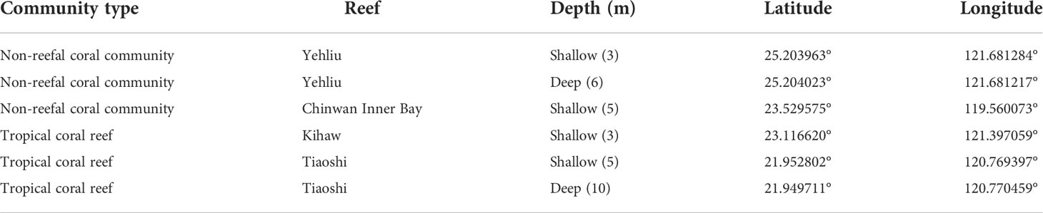
Table 1 The community type, depth and the GPS coordinates of the six survey sites on four reefs.
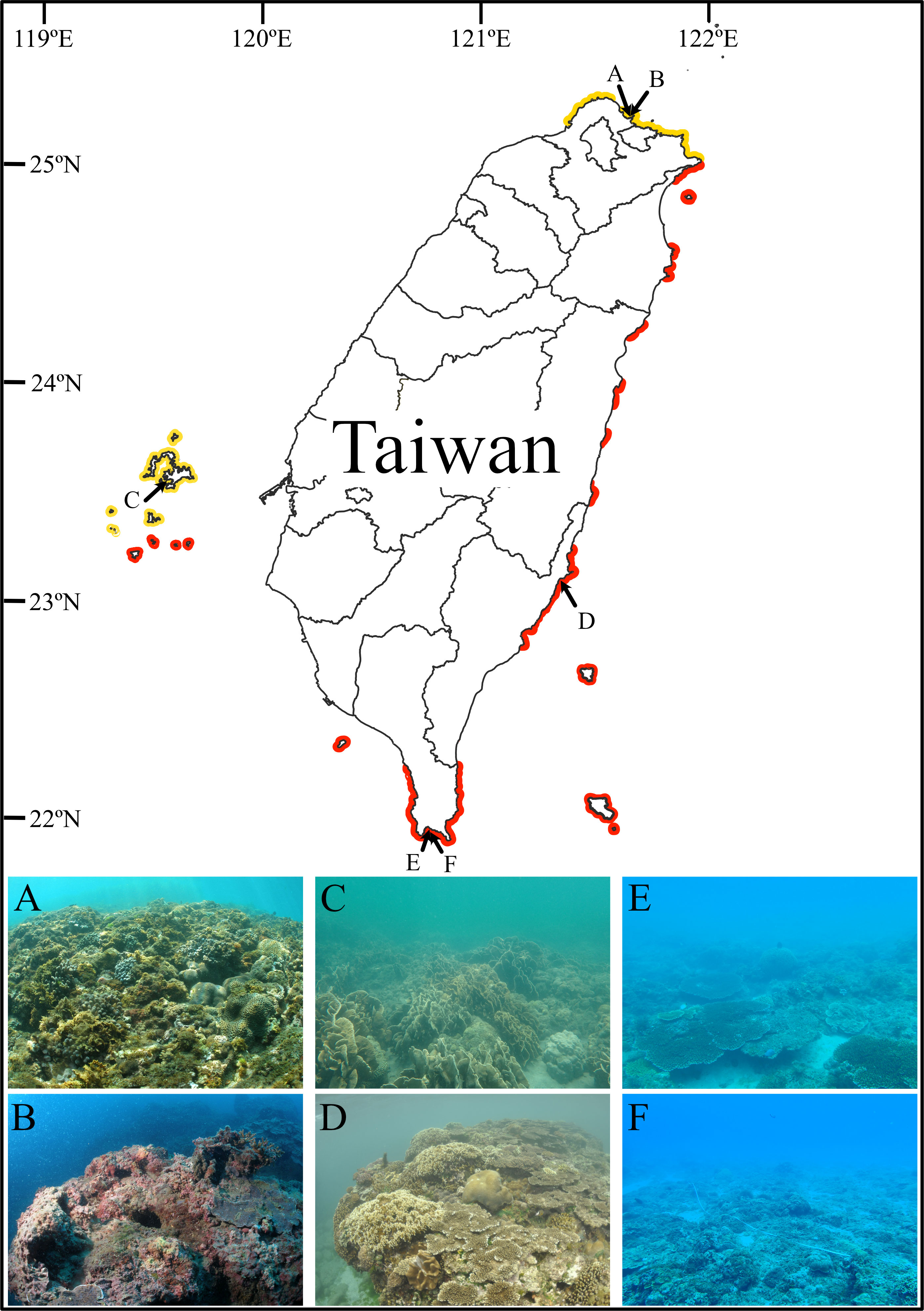
Figure 1 Locations of the six survey sites at four reefs in Taiwan. The six sites include the shallow (A) and deep sites (B) in Yehliu, the shallow sites in Chinwan Inner Bay (C) and Kihaw (D), and the shallow (E) and deep sites (F) in Tiaoshi. The red and yellow lines indicate the distribution range of tropical coral reefs (in red) and non-reefal coral communities (in yellow) in Taiwan. The distribution map was modified from Dai (2018); Keshavmurthy et al. (2019), and Kuo et al. (2022a).
2.2 Field survey methods
Three transects were placed consecutively, a few meters apart from each other, along depth contours parallel to the shoreline at each site. Alternatively, three transects were deployed in parallel for short reefs. The standard transect length used in this study was 15 m due to underwater topographic limitations and the availability of suitable habitats for corals—continuous hard substrates. However, one transect at the shallow site (5m) of Tiaoshi was 14 m long because of operator error. A total of 18 transects (j = 18) at six sites were surveyed for this study between April and July in 2019.
We adopted the concept of the Chain Intercept Transect method to lay out transects according to reef contouring (Porter, 1972; Hughes and Jackson, 1985; English et al., 1997; Hill and Wilkinson, 2004). The benthic community of each transect was recorded by survey divers using Olympus TG-4 camera with a waterproof housing and a video light fixed at the height of ca. 20 cm above substrates. Recording speed was maintained at two meters per minute to ensure a stable and clear visualization of substrates and transect line scales. To minimize the observer bias and to ensure quality and consistency, the identification of the benthic community was conducted by the same most experienced researcher.
2.3 Benthic community identification and data processing
We identified hard corals (HC), including the scleractinians, Heliopora and Millepora, to species level. The rest of the benthos and substrates were identified as soft coral (SC), recently killed coral (RKC), nutrient indicator algae (NIA), turf algae (TF), crustose coralline algae (CCA), sponge (SP), rock (RC), rubble (RB), sand (SD), silt/clay (SI), and other substrates (OT). The data is available at https://doi.org/10.5061/dryad.0rxwdbs35.
The quantification of each category on each transect was first calculated using the LIT method. Briefly, the substrate type at each sampling point with one cm interval was assigned to one of the twelve categories. The percentage cover of each category on each transect was calculated by dividing the cumulative lengths of the category by the total length of the transect (1400 cm or 1500 cm). To further evaluate the compositions of hard and soft corals along each transect, colony number, average colony size, and species richness of both were calculated. Species evenness and diversity of hard corals were determined by Pielou evenness (J) and Shannon-Wiener index (H’), respectively. Herein, we term “LIT datasets” and “LIT communities” to represent the data and communities obtained by the LIT method. LIT datasets and LIT communities were used as baselines for comparison with the PIT method.
To reduce the variability caused by observers or transect placement when comparing the two sampling methods, we did not lay out transects explicitly for the PIT method in the field. Instead, the datasets of the PIT method were extracted from our empirical LIT datasets. The datasets and communities generated using the PIT method are herein referred to as “PIT datasets” and “PIT communities.”
2.4 Data analysis
2.4.1 The optimum sampling interval for the Point Intercept Transect method
The optimum sampling interval for the PIT method is defined as the minimum number of random sampling points required to generate a PIT community comparable to the coral cover estimated by the LIT method of the same transect. All else being equal, if the number of sampling points used is less than the minimum required, the coral cover among PIT communities generated from the same number of random sampling points results in considerable variation, which implies an unreliable estimate of coral cover. In contrast, an excessive number of sampling points (overly more than the minimum number of sampling points required) may not substantially improve the accuracy of coral cover estimates and thus be a waste of sampling effort, as described in Bros and Cowell (1987).
We first used the bootstrap method (Efron, 1979; Manly, 1992) with Monte Carlo approach to resample PIT communities from LIT datasets. The bootstrap approach is one of the resampling techniques which has been applied in a wide range of ecological research, from individual species to community-level (summarized by Manly, 2007). One of its applications is to evaluate the sampling sufficiency for sampling design by calculating the confidence interval of the data generated from the limited empirical data (Bros and Cowell, 1987; Manly, 1992; Pillar, 1998). In this study, this produced surrogate samples which serve as proxies for PIT samples that were obtained empirically. The resampling procedure is described as follows (Figure 2):
(i) x sampling point was selected without replacement from one of the 18 LIT datasets to form a PIT community. For instance, one sampling point (x = 1) was randomly selected from transect j1 to form a PIT community with one sampling point. Then the selected sampling point(s) was restored to the original LIT dataset before the next resampling. This process was repeated for additional 199 times to form a total of 200 PIT communities (n = 200) with one sampling point (x = 1);
(ii) calculate the percentage cover of each benthic category for each of the n PIT communities;
(iii) repeat procedures (i) and (ii) by selecting x sampling points to calculate the SD of the TCC of each set of n PIT communities with the same number of x points. x is equal to 2, 3, 4,…, i-2, i-1, and i. In total, i x n PIT communities were generated. i is the number of all sampling points of a given transect (i = 1,400 and 1,500 for 14 m and 15 m transect, respectively). When x = i, the PIT benthic community composition is equal to the LIT benthic community along the same transect, and
(iv) apply procedures (i), (ii), and (iii) on all the remaining 17 LIT datasets. There were i × n × j PIT communities generated.
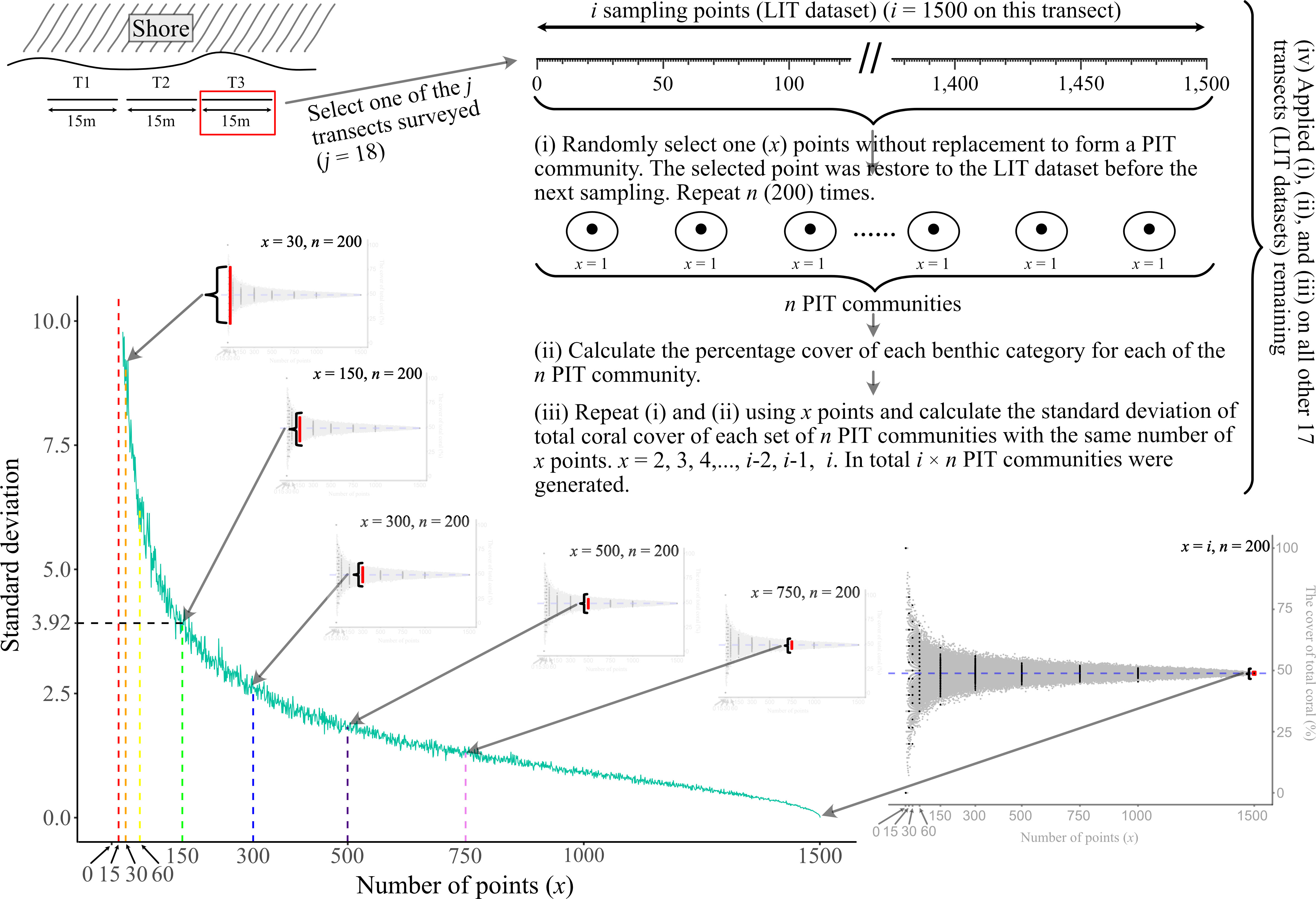
Figure 2 The visual guide of the resampling procedure using the bootstrap method with Monte Carlo approach. LIT and PIT are the abbreviation of Line Intercept Transect and Point Intercept Transect.
Second, scatter plots were used to illustrate the TCC, of the PIT community generated by different sampling points at each LIT transect (Bros and Cowell, 1987). Accumulation curves were used to illustrate the relationship between the number of sampling points and the accuracy, in which the latter was represented by the SD of the TCC of the 200 PIT communities with the same number of sampling points (x) on each transect (Figure 2). Two hundred times of bootstrap sampling is sufficient as the accumulation curves of 200, 500, and 1000 times of bootstrap sampling were similar (Supplementary Figure 1). Lower SD indicates that the TCC of PIT communities is closer to that of LIT communities, which implies a lesser difference between the two methods. However, as the accumulation curve was fairly smooth without an explicit elbow point, we used the SD of 3.92 (95% confidence limit) as a reference criteria to obtain the optimum sampling interval (minimum number of sampling points required) of PIT (Bros and Cowell, 1987). Based on the criteria, the range of the number of sampling points with SD <3.92 would fall within the range of accuracy (i.e., the TCC of the PIT method is within the 95% confidence interval of the TCC of the LIT method on the same transect). Those number of points, which are evenly distributed on a transect, would be determined as the optimum sampling interval for the PIT method. In addition, to examine if the optimum sampling interval is influenced by the types of coral community, we compared the optimum sampling intervals for the PIT method between tropical coral reefs and non-reefal coral communities using Mann-Whitney U tests.
Third, other than estimating the optimal sampling interval at the population level using TCC as the index, we also want to estimate it at the community level, considering other sessile organisms such as turf algae, macroalgae, and sponges compete for limited space with corals. For this statistic, we merged the 12 categories identified into the ten categories of Reef Check’s Tropical Program protocol (Hodgson et al., 2006). We then used multivariable indices (i.e., dissimilarity matrix indices) to estimate the optimum sampling interval at the community level. The compositions of the benthic community generated by the PIT method using the optimum sampling interval should be similar to those by LIT. The Bray-Curtis dissimilarity index (Bray and Curtis, 1957) of individual community composition between each PIT community and LIT community of the same transect was first calculated. Accumulation curves were then used to determine the relationship between the sampling intervals and the average Bray-Curtis dissimilarity index for each of the 200 PIT communities with the same number of random points. This summary statistic used six different numbers of random sampling points (15, 30, 60, 150, 300, and 750) evenly distributed on a 15 m transect instead of continuous increments. These six numbers of random sampling points were selected to represent the several commonly used sampling intervals in the coral reef benthic survey; i.e., 50 cm (30 random points), 25 cm (60 random points), and 10 cm (150 random points), with additional very-fine scales – 2 cm (750 random points) and 5 cm (300 random points), and very-large-scale – 100 cm (15 random points), to explore the accuracy across a wide range of intervals. Intervals are cited herein as PIT 100, PIT 50, PIT 25, PIT 10, PIT 5, and PIT 2. The resampling procedure and statistical analyses were performed in R v. 4.0.3 (R Core Team, 2020) using the “vegan” package (Oksanen et al., 2020). The R codes of the resampling procedure are provided in the Supplementary Material.
2.4.2 Testing the dependency between optimum sampling interval and transect length
The procedure to test if the optimum sampling interval depends on transect length is described as follows (Supplementary Figure 2):
(v) the three transects laid out at each site were attached end-to-end to form a 45-m (except for one 44 m) long virtual transect. The three transects were combined from the same site to reduce the random site effect. A total of six long virtual transects were constructed for the six surveyed sites;
(vi) five repeated, k meters long each, subset transects were randomly extracted from each of the six 45 m virtual transects. A subset transect was formed by selecting continuous sampling points with 1 cm interval from a random starting point. Continuous sampling, instead of interval sampling, was used to maintain the spatial structure of the benthic community. For instance, a 10 m subset transect was extracted by randomly selecting 1000 continuous sampling points along the 45 m virtual transect with 4500 sampling points. A total of 30 subset transects were generated (five transects from each site). Each subset transect served as the LIT dataset with i sampling points (i = 100k);
(vii) apply procedures (i), (ii), and (iii) on the thirty k-meters subset transects generated from the procedure (vi) to calculate the percentage cover of each benthic category of each of the n PIT communities; and
(viii) repeat procedures (vi) and (vii) with k = 10, 20, 30, and 40, respectively.
The two analyses that applied to the 15-m transects described earlier, including (1) accumulation curves of the SD of the TCC of each of the 200 PIT communities generated from the same number of random points on each transect and (2) accumulation curves of the six intervals of interest (PIT 2, PIT 5, PIT 10, PIT 25, PIT 50 and PIT 100) and the average Bray-Curtis dissimilarity index of each set of 200 PIT communities with the same number of random points, were used to determine the optimum sampling intervals for the transect lengths of interest. The actual numbers of random sampling points used for each transect length are provided in Supplementary Table 2. The R codes for attaching transects end-to-end and the resampling procedure is provided in the Supplementary Material.
2.4.3 The accuracy of total coral cover estimated by the Point Intercept Transect method compared to the Line Intercept Transect method
To evaluate the performance of each potential optimum interval, we tested those intervals on the empirical dataset. The TCC was calculated from each of the 18 LIT datasets using the PIT method with 100, 50, 25, 10, 5, and 2 cm sampling intervals. Root mean square error (RMSE) was computed and defined as the deviation from the TCC estimated from 18 PIT communities with the same interval to the perfect fit line (i.e., a 1:1 relationship between observed and predicted values). The elbow of the plotted RMSE curve was identified as the minimum interval required.
3 Results
3.1 Benthic community composition on empirical transects
The total coral (hard and soft), rock, and nutrient indicator algae were the top three major benthic components of the 18 LIT communities surveyed. The average coverages (± SD) were 35.69 ± 3.62%, 27.17 ± 4.13%, and 21.01 ± 6.02%, respectively (Figure 3 and Supplementary Table 3). The average coverages of sand and silt/clay were 7.40 ± 2.55% and 4.80 ± 2.31%, respectively, while the rest components, including recently killed corals, sponges, rubbles, and others, covered less than 5% of the substrates (Supplementary Table 3).
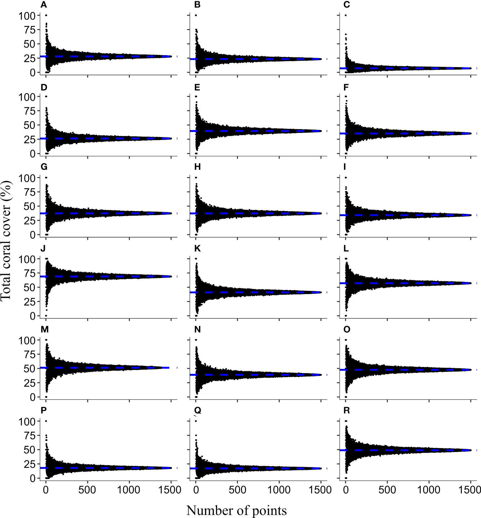
Figure 3 The bell-shaped distribution of the total coral cover (TCC) in relation to the number of random sampling points generated by bootstrap sampling on 18 LIT datasets. The eighteen communities were in the shallow (A-C) and deep sites (D-F) in Yehliu, the shallow sites in Chinwan Inner Bay (G-I) and Kihaw (J-L), and the shallow (M–O) and deep sites (P-R) in Tiaoshi. The order of transects within each habitat is synchronized with the order in Supplementary Table 3. The horizontal blue dashed line indicates the TCC of each transect measured with the LIT method.
The TCC on each transect ranged between 7.06% and 68.76% (Figures 3C, J and Supplementary Table 3). The average colony number, colony size, species richness, and Pielou evenness (J) per transect were 37.53 ± 3.38 colonies, 14.36 ± 0.66 cm, 15.00 ± 1.67 species, and 0.30 ± 0.02, respectively (Supplementary Table 3). The highest TCC, the first transect in Kihaw, was contributed by 63 colonies (18 species) with an average colony size and evenness of 16.38 cm and 0.28, respectively (Supplementary Table 3). In contrast, the third transect at the shallow site in Yehliu featured the lowest TCC, species richness (5 species), and coral colony abundance (7 colonies); however, coral colonies here in average are larger (15.14 cm) and species evenness is high (0.42) (Supplementary Table 3). The coral assemblage on the second transect at the Tiaoshi deep site (TCC = 16.99%) was featured with the largest (19.62 cm) average colony size, contributed by 13 colonies (11 species) (Supplementary Table 3). The smallest (9.24 cm) average colony size was recorded on another transect (the first) of the same site. In addition, the similar TCC (17.85%) was contributed by 29 colonies (19 species), which is two-fold more than that of the previous transect (Supplementary Table 3).
3.2 The optimum sampling interval for the Point Intercept Transect method
The TCC of each PIT community formed a horizontal, bell-shaped distribution, with peak values corresponding to the TCC of their related LIT community (Figure 3). The distribution was most symmetrical when the TCC of the LIT community was around 50% (e.g., Figure 3M). It was positively skewed when TCC was higher than 50% (e.g., Figure 3J) and was negatively skewed, when TCC was lower than 50% (e.g., Figure 3C). The TCC of PIT communities varied, ranging from 0% to 100% when low numbers of random sampling points were selected. With an increase in the number of random sampling points, the TCC of the PIT community started to converge significantly toward the same level as the TCC of the LIT community on the same transect (Figure 3).
The SD of the TCC for each set of the 200 PIT communities with different random sampling points decreased rapidly with the increasing number of random sampling points (Figure 4A and Supplementary Figure 3). The accumulation curves of the 18 transects surveyed were similar except for one transect with the lowest TCC of 7.06% (transect three at the shallow depth of Yehliu, see Supplementary Table 3), where its SD decreased faster than the rest of the transects (Figure 4A and Supplementary Figure 3). The average (and maximum) SD of the 18 transects was 45.58 (50.12), with one random sampling point selected. The SD declined to 11.62 (13.56), 8.29 (9.18), 5.80 (6.77), 3.54 (4.08), 2.33 (2.77), and 1.16 (1.32) when random sampling point numbers selected were 15 (PIT 100), 30 (PIT 50), 60 (PIT 25), 150 (PIT 10), 300 (PIT 5), and 750 (PIT 2), respectively (Figure 4A and Table 2). Of the 18 transects, 14 transects fell within the range of accuracy, i.e., with SD <3.92, when using 150 random sampling points (PIT 10), while three and one transects fell within the range of accuracy when using 300 (PIT 5) and 60 sampling points (PIT 25). All 18 transects showed SD values outside of the range of accuracy for PIT 2, PIT 50, and PIT 100. Therefore, overall, PIT 10 was determined as the optimum sampling interval for PIT (Supplementary Table 4). Meanwhile, there was no significant difference in the optimum sampling interval recommended between the tropical coral reefs and the non-reefal coral communities (Mann–Whitney Test, p = 0.36).
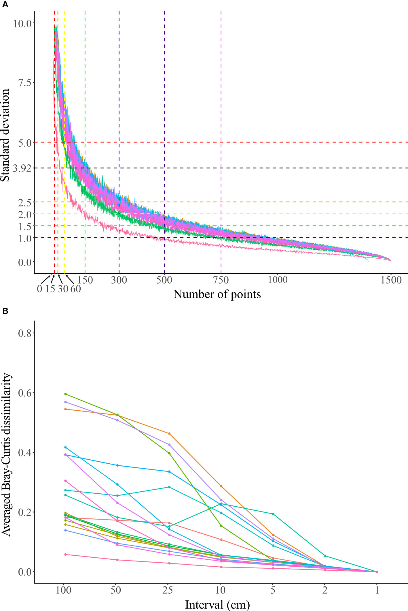
Figure 4 (A) The standard deviation (SD) of the TCC of each set of 200 PIT communities with different randomly sampling points from 15 m transects. The horizontal dashed lines mark SDs of 5 (red), 3.92 (black), 2.5 (orange), 2 (yellow), 1.5 (green), and 1 (blue), and the vertical dashed lines mark the number of points using PIT 100 (15 points, red), PIT 50 (30 points, orange), PIT 25 (60 points, yellow), PIT 10 (150 points, green), PIT 5 (300 points, blue), PIT 3 (500 points, indigo), and PIT 2 (750 points, purple). (B) The Bray-Curtis dissimilarity index between the PIT community and the LIT community on the same transect. Each dot represents the average of 200 PIT communities with the same interval. The color of the accumulation curves represent the 18 transects surveyed and are referred to in Supplementary Figure 3.
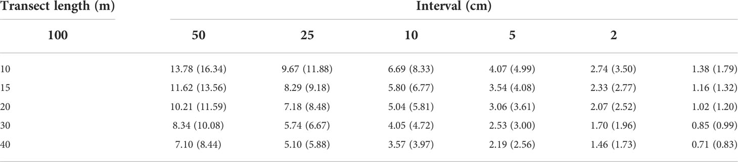
Table 2 The average (maximum) standard deviation of the total coral cover of 200 PIT communities using six different sampling intervals (PIT 100, PIT 50, PIT 25, PIT 10, PIT 5, and PIT 2) for different lengths of transect.
In terms of dissimilarity of community compositions, there was a decreasing trend with decreasing sampling intervals between the LIT and PIT communities (Figure 4B). The differences in the average dissimilarity between LIT and PIT communities varied among transects, ranging between 0.06 and 0.60, with an average of 0.29 at PIT 100. The average (and highest) dissimilarity values of the 18 transects were reduced to 0.23 (0.53), 0.17 (0.46), 0.11 (0.29), 0.06 (0.19), and 0.02 (0.05) at PIT 50, PIT 25, PIT 10, PIT 5, and PIT 2, respectively (Figure 4B and Supplementary Table 5). From the accumulation curves, three elbow points were detected among the 18 transects, with the majority (11 out of 18 transects) at 10 cm intervals (PIT 10), while only two and five transects at 5 cm intervals (PIT 5) and 2 cm intervals (PIT 2), respectively (Figure 4B and Supplementary Table 5).
3.3 Testing the dependency between optimum sampling interval and transect length
The average SD of individual 200 PIT communities at the same interval among the 30 equal-length subset transects decreased with increasing transect length (Figures 5A, C, E, G, and Table 2). The PIT interval where the average SD fell within the range of accuracy (SD <3.92) were PIT 5 for 10-m transects, PIT 10 for 20-m and 30-m transects, and PIT 25 for the 40-m transect (Table 2). More strictly, by only accounting for the maximum SD <3.92, the optimum sampling intervals were PIT 5 for 10-m transects and PIT 10 for 20-m, 30-m, and 40-m transects (Figures 5A, C, E, G, and Table 2). As shown on the accumulation curves of the average Bray-Curtis dissimilarity index, the elbow points were detected between PIT 10 and PIT 2, regardless of transect length (Figures 5B, D, F, H).
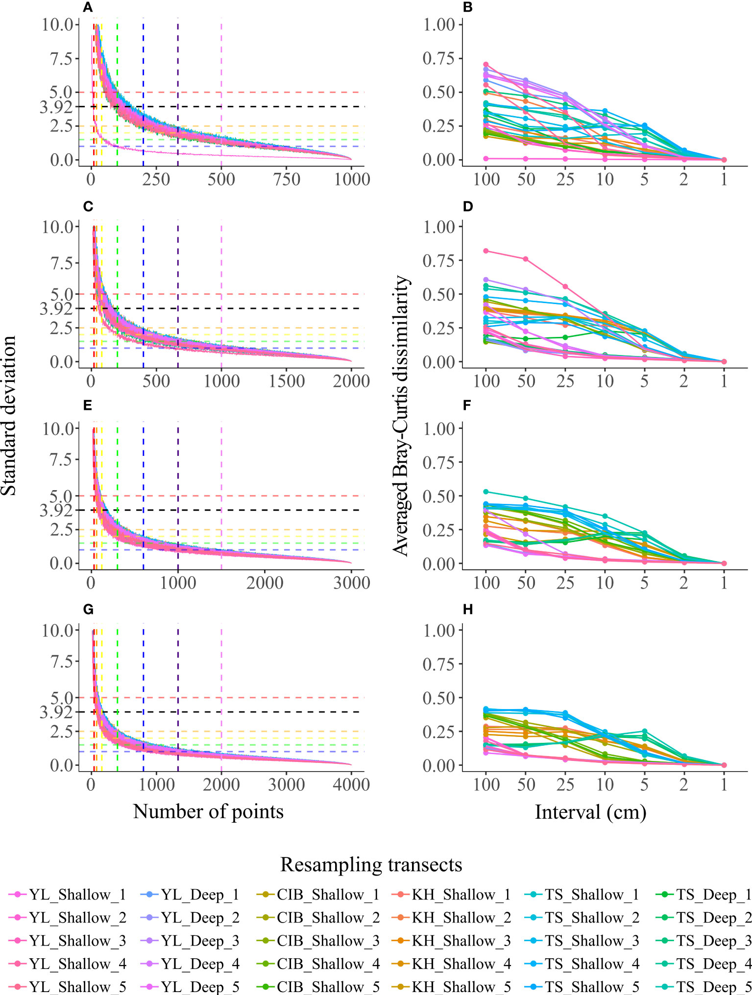
Figure 5 The accumulation curves of the standard deviation (SD) of the TCC of each set of 200 PIT communities with different randomly sampled points (A, C, E, G), and the average of the 200 Bray-Curtis dissimilarity indexes between each PIT community at the same interval and LIT community (B, D, F, H) on different transect lengths. The transect lengths were 10 m (A, B), 20 m (C, D), 30 m (E, F), and 40 m (G, H). The horizontal dashed lines in A, C, E, G mark SDs of 5 (red), 3.92 (black), 2.5 (orange), 2 (yellow), 1.5 (green), and 1 (blue), and the vertical dashed lines mark the points used in PIT 100 (red), PIT 50 (orange), PIT25 (yellow), PIT 10 (green), PIT 5 (blue), PIT 3 (indigo), and PIT 2 (purple).
3.4 Total coral cover error estimated by the Point Intercept Transect method compared to the Line Intercept Transect method
The TCC measured by the PIT method was closer to those by the LIT method at finer sampling intervals (Figure 6A). The RMSE curve showed a decreasing trend with decreasing sampling intervals, with the elbow identified at the 10 cm sampling interval (PIT 10) (Figure 6B).
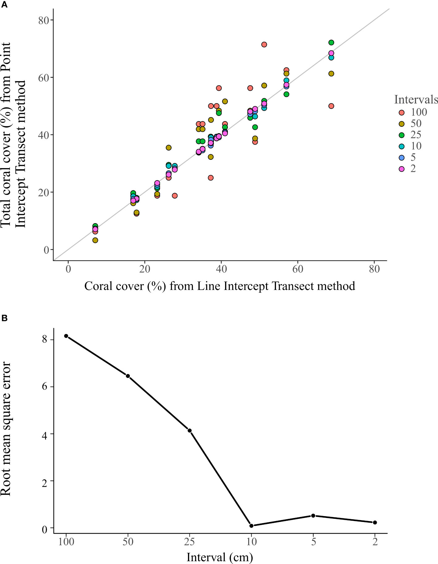
Figure 6 The total coral cover (TCC) of PIT communities generated from the 18 LIT communities survey over different sampling intervals. Each dot represents one PIT community, and colors indicate different intervals (A). The root mean square error of the TCC measured using the PIT method to the TCC measured using the LIT method on each of the 18 transects at different sampling intervals (B).
4 Discussion
Our analysis revealed that current sampling intervals of the PIT method used in the literature could not accurately estimate the status of the benthic community, specifically the TCC, and act as an alternative to replace the LIT method. Instead, the range between 2 cm (PIT 2) and 10 cm (PIT 10) were better options, depending on the transect length and statistics parameters used (Table 2).
A 10 cm interval (PIT 10) is the recommended sampling interval in most of our study combinations of point interval and transect length. It is between the recommended 4 cm and 25 cm intervals in two other studies conducted in Brazil and Réunion Island (Segal and Castro, 2001; Facon et al., 2016). The variation between those studies and our study might be attributed to the taxonomic resolution, statistical methods used, and the reef environment of each study area. Segal and Castro (2001) sought an interval for measuring the cover of individual species rather than TCC. Finer operational taxonomic units (OTUs) require shorter intervals. For instance, PIT 25 is sufficient for identifying the ten OTUs used by the Tropical Program of Reef Check while PIT 10 is necessary for identifying over 30 OTUs, including identifying corals to the genus level, as reported in the study conducted at Réunion Island (Facon et al., 2016).
The statistical methods also play a role in determining the optimum sampling interval. Both our study and that of Facon et al. (2016) discriminate the optimal sampling interval by identifying the elbow on the accumulation curves of the dissimilarity between PIT and LIT communities with ten OTUs. Yet, our result (PIT 2) was more conservative when using the Bray-Curtis dissimilarity index than the result (PIT 25) of Facon et al. (2016), which used Pearson correlation coefficients (Legendre and Legendre, 1998).
The variation in the status of benthic communities also alters the optimum sampling interval. Theoretically, TCC, coral colony abundance, colony size distribution, and pattern of colonies distributed along the transect would affect how quickly reaching an optimum interval in the PIT method. In our study, it requires the highest number of sampling points to achieve the optimum interval on the transect with 50% of TCC. The number was reduced along with either a decrease or an increase in TCC (Supplementary Table 4). While our study was conducted on reefs across well-developed tropical coral reefs and non-reefal coral communities, Segal and Castro (2001) and Facon et al. (2016)’s work were conducted on the less-developed reefs in the Abrolhos Archipelago, Brazil, and the Indian Ocean reefs on Réunion Island, respectively. It is hard to distinguish what causes the difference in the recommended optimum sampling intervals without the knowledge of the reef status. This highlights the need to further research on how the distribution patterns of the benthic community affect the accuracy of survey methods.
Our study showed that there was no significant difference in optimum intervals between the tropical coral reefs and non-reefal coral communities. The influence of habitat structure on benthic community composition was more significant with an increase in transect length (Figures 4B, 5B, D, F, H). The lack of a similar pattern among transects in the same type of reef indicates that the complexity of the benthic community within sites is more apparent than among reefs. This also suggests that the historical environmental conditions have significantly changed recently due to increasing natural disturbances and human-induced stresses at larger and local scales (Ribas-Deulofeu et al., 2016). Local stressors cause declines in reef conditions, reduce resilience, and postpone recovery from natural disturbances (Carilli et al., 2009; Ortiz et al., 2018). Under the stress of climate change-induced extreme disturbances, such as more frequent and severe bleaching events (Hughes et al., 2018), typhoons (Tsuboki et al., 2015; Knutson et al., 2020), and the lack of the ability to recover between disturbances will prevent the full recovery of coral reefs and result in further degradation.
Previous coral reef monitoring studies using PIT 50 on non-permanent transects have reported high annual variations in TCC at the same survey sites without major disturbances between survey censuses (Dai et al., 2004; TEIA, 2016; TEIA, 2017). Our finding that the 50 cm sampling interval (PIT 50) estimates a high variation of TCC might explain the high temporal changes in those studies, as well as emphasize the necessity of using non-permanent transects. Using non-permanent transects for long-term monitoring reduces the effort to set up and maintain the markers and the time consumed in searching for transect markers. This method benefits most when surveyors are familiar with the reef and the benthic community composition is homogeneous within the target survey area. However, several issues need to be considered. First, human errors, such as misidentifying the starting point and direction of transects, are unavoidable. The issue is more profound on less-developed or patchily distributed coral communities. Even a slight displacement of starting point or direction would result in a significantly different community composition. Second, success in consistently relocating the survey spot is highly reliant on the participation of a few experienced key members. It means the project is exposed to the risk of inconsistency in data collection over the long term. Extra care is necessary for interpreting monitoring results.
Applying the permanent transect method requires extra work on marker maintenance; however, it can benefit monitoring programs. It improves the quality of data because it is more consistent, repeatable, and reliable. The results are comparable across survey censuses, and the changes in benthic communities can be more confidently attributed to environmental changes rather than the errors in the sampling method (summary in Hill and Wilkinson, 2004). In addition, permanent transects set up in the field can be used for a variety of projects from citizen science programs to long-term ecological monitoring projects and fine-scale research such as a demographic approach to understand the dynamics of scleractinians in the reef (Edmunds and Riegl, 2020), which enables the enhancement of the quality of citizen science education and helps improve the management strategies.
A comprehensive understanding of the status of coral reef benthic communities requires cooperation between both coral reef scientists and citizen scientists to conduct the survey with consistent and comparable methods. Our results suggest that a 10 cm sampling interval is the minimum necessary when using the PIT method as an alternative to the LIT method. In addition, our results highlight the need for setting up permanent transects for long-term monitoring purposes, as suggested by Reef Check (Hodgson et al., 2006) and GCRMN (Hill and Wilkinson, 2004), to improve the consistency, repeatability, and reliability of data collection (Hill and Wilkinson, 2004).
Data availability statement
The datasets presented in this study can be found in online repositories. The names of the repository/repositories and accession number(s) can be found below: Kuo et al. (2022b), Data from: Fine intervals are required when using point intercept transects to assess coral reef status, Dryad, Dataset, https://doi.org/10.5061/dryad.0rxwdbs35.
Author contributions
C-YK, C-HT, HH, and CC conceived the study. C-YK, A-TH, Y-YH, and CC conducted the field survey. CC conducted benthic community component identifications. C-YK and A-TH conducted data wrangling. C-YK and C-HT conceived and performed the statistics. C-YK, Y-YH, and WH wrote the first draft of the manuscript. All authors have read and approved the submitted version.
Funding
This study was funded by the Ocean Conservation Administration, Ocean Affairs Council, Taiwan (grant no. 108-C-9), and Biodiversity Research Center, Academia Sinica.
Acknowledgments
Many thanks to Ai-Chi Chung and Meng-Yun Hsieh for helping in conducting the fieldwork and the lab members of the Coral Reef Evolutionary and Ecological Genetic Laboratory of the Biodiversity Research Center, Academia Sinica, Taiwan, and the Penghu Marine Biology Research Center, Fisheries Research Institute, Council of Agriculture, Taiwan, for providing logistical support. We would like to thank Buford C. Pruitt, Jr. for English editing and Dr. Chun-Lin Lee for the comments on the visual guide of resampling procedures. We appreciate the reviewers and editors who assisted in improving this manuscript.
Conflict of interest
The authors declare that the research was conducted in the absence of any commercial or financial relationships that could be construed as a potential conflict of interest.
Publisher’s note
All claims expressed in this article are solely those of the authors and do not necessarily represent those of their affiliated organizations, or those of the publisher, the editors and the reviewers. Any product that may be evaluated in this article, or claim that may be made by its manufacturer, is not guaranteed or endorsed by the publisher.
Supplementary material
The Supplementary Material for this article can be found online at: https://www.frontiersin.org/articles/10.3389/fmars.2022.795512/full#supplementary-material
Supplementary Figure 1 | The accumulation curves of the standard deviation of the TCC of each set of 200 (A), 500 (B), and 1000 (C) PIT communities by the bootstrap method with different randomly sampled points.
Supplementary Figure 2 | The visual guide of the resampling procedure to testing if the optimum sampling interval depends on transect length.
Supplementary Figure 3 | The standard deviation (SD) of the TCC of each set of 200 PIT communities having different randomly sampled points used on each 15 m transect surveyed. Horizontal dashed lines mark SDs of 5 (red), 3.92 (black), 2.5 (orange), 2 (yellow), 1.5 (green), and 1 (blue), and the vertical dashed lines mark the number of points for PIT 100 (15 points, red), PIT 50 (30 points, orange), PIT 25 (60 points, yellow), PIT 10 (150 points, green), PIT 5 (300 points, blue), PIT 3 (500 points, indigo), and PIT 2 (750 points, purple). The color of the accumulation curves represents the 18 transects surveyed.
References
Adjeroud M., Augustin D., Galzin R., Salvat B. (2002). Natural disturbances and interannual variability of coral reef communities on the outer slope of Tiahura (Moorea, French Polynesia): 1991 to 1997. Mar. Ecol. Prog. Ser. 237, 121–131. doi: 10.3354/meps237121
Adjeroud M., Michonneau F., Edmunds P. J., Chancerelle Y., Loma T. L., Penin L., et al. (2009). Recurrent disturbances, recovery trajectories, and resilience of coral assemblages on a South Central Pacific reef. Coral Reefs 28, 775–780. doi: 10.1007/s00338-009-0515-7
Beenaerts N., Berghe E. V. (2005). Comparative study of three transect methods to assess coral cover, richness and diversity. West Ind. Oc. J. Mar. Sci. 4, 29–38. doi: 10.4314/wiojms.v4i1.28471
Beijbom O., Edmunds P. J., Roelfsema C., Smith J., Kline D. I., Neal B. P., et al. (2015). Towards automated annotation of benthic survey images: Variability of human experts and operational modes of automation. PLoS One 10, e0130312. doi: 10.1371/journal.pone.0130312
Bray J. R., Curtis J. T. (1957). An ordination of the upland forest communities of southern Wisconsin. Ecol. Monogr. 27, 325–349. doi: 10.2307/1942268
Bros W. E., Cowell B. C. (1987). A technique for optimizing sample size (replication). J. Exp. Mar. Biol. Ecol. 114, 63–71. doi: 10.1016/0022-0981(87)90140-7
Bryson M., Ferrari R., Figueira W., Pizarro O., Madin J., Williams S., et al. (2017). Characterization of measurement errors using structure-from-motion and photogrammetry to measure marine habitat structural complexity. Ecol. Evol. 7, 5669–5681. doi: 10.1002/ece3.3127
Burns J. H. R., Delparte D., Gates R. D., Takabayashi M. (2015). Integrating structure-from-motion photogrammetry with geospatial software as a novel technique for quantifying 3D ecological characteristics of coral reefs. PeerJ 3, e1077. doi: 10.7717/peerj.1077
Carilli J. E., Norris R. D., Black B. A., Walsh S. M., McField M. (2009). Local stressors reduce coral resilience to bleaching. PLoS One 4, e6324. doi: 10.1371/journal.pone.0006324
Dai C.-F. (2018). “Chapter 7. coastal and shallower water ecosystem,” in Regional Oceanography of Taiwan version II, ed. Jan S. (Taipei, Taiwan: National Taiwan University Press), 263–299.
Dai C.-F., Soong K., Jeng M.-S., Chen C. A., Fan T.-Y. (2004). The Status of Coral Reefs in Taiwan (Taipei, Taiwan: Council of Agriculture, Executive Yuan).
Dodge R. E., Logan A., Antonius A. (1982). Quantitative reef assessment studies in Bermuda: a comparison of methods and preliminary results. Bull. Mar. Sci. 32, 745–760.
Edmunds P., Riegl B. (2020). Urgent need for coral demography in a world where corals are disappearing. Mar. Ecol. Prog. Ser. 635, 233–242. doi: 10.3354/meps13205
Efron B. (1979). Bootstrap methods: another look at jackknife. Ann. Stat. 7, 1–26. doi: 10.1214/aos/1176344552
English S. A., Wilkinson C., Baker V. (1997). Survey Manual for Tropical Marine Resources, 2nd Edn (Townsville, Australia, Australian Institute of Marine Science).
Facon M., Pinault M., Obura D., Pioch S., Pothin K., Bigot L., et al. (2016). A comparative study of the accuracy and effectiveness of line and point intercept transect methods for coral reef monitoring in the southwestern Indian ocean islands. Ecol. Indic. 60, 1045–1055. doi: 10.1016/j.ecolind.2015.09.005
Francini-Filho R. B., Coni E. O. C., Meirelles P. M., Amado-Filho G. M., Thompson F. L., Pereira-Filho G. H., et al. (2013). Dynamics of coral reef benthic assemblages of the Abrolhos Bank, Eastern Brazil: inferences on natural and anthropogenic drivers. PLoS One 8, e54260. doi: 10.1371/journal.pone.0054260
Graham N. A. J., Chong-Seng K. M., Huchery C., Januchowski-Hartley F. A., Nash K. L. (2014). Coral reef community composition in the context of disturbance history on the Great Barrier Reef, Australia. PLoS One 9, e101204. doi: 10.1371/journal.pone.0101204
Hargreaves-Allen V. A., Mourato S., Milner-Gulland E. J. (2017). Drivers of coral reef marine protected area performance. PLoS One 12, e0179394. doi: 10.1371/journal.pone.0179394
Harris A., Sheppard C. (2008). “Status and recovery of the coral reefs of the Chagos Archipelago, British Indian Ocean Territory,” in CORDIO Status Report 2008, eds. Obura D., Tamelander J., Linden O. (Mombasa: CORDIO: Coastal Oceans Research and Development, Indian Ocean), 61–70.
Hill J., Wilkinson C. (2004). Methods for Ecological Monitoring of Coral Reefs (Townsville, Australia: Australian Institute of Marine Science). Available at: https://www.cbd.int/doc/case-studies/tttc/tttc-00197-en.pdf.
Hodgson G. (1999). A global assessment of human effects on coral reefs. Mar. Pollut. Bull. 38, 345–355. doi: 10.1016/S0025-326X(99)00002-8
Hodgson G., Hill J., Kiene W., Maun L., Mihaly J., Liebeler J., et al. (2006). Reef Check Instruction Manual: A Guide to Reef Check Coral Reef Monitoring (Pacific Palisades, California, USA: Reef Check Foundation).
Hughes T. P. (1996). Demographic approaches to community dynamics: a coral reef example. Ecology 77, 2256–2260. doi: 10.2307/2265718
Hughes T. P., Anderson K. D., Connolly S. R., Heron S. F., Kerry J. T., Lough J. M., et al. (2018). Spatial and temporal patterns of mass bleaching of corals in the Anthropocene. Science 359, 80–83. doi: 10.1126/science.aan8048
Hughes T. P., Jackson J. B. C. (1985). Population dynamics and life histories of foliaceous corals. Ecol. Monogr. 55, 141–166. doi: 10.2307/1942555
Jackson J., Donovan M., Cramer K., Lam V. (2014). Status and Trends of Caribbean Coral Reefs: 1970-2012 (Gland, Switzerland: Global Coral Reef Monitoring Network, IUCN).
Kershaw K. A. (1957). The use of cover and frequency in the detection of pattern in plant communities. Ecology 38, 291–299. doi: 10.2307/1931688
Keshavmurthy S., Kuo C.-Y., Huang Y.-Y., Carballo-Bolaños R., Meng P.-J., Wang J.-T., et al. (2019). Coral reef resilience in Taiwan: lessons from long-term ecological research on the coral reefs of Kenting National Park (Taiwan). J. Mar. Sci. Eng. 7, 388. doi: 10.3390/jmse7110388
Kimura T., Chou L. M., Huang D., Tun K., Goh E. (2022). Status and Trends of East Asian Coral Reefs: 1983–2019 (Global Coral Reef Monitoring Network, East Asia Region).
Knutson T., Camargo S. J., Chan J. C. L., Emanuel K., Ho C.-H., Kossin J., et al. (2020). Tropical cyclones and climate change assessment: part II: projected response to anthropogenic warming. Bull. Am. Meteorol. Soc. 101, E303–E322. doi: 10.1175/BAMS-D-18-0194.1
Kohler K. E., Gill S. M. (2006). Coral point count with Excel extensions (CPCe): a visual basic program for the determination of coral and substrate coverage using random point count methodology. Comput. Geosci. 32, 1259–1269. doi: 10.1016/j.cageo.2005.11.009
Komyakova V., Munday P. L., Jones G. P. (2013). Relative importance of coral cover, habitat complexity and diversity in determining the structure of reef fish communities. PLoS One 8, e83178. doi: 10.1371/journal.pone.0083178
Kuo C.-Y., Keshavmurthy S., Huang Y.-Y., Ho M.-J., Hsieh H. J., Hsiao A.-T., et al. (2022a). “Transitional coral ecosystems of Taiwan in the era of changing climate,” in Coral Reefs of the Eastern Asia under Anthropogenic Impacts, eds. Takeuchi I., Yamashiro H. (Cham, Switzerland: Springer Nature).
Kuo C.-Y., Tsai C.-H., Huang Y.-Y., Heng W. K., Hsiao A.-T., Hsieh H. J., et al. (2022b). Data from: Fine intervals are required when using point intercept transects to assess coral reef status, Dryad, Dataset. doi: 10.5061/dryad.0rxwdbs35
Loya Y. (1972). Community structure and species diversity of hermatypic corals at Eilat, Red Sea. Mar. Biol. 13, 100–123. doi: 10.1007/BF00366561
Loya Y. (1978). “Plotless and transect methods,” in Coral Reefs: Research Methods, eds. Stoddart D. R., Johannnes R. E. (Paris: UNESCO), 197–217.
Loya Y., Slobodkin L. B. (1971). The coral reefs of Eilat (Gulf of Eilat, Red Sea). Symp. Zool. Soc. Lond. 28, 117–139.
Manly B. F. J. (1992). Bootstrapping for determining sample sizes in biological studies. J. Exp. Mar. Biol. Ecol. 158, 189–196. doi: 10.1016/0022-0981(92)90226-Z
Manly B. F. J. (2007). Randomization, Bootstrap and Monte Carlo Methods in Biology, 3rd Edn (New York: Chapman and Hall/CRC).
Nadon M.-O., Stirling G. (2006). Field and simulation analyses of visual methods for sampling coral cover. Coral Reefs 25, 177–185. doi: 10.1007/s00338-005-0074-5
Obura D., Gudka M., Samoilys M., Osuka K., Mbugua J., Keith D. A., et al. (2022). Vulnerability to collapse of coral reef ecosystems in the Western Indian Ocean. Nat. Sustain. 5, 104–113. doi: 10.1038/s41893-021-00817-0
Ohlhorst S. L., Liddell W. D., Taylor R. J., Taylor J. M. (1988). “Evaluation of reef census techniques,” in Proceedings of the 6th International Coral Reef Symposium, Vol. 2, Townsville, QLD, Australia. 319–324.
Oksanen J., Blanchet F. G., Friendly M., Kindt R., Legendre P., McGlinn D., et al. (2020) Vegan: Community Ecology package. version 2.5-7. Available at: https://CRAN.R-project.org/package=vegan.
Ortiz J.-C., Wolff N. H., Anthony K. R. N., Devlin M., Lewis S., Mumby P. J. (2018). Impaired recovery of the Great Barrier Reef under cumulative stress. Sci. Adv. 4, eaar6127. doi: 10.1126/sciadv.aar6127
Pizarro O., Friedman A., Bryson M., Williams S. B., Madin J. (2017). A simple, fast, and repeatable survey method for underwater visual 3D benthic mapping and monitoring. Ecol. Evol. 7, 1770–1782. doi: 10.1002/ece3.2701
Porter J. W. (1972). Patterns of species diversity in Caribbean reef corals. Ecology 53, 745–748. doi: 10.2307/1934796
Pratchett M. S., Trapon M., Berumen M. L., Chong-Seng K. (2011). Recent disturbances augment community shifts in coral assemblages in Moorea, French Polynesia. Coral Reefs 30, 183–193. doi: 10.1007/s00338-010-0678-2
R Core Team (2020). R: A Language and Environment for Statistical Computing (Vienna, Austria: R Foundation for Statistical Computing). Available at: https://www.R-project.org/.
Ribas-Deulofeu L., Denis V., De Palmas S., Kuo C.-Y., Hsieh H. J., Chen C. A. (2016). Structure of benthic communities along the Taiwan latitudinal gradient. PLoS One 11, e0160601. doi: 10.1371/journal.pone.0160601
Russ G. R., Rizzari J. R., Abesamis R. A., Alcala A. C. (2021). Coral cover a stronger driver of reef fish trophic biomass than fishing. Ecol. Appl. 31, e02224. doi: 10.1002/eap.2224
Segal B., Castro C. B. (2001). A proposed method for coral cover assessment: a case study in Abrolhos, Brazil. Bull. Mar. Sci. 69, 487–496.
Selig E. R., Bruno J. F. (2010). A global analysis of the effectiveness of marine protected areas in preventing coral loss. PLoS One 5, e9278. doi: 10.1371/journal.pone.0009278
Souter D., Planes S., Wicquart J., Logan M., Obura D., Staub F. (2020). “Chapter 2. Status of coral reefs of the world,” in Status of Coral Reefs of the World: 2020 (The Global Coral Reef Monitoring Network and the International Coral Reef Initiative). https://gcrmn.net/2020-report/
Stoddart D. R. (1969). Ecology and morphology of recent coral reefs. Biol. Rev. 44, 433–498. doi: 10.1111/j.1469-185X.1969.tb00609.x
Stoddart D. R. (1972). "Field methods in the study of coral reefs," in Proceedings of the first international symposium on corals and coral reefs, Mandapam Camp, India. 71–80.
Strain E. M. A., Edgar G. J., Ceccarelli D., Stuart-Smith R. D., Hosack G. R., Thomson R. J. (2019). A global assessment of the direct and indirect benefits of marine protected areas for coral reef conservation. Divers. Distrib. 25, 9–20. doi: 10.1111/ddi.12838
TEIA (2016). Reef Check Taiwan Annual Survey Report 2016 (Taipei, Taiwan: Taiwan Environmental Information Association). Available at: https://www.slideshare.net/reefcheck/2016-70458046.
TEIA (2017). Reef Check Taiwan Annual Survey Report 2017 (Taipei, Taiwan: Taiwan Environmental Information Association). Available at: https://www.slideshare.net/reefcheck/2017-108449450.
Tsai C.-H., Sweatman H. P. A., Thibaut L. M., Connolly S. R. (2022). Volatility in coral cover erodes niche structure, but not diversity, in reef fish assemblages. Sci. Adv. 8, eabm6858. doi: 10.1126/sciadv.abm6858
Tsuboki K., Yoshioka M. K., Shinoda T., Kato M., Kanada S., Kitoh A. (2015). Future increase of supertyphoon intensity associated with climate change. Geophys. Res. Lett. 42, 646–652. doi: 10.1002/2014GL061793
Wilkinson C. (2000). Status of Coral Reefs of the World: 2000 (Townsville, Australia: Australian Institute of Marine Science). Available at: https://gcrmn.net/resource/status-coral-reefs-world-2000/.
Wilkinson C. (2002). Status of Coral Reefs of the World: 2002 (Townsville, Australia: Australian Institute of Marine Science). Available at: https://gcrmn.net/resource/status-coral-reefs-world-2002/.
Wilkinson C. (2004). Status of Coral Reefs of the World: 2004, Vol. 1 (Townsville, Australia: Australian Institute of Marine Science). Available at: https://gcrmn.net/resource/status-coral-reefs-world-2004-volume-1/.
Wilkinson C. (2008). Status of Coral Reefs of the World: 2008 (Townsville, Australia: Global Coral Reef Monitoring Network and Reef and Rainforest Research Centre). Available at: https://gcrmn.net/resource/status-coral-reefs-world-2008/.
Keywords: benthic community, reef survey methods, LIT, reef check, citizen science, long-term monitoring
Citation: Kuo C-Y, Tsai C-H, Huang Y-Y, Heng WK, Hsiao A-T, Hsieh HJ and Chen CA (2022) Fine intervals are required when using point intercept transects to assess coral reef status. Front. Mar. Sci. 9:795512. doi: 10.3389/fmars.2022.795512
Received: 15 October 2021; Accepted: 08 August 2022;
Published: 27 September 2022.
Edited by:
Nina Yasuda, The University of Tokyo, JapanReviewed by:
Mohammad Reza Shokri, Shahid Beheshti University, Iran;Naoki Kumagai, National Institute for Environmental Studies (NIES), JapanCopyright © 2022 Kuo, Tsai, Huang, Heng, Hsiao, Hsieh and Chen. This is an open-access article distributed under the terms of the Creative Commons Attribution License (CC BY). The use, distribution or reproduction in other forums is permitted, provided the original author(s) and the copyright owner(s) are credited and that the original publication in this journal is cited, in accordance with accepted academic practice. No use, distribution or reproduction is permitted which does not comply with these terms.
*Correspondence: Chaolun Allen Chen, Y2FjQGdhdGUuc2luaWNhLmVkdS50dw==