 Haihang Zhi
 Hui Wu
 Jiaxue Wu
 Wenxia Zhang
 Yihe Wang
- 1State Key Laboratory of Estuarine and Coastal Research, East China Normal University, Shanghai, China, and Southern Marine Science and Engineering Guangdong Laboratory, Zhuhai, China
- 2Southern Marine Science and Engineering Guangdong Laboratory, Zhuhai, China
- 3School of Marine Sciences, East China Normal University, Shanghai, China
The buoyant river plume front exhibits substantial variability in the sea surface under energetic external forcing. Although highly dynamic, the river plume is often “rooted” at specific locations through the bottom river plume front. In this study, we addressed this mechanism using the Pearl River plume as an example based on a well-validated numerical model. With this model, we described the spatiotemporal characteristics of the Pearl River salinity front. It was found that, although the surface Pearl River plume features bimodal extension in summer and winter seasons, owing to the reversal of the seasonal monsoon wind, there is a relatively stable bottom front extending from the river mouth to the downstream region (i.e., in the direction of propagation of Kelvin Wave). The occurrence probability of the bottom front showed that the front location varies only slightly and fixes at ∼8-m isobath. The Empirical Orthogonal Function (EOF) analysis demonstrated that runoff, wind, and tide are major regulating factors. These three factors jointly control the strength and position of the bottom front. In particular, the bottom front moves offshore during the spring tide but onshore during the neap tide, respectively, indicating a different mechanism from the classic frontal trapping theory. The sensitivity experiment without tide indicated that the bottom plume front shrinks significantly, and the river plume becomes more dynamic since it is no longer rooted on the seafloor.
Introduction
The Pearl River is the second largest river in China in terms of freshwater discharge, with an annual-mean runoff of ∼10,000m3/s (Gan et al., 2009). It discharges into the northern South China Sea (NSCS) through eight outlets which are Humen, Jiaomen, Hongqili, Hengmen, Modaomen, Jitimen, Hutiaomen and Yamen (Figure 1). The first four outlets enter a semi-enclosed estuarine bay, namely the Lingdingyang Bay or conventionally the Pearl River Estuary, which receives nearly half of the total upstream runoff (Lai et al., 2015). The Kelvin number of the Pearl River plume in the far-field is about 5 (estimated by the model result of this study), meaning that the plume is large-scale (Garvine, 1995). The average water depth of the Pearl River Estuary is ∼5 m with two deep channels (the West Channel and East Channel) exceeding 10 m. The length of the Pearl River Estuary is ∼60 km from the mouth up to Humen, and the width of its mouth is ∼50 km (Zu and Gan, 2015). Because the Pearl River Estuary is wide relative to the baroclinic Rossby radius of deformation, the associated river plume has the characteristics of a buoyant coastal current inside the estuary that hugs the western flank (Dong et al., 2004). Once leaving the Pearl River Estuary, the buoyant low-salinity water spreads out over a broad continental shelf in the NSCS (Gan et al., 2009). Given the rich nutrients it carries, the Pearl River plume strongly impacts the adjacent coastal ocean through, for instance, harmful algal blooms (Wang et al., 2008) and hypoxia (Yu et al., 2020). Therefore, understanding the dynamic characteristics of the Pearl River plume front is a first step to resolving these environmental issues.
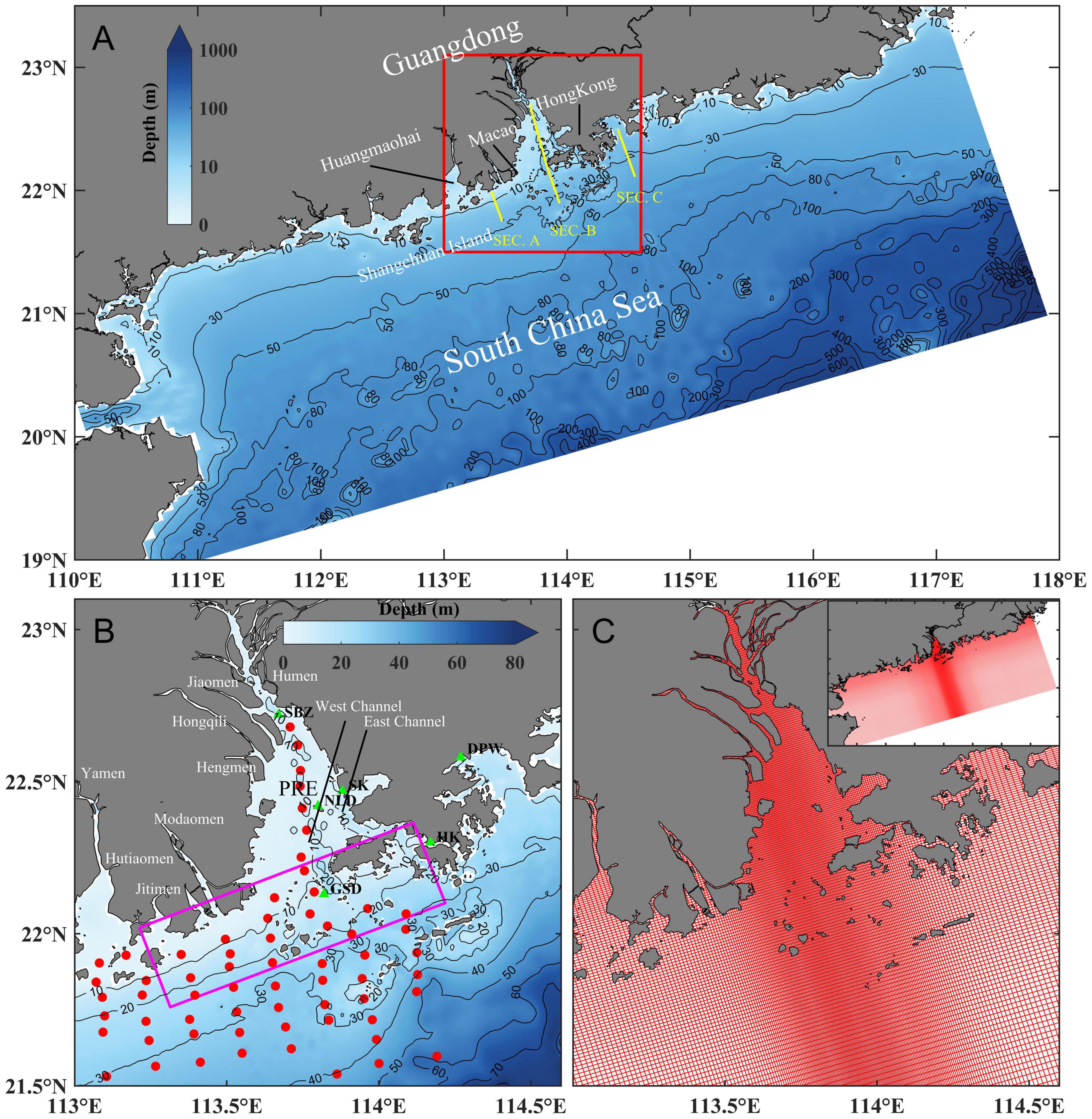
Figure 1. (A) Map and bathymetry of the Pearl River Estuary and the ambient water. (B) Zoomed-in view of the bathymetry of the Pearl River Estuary, with the names of major outlets labeled. (C) Numerical model domain and grid. Three yellow lines in panel (A) denote sections used in later analysis. Magenta box in panel (B) is a coastal transition zone [modified from Li et al. (2020)]. Red dots and green triangles in panel (B) denote cruise stations and tide gauges, respectively (SBZ = Shanbanzhou, SK = Shekou, NLD = Neilingding, GSD = Guishandao, DPW = Dapengwan, HK = Hongkong). The solid black lines in panel (A,B) are isobaths.
River plume features a low-salinity signature, and the surface water generally converges toward the front (Orton and Jay, 2005). Hence, the front often acts as a dynamic barrier to impede momentum and terrestrial materials from reaching the ocean. The structure of river plume fronts can be categorized into two types: surface-advected and bottom-trapped (Yankovsky and Chapman, 1997). The surface-advected plume floats over denser shelf water in a thin layer, with little contact with the bottom. Whereas a bottom-trapped plume forms a front from the surface to the bottom with a strong horizontal gradient, and its front is usually fixed at a depth deeper than the inflow depth. Previous studies have shown that bottom-trapped plume is influential in ecological processes. For example, the surface chlorophyll maximum near the estuary often occurs inside the salinity front (Franks, 1992), with a shoreward boundary at the location of the bottom front in turbid water (Wang et al., 2019). A large number of nutrients and pollutants carried by the river enter the Pearl River Estuary and extend in the shelf water along with the plume, which increases the nearshore productivity and produces a chlorophyll maximum zone at the front of the Pearl River Estuary (Hu and Li, 2009; Lu and Gan, 2015; Su et al., 2017). Stratification and multiple biogeochemical processes associated with the Pearl River plume also lead to the formation of hypoxic zones (Cui et al., 2019; Li et al., 2020). The spatial patterns of the high-value chlorophyll zone and the hypoxic zone in the Pearl River Estuary are closely related to the surface and bottom fronts of the Pearl River plume (Tang et al., 2003; Cui et al., 2019).
Numerous studies have been conducted on the Pearl River plume regarding its dynamics. Periodically variable runoff, monsoons and tides are recognized as important driving forces, which feature significant seasonal variability in the Pearl River. The summertime runoff is ∼20,000m3/s in June and July but drops to < 5,000m3/s in January and February (Figure 2). The Pearl River Estuary region is affected by the East Asian Monsoon, with the southwesterly wind prevailing in summer and the northeasterly wind prevailing in winter (Figure 2). The tidal range outside the entrance of the Pearl River Estuary is ∼2 m during spring tide but increases gradually to ∼3 m from the entrance to the upper reaches. Due to the seasonal changes of these external forces (particularly the runoff and wind), the extension of the Pearl River plume shows significant seasonal variations. In winter, the Pearl River plume extends along the west coast under the northeasterly monsoon. However, in summer, its mainstream extends offshore to the east coast under the upwelling-favorable wind, but a small portion still extends to the west coast (Wong et al., 2003). Ou et al. (2007) categorized the summer Pearl River plume into four types according to the horizontal salinity distribution: offshore bulge spreading, westward alongshore spreading, eastward offshore spreading, and westward-eastward bidirectional alongshore spreading. Some studies have suggested that the coastal current driven by the seasonal monsoon causes the variation of the plume (Wong et al., 2003; Ou et al., 2009).
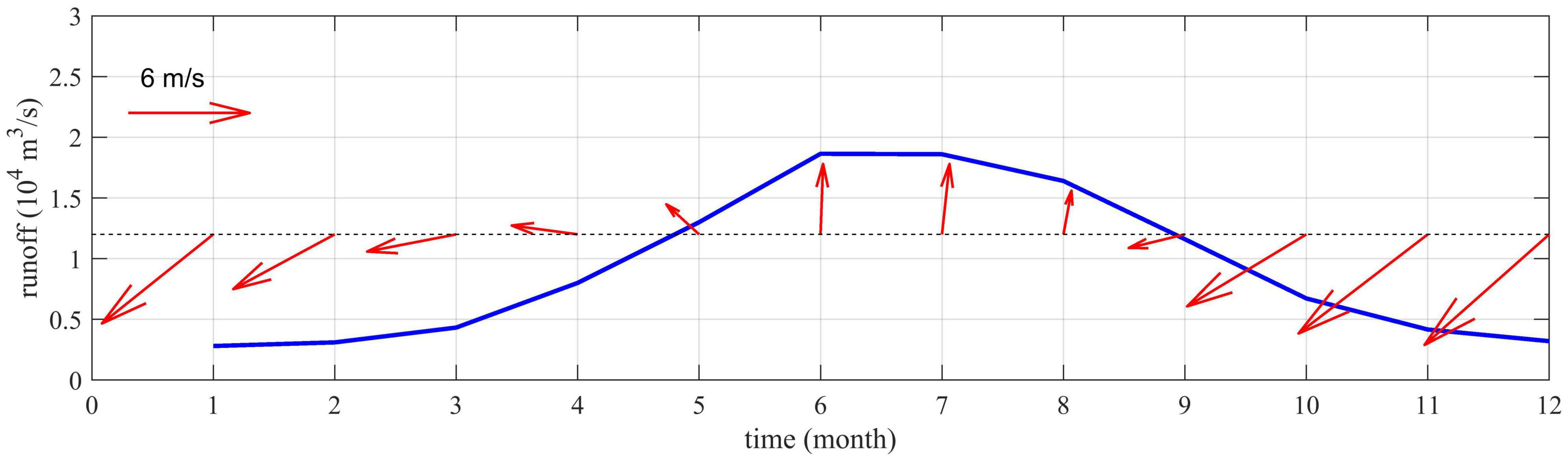
Figure 2. Climatological monthly averaged runoff and wind vectors.
River plume dynamics have been explored extensively (e.g., Yankovsky and Chapman, 1997; Garvine, 1999; Lentz, 2001; Fong and Geyer, 2002; Whitney and Garvine, 2005; Moffat and Lentz, 2012; Molinas et al., 2014). The mixing and extension of the Pearl River plume under these external forces have also received extensive attention. Luo et al. (2012) suggest that runoff affects the size of the plume extension, while monsoon determines the shape and position of the plume. Zu and Gan (2009, 2015) and Zu et al. (2014) studied the impact of tide, runoff, and wind on the Pearl River plume from the perspective of energy and momentum balances. These studies indicate that tide hinders the extension of the plume, whereas the coastal currents driven by the monsoon cause the seasonal shift in its extension direction. In addition, these studies suggested that the primary energy source is the tide inside the estuary, whereas, on the shelf, it turns to the wind. The tidal mixing increases the thickness of freshwater but weakens the surface wind-induced Ekman transport (Zu et al., 2014). Pan et al. (2014) calculated tidal salt deficit flux and found its magnitude is related to tide strength, while its direction is affected by the wind.
It should be pointed out that previous studies mainly focused on the river plume in the surface layer. However, the role of the bottom plume front was rarely mentioned. In fact, some studies implied that the Pearl River plume could be locked by topography. For instance, the hypoxia areas associated with the Pearl River plume are distributed along specific topography (see Figure 1), which is recognized as the coastal transition zone (Li et al., 2020). Studies in other regions (e.g., Wang et al., 2019) suggest that such a topographic lock of phytoplankton bloom and associated environmental consequences can be linked to the bottom front. Hence, in this study, we investigated the spatiotemporal characteristics of bottom and surface fronts of the Pearl River plume, as well as its underlying dynamics, based on a validated numerical model. The remainder of this paper is organized as follows. In Section “Materials and Methods,” the observed data, numerical model, and model validations are presented. The temporal and spatial characteristics of the surface and bottom front of the Pearl River plume are analyzed in Section “Results.” These characteristics are based on statistical methods of front occurrence probability and Empirical Orthogonal Function. In Section “Discussion,” dynamic factors that affect the plume front are discussed. Finally, we summarize our findings in section “Summary”.
Materials and Methods
Numerical Model
In this study, the Regional Ocean Modeling System (ROMS) (Shchepetkin and Mcwilliams, 2005) was configured with the model domain covering the Pearl River Estuary and its adjacent shelf (Figure 1A). The horizontal grid resolution was 500–800 m in the Pearl River Estuary and increased to 3–6 km in the open ocean. The eastern and western boundaries were perpendicular to the isobaths, while the southern boundary was located near the shelf break. The observed water depth data provided by Southern Marine Science and Engineering Guangdong Laboratory (Zhuhai) combined with the ETOPO2 data were interpolated to the model grids. A terrain-following S-coordinate (Song and Haidvogel, 1994) with 20 vertical levels was configured, and the surface and bottom layers were refined. A third-order HSIMT advection scheme developed by Wu and Zhu (2010) was selected for tracer advection simulation. Mellor and Yamada’s level 2.5 turbulent closure scheme (Mellor and Yamada, 1982) and Smagorinsky scheme (Smagorinsky, 1963) were used to parameterize vertical mixing and horizontal mixing. The model was initialized with climatologic temperature and salinity from the Ocean General Circulation Model for the Earth Simulator (OFES) data. Open boundary conditions of temperature, salinity and shelf current were also obtained from OFES data. Thirteen tide constituents (M2, S2, N2, K2, K1, O1, P1, Q1, MF, MM, MN4, M4, and MS4) extracted from Oregon State University (OSU) global inverse tidal model of TPXO8 (Egbert and Erofeeva, 2002) were used to provide tidal current and elevation for the open boundary. According to the diversion ratio suggested by Lu et al. (2013), the Pearl River runoff was distributed at eight major outlets. The atmospheric parameters (wind, air temperature, relative humidity, surface air pressure, cloud cover and net shortwave radiation) were provided by the European Centre for Medium-Range Weather Forecast (ECMWF) products (ERA-5 for realistic experiment and ERA-Interim for climatological experiment). The climatological experiment was driven by climatological monthly mean data of runoff, open boundary conditions, and atmospheric parameters. It was spun up for one year, and results of the second year were output for analysis. The configuration of the realistic experiment for model validation was the same as that of the climatological model except it was driven by 6-h atmospheric parameters.
Observed Data
Observed elevation and salinity data were used to validate the model. The elevation data used for comparison was observed during January 2008 at tide gauge stations that are marked with green triangles in Figure 1B. The salinity data were measured by a cruise organized by the Southern Marine Science and Engineering Guangdong Laboratory (Zhuhai). The cruise was conducted in the Pearl River Estuary and the adjacent shelf region from July 6 to 13, 2020. The sampling stations (as shown in Figure 1B) spanned from the Pearl River Estuary to the Huangmaohai and reached offshore to ∼50-m isobath.
Model Validation
Tides in the Pearl River Estuary and the adjacent water feature irregular semi-diurnal characteristics. K1, O1, M2 and S2 are the dominant tidal constituents in the NSCS, of which M2 is the strongest. Harmonic analysis was conducted for observed and modeled elevation data to obtain the amplitude and phase of different tidal constituents. The vectorial difference (Foreman et al., 1993) was then used to compare the modeled results with the observation:
in which a0 and g0 are the observed harmonic tidal amplitude and phase, and am and gm are the modeled counterparts. To normalize the results, the vectorial difference was further divided by the amplitude:
The results of vectorial difference are listed in Table 1. The mean Diff of M2 of all stations was 8.08 cm, and the mean Rdiff was 15.91%. The model simulated the M2 constituent reasonably. The Diff of S2 and K1 were 5.73 cm and 7.35 cm, respectively, and the associated Rdiff did not exceed 25%. Rdiff of O1 was 26.53% higher than other tidal constituents, but its absolute value was small given the small O1 amplitude. Among the six tide gauge stations, the simulation at Shanbanzhou, located at the upper estuary inside the Humen, showed the largest error. The Rdiff of three harmonic tides (O1, M2 and S2) exceeded 30% at this tide station. The tide in the river mouth is deformed to a certain extent, increasing the difficulty in accurate simulations. Given that the focus of this study was on the plume region, we did not further improve the validations. The overall model accuracy of simulating the tide was comparable with previous studies (e.g., Zu et al., 2014).
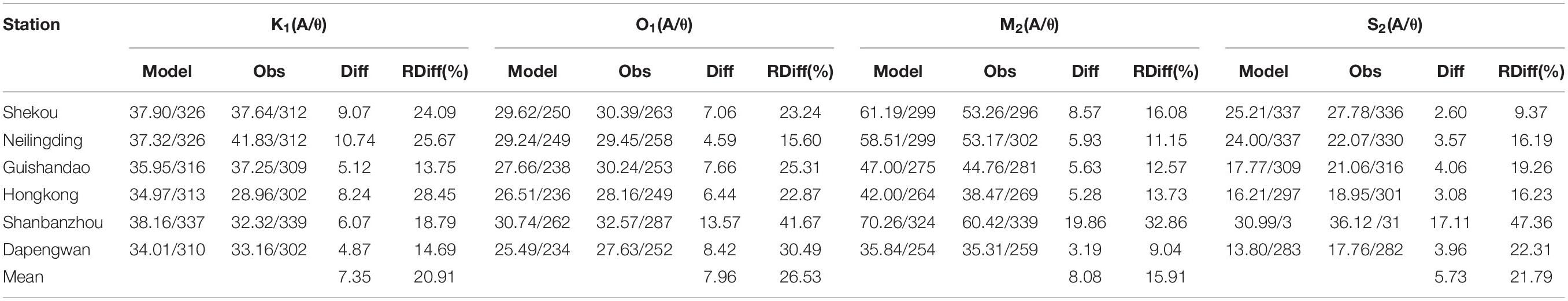
Table 1. Comparison between the modeled and observed amplitude (A in cm) and phase (θ in deg) of four major tide constituents of K1, O1, M2 and S2.
Observed data during July 2020 showed there was a low-salinity tongue outside the Pearl River Estuary (Figure 3A) and some researchers signify that the phenomenon is correlated to the West Channel geometry, estuarine outflow, tide, and wind (Pan et al., 2014; Liu et al., 2020). The surface plume extended in both directions to the east and west simultaneously (Figure 3A). The output data from the realistic forcing was compared with the observation (Figures 3B,D), showing reasonable skill in simulating the structure of the Pearl River plume both at the surface and the bottom. Inside the Pearl River Estuary, the shelf water intrusion simulated by the model was slightly weaker. Also, the modeled salinity near the Huangmaohai was relatively lower than the observation (Figures 3C,D). The reason could be that the model’s runoff releasing position was too close to the ocean, resulting in insufficient mixing before leaving the estuary. Other than these two areas, the modeled salinity distribution was close to the observed data. Model performance was quantified via the correlation coefficient (CC), the root-mean-square error (RMSE), and the skill score (SS). These metrics were calculated as follows:
in which X is the variable of interest and is its mean. Model performance was categorized as excellent when SS ≥ 0.65, very good when 0.65 > SS ≥ 0.5, good when 0.5 > SS ≥ 0.2, and poor when SS < 0.2 (Maréchal, 2004; Allen et al., 2007). Although RMSE was greater than 3, the CC exceeded 0.9 and the SS was 0.8 in both the surface and bottom layers (Figures 3E,F). The relatively large RMSE but excellent CC and SS were caused by the strong spatial variability of salinity in the Pearl River Estuary. Therefore, the model was reliable and can be used for further investigation.
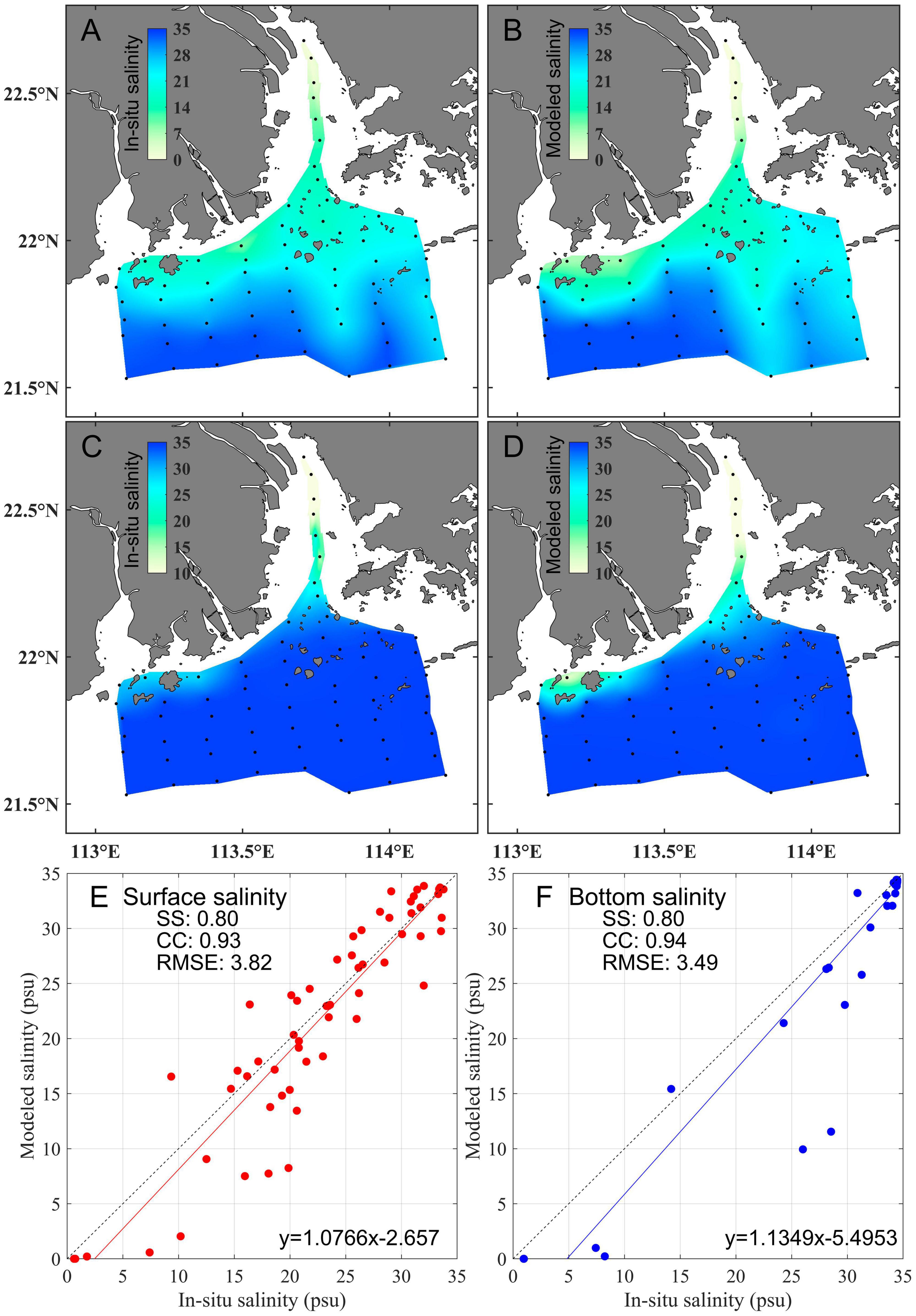
Figure 3. Validation of the surface and bottom salinity during July 2020 (dots signify the sampling stations). (A,C) are surface and bottom observed salinity, respectively. (B,D) are modeled results, respectively. Scatterplots of model salinity and observed salinity are plotted in (E,F).
Results
Variation of the Pearl River Plume
According to previous studies (Ou et al., 2009; Zu et al., 2014), the 32-psu isohaline can roughly denote the horizontal boundary of the Pearl River plume. We used the 75-h tidal-averaged salinity during the spring tides in different seasons to represent the seasonal variation of salinity distributions (Figure 4). In summer, as the runoff increased, the freshwater gradually extended outside the river mouth, and the prevailing southwesterly wind drove the coastal current to the northeast. The plume was thus brought to the eastern side of Pearl River Estuary. However, a portion of the plume extended toward the west coast simultaneously. The bottom plume, however, did not turn as did the surface. The bottom plume front existed only on the west coast of the Pearl River Estuary in summer, indicating that the plume extension to the east was surface-advected and that the extension to the west was bottom-trapped. The plume completely extended to the west in winter when the wind turned northeasterly. Its width was narrower than in summer. There were also seasonal variations inside the Pearl River Estuary. In summer, the surface plume filled the entire estuary, and the bottom shelf water intruded landward along two deep channels. In winter, the plume accumulated to the western side of the Pearl River Estuary, and the bottom shelf water intrusion that occupied the east side of the estuary was even more robust.
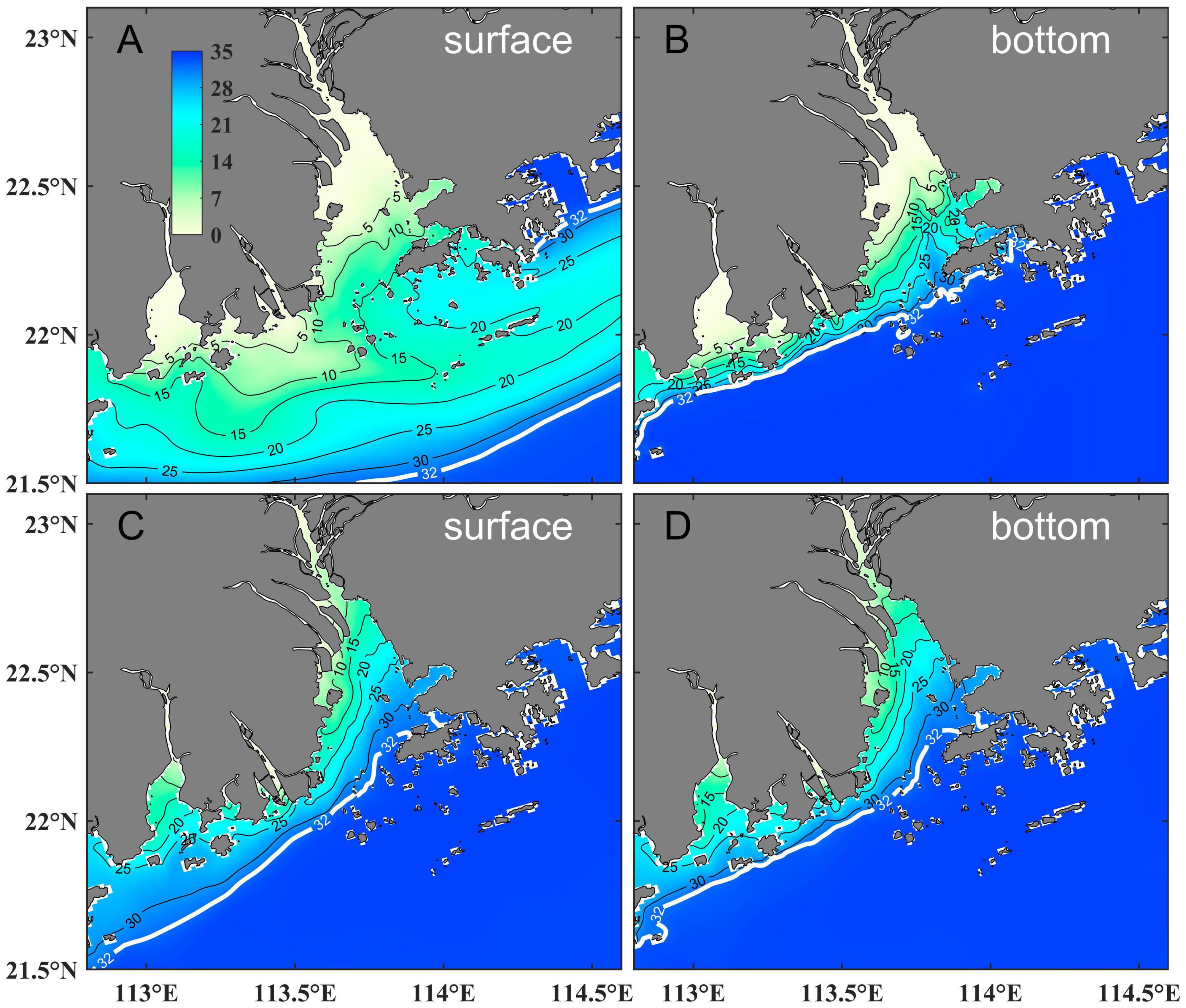
Figure 4. Tidal-averaged surface and bottom salinity in summer (A,B) and winter (C,D) during spring tides. The solid black lines are isohaline and the 32-psu isohaline is highlighted by the thick white line.
Whitney and Garvine (2005) suggested a wind index , in which Uwind≈2.65×10⁻²U, , U is along-shelf wind speed (up-shelf direction is positive in this study), K is internal Kelvin number, is the reduced gravity, ρ0 is ambient seawater density, ρr is the freshwater density, Q is the runoff, and f is the Coriolis parameter. Ws quantifies the relative importance of wind stress and the down-shelf buoyancy-driven current. |Ws| less than one indicates that the buoyancy-driven current is stronger than the wind-driven current. The calculated |Ws| was ∼0.3 in summer but > 1 in winter. The existence of plume water along the west coast and the fact |Ws| < 1 in summer indicated that the extension of the Pearl River plume was controlled not only by the wind, but also by its baroclinicity.
The profile of Section A (Figures 5A–D) indicates that the river plume was bottom-trapped to the west of the Pearl River Estuary in summer and winter. The isohaline in winter was much sparser and more vertical than in summer. The isohaline during the spring tide was more vertical than during the neap tide. There was strong stratification in Section B in summer with a significant surface-to-bottom salinity difference. In winter, the isohaline in Section B was nearly vertical and the stratification was weakened significantly. In summer, the plume extended to the east coast under the upwelling-favorable summer monsoon (Figures 5I,J). A brackish water mass appeared in the offshore region as influenced by the surface-advected plume. In winter, Section C was occupied by high salinity water.
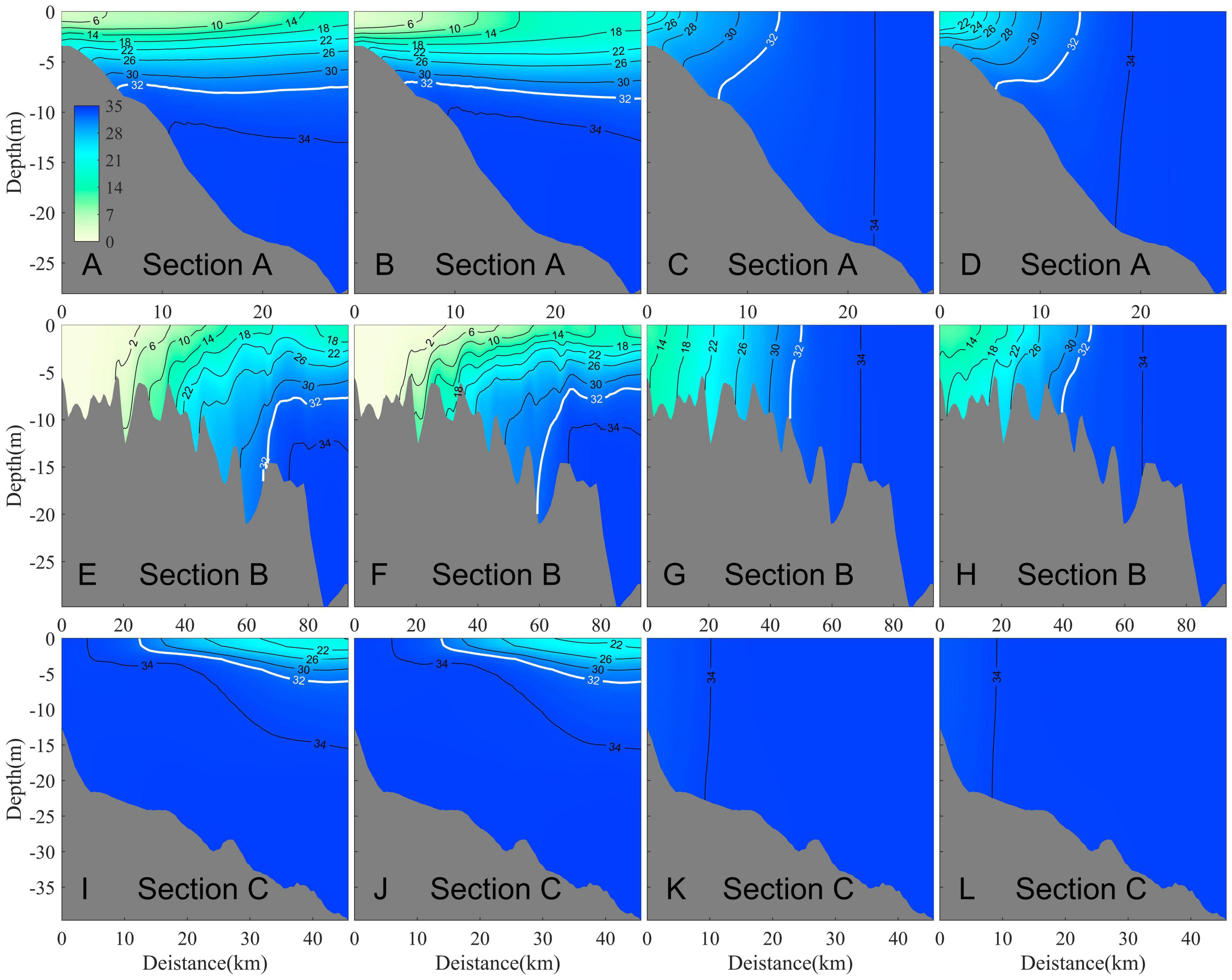
Figure 5. Tidal-averaged salinity on the cross-shelf transections during the spring tide (A,C,E,G,I,K) and the neap tide (B,D,F,H,J,L) in summer (A,B,E,F,I,J) and winter (C,D,G,H,K,L), respectively. The top row is section A, the middle is section B and the bottom is section C. The solid black lines are isohaline and the 32-psu isohaline is highlighted by the thick white line.
Salinity Gradient and Occurrence Probability of the Front
It is evident that the spatiotemporal variations of the Pearl River plume were very drastic. The surface-to-bottom salinity difference was also considerable in summer (Figure 5; later further shown in Figure 13A). Therefore, it is important to choose an appropriate method to describe the variability of the plume.
The gradient method is often used to identify fronts (Huang et al., 2010; He et al., 2016; Wu and Wu, 2018). In this study, the salinity gradient magnitude (SGM) was used to calculate the gradient in the surface and bottom layers of the Pearl River Estuary and its adjacent waters:
In which ΔS1 and ΔS2 are the diagonal salinity difference of a 3 × 3 grid, while ΔX1 and ΔX2 are the diagonal distance between corners of the corresponding grids. The hourly modeled salinity was used to calculate SGM and then averaged over the period of interest. The seasonal and spring-neap cycles of the front are the main focus of this study. Annual-mean salinity gradient was used to indicate the average position of the front (Figures 6A,B). The surface salinity gradient in most areas of the model domain was small except in the Modaomen, Huangmaohai and Pearl River Estuary (Figure 6A). The bottom salinity gradient in the Pearl River Estuary and its adjacent coastal water was concentrated in a narrow region shoreward of ∼10-m isobath with a value up to 2 psu/km (Figure 6B). The distribution of the high bottom salinity gradient basically followed along the coastline. The standard deviation of the surface salinity gradient was large because the surface plume was affected by wind stress. Whereas in the bottom, the standard deviation of the salinity gradient was small, indicating the bottom plume front was more stable.
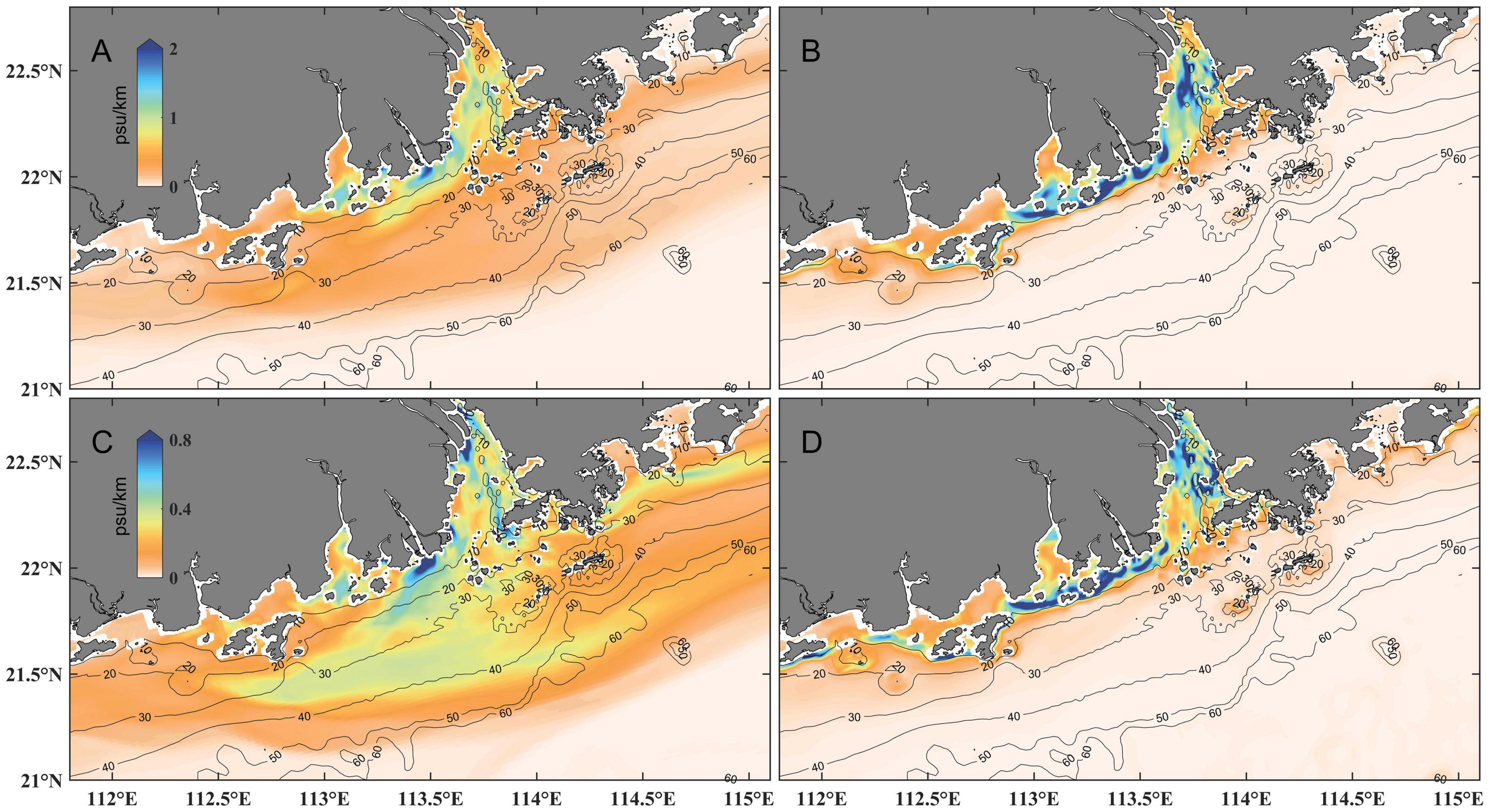
Figure 6. Annual-averaged surface (A) and bottom (B) salinity gradient (A,B) and its standard deviation (C,D). The solid black lines indicate isobaths.
Summer (June to August) and winter (December to the next February) are flood and dry seasons, respectively. Therefore, these two seasons were selected as typical seasons to explore the cross-shelf variation in salinity gradients in Sections A, B, and C (Figure 7). The bottom front did not exist in Section C but occurred in Section A and Section B in winter and summer. Both the surface front and the bottom front had variations in intensity and spatial position. The bottom salinity gradients in Section A and Section B were stronger in summer than in winter on the seasonal scale. The surface and bottom front extended seaward in summer but shrank shoreward in winter. The seasonal cross-shelf movement of the surface front has a migration scale of ∼2 km in Section A and ∼20 km in Section B. The seasonal cross-shelf movement of the bottom front was smaller than that of the surface one, with Section A being ∼1.2 km and Section B being ∼10 km. In spring-neap tide cycles, the cross-shelf movement of the surface front was not obvious in Section B, although the phenomenon was apparent in Section A. The bottom front had a stronger intensity during the neap tides than during the spring. This was due to the increase of the tide mixing in the spring tide inducing more vigorous shear dispersion that decreased the horizontal gradient. There were three extreme values on the bottom front at Section B and their positions correspond to the bathymetric variations. The bottom front moved seaward during the spring tides and landward during the neap tides. The migration scale of the bottom front in neap-spring cycles in Section A was ∼0.8 km in summer and ∼0.4 km in winter. The migration scale in neap-spring cycles in Section B was relatively larger than in Section A with ∼3 km in summer and ∼1 km in winter, respectively. The migration of the front depends not only on the strength of the external forces but also on the seafloor slope. According to the Yankovsky and Chapman (1997) theory, under the same external force, the greater the seafloor slope the smaller the horizontal migration distance of the front.
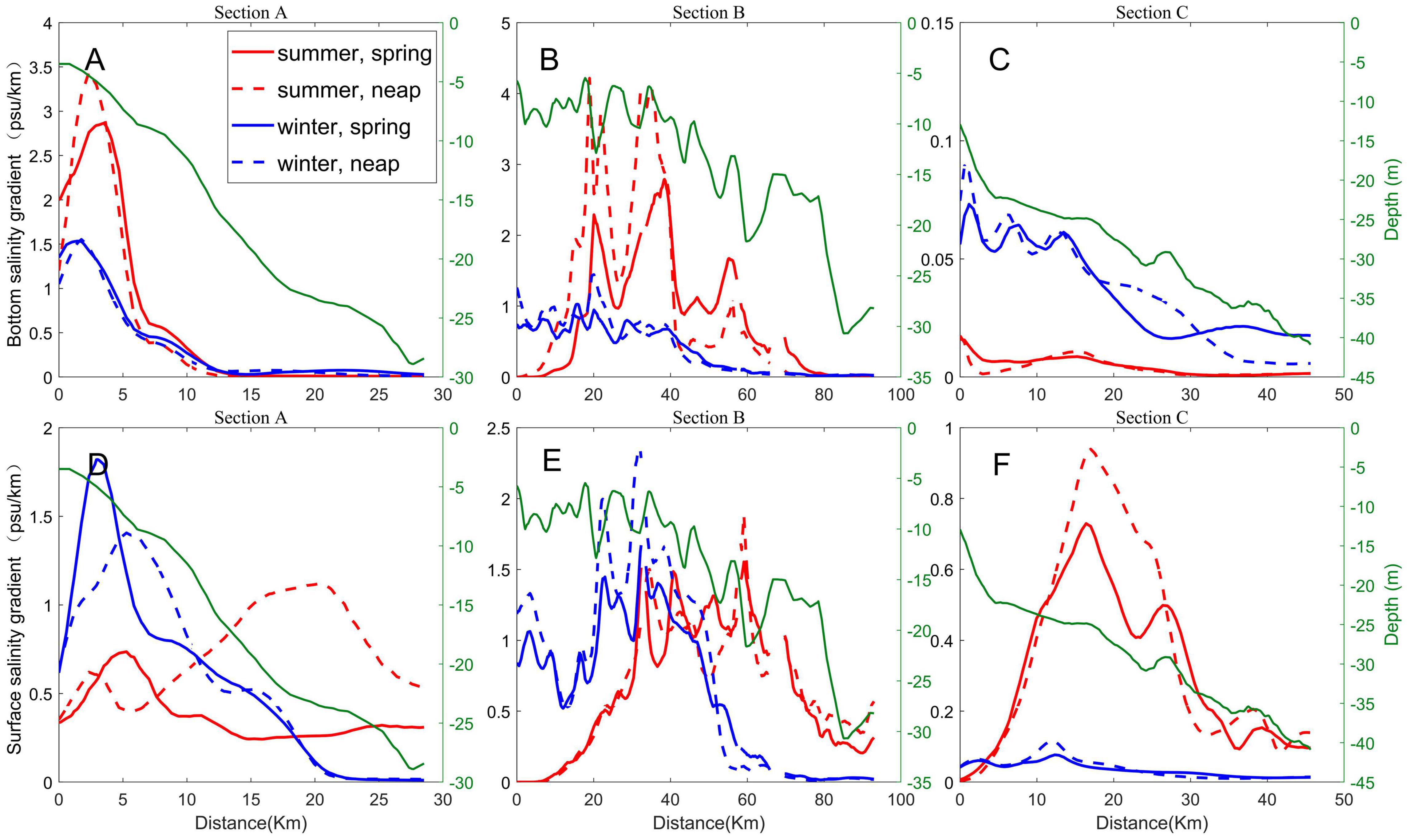
Figure 7. Tidal-averaged cross-shelf bottom salinity gradient in Section A (A,D), Section B (B,E) and Section C (C,F) during spring tide and neap tide in winter (December) and summer (July), respectively. The top row is for the bottom layer, and the bottom row is for the surface layer, respectively. Red and blue colors indicate results in summer and winter, respectively. Green lines signify section depth. Solid and dotted lines represent results in spring tide and neap tide, respectively.
The annual-mean salinity gradient and its standard deviation (Figure 6) provided basic information of the Pearl River plume front. However, averaging over a long-time span may obscure the actual intensity of the front. Therefore, we further calculated the occurrence probability of the plume front when its intensity exceeded a given threshold. Fedorov threshold (Fedorov, 1986)-i.e., ten times the average salinity gradient in the study area- was often used to detect the front (Fedorov, 1986). However, it should be noted that the Fedorov threshold is sensitive to the domain selected. To reflect the position of the front in different seasons more reasonably, we choose 0.8 psu/km as the threshold according to Figure 7. Counting the time of which the salinity gradient is greater than 0.8psu/km in the four seasons, and then dividing it by the total time span, we got the occurrence probability of the salinity front (Figure 8) in four seasons (i.e., spring, summer, autumn and winter). In summer, the surface front existed in the east coast and moved offshore significantly; hence, there was a large area with a noticeable occurrence probability. The surface front also existed in the offshore region in spring and autumn; however, the probability dropped to ∼10%. In winter, the surface salinity front entirely extended to the west coast. In this period, the coastal extension of the front is the shortest, shrinking to the position around 113°E.
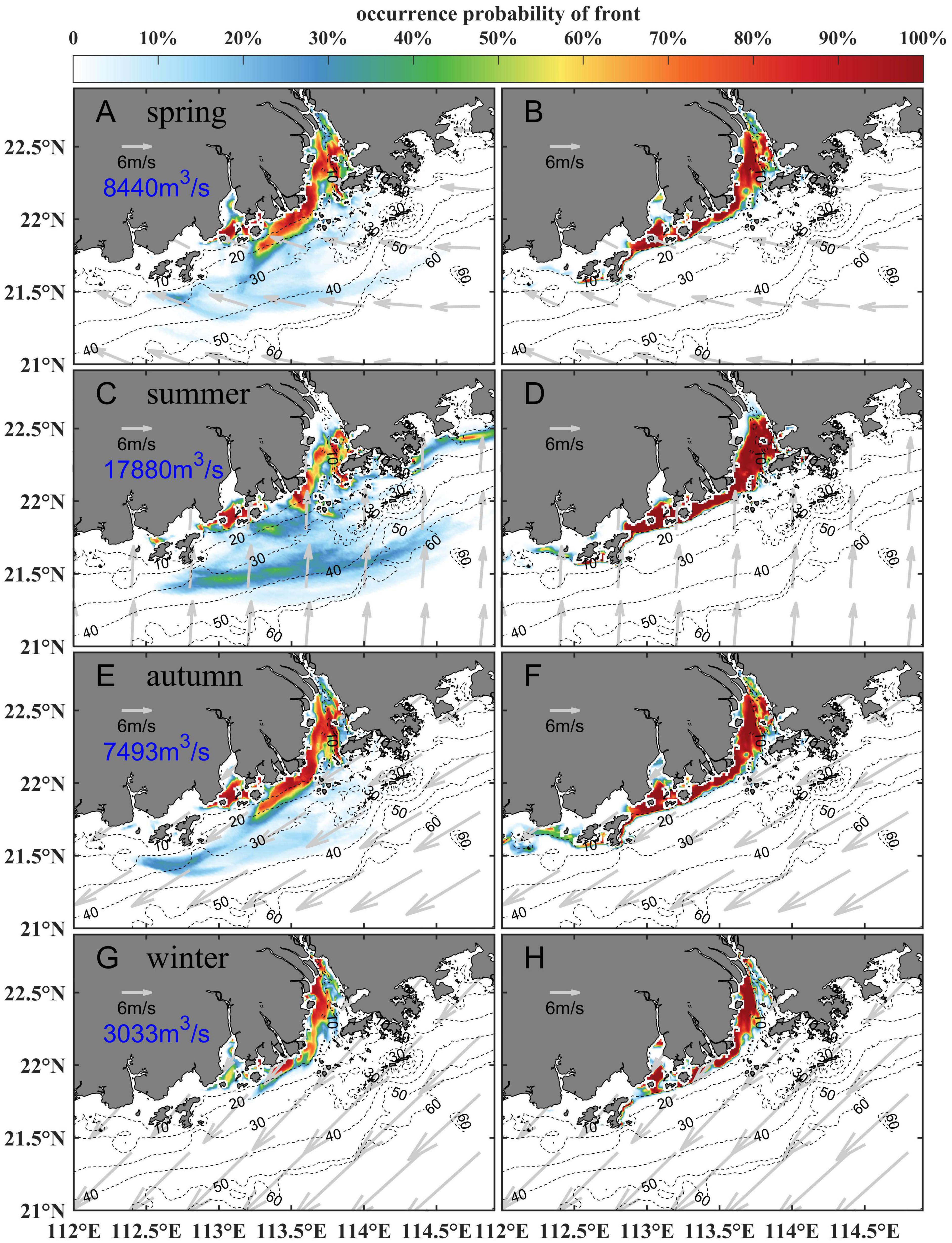
Figure 8. Seasonal occurrence probability of surface (A,C,E,G) and bottom (B,D,F,H) fronts in spring (A,B), summer (C,D), autumn (E,F), and winter (G,H), respectively. The left column is the surface layer, and the right column is the bottom layer. Seasonal mean runoff and wind field are also labeled. The black dotted lines are isobaths.
Whereas for the bottom front, the high occurrence probability area was distributed in a more narrow region and was nearly identical throughout four seasons (Figure 8). This indicated that the bottom front was strongly “rooted” on the seafloor. The occurrence of the surface front in the west region opposite to the wind direction in summer could be closely linked to the formation of the bottom front, as indicated by previous studies (e.g., Wu and Wu, 2018).
Empirical Orthogonal Function Analysis
To infer the formation dynamics of such a stable bottom front, the variability of the bottom salinity gradient was further analyzed by the EOF method. Before doing the EOF, the bottom salinity gradient was low-pass filtered (with a cut-off window of 72 h) to remove the strong intra-tidal signal, and then the long-term mean was further subtracted from the data. Hence, EOF analysis was performed on the anomaly field of the bottom salinity gradient. The results are shown in Figure 9. The three leading EOF modes contributed 58.7%, 13.9% and 7.8% of the total variance, respectively, totaling 80.4%, which represented most of the variance in the bottom salinity gradient in the Pearl River Estuary.
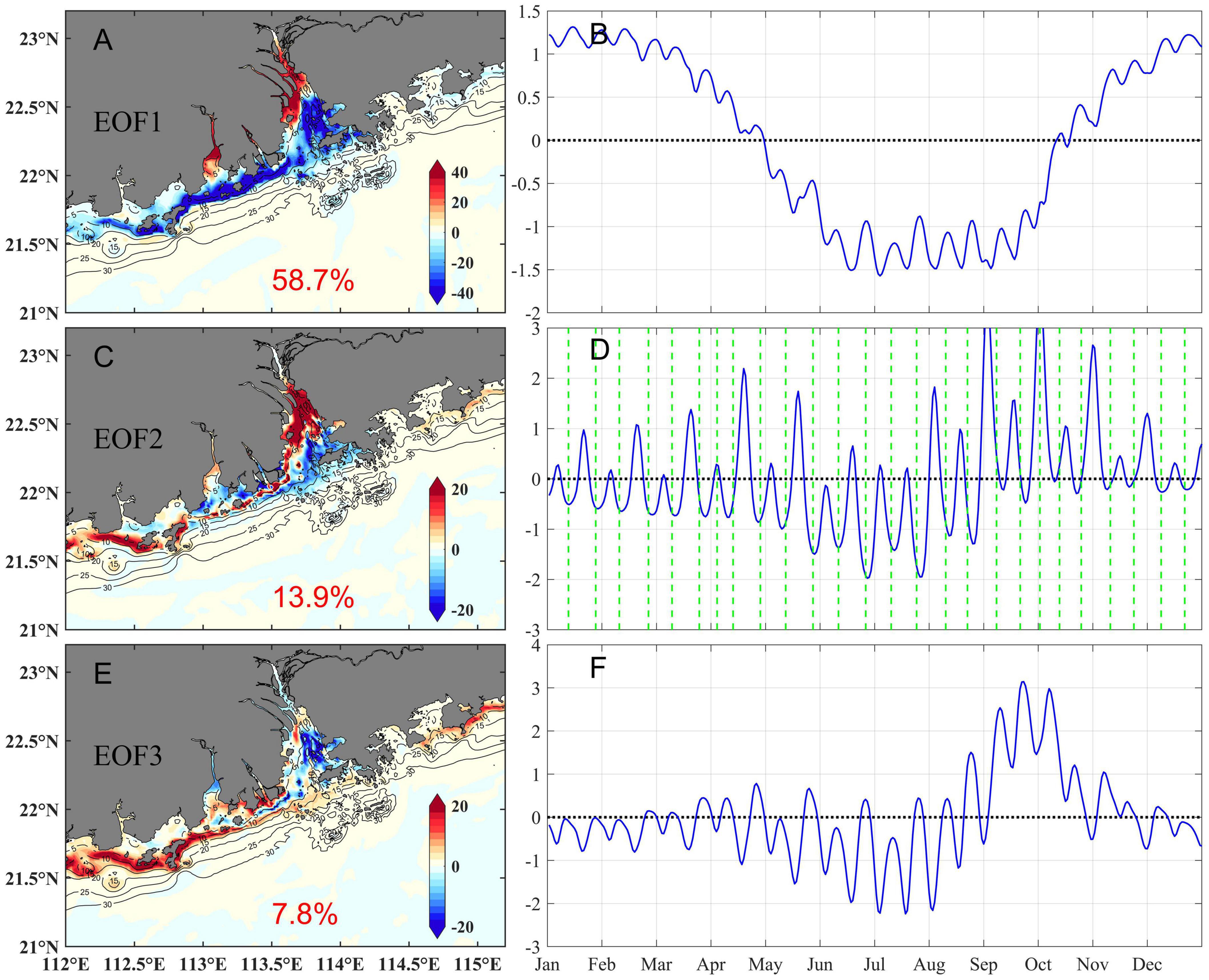
Figure 9. Three leading EOF modes [Mode 1: (A,B); Mode 2: (C,D); Mode3: (E,F)] of the bottom salinity gradient. The green dotted lines in panel (D) denote the spring tides. The solid black lines (A,C,E) are isobaths.
Mode 1 showed a notable seasonal variation of the bottom front. During the spring and winter seasons, the bottom front shrank toward the coast, but it moved toward the sea during the summer and autumn seasons. This mode was mainly related to runoff and along-shelf wind with a correlation coefficient of -0.95 and -0.87, respectively. In summer and autumn, the runoff was large; meanwhile, the bottom front moved toward the sea. Correspondingly, the runoff was small in spring and winter, and the bottom front moved toward the land.
Mode 2 indicated a significant spring-neap cross-shelf movement. The correlation coefficient between Mode 2 and the tidal range was -0.57. The bottom front moved seaward during the spring tide, whereas it moved shoreward during the neap tides. It can also be seen that the influence of tide on the bottom front was the strongest in August and September, in consistence with the amplification of the tidal range around the autumnal equinox. West of ∼113.5°E, the spatial mode was different from that on the east side because there were freshwater sources from other tributaries of the estuary.
Mode 3, which contributed to the total variance less significantly, peaked during September and October. Its correlations with wind, runoff or tidal forcing were not as apparent as previous two modes. We inferred it was caused by the transition of the summer plume to the winter plume. In summer, a large area of river plume was surface advected due to the large river discharge and the upwelling-favorable summer monsoon. Then in autumn, the remainder of this plume was transported to the west coast, which supplied excess plume water that favored the formation of a strong bottom front.
Discussion
Momentum Balance
Momentum terms from the model were used to diagnose the dynamic characteristics of the Pearl River plume. The average momentum terms over 75 h were used to remove tidal oscillations. The coordinate was rotated to represent the along-shelf (x) and cross-shore (y) directions.
The tidal-averaged momentum equation across the shelf reads:
in which the tidal-averaging operator was omitted. The terms on the right-hand side are the advection, Coriolis force, barotropic pressure gradient force, baroclinic pressure gradient force, and vertical friction force, respectively. The horizontal diffusion term was neglected because it was much smaller than the vertical diffusion.
Results across Section A during the spring tide in summer and winter seasons are shown in Figure 10. The barotropic pressure gradient force was seaward (positive value) and the baroclinic pressure gradient force was landward (negative value). The total pressure gradient force and Coriolis force were largely balanced in the cross-shelf direction. This momentum balance in winter was more in line with the thermal wind balance than in summer. The advection term also has larger values on the surface layers and at the top of the bottom boundary layer, indicating strong nonlinearity. The vertical friction of the surface layer was strong in summer, and the friction of the bottom boundary layer was strong in winter. Overall, the momentum balance was more geostrophic in the winter season, while the nonlinear momentum advection and friction became important in summer. This was apparently related to the different front shapes in these two seasons. Nevertheless, from Figure 10, it is clear that the locations associated with maximum bottom salinity gradient were similar in winter and summer, regardless of contrast dynamic balances. This seems consistent with the dynamics of EOF mode 2. The cross-shelf location was controlled by tidal forcing, which remains largely unchanged during different seasons.
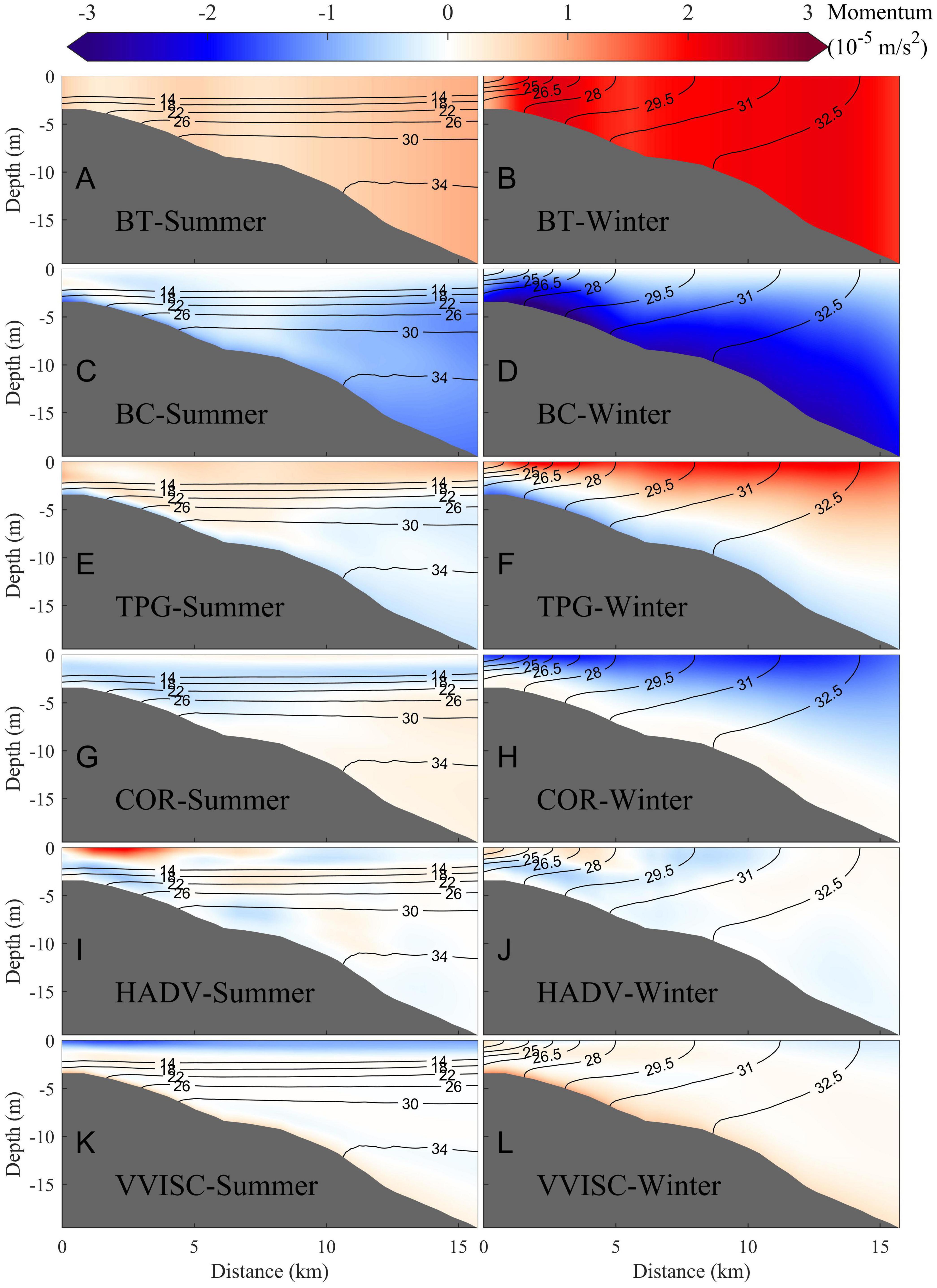
Figure 10. Cross-shelf component of tidal-averaged momentum terms in Section A during summer (July) and winter (January) spring tides, respectively. (A,B) barotropic pressure gradient force; (C,D) baroclinic pressure gradient force; (E,F) total pressure gradient force; (G,H) Coriolis force; (I,J) horizontal momentum advection; (K,L) vertical turbulent viscous term. The solid black lines are isohalines.
Tidal Modulation on the River Plume
The EOF analysis, as well as the above momentum balance analysis, indicated that tide was a dominant forcing determining the cross-shelf position of the bottom front. This, however, was in contrast to the previous conclusion that was derived from a non-tidal river plume (Chapman and Lentz, 1994; Yankovsky and Chapman, 1997). In these studies, the cross-shelf position was controlled by river discharge and wind through the bottom Ekman dynamics.
Hence, a sensitivity experiment with tide excluded was configured to further explore the role of the tide in controlling the bottom front in the Pearl River Estuary. The average surface salinity in April and the entire spring season are shown in Figure 11. The model results showed that dramatic differences can be found with tidal forcing removed. In the absence of tide, the Pearl River plume also extended to the upstream, in consistence with the findings in other estuaries (e.g., Guo and Valle-Levinson, 2007; Wu et al., 2011). With tide included, the surface plume extended further to the sea.
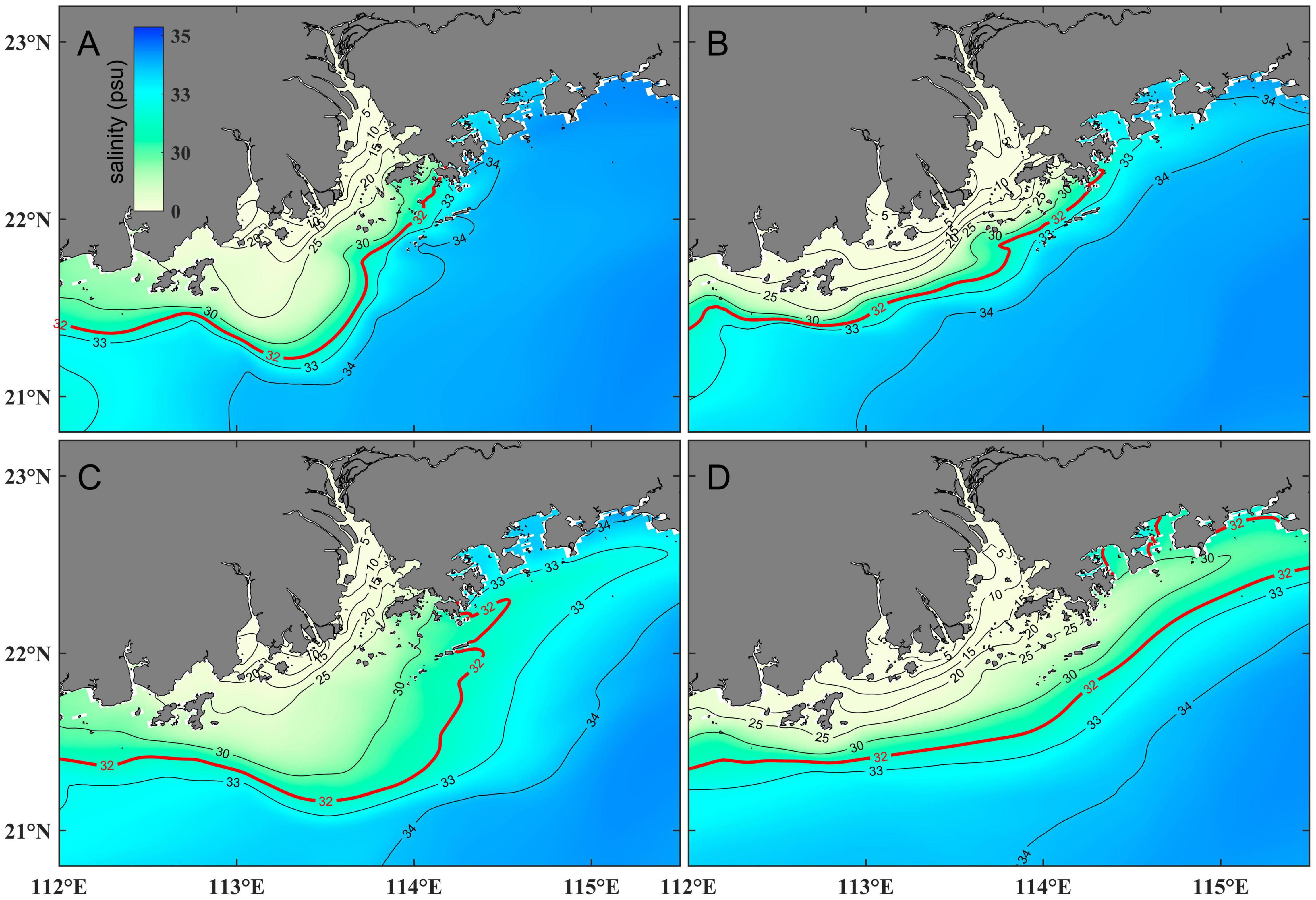
Figure 11. Averaged surface salinity in April (A,B) and the entire spring season (C,D) with (A,C) and without (B,D) tide, respectively. The solid black lines are isohaline and the 32-psu isohaline is highlighted by the thick red line.
The difference between tidal and non-tidal simulations in all four seasons is shown in Figure 12. The bottom 32-psu contour was roughly located along the line connecting Macao and Hong Kong in the tide’s presence. In the absence of tide, a large amount of shelf water intruded into the Pearl River Estuary, hence, the bottom front moved shoreward. This was due to the enhanced estuarine circulation under weak mixing, thus strong stratification (Gong et al., 2018). The difference in the 32-psu contours in the shelf region was small between the two sensitivity experiments, indicating that the impact of the tide on the front weakened in the offshore region.
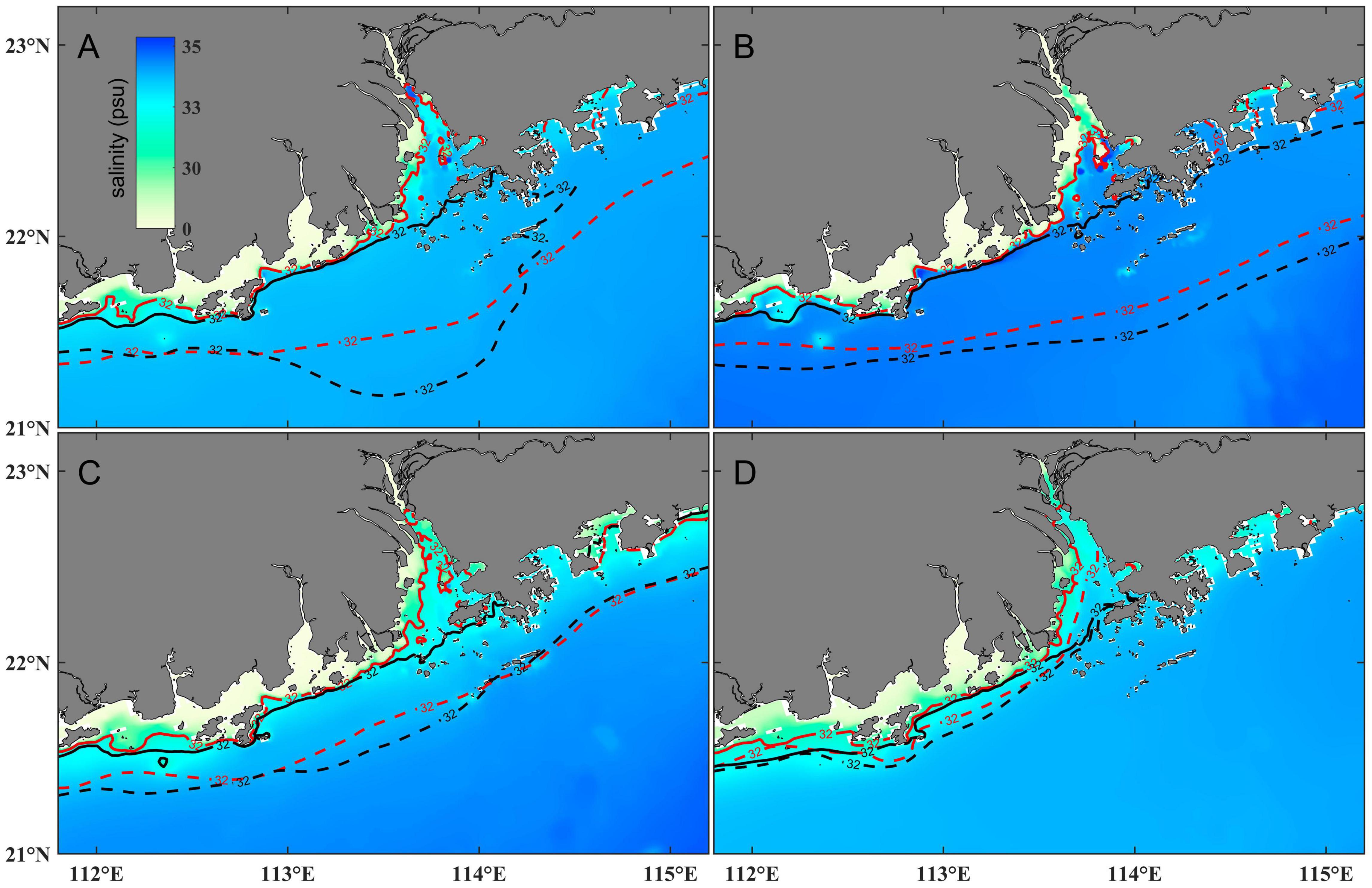
Figure 12. Distribution of the bottom salinity in the presence and absence of tide in spring (A), summer (B), autumn (C) and winter (D), respectively. The color shading is the salinity in the absence of tide, the dashed and solid lines are the 32-psu contours in the surface layer and the bottom layer, respectively. The black lines and red lines denote the result with and without tide, respectively.
The spring-neap migration of the bottom front implied that it could be linked to the tidal front due to differential mixing over topography (Simpson and Hunter, 1974; Wu and Wu, 2018). Simpson-Hunter (SH) number can be used to compare the relative strength of the mixing caused by tidal current and by stratification (Simpson and Hunter, 1974),
in which h is the water depth, UT is the maximum tidal velocity during the spring tide. The smaller the SH number is, the more likely the tidal mixing can overcome vertical stratification. An SH number between 1.7 and 2 was commonly taken as the position of the tidal-induced mixing front (Beardsley et al., 1985; Loder and Greenberg, 1986; Wu and Wu, 2018). As shown in Figure 13B, the SH number in the Pearl River Estuary was less than 2, indicating that tide could thoroughly mix the entire water column. In the coastal area from the entrance of the Pearl River Estuary to the west coast, SH number value was between 1.7 and 2. Thus, there was a boundary between stratified and mixed waters at the entrance of the Pearl River Estuary. This place was consistent with the region with a high occurrence probability of the bottom front (Figure 7). This indicated that the formation and maintenance of the bottom plume front were closely linked to the tidal mixing, which was similar to the Changjiang River plume (Wu and Wu, 2018).
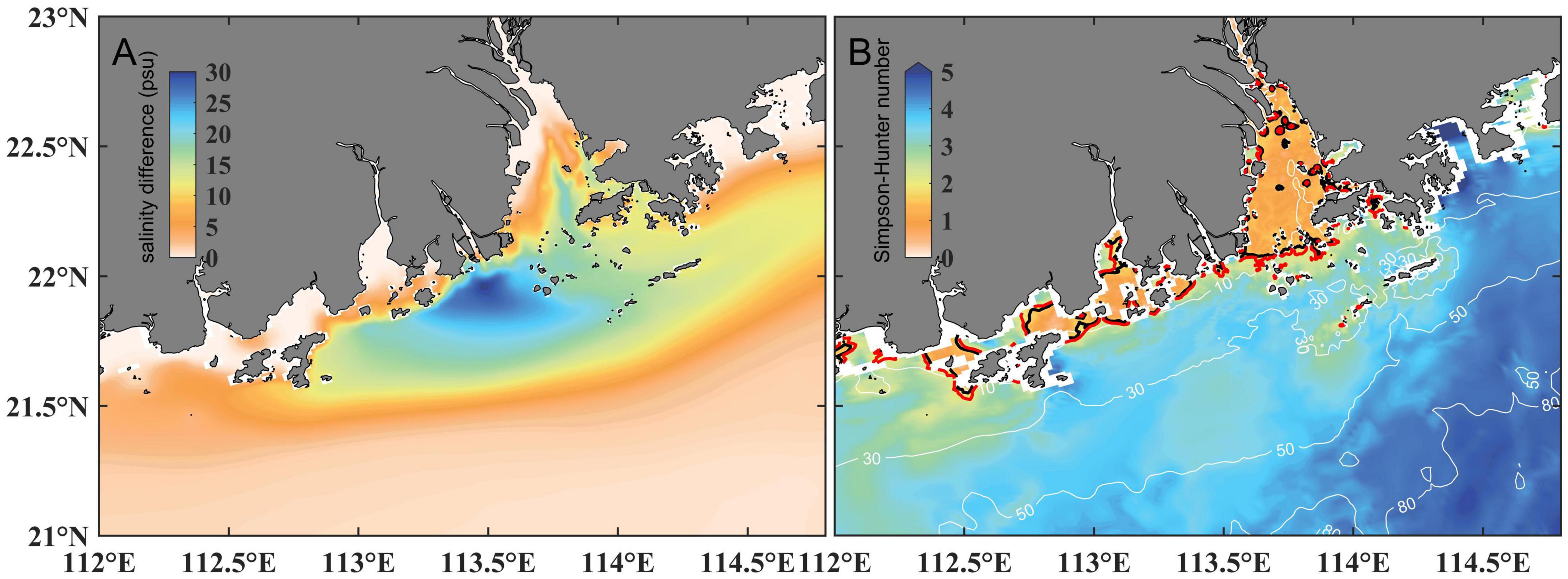
Figure 13. Averaged surface-to-bottom salinity difference during the entire summer season (A) and the distribution of Simpson-Hunter number (B). The black and red solid lines in (B) are the contours of SH = 1.7 and SH = 2, respectively.
Summary
A numerical model with high resolution in the Pearl River Estuary was configured to explore the spatiotemporal distribution of the Pearl River plume front. The model validation indicated that it can reasonably reproduce the structure of the Pearl River plume. The salinity gradient magnitude and the occurrence probability of the front were used to identify the mean and standard deviation of the plume front both at the surface and the bottom. The results indicated that a year-round bottom front existed in the Pearl River Estuary and the west coast, while the surface front was much more variable. The spatial position of the Pearl River plume front is summarized in Figure 14.
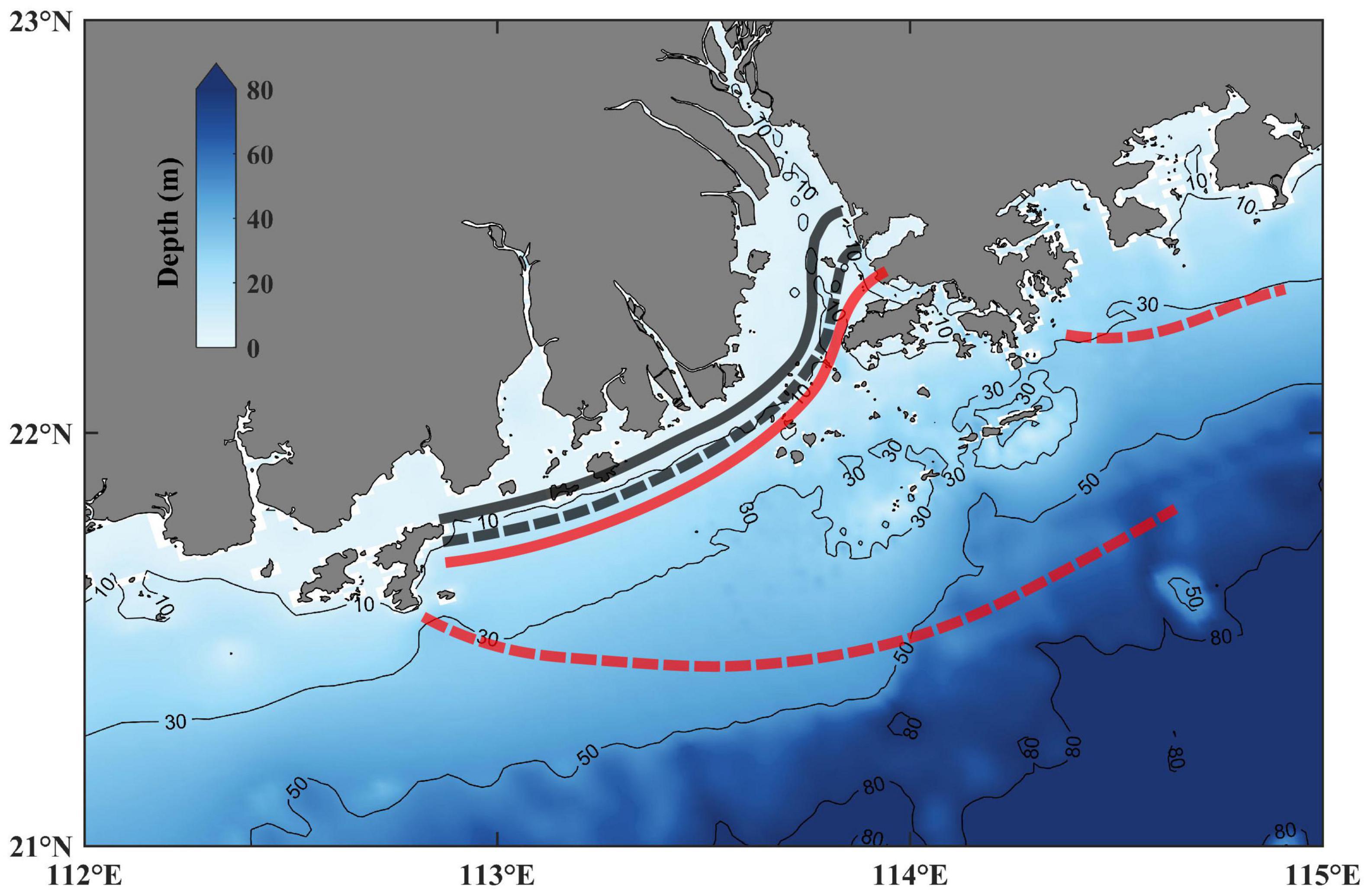
Figure 14. Schematic map of the spatiotemporal distribution of the front. The solid thick lines are the bottom front position, and the dashed thick lines are the surface front position, respectively. The red color and black color represent summer and winter seasons, respectively. The solid black lines signify the isobaths.
Empirical Orthogonal Function (EOF) analysis indicated that the Pearl River discharge was the primary external forcing regulating the bottom front intensity. With a larger discharge, the bottom front became stronger and moved seaward. Additionally, the tide was a significant factor affecting the cross-shelf position of the bottom front, moving to the sea during the spring tides but to the land during the neap tides. The cross-shelf movement of the bottom front was more pronounced in August and September, consistent with the amplification of the tidal range around the autumnal equinox. Momentum analysis signified that the Coriolis force and the total pressure gradient force balance dominated in the study region, and the nonlinear advection term and friction term became important in summer.
Experiments with and without tide were further conducted to explore the tidal influence on the Pearl River plume front. In the absence of tides, the river plume also extended to the upstream even though the wind was not upwelling-favorable, and the bottom front moved landward. It can be seen from the Simpson-Hunter number that tide can overcome the influence of stratification, causing differential mixing over topography, thus producing a tidal front that sustained the Pearl River plume front. Consequently, the Pearl River plume front was rooted on the seafloor, which should be essential for the frequent occurrence of hypoxia in certain areas.
Data Availability Statement
The raw data supporting the conclusions of this article will be made available by the authors, without undue reservation.
Author Contributions
HW designed the research. HZ conducted the numerical experiments and wrote the first draft of the manuscript. HZ and YW analyzed the results. All authors contributed extensively to the interpretation of results and approved the submitted version.
Funding
This study was supported by Innovation Group Project of Southern Marine Science and Engineering Guangdong Laboratory (Zhuhai) (Grant No. 311020003), the Innovation Program of Shanghai Municipal Education Commission (Grant Nos. 2021-01-07-00-08-E00102), the National Natural Science Foundation of China (Grant Nos. 42106162 and 41776101).
Conflict of Interest
The authors declare that the research was conducted in the absence of any commercial or financial relationships that could be construed as a potential conflict of interest.
Publisher’s Note
All claims expressed in this article are solely those of the authors and do not necessarily represent those of their affiliated organizations, or those of the publisher, the editors and the reviewers. Any product that may be evaluated in this article, or claim that may be made by its manufacturer, is not guaranteed or endorsed by the publisher.
References
Allen, J. I., Somerfield, P. J., and Gilbert, F. J. (2007). Quantifying uncertainty in high-resolution coupled hydrodynamic-ecosystem models. J. Mar. Syst. 64, 3–14. doi: 10.1016/j.jmarsys.2006.02.010
Beardsley, R. C., Limeburner, R., Yu, H., and Cannon, G. A. (1985). Discharge of the Changjiang (Yangtze River) into the East China Sea. Cont. Shelf Res. 4, 57–76. doi: 10.1016/0278-4343(85)90022-6
Chapman, D. C., and Lentz, S. J. (1994). Trapping of a coastal density front by the bottom boundary layer. J. Phys. Oceanogr. 24, 1464–1479.
Cui, Y. S., Wu, J. X., Ren, J., and Xu, J. (2019). Physical dynamics structures and oxygen budget of summer hypoxia in the Pearl River Estuary. Limnol. Oceanogr. 64, 131–148. doi: 10.1002/lno.11025
Dong, L. X., Su, J. L., Wong, L. A., Cao, Z. Y., and Chen, J. C. (2004). Seasonal variation and dynamics of the Pearl River plume. Cont. Shelf Res. 24, 1761–1777. doi: 10.1016/j.csr.2004.06.006
Egbert, G. D., and Erofeeva, S. Y. (2002). Efficient inverse modeling of Barotropic Ocean tides. J. Atmos. Ocean. Technol. 19, 183–204. doi: 10.1175/1520-0426(2002)019<0183:eimobo>2.0.co;2
Fedorov, K. N. (1986). The Physical Nature and Structure of Oceanic Fronts. New York, NY: Springer-Verlag.
Fong, D. A., and Geyer, W. R. (2002). The alongshore transport of freshwater in a surface-trapped river plume*. J. Phys. Oceanogr. 32, 957–972.
Foreman, M. G. G., Henry, R. F., Walters, R. A., and Ballantyne, V. A. (1993). A finite element model for tides and resonance along the north coast of British Columbia. J. Geophys. Res. 98, 2509–2531. doi: 10.1029/92JC02470
Franks, P. J. S. (1992). Phytoplankton blooms at fronts: patterns, scales, and physical forcing mechanisms. Rev. Aquat. Sci. 6, 121–137.
Gan, J. P., Li, L., Wang, D. X., and Guo, X. G. (2009). Interaction of a river plume with coastal upwelling in the northeastern South China Sea. Cont. Shelf Res. 29, 728–740. doi: 10.1016/j.csr.2008.12.002
Garvine, R. W. (1995). A dynamical system for classifying buoyant coastal discharges. Cont. Shelf Res. 15, 1585–1596. doi: 10.1016/0278-4343(94)00065-U
Garvine, R. W. (1999). Penetration of buoyant coastal discharge onto the continental shelf: a numerical model experiment. J. Phys. Oceanogr. 29, 1892–1909. doi: 10.1175/1520-048519990292.0.CO
Gong, W. P., Lin, Z. Y., Chen, Y. Z., Chen, Z. Y., and Zhang, H. (2018). Effect of winds and waves on salt intrusion in the Pearl River estuary. Ocean Sci. 14, 139–159. doi: 10.5194/os-14-139-2018
Guo, X. Y., and Valle-Levinson, A. (2007). Tidal effects on estuarine circulation and outflow plume in the Chesapeake Bay. Cont. Shelf Res. 27, 20–42. doi: 10.1016/j.csr.2006.08.009
He, S. Y., Huang, D. J., and Zeng, D. Y. (2016). Double SST fronts observed from MODIS data in the East China Sea off the Zhejiang–Fujian coast, China. J. Mar. Syst. 154, 93–102. doi: 10.1016/j.jmarsys.2015.02.009
Hu, J. T., and Li, S. Y. (2009). Modeling the mass fluxes and transformations of nutrients in the Pearl River Delta, China. J. Mar. Syst. 78, 146–167. doi: 10.1016/j.jmarsys.2009.05.001
Huang, D. J., Zhang, T., and Zhou, F. (2010). Sea-surface temperature fronts in the Yellow and East China Seas from TRMM microwave imager data. Deep Sea Res. II Top. Stud. Oceanogr. 57, 1017–1024. doi: 10.1016/j.dsr2.2010.02.003
Lai, Z. G., Ma, R. H., Gao, G. Y., Chen, C. S., and Beardsley, R. C. (2015). Impact of multichannel river network on the plume dynamics in the Pearl River estuary. J. Geophys. Res. Oceans 120, 5766–5789. doi: 10.1002/2014JC010490
Lentz, S. J. (2001). The influence of stratification on the wind-driven cross-shelf circulation over the North Carolina Shelf*. J. Phys. Oceanogr. 31, 2749–2760.
Li, D., Gan, J. P., Hui, R., Liu, Z. Q., Yu, L. Q., Lu, Z. M., et al. (2020). Vortex and biogeochemical dynamics for the hypoxia formation within the coastal transition zone off the Pearl River estuary. J. Geophys. Res. Oceans 125:e2020JC016178. doi: 10.1029/2020JC016178
Liu, X. C., Gu, Y. Z., Li, P. L., Liu, Z. Z., Zhai, F. G., and Wu, K. J. (2020). A tidally dependent plume bulge at the Pearl River Estuary mouth. Estuar. Coast. Shelf Sci. 243:106867. doi: 10.1016/j.ecss.2020.106867
Loder, J. W., and Greenberg, D. A. (1986). Predicted positions of tidal fronts in the Gulf of Maine region. Cont. Shelf Res. 6, 397–414. doi: 10.1016/0278-4343(86)90080-4
Lu, L. Y., Zhan, J. M., and Geng, B. X. (2013). Study of the Pearl River plume dispersion based on flux budget analysis [in Chinese]. J. Hydrodyn. 28, 252–259. doi: 10.3969/j.issn1000-4874.2013.03.002
Lu, Z. M., and Gan, J. P. (2015). Controls of seasonal variability of phytoplankton blooms in the Pearl River Estuary. Deep Sea Res. II Top. Stud. Oceanogr. 117, 86–96. doi: 10.1016/j.dsr2.2013.12.011
Luo, L., Zhou, W., and Wang, D. (2012). Responses of the river plume to the external forcing in Pearl River Estuary. Aquat. Ecosyst. Health Manage. 15, 62–69. doi: 10.1080/14634988.2012.655549
Maréchal, D. (2004). A Soil-Based Approach to Rainfall-Runoff Modeling in Ungauged Catchments for England and Wales. dissertation’s thesis. Bedford: Cranfield University.
Mellor, G. L., and Yamada, T. (1982). Development of a turbulence closure model for geophysical fluid problems. Rev. Geophys. 20, 851–875. doi: 10.1029/RG020i004p00851
Moffat, C., and Lentz, S. J. (2012). On the response of a buoyant plume to downwelling-favorable wind stress. J. Phys. Oceanogr. 42, 1083–1098. doi: 10.1175/JPO-D-11-015.1
Molinas, E., Vinzon, S. B., Vilela, C., and Gallo, M. N. (2014). Structure and position of the bottom salinity front in the Amazon Estuary. Ocean Dyn. 64, 1583–1599. doi: 10.1007/s10236-014-0763-0
Orton, P. M., and Jay, D. A. (2005). Observations at the tidal plume front of a high-volume river outflow. Geophys. Res. Lett. 32, 1–16. doi: 10.1029/2005GL022372
Ou, S. Y., Zhang, H., and Wang, D. X. (2007). Horizontal characteristics of buoyant plume off the Pearl River Estuary during summer. J. Coast. Res. SI 50, 652–657.
Ou, S. Y., Zhang, H., and Wang, D. X. (2009). Dynamics of the buoyant plume off the Pearl River Estuary in summer. Environ. Fluid Mech. 9, 471–492. doi: 10.1007/s10652-009-9146-3
Pan, J. Y., Gu, Y. Z., and Wang, D. X. (2014). Observations and numerical modeling of the Pearl River plume in summer season. J. Geophys. Res. Oceans 119, 2480–2500. doi: 10.1002/2013JC009042
Shchepetkin, A. F., and Mcwilliams, J. C. (2005). The regional oceanic modeling system (ROMS): a split-explicit, free-surface, topography-following-coordinate oceanic model. Ocean Model. 9, 347–404. doi: 10.1016/j.ocemod.2004.08.002
Simpson, J. H., and Hunter, J. R. (1974). Fronts in the Irish Sea. Nature 250, 404–406. doi: 10.1038/250404a0
Smagorinsky, J. (1963). General circulation experiments with the primitive equations. J. Mon. Weather Rev 91, 99–164. doi: 10.1115/1.4027610
Song, Y., and Haidvogel, D. (1994). A semi-implicit ocean circulation model using a generalized topography-following coordinate system. J. Comput. Phys. 115, 228–244. doi: 10.1006/jcph.1994.1189
Su, J. Z., Dai, M. H., He, B. Y., Wang, L. F., Gan, J. P., Guo, X. H., et al. (2017). Tracing the origin of the oxygen-consuming organic matter in the hypoxic zone in a large eutrophic estuary: the lower reach of the Pearl River Estuary, China. Biogeosciences 14, 1–24. doi: 10.5194/bg-2017-43
Tang, D. L., Kester, D. R., Ni, I. H., Qi, Y. Z., and Kawamura, H. (2003). In situ and satellite observations of a harmful algal bloom and water condition at the Pearl River estuary in late autumn 1998. Harmful Algae 2, 89–99. doi: 10.1016/S1568-9883(03)00021-0
Wang, S. F., Tang, D. L., He, F. L., Fukuyo, Y., and Azanza, R. V. (2008). Occurrences of harmful algal blooms (HABs) associated with ocean environments in the South China Sea. Hydrobiologia 596, 79–93. doi: 10.1007/s10750-007-9059-4
Wang, Y. H., Wu, H., Gao, L., Shen, F., and Liang, X. S. (2019). Spatial distribution and physical controls of the spring algal blooming off the Changjiang river estuary. Estuar. Coasts 42, 1066–1083. doi: 10.1007/s12237-019-00545-x
Whitney, M. M., and Garvine, R. W. (2005). Wind influence on a coastal buoyant outflow. J. Geophys. Res. Oceans 110:C03014. doi: 10.1029/2003JC002261
Wong, L. A., Chen, J. C., Xue, H., Dong, L. X., Guan, W. B., and Su, J. L. (2003). A model study of the circulation in the Pearl River Estuary (PRE) and its adjacent coastal waters: 2. Sensitivity experiments. J. Geophys. Res. Oceans 108:3157. doi: 10.1029/2002JC001452
Wu, H., and Zhu, J. R. (2010). Advection scheme with 3rd high-order spatial interpolation at the middle temporal level and its application to saltwater intrusion in the Changjiang Estuary. Ocean Model. 33, 33–51. doi: 10.1016/j.ocemod.2009.12.001
Wu, H., Zhu, J. R., Shen, J., and Wang, H. (2011). Tidal modulation on the Changjiang River plume in summer. J. Geophys. Res. Oceans 116:C08017. doi: 10.1029/2011JC007209
Wu, T. N., and Wu, H. (2018). Tidal mixing sustains a bottom-trapped river plume and buoyant coastal current on an energetic continental shelf. J. Geophys. Res. Oceans 123, 9061–9081. doi: 10.1029/2018JC014105
Yankovsky, A. E., and Chapman, D. C. (1997). A simple theory for the fate of buoyant coastal discharges. J. Phys. Oceanogr. 27, 1386–1401.
Yu, L. Q., Gan, J. P., Dai, M. H., Hui, C. R., Lu, Z. M., and Li, D. (2020). Modeling the role of riverine organic matter in hypoxia formation within the coastal transition zone off the Pearl River Estuary. Limnol. Oceanogr. 66, 452–468.
Zu, T. T., and Gan, J. P. (2009). Process-Oriented study of the river plume and circulation in the Pearl River estuary: response to the wind and tidal forcing. Adv. Geosci. 12, 213–230. doi: 10.1142/9789812836168_0015
Zu, T. T., and Gan, J. P. (2015). A numerical study of coupled estuary-shelf circulation around the Pearl River Estuary during summer: responses to variable winds, tides and river discharge. Deep Sea Res. II Top. Stud. Oceanogr. 117, 53–64. doi: 10.1016/j.dsr2.2013.12.010
Keywords: Pearl River Estuary, river plume, salinity gradient, bottom front, tide
Citation: Zhi H, Wu H, Wu J, Zhang W and Wang Y (2022) River Plume Rooted on the Sea-Floor: Seasonal and Spring-Neap Variability of the Pearl River Plume Front. Front. Mar. Sci. 9:791948. doi: 10.3389/fmars.2022.791948
Received: 09 October 2021; Accepted: 28 January 2022;
Published: 17 February 2022.
Edited by:
Alexander Yankovsky, University of South Carolina, United StatesReviewed by:
Gonzalo S. Saldías, University of the Bío Bío, ChileNadia K. Ayoub, UMR 5566 Laboratoire d’Études en Géophysique et Océanographie Spatiales (LEGOS), France
Copyright © 2022 Zhi, Wu, Wu, Zhang and Wang. This is an open-access article distributed under the terms of the Creative Commons Attribution License (CC BY). The use, distribution or reproduction in other forums is permitted, provided the original author(s) and the copyright owner(s) are credited and that the original publication in this journal is cited, in accordance with accepted academic practice. No use, distribution or reproduction is permitted which does not comply with these terms.
*Correspondence: Hui Wu, aHd1QHNrbGVjLmVjbnUuZWR1LmNu