 Kimberly T. Goetz1,2*
 Fabrice Stephenson3
 Andrew Hoskins4
 Aidan D. Bindoff5
 Rachael A. Orben6
 Paul M. Sagar7
 Leigh G. Torres8
 Caitlin E. Kroeger9Lisa A. Sztukowski10
 Richard A. Phillips11
 Stephen C. Votier12
 Stuart Bearhop12Graeme A. Taylor13David R. Thompson1
- 1National Institute of Water and Atmospheric Research, Wellington, New Zealand
- 2Marine Mammal Laboratory, Alaska Fisheries Science Center, National Marine Fisheries Service, National Oceanic and Atmospheric Administration (NOAA), Seattle, WA, United States
- 3National Institute of Water and Atmospheric Research, Hamilton, New Zealand
- 4The Commonwealth Scientific and Industrial Research Organisation (CSIRO) Health and Biosecurity, Townsville, QLD, Australia
- 5Wicking Dementia Research and Education Centre, University of Tasmania, Hobart, TAS, Australia
- 6Department of Fisheries, Wildlife, and Conservation Sciences, Hatfield Marine Science Center, Oregon State University, Newport, OR, United States
- 7National Institute of Water and Atmospheric Research, Christchurch, New Zealand
- 8Department of Fisheries, Wildlife, and Conservation Sciences, Marine Mammal Institute, Oregon State University, Newport, OR, United States
- 9Farallon Institute, Petaluma, CA, United States
- 10Commonwealth of the Northern Mariana Islands, Department of Lands and Natural Resources, Division of Fish and Wildlife, Saipan, MP, United States
- 11British Antarctic Survey, Natural Environmental Research Council, Cambridge, United Kingdom
- 12Centre for Ecology and Conservation, University of Exeter, Cornwall, United Kingdom
- 13Aquatic Unit, Department of Conservation, Wellington, New Zealand
Few studies have assessed the influence of data quality on the predicted probability of occurrence and preferred habitat of marine predators. We compared results from four species distribution models (SDMs) for four southern-hemisphere albatross species, Buller’s (Thalassarche bulleri), Campbell (T. impavida), grey-headed (T. chrysostoma), and white-capped (T. steadi), based on datasets of differing quality, ranging from no location data to twice-daily locations of individual birds collected by geolocation devices. Two relative environmental suitability (RES) models were fit using minimum and maximum preferred and absolute values for each environmental variable based on (1) monthly 50% kernel density contours and background environmental data, and (2) primary literature or expert opinion. Additionally, two boosted regression tree (BRT) models were fit using (1) opportunistic sightings data, and (2) geolocation data from bird-borne electronic tags. Using model-specific threshold values, habitat was quantified for each species and model. Model variables included distance from land, bathymetry, sea surface temperature, and chlorophyll-a concentration. Results from both RES models and the BRT model fit with opportunistic sightings were compared to those from the BRT model fit using geolocation data to assess the influence of data quality on predicted occupancy and habitat. For all species, BRT models outperformed RES models. BRT models offer a predictive advantage over RES models by being able to identify relevant variables, incorporate environmental interactions, and provide spatially explicit estimates of model uncertainty. RES models resulted in larger, less refined areas of predicted habitat for all species. Our study highlights the importance of data quality in predicting the distribution and habitat of albatrosses and emphasises the need to consider the pros and cons associated with different levels of data quality when using SDMs to inform management decisions. Furthermore, we examine the overlap in preferred habitat predicted by each SDM with fishing effort. We discuss the influence of data quality on predicting the wide-scale distributions of pelagic seabirds and how these impacts could result in different protection measures.
1 Introduction
Continuing declines in biodiversity have prompted local and international agencies to advocate for much-improved spatial protection measures in both terrestrial and marine environments (Tancell et al., 2016; Dias et al., 2017; Augé et al., 2018; Hays et al., 2019; Hindell et al., 2020). This goal, in conjunction with the increased availability of high resolution location data for flora and fauna, have led to the wider application of species distribution models (SDMs) for conservation (Johnson and Gillingham, 2005; Rodríguez et al., 2007; Franklin, 2010; Porfirio et al., 2014). The power of SDMs lies in converting point locations into predicted (spatially explicit) probability of occurrence and preferred habitat. SDMs have become widely used for understanding geographic range (Torres et al., 2008; Goetz et al., 2012), estimating extinction rates (Benito et al., 2009; Pliscoff et al., 2014; Stephenson et al., 2020), understanding impacts of climate change (Laidre et al., 2008; Kaschner et al., 2011), prioritizing biodiversity conservation (Moilanen et al., 2005; Oliveira et al., 2017; Fuentes‐Castillo et al., 2019), and planning the size and location of protected areas (Hooker et al., 1999; Gerrodette and Eguchi, 2011). Ideally, reliable records of presence/absence data collected during systematic surveys (in space and time) which encompass the full potential range of a species would be used in SDMs to examine the relationship between occurrence and the environment. However, high-quality location data are not available for most mobile species and the field studies required to obtain such information over large spatial-temporal scales are prohibitively expensive or logistically unfeasible. Consequently, SDMs are often informed with the best available data, which is likely to be limited in space and time and may necessitate collation of data from different sources, including opportunistic sightings (Derville et al., 2018). Alternatively, when little or no data are available, relative environmental suitability (RES) models have been used to predict species occurrence using qualitative descriptions from the literature or expert opinion (Kaschner et al., 2006; Watson et al., 2013; Stephenson et al., 2020).
For management purposes, predictions from SDMs are frequently extrapolated to areas well beyond the spatial-temporal range of the underlying data. This approach may be acceptable when the ecology of a species is well understood, the drivers of distribution change little from one area to another, or when long-term, high-quality data are used to predict species occurrence (Elith and Leathwick, 2009; Torres et al., 2015). However, when coverage of the data is insufficient, predictions may grossly over- or under-estimate occurrence and habitat use (Stockwell and Peterson, 2002; Elith et al., 2010), potentially resulting in protection measures that are inappropriate or ineffective (Rowden et al., 2019).
Technological advancements in bio-logging technology have led to an increased understanding of movement, foraging behaviour, and habitat use for some species (Block, 2005; Cooke, 2008; Evans et al., 2013; Wilmers et al., 2015). While bio-logging data is often considered the gold standard for understanding species distribution, in reality, high-quality data are often not available. Given resource limitations, management decisions for protected or threatened species, are frequently made on the basis of species distribution data that are far from complete. Under this paradigm, it is important to understand how results from SDMs informed with different types and quality of location data compare. In this study, we quantified and compared the predicted probability of occurrence and preferred habitat generated from SDMs informed by datasets of varying quality for Buller’s (Thalassarche bulleri), Campbell (T. impavida), grey-headed (T. chrysostoma), and white-capped (T. steadi) albatrosses (hereafter referred to as BUAL, CAAL, GHAL, and WCAL, respectively), both globally and within New Zealand’s (NZ) Exclusive Economic Zone (EEZ). Although two sub-species of BUAL are recognised in NZ (e.g. Robertson et al., 2017), in this study we refer exclusively to the southern sub-species T. bulleri bulleri.
Albatrosses are a highly threatened group of seabirds with distributions spanning entire ocean basins. Mortality from fisheries bycatch is a leading threat globally, and is a concern for the majority albatrosses breeding in NZ (Lewison and Crowder, 2003; Waugh et al., 2008; Anderson et al., 2011; Žydelis et al., 2011; Croxall et al., 2012; Jiménez et al., 2014). The International Union for the Conservation of Nature (IUCN) defines albatross (Family Diomedeidae) as the most threatened family of seabirds in the world with 17 of the 22 species currently listed as ‘Vulnerable’, ‘Endangered’, or ‘Critically Endangered’ (Tuck et al., 2011). BUAL and WCAL are currently classified as ‘Near Threatened’, CAAL as ‘Vulnerable’, and GHAL as ‘Endangered’ on the IUCN Red List of Threatened Species (IUCN, 2021). Under the NZ threat classification system (Robertson et al., 2017), GHAL and CAAL are classified as ‘Threatened – nationally vulnerable’, WCAL as ‘At risk – declining’ and BUAL as ‘At risk – naturally uncommon’. All four species breed in New Zealand and are included in the ‘Assessment of Risk of Commercial Fisheries to NZ Seabirds’ (Richard et al., 2020).
In this study, we quantify the differences in preferred habitat predicted by SDMs fit with data of varying quality for four species of southern hemisphere albatross. Additionally, we quantify the monthly spatial overlap of preferred habitat predicted by four SDMs with fishing effort both globally and within NZ’s EEZ as well as the overlap in total preferred habitat predicted by the top two performing models with global fishing effort for each species. We hypothesized that SDMs fit with geolocation data would perform better than those fit using opportunistic sightings or qualitative descriptions of habitat use extracted from the literature. We also hypothesized that overlap in preferred habitat predicted by SDMs not fit with empirical data would result in greater overlap in fishing effort than models fit with high quality location data. We discuss the validity and caveats of predicting wide-scale distributions of pelagic seabirds from models fit with data of varying quality. Additionally, we compare the best performing SDMs to those currently used by manages to assess the risk of commercial fisheries to NZ seabirds (Sharp, 2017; Richard et al., 2020).
2 Materials and Methods
2.1 Study Area
Due to the wide-ranging distributions of albatrosses, the study area extended around the world from ~30-80°S. Additionally, because BUAL, CAAL, GHAL, and WCAL breed at colonies within the NZ’s EEZ, results are also summarized within this boundary (Figure 1).
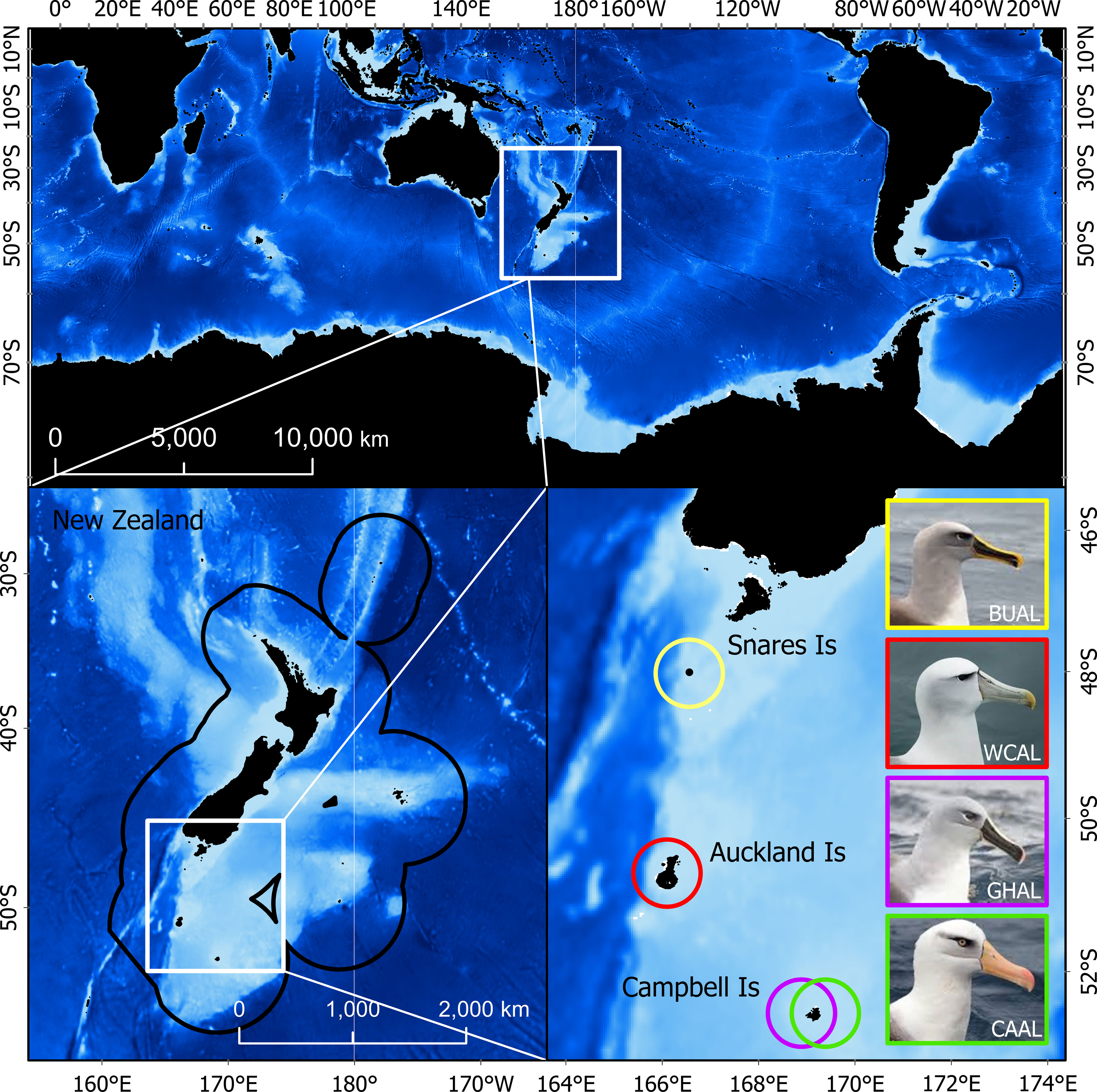
Figure 1 The study region in which probability of occurrence and habitat were predicted (top). The bottom panels show the tagging locations (breeding colonies) within the New Zealand Exclusive Economic Zone for four albatross species: Buller’s (BUAL), white-capped (WCAL), grey-headed (GHAL), and Campbell (CAAL).
2.2 Species Location Data
Opportunistic sightings contributed by citizen scientists through eBird were available for BUAL, CAAL, GHAL, and WCAL. eBird is an online, publicly accessible database (eBird Basic Dataset, 2018) that is quality controlled; regional experts validate sightings and remove anomalous records (accessed August 2018). A total of 22,296 sightings records were available over a 46-year period (Supplementary Table 1).
Data from light-level loggers (or Global Location Sensing - GLS) were also available for each species. GLS tags (British Antarctic Survey (BAS), Cambridge, UK) were deployed on albatrosses during the breeding season at the following colonies: BUAL on North East Island, Snares Islands (48.03°S, 166.50°E), CAAL and GHAL on Campbell Island (52.48°S, 169.23°E), and WCAL on Auckland Island (50.83°S, 165.90°E) (Figure 1 and Supplementary Table 2). Breeding birds were caught by hand at the nest and the logger (< 3g), attached to a plastic band with cable ties, was fit to the tarsus. Each deployment took approximately two minutes to complete. In most cases, GLS tags were recovered the following year from annually breeding species (BUAL and CAAL) and after two years for biennially breeding species (GHAL and WCAL).
Once recovered, light data were downloaded from the tags using ‘Decompressor’ software (BAS, Cambridge, UK). To process GLS data, we used the ‘twilight-free’ package (Bindoff et al., 2018) in R (version 3.6.1) which is capable of estimating locations without the need for users to estimate time of twilights. Similarly, the method is robust to light pollution from other light sources, such as ships and lighthouses. This was especially useful for species such as WCAL which frequently visit vessels at night. See Supplementary Material for additional details.
2.3 Environmental Data
To examine the relationship between species’ occurrence and environmental features, we calculated or obtained spatial data for distance to land (DLAND), bathymetry (BATHY), sea surface temperature (SST), and chlorophyll-a (CHL) (Supplementary Table 3). These variables often show relationships with seabird distributions (Hyrenbach et al., 2002; Louzao et al., 2006; Ramírez et al., 2013; Clay et al., 2016) and are known to influence the distribution and abundance of prey species of marine megafauna (Tynan et al., 2005; Etnoyer et al., 2006; Bluhm et al., 2007).
2.4 Species Distribution Models
2.4.1 Relative Environmental Suitability Models
RES is a mechanistic model where the relationship between occurrence and the environment is described by an environmental envelope. In the absence of empirical data, RES models can be used to predict geographic ranges using values for environmental variables found in available literature or informed by expert opinion (Kaschner et al., 2006; Stephenson et al., 2020). Following methods presented in Kaschner et al. (2006), we developed RES models by estimating a trapezoidal response curve based on the absolute minimum and maximum (MinA, MaxA) and preferred minimum and maximum (MinP, MaxP) ranges for each of the environmental variables used in our study. Habitat suitability was assumed to be uniform and maximal (value = 1) between MinP and MaxP with suitability trending towards zero when approaching MinA and MaxA.
Two RES models were developed using different data sources for minimum and maximum absolute and preferred ranges: 1) presences within monthly 50% kernel density contours generated from GLS data (MinP, MaxP) and monthly background environmental data (MinA, MaxA) (RESKERN), and 2) primary literature or expert opinion (RESLIT) (see Supplementary Table 4 for additional details and values for each RES model and species). Methods describing the kernel density estimation are presented in the following section for BRT models.
By multiplying the suitability of each environmental predictor variable, this method produced an index of RES values scaled from zero to one. Values for any single predictor variable that fell outside the absolute range were assigned a zero to avoid predicting species occurrence in unsuitable environments. For both RES models, we generated monthly predictions of habitat suitability as well as an overall prediction based on the mean of all monthly predictions.
2.4.2 Boosted Regression Tree Models
The relationship between species’ presence/availability and environmental variables was investigated using BRT models within R statistical software (version 4.0.3) (R Core Team, 2020) that combines two algorithms (1) classifying to partition observations into groups with similar characteristics, and (2) boosting to combine a collection of models (Elith et al., 2008). Month, DLAND, BATHY, SST, and CHL were included in all models. BRT models were able to estimate non-linear relationships, and correlated, interacting variables (Guisan and Zimmermann, 2000; Elith and Leathwick, 2009). In this study, two BRT models were fit using (1) opportunistic sightings (BRTOS), and (2) GLS data (BRTGL).
For each albatross species, BRTOS models were fit using presence data that remained after removing locations on land and aggregating into 5 km cells, while BRTGL models were fit using a dataset created from previously established methods (Ramírez et al., 2013; Torres et al., 2015). Specifically, we generated monthly utilization distribution kernels with a 5 km grid size and a 186 km smoothing parameter (or bandwidth) to account for the mean error associated with GLS data (Phillips et al., 2004; Calenge, 2006). Then we calculated monthly 50% data contours that are commonly used to define core habitat (Hyrenbach et al., 2002; Ramírez et al., 2013; Torres et al., 2015) (Supplementary Figures 1–4). For each month, we used the midpoint for all 5 x 5 km cells within the 50% kernel density contour that encompassed at least one GLS location as presence data in the species-specific BRTGL model. For the purposes of model comparison, we assumed that opportunistic sightings and GLS data were representative of the distribution for each species.
True absences were not available for either the opportunistic sightings or the GLS datasets. As such, we generated background data for each BRT model by creating uniformly spaced points every 100 km within the global study area and then extracted those points within the minimum convex hull created from the presence data for each species. The ‘extract’ function (Hijmans, 2020) was used to sample the environmental layers at each presence and background location to match the resolution of the data. Values for environmental variables were extracted from the same month as the opportunistic sightings and GLS locations. Similarly, environmental variables were extracted for all background points for each month.
Each species-specific BRT model was fit using all presence/background data. Because the number of background points were much greater than the number of presences, background points were down-weighted so that the sum of their total was equal to the total number of presences (Table 1). For example, in the case of 80 presences and 1000 background points, presences wold be assigned a weighting of 1 while background points would be assigned a weighting of 80/1000 = 0.08. Although BRT models are generally robust to correlations between variables (Guisan and Zimmermann, 2000; Elith and Leathwick, 2009), the use of highly correlated variables complicates the interpretation of model results with only minimal improvement in predictive accuracy (Leathwick et al., 2006). Collinearity between environmental variables was assessed using Pearson’s correlation coefficient (Murdoch and Chow, 1996; Friendly, 2002).
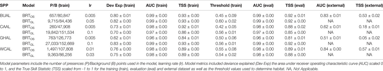
Table 1 Evaluation metrics for Boosted Regression Tree (BRT) models informed by opportunistic sightings data (BRTOS) and geolocation data (BRTGL) for each of the four study species: Buller’s (BUAL), Campbell (CAAL), grey-headed (GHAL), and white-capped (WCAL) albatross.
The ‘gbm.step’ function in the ‘dismo’ package (Hijmans et al., 2020) and evaluation functions in the ‘gbm’ package (Greenwell et al., 2020) were used to fit and evaluate the BRTOS and BRTGL model for each species. Each BRT model was bootstrapped 200 times. For each iteration, a random training dataset consisting of 75% of the presence and background data was drawn and used to fit a BRT model with a Bernoulli error distribution. Following recommendation in Elith et al. (2008) and Leathwick et al. (2006), the learning rate was adjusted for each model type, species/data type, to ensure a minimum tree depth of 1000 was achieved for each bootstrap iteration (see Supplementary Material for additional details).
To assess the importance of each environmental response variable, we calculated the mean relative influence and standard deviation produced by the BRT model across bootstraps. Relative influence is calculated by summing the number of times each variable was chosen for splitting, weighted by the squared improvement of the model as a result of each split. Partial dependence plots were used to visualize model fit across a gradient of values for each environmental variable (Elith et al., 2008). Finally, for each BRT model, the mean monthly predicted probability of occurrence was generated across bootstraps and a final prediction was produced by taking the mean of all monthly predictions.
2.5 Model Evaluation and Predictions
Because RES models do not use presence/availability data to predict probability of occurrence, there are no internal model fit metrics. Therefore, to assess model performance we generated a Receiver Operator Characteristic (ROC) curve by extracting RES model fit values for each presence/availability location used to train species-specific BRTGL models. The threshold value and habitat were then calculated using methods described below for BRT models. The location and area of habitat was compared across models for each species, globally, and within the NZ EEZ.
For BRT models, we assessed model performance by calculating the mean and standard deviation of the deviance explained, the area under the receiver operator characteristic curve (AUC), and the true skill statistic (TSS) from each bootstrap. AUC values range from 0 to 1 with 0 indicating no discrimination, 0.5 no better than random chance, and 1 indicating perfect discrimination ability (Legendre and Legendre, 2012). Models with AUC values ≥ 0.70 are considered ‘useful’ and those with AUC values > 0.9 are considered ‘very good’ because sensitivity is high relative to the false positive rate (Swets, 1988; Pearce and Ferrier, 2000). The TSS scales from -1 to 1 (sensitivity + specificity – 1) and takes into account both omission and commission errors and success as a result of random guessing. Values of 1 are in perfect agreement while values ≤0 indicate performance no better than random or a systematically incorrect prediction (Allouche et al., 2006). TSS values >0.6 are considered useful to excellent (Komac et al., 2016). The AUC is a highly effective measure of the performance and a threshold-independent measure of accuracy, whereas the TSS is a threshold-dependent measure of accuracy that is not sensitive to prevalence (Allouche et al., 2006; Komac et al., 2016).
The performance of BRT models was also assessed using an evaluation dataset consisting of the remaining 25% of the presence/background data not used in the training dataset for each iteration of the bootstrap. Additionally, BRTOS models were further validated using an external dataset consisting of GLS presence/availability data. To create a spatially-explicit measure of uncertainty, we calculated the overall standard deviation for each grid cell by taking the mean of the monthly standard deviations derived from the bootstraps of each model.
To convert predicted probability of occurrence to habitat suitability for each month, we used a model-specific threshold value determined by maximizing the area under the ROC curve (Hijmans et al., 2020). This threshold is the point at which accuracy is the highest and where sensitivity equals specificity. Predicted habitat for each monthly mean probability of occurrence grid was created by classifying cells above the threshold value as 1, and all others as ‘NaN’. Monthly habitat grids were then summed and colour-scaled from 1 to 12, thus reflecting the importance of each cell based on the number of months in which it was classified as habitat. However, because chlorophyll-a data were biased towards the equator and data did not extend as far south in winter compared to summer months, the importance of areas further from the equator may be biased low.
2.6 Overlap With Fishing Effort
Using data downloaded from Global Fishing Watch (GFW) (2020), overlap between the preferred habitat of the four albatross species and fishing effort was examined. Daily global fishing effort data based on vessels fitted with automatic identification system (AIS) transceivers (Kroodsma et al., 2018), were available for five years (2012–2016) at 0.01° resolution. Fishing effort data were not restricted by fishing vessel or gear type. The number of fishing hours that were within the preferred habitat predicted for each species was summed for each month, both globally and within NZ’s EEZ. Mean monthly fishing effort was calculated by averaging replicate months across years. Finally, we quantified the monthly spatial overlap between fishing effort and preferred habitat predicted by each SDM and species. For the top two performing SDMs, mean fishing effort for each month was averaged and bar plots generated using the 'ggplot2' package (Wickham, 2009) in R statistical software to show mean fishing effort for each of the four albatross species, both globally and within NZ’s EEZ.
3 Results
Collinearity between our chosen environmental variables was low (Pearson’s correlation <0.5) and, as such, all variables were retained within our distribution modelling analyses (Supplementary Figures 5–8). Based on model fit measures generated from an evaluation dataset, all BRT models were considered ‘very good’ (AUC (eval) ≥ 0.96, Table 1). Model fit metrics produced from the training and evaluation datasets were similar suggesting limited overfitting to the data and increased transferability of the models to novel datasets. The standard deviations in AUC and TSS performance metrics for all BRT models was ≤0.01 indicating that models performed similarly across all 200 bootstraps. External validation of the BRTOS models using GLS data resulted in lower performance when compared to validation using the evaluation dataset (AUC(external): 0.51-0.84; AUC (eval): 0.96-0.99; Table 1).
AUC values showed that BRT models performed better than RES models (Table 2). AUC values for RES models ranged from 0.57 to 0.88, whereas those for BRT models ranged from 0.96 to 0.99 (Table 2). While most RES models were ‘useful’ (> 0.70), both RES models for CAAL and GHAL were inadequate for distinguishing between presence and availability data and, therefore, not considered useful for predicting probability of occurrence (Table 2). These evaluation metrics showed that models for BUAL performed better than those for other albatross species; results for this species are used as a case study throughout the manuscript. Comparable figures for CAAL, GHAL, and WCAL can be found in the Supplementary Materials.
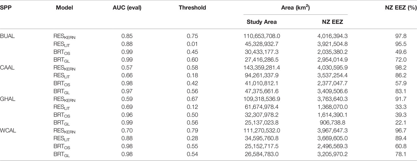
Table 2 The area under the receiver operator characteristic curve (AUC) produced from evaluation data, optimal threshold values for delineating habitat, and area of habitat within the overall study area and the New Zealand Exclusive Economic Zone (EEZ) for four models: two Relative Environmental Suitability models (one fit with values obtained from the monthly 50% kernel density contours from geolocation data (RESKERN), and one fit with values from the literature and expert opinion (RESLIT)) and two Boosted Regression Tree models (one fit with opportunistic sightings data (BRTOS), and one fit with geolocation data (BRTGL)) for four species of albatrosses: Buller’s (BUAL), Campbell (CAAL), grey-headed (GHAL), and white-capped (WCAL).
The environmental niche envelope (area under the trapezoidal response curve) produced from the absolute and preferred values for each variable used to fit RESKERN models was larger than the envelope produced from values used to fit the RESLIT model (Figures 2A–H for BUAL and Supplementary Figures 9A–H, 10A–H, 11A–H for CAAL, GHAL, and WCAL, respectively). The most notable differences between the two RES models were the substantially smaller maximum absolute CHL value used in the RESLIT than the RESKERN model (Figures 2D, H and Supplementary Figures 9D, H, 10D, H, 11D, H).
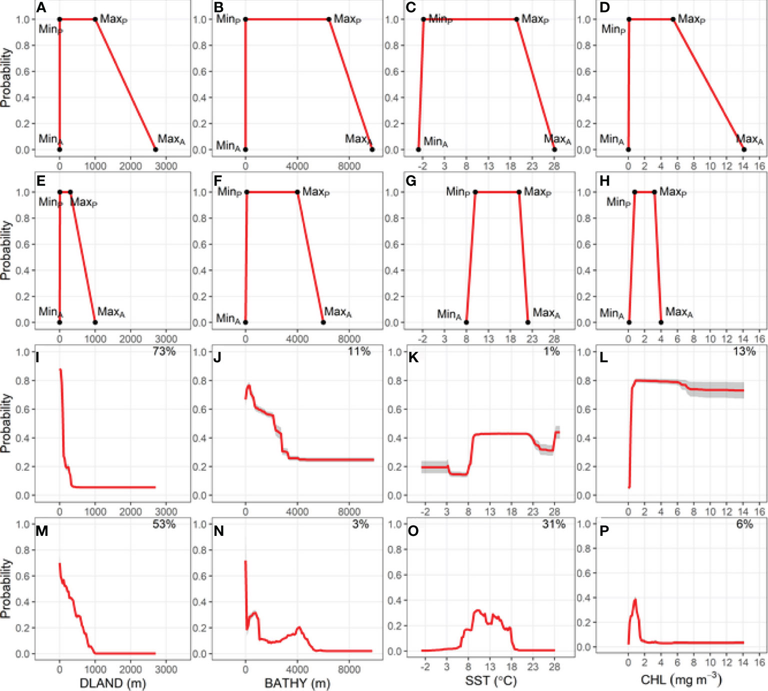
Figure 2 Relationship between the probability of Buller’s albatross occurrence and four environmental variables: Bathymetry (BATHY), distance from land (DLAND), sea surface temperature (SST) and chlorophyll-a (CHL). Top two rows show trapezoidal response curves for each environmental variable used in two Relative Environmental Suitability models (one fit with values obtained from the monthly 50% kernel density contours from geolocation data and background environmental data [RESKERN, (A–D)], and one fit with values from the literature and expert opinion [RESLIT, (E–H)]. Minimum and maximum absolute and preferred habitat values are denoted by MinA, MaxA, MinP, and MaxP. Bottom two rows show partial dependence plots for each environmental variable from two bootstrapped Boosted Regression Tree models (one fit with opportunistic sightings data [BRTOS, (I–L)], and one fit with geolocation data [BRTGL, (M–P)]. Red lines represent response curves with grey shading showing the standard deviation. Percentage contribution for each variable is shown on the top right corner.
Of the four environmental variables, DLAND made the highest or second highest relative contribution to BRTOS models (Figures 2I, L; Supplementary Figures 9I–L, 10I–L, 11I–L). Additionally, BRTOS model results showed that the probability of occurrence was highest closest to land, whereas results from BRTGL models generally revealed more complex relationships (Figures 2I, M and Supplementary Figures 9I, M, 10I, M, 11I, M). With the exception of BUAL, SST had the greatest influence on the probability of occurrence in BRTGL models (Figures 2M–P; Supplementary Figures 9M–P, 10M–P, 11M–P). However, the opposite was true for BRTOS models in which the influence of SST on the probability of occurrence was <15% for all species (Figure 2K and Supplementary Figures 9K, 10K, 11K).
The predicted probability of albatross occurrence varied across the four models, with the RESKERN model predicting the most widespread distribution (Figure 3A and Supplementary Figures 12A, 13A, 14A). Spatially explicit estimates of uncertainty (standard deviations) were higher and more widespread for BRTOS than for BRTGL models (Figure 4 and Supplementary Figures 15-17). In areas outside the minimum convex hull, BRTGL models produced estimates with less uncertainty than BRTOS models.
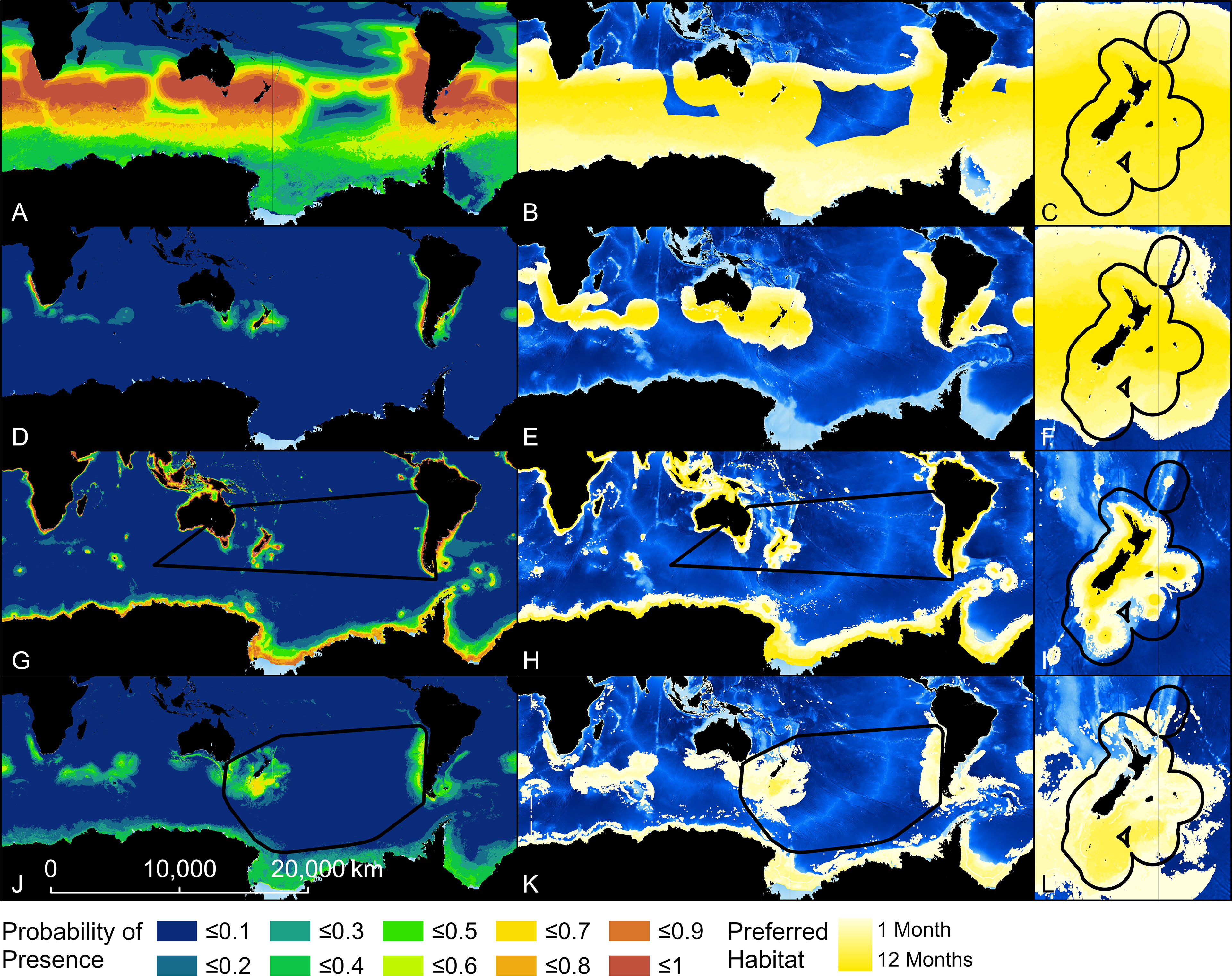
Figure 3 Probability of presence and habitat of Buller’s albatross predicted by four models. Top two rows show results from two Relative Environmental Suitability models [one fit with values obtained from the monthly 50% kernel density contours from geolocation data (RESKERN, A–C)], and one fit with values from the literature and expert opinion [RESLIT, (D–F)]. Bottom two rows show results from two Boosted Regression Tree models (one fit with opportunistic sightings data [BRTOS, (G–I)], and one fit with geolocation data [BRTGL, (J–L)]. Black boundaries indicate the minimum Convex Hull (G, H, J, K) or New Zealand’s Exclusive Economic Zone (C, F, I, L) and habitat is colour-scaled from 1 to 12 indicating the number of months each cell was classified as habitat.
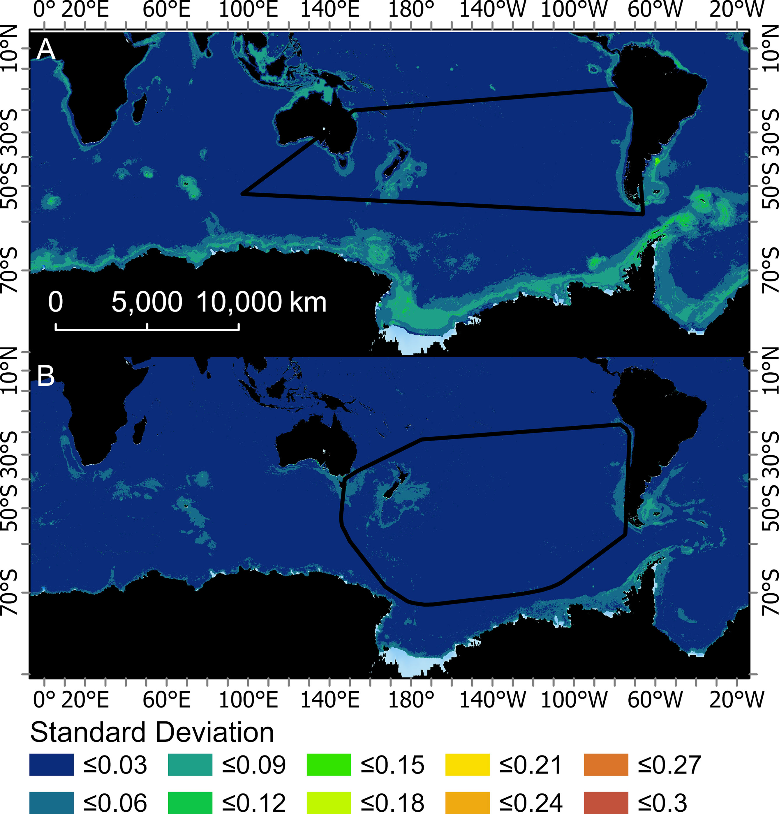
Figure 4 Mean of the monthly standard deviations created from the 200 bootstraps for two boosted regression tree models used to predict the probably of occurrence for Buller’s albatross (one fit with opportunistic sightings data [BRTOS, (A)], and one fit with geolocation data [BRTGL, (B)]. Black boundaries indicate the minimum convex hull around the data that were used to fit each respective BRT model.
Threshold values used to indicate habitat ranged between 0.01 (BUAL RESLIT model) to 0.79 (WCAL RESKERN model) (Table 2). For all species, RESKERN models predicted more habitat than RESLIT models and both types of RES models predicted more habitat than BRT models (Figure 3 and Supplementary Figures 12–14). Compared to BRTGL models, RESKern and RESLIT models resulted in a 3.0-4.3 and 1.3-2.5 fold increase in global habitat, respectively (Table 2). Results from BRTGL models showed that CAAL had the highest percentage (83%) of habitat within NZ's EEZ, followed by WCAL (78%), BUAL (72%), and GHAL (22%) (Table 2, Figure 3 and Supplementary Figures 12–14). For BUAL and GHAL, the percentage of habitat within the overall study area predicted by the BRTOS models was greater than from BRTGL models, while the opposite applied to CAAL and WCAL. Higher probability of occurrence was predicted closer to the coast by BRTOS than by BRTGL models.
Overlap in fishing effort and predicted habitat varied by model, month, and species. For BUAL, CAAL, and GHAL, there was less overlap between fishing effort and preferred habitat predicated by BRTGL models globally across all months than for the other three models (Figure 5 and Supplementary Figures 18–20). For WCAL, global overlap between preferred habitat predicted by the four models was more variable, with predictions from the BRTGL model having higher overlap with fishing effort from March to May than some of the other models (Supplementary Figure 20). Within the EEZ, CAAL and WCAL experienced similar amounts of overlap between monthly fishing effort and preferred habitat across models, particularly from June to August (Supplementary Figures 18 and 20). For GHAL, overlap was the greatest between monthly fishing effort and preferred habitat predicted by RESKERN models, both globally and within NZ’s EEZ (Supplementary Figure 19).
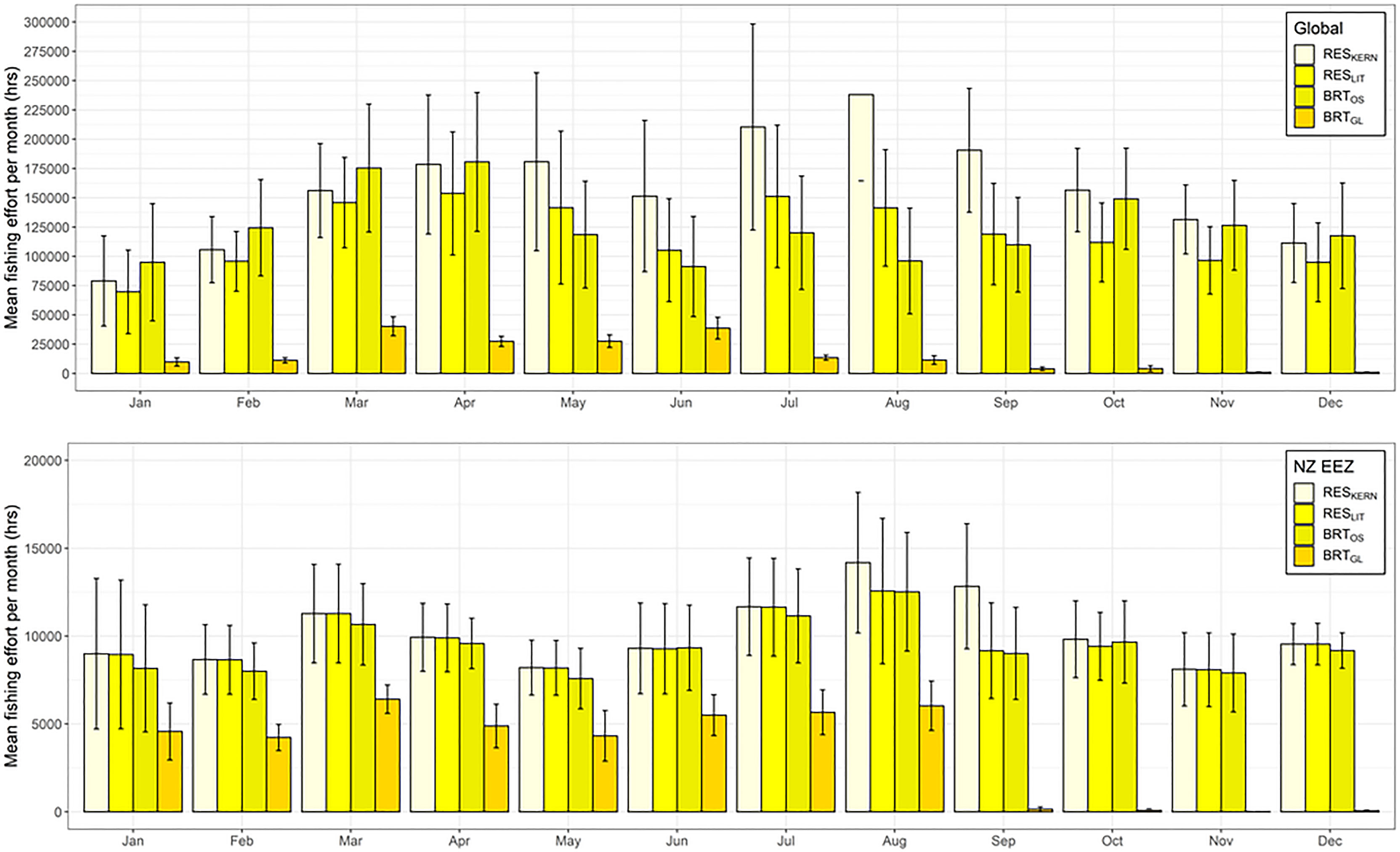
Figure 5 Mean total fishing effort (hrs) (based on data from Global Fishing Watch) per month that occurs within the predicted preferred habitat of Buller’s albatross both globally (top) and within New Zealand’s Exclusive Economic Zone (bottom). Colour coding denotes different habitat suitability models and error bars indicate one standard deviation.
Globally and within NZ's EEZ, BUAL and CAAL experienced the greatest amount of overlap between mean monthly fishing effort and preferred habitat, followed by WCAL (Figure 6). Across both locations and models, GHAL had the least amount of overlap between fishing effort and preferred habitat. The overlap in preferred habitat and fishing effort for WCAL was similar across models. However, for BUAL, CAAL, and GHAL, overlap between fishing effort and preferred habitat predicted by BRTOS models was substantially higher than BRTGL models both globally and within NZ's EEEZ (Figure 6).
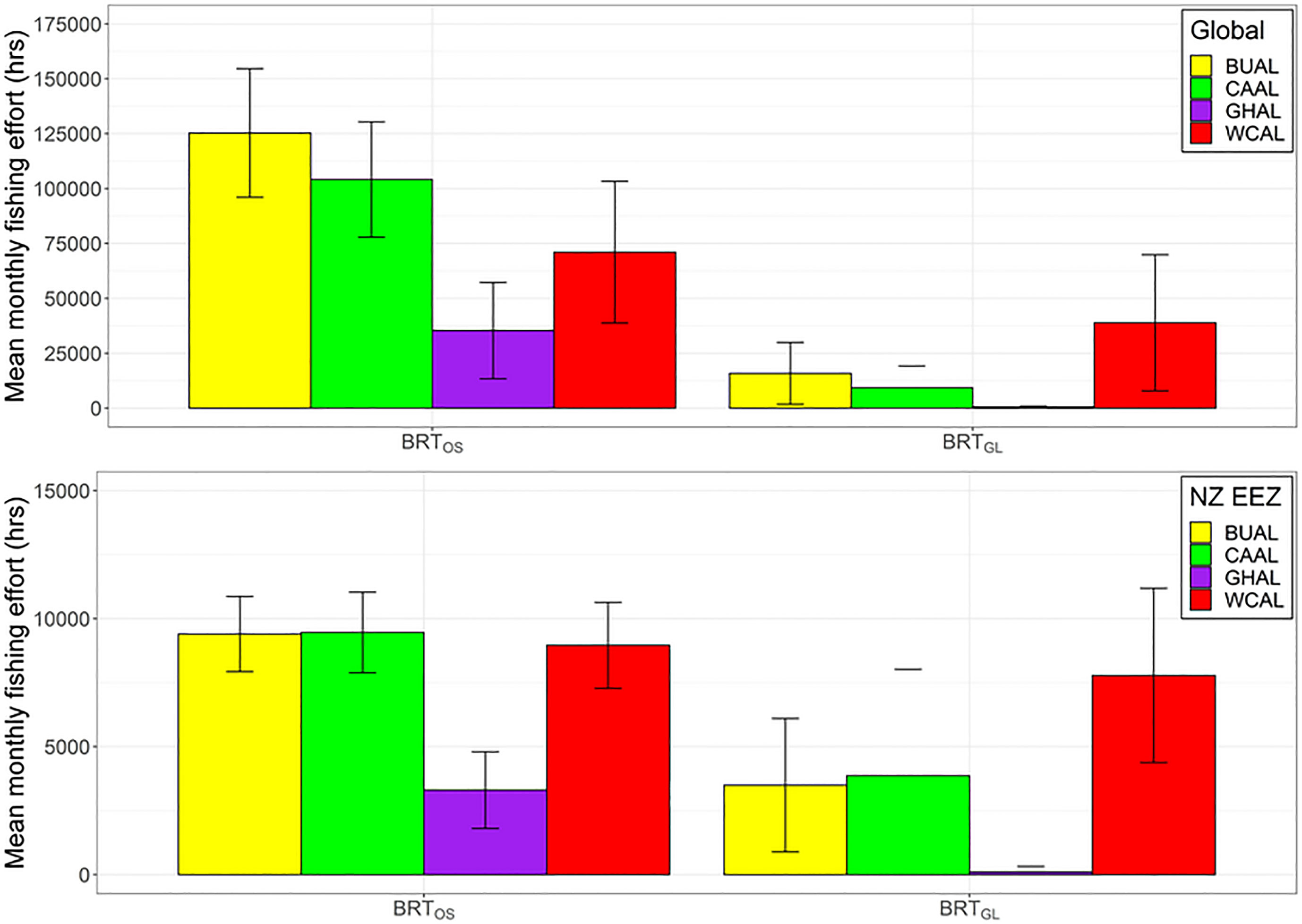
Figure 6 Mean monthly fishing effort (hrs) (based on data from Global Fishing Watch) that occurs within the preferred habitat of four albatross species both globally (top) and within New Zealand’s Exclusive Economic Zone (bottom) for two BRT models (one fit with opportunistic sightings data [BRTOS, left], and one fit with geolocation data [BRTGL, right]. Colour coding denotes different albatross species and error bars indicate one standard deviation.
Discussion
This study is one of a growing body of work that compares results of different SDMs and/or assesses model sensitivity to differences in sample size or model parameters (Peterson and Cohoon, 1999; Stockwell and Peterson, 2002; Loiselle et al., 2003; Johnson and Gillingham, 2005; Lütolf et al., 2006; Johnson and Gillingham, 2008; Mouton et al., 2010; Porfirio et al., 2014). Here we show that, while keeping environmental variables and modelling techniques as comparable as possible, incremental increases in data quality resulted in increased resolution of SDM predictions, adding value and confidence in derived species conservation efforts. In our study, BRT models for all four species of albatross outperformed RES models and predictions were in agreement with what is generally known about the species. BRT models offer a predictive advantage over RES models by being able to identify relevant variables and the capability of incorporating environmental interactions. Additionally, BRT models provided explicit estimates of model uncertainty (as seen by the bootstrapping method employed in this study).
Evaluation metrics produced from the training and evaluation datasets showed that both BRT models performed well (AUC > 96; TSS > 0.81). However, evaluation metrics from an external dataset consisting of GLS data were greatly reduced (AUC: 51-84; TSS: 0.05-0.57; Table 2), suggesting that BRTOS models are overly optimistic and may not be able to predict probability of occurrence and habitat suitably as accurately as BRTGL models. While the partial dependency plots for BRTGL models revealed a complex relationship between species occurrence and environmental variables, partial dependence plots for BRTOS models for each species showed a distinct preference for shallow areas close to land which is likely the result of the sighting locations rather than a reflection of true habitat preference. This finding is most certainly due to the notoriously biased nature of opportunistic sightings towards coastal areas with higher human populations which greatly under-represents the use of remote, at-sea areas important to albatrosses. Opportunistic sightings also lack a behavioural component, unlike GLS or other high resolution data from which it is often possible to differentiate between behaviors such as flying, resting, and feeding. For examples, the kernels produced in this study are greatly influenced by where animals spend the most time, most likely to be an indication of foraging as opposed to transiting.
However, in the absence of empirical data, RES models offer a standardized, quantitative approach for investigating the distribution of wide-ranging species (Kaschner et al., 2006; Watson et al., 2013) and offer more objectivity than hand drawn distribution maps (Kaschner et al., 2006). For all four albatross species, RES models resulted in at least double the area of habitat within the study region than BRT models fit with seabird GLS data. This finding is most likely due the oversimplified trapezoidal response curve which is inadequate for capturing the complex relationship between species' occurrence and environmental conditions. Additionally, RES models assume that all variables are equally weighted in predicting species distribution, which is rarely true (e.g. as shown in the results of both BRT models presented here). Furthermore, due to information gaps that exist for many species, RES models are likely to underrepresent offshore areas that are less frequently observed. For these reasons, RES models should not be used as an alternative to empirical data which is able to more accurately predict species occurrence.
When comparing RES models, differences between RESKERN and RESLIT model predictions are due to the wider range of environmental values for used to fit RESKERN models. These ranges were based on values from the year-round GLS data which may include a wider range of values than those found in the literature as studies are more likely to focus on a particular life stage (e.g. incubation or chick-rearing). RES models based on literature and expert opinion performed markedly better than the RES model with wider environmental ranges. The lower threshold for the RESLIT models indicates a higher sensitivity or true positive rate. However, neither of the two RES models for CAAL and GHAL were able to adequately distinguish between presences and background data (AUC ≤ 0.7), and, therefore, were not considered useful for predicting probability of occurrence or habitat. Thus, care must be taken when relying on less data-rich models.
Understanding potential biases in the data is important as it may lead to incorrect conclusions about species' habitat preference as well as the inability to identify population-level differences in habitat use patterns. Different populations of the same species can have different relationships to their environment (Torres et al., 2015). While this is not an issue for BUAL, CAAL, and WCAL that are endemic to an island group or small region within NZ waters, using sightings data for species that occupy multiple wide-spread colonies such as GHAL can result in incorrect relationships between species’ occurrence and the environment. Further complicating the use of opportunistic sighting records is the difficulty in distinguishing between morphologically similar species such as CAAL/black-browed (Thalassarche melanophris) albatrosses, WCAL/shy (Thalassarche cauta) albatrosses and between sub-species such as southern and northern BUAL. For example, the southern sub-species of BUAL breeds only at the Snares and Solander Islands whereas the northern sub-species breeds three months earlier, mostly at the Chatham Islands (Stahl et al., 1998). The misidentification of species or sub-species is likely to result in inadequate or inaccurate predicted probability of occurrence and habitat over both space and time.
When developing SDMs to predict occurrence, care must be taken to collect data at the same spatial and temporal scale as its intended conservation or management use. Species’ movement and distribution may vary between breeding and non-breeding seasons (as is the case for many species of seabirds), thus distribution maps developed from data collected during the breeding season should not be used to extrapolate to the non-breeding season. SDMs built from data covering only a portion of a species’ range may provide poor predictions on range-wide needs if data are extrapolated (Peterson and Cohoon, 1999). For comparison purposes, our study compared preferred habitat both globally and within NZ’s EEZ for all species. However, preferred habitat predicted beyond the extent of the underlying data for both opportunistic sighing and GLS datasets should be interpreted with care. For example, BRT models frequently predicted preferred habitat in the Ross Sea, near Antarctica, where albatrosses are very unlikely to visit.
One example of how data quality can influence conservation and management is our ability to assess risk from fishing effort. Historically, in the absence of high-quality data on seabird movement and foraging behaviour, estimates of distribution ranges have consisted of hand-drawn maps outlining the proposed maximum extent of species' occurrence according to expert opinion (e.g. S. Ridgway and Harrison (1981), S. H. Ridgway (1985), and S. H. Ridgway and Harrison (1989)). Currently, tracking data are often used to estimate seabird-fisheries overlap (Suryan et al., 2007; Votier et al., 2010; Torres et al., 2011; Torres et al., 2013; Sztukowski et al., 2017; Clay et al., 2019). BTR models fit with relatively high-resolution GLS data offer greater refinement of predicted habitat than distribution maps included in NZ’s National Aquatic Biodiversity Information System (NABIS, www.nabis.govt.nz) which, in the absence of other data, are sometimes hand-drawn and used to examine the overlap between seabird species occurrence and commercial fisheries (Richard et al., 2017; Richard et al., 2020). Additionally, distribution maps used to calculate risk of seabird bycatch by NZ commercial fisheries are typically computed as annual averages and do not account for seasonal changes in distribution that would occur during migration or at different stages of the breeding cycle (Richard et al., 2017).
Our study showed that there are substantial differences in the overlap between fishing effort and preferred habitat across species. RESKERN models based on little to no empirical data predicted the most preferred habitat which subsequently overlapped with the most fishing effort, globally, compared to the preferred habitat predicted by BRT models informed with opportunistic sighting or geolocation data. Even though BRTOS models predicted either the smallest or next to the smallest area of preferred habitat, overlap with fishing effort was often higher than for the RESLIT and BRTGL models. This is likely due to bias from coastal sightings data that, in turn, biases model predictions towards coastal regions. This pattern tended to occur during from October to April for BUAL and WCAL, from September to March for CAAL, and nearly year-round for GHAL. For WCAL and CAAL, these times correspond to the breeding period where birds were constrained to regions near colonies where fishing occurs. While this timing does not correspond to the breeding period for BUAL, preferred habitat predicted by the BRTOS model was located exclusively in coastal habitats or within NZ’s EEZ where fishing is likely to be highest. For the two best performing models (BRTOS and BRTGL), the greatest overlap between predicted preferred habitat and fishing effort across all months occurred for BUAL and CAAL, both globally and within NZ’s EEZ, while GHAL had the least amount of overlap, likely due to this species’ preference for pelagic waters beyond NZ’s EEZ where fishing effort is typically reduced. Additionally, overlap between mean monthly fishing effort and preferred habitat predicted by BRTOS models was higher than for BRTGL models for all species. Again, this finding is likely due to a coastal bias in opportunistic sighting data, resulting in SDMs that are unable to adequately predict to offshore areas where birds are known to occur. Although trends in overlap between fishing effort and preferred habitat between species and models may be accurate, it is important to keep in mind that the total number of fishing effort hours shown in this study are only an indication on minimum effort because GFW data represents only 50-75% of active vessels that are > 24 m in length that were fitted with AIS transceivers (Kroodsma et al., 2018; Shepperson et al., 2018).
Currently, BUAL, CAAL, and WCAL are considered vulnerable to capture by NZ commercial fisheries, and across the different risk categories, albatross species comprise half of the ‘very high’ or ‘high’ risk categories (Richard et al., 2020). Both BRT models showed that WCAL, BUAL, and CAAL have the highest overlap with fishing effort. These species also have some of the highest number of capture by NZ commercial fisheries recorded by government observers (963, 681, and 46, respectively), between the fishing years 2006-07 and 2016-17 (Richard et al., 2020). These albatross species are categorized as ‘high risk’ (BUAL), ‘medium risk’ (WCAL), and ‘low risk’ (CAAL) of capture (GHAL is categorized as ‘negligible risk’), which is largely driven by calculated overlap with fishing effort (Richard et al., 2020). In our study, preferred habitat of CAAL within NZ’s EEZ predicted by BRTOS and BRTGL models had the highest and second highest overlap with fishing effort, respectively, suggesting that commercial fisheries may pose a greater risk to CAAL than currently recognised. Additionally, the overlap of preferred habitat predicted by the best performing model (BRTGL) with fishing effort was highest from June to August, further supporting the findings of Thompson et al. (2021) which determined that the risk of NZ fisheries to CAAL was greatest in the non-breeding season.
Because miscalculations in the overlap between seabird distribution and fishing effort can lead to ineffective mitigation measure to reduce seabird bycatch in commercial fisheries, resource managers will most certainly benefit in the collection of higher quality data. This study showed that higher quality data resulted in more refined areas of predicted habitat than NABIS maps used by NZ management agencies. Additionally, the predicted habitat from models that used higher quality data usually resulted in less overlap with fishing efforts. Therefore, investing in the collection of collecting high-quality seabird data may ultimately lead to cost savings and more targeted management solutions in the long run. One must carefully balance the trade-offs of (1) investing resources up front to collect robust long-term biologging data resulting in more accurate, targeted, areas of potential protection, and (2) using existing low-resolution or no data for relatively little cost resulting in larger, less-accurate, predicted habitat that will require substantial resources to protect and is less likely to provide conservation benefit. While using existing data saves money in the short-term, the collection of high-quality long-term data can provide distribution information at various spatial-temporal scales that are more likely to lead to effective future management decisions and the ability to better assess potential threats from commercial fisheries.
Data Availability Statement
The datasets presented in this study can be found in online repositories. The names of the repository/repositories and accession number(s) can be found below: BirdLife’s Seabird Tracking Database (see http://www.seabirdtracking.org/).
Ethics Statement
Methods used to obtain tracking data from live animals were reviewed and approved by NIWA's Animal Ethics Committee.
Author Contributions
DT and KG conceived the idea. RO, PS, LT, LS, CK, RP, SV, SB, GT, and DT collected the data. KG, RO, and DT collated the data. KG, FS, AH, and AB analysed the data. KG and DT led the writing. All authors contributed to the article and approved the submitted version.
Funding
This work was funded by the Innovation Fund of the Sustainable Seas National Science Challenge, the New Zealand Ministry for Business, Innovation and Employment, the New Zealand Department of Conservation, and by the National Institute of Water and Atmospheric Research Ltd.
Conflict of Interest
The authors declare that the research was conducted in the absence of any commercial or financial relationships that could be construed as a potential conflict of interest.
The handling Editor declared a past co-authorship with several of the authors KG, LT, RP, and DRT.
Publisher’s Note
All claims expressed in this article are solely those of the authors and do not necessarily represent those of their affiliated organizations, or those of the publisher, the editors and the reviewers. Any product that may be evaluated in this article, or claim that may be made by its manufacturer, is not guaranteed or endorsed by the publisher.
Acknowledgments
Many thanks to Josh London and Elliott Hazen for the support and analysis guidance and to the many people involved in the logistics that resulted in the data used in this study. The findings and conclusions in this paper are those of the author(s) and do not necessarily represent the views of the National Marine Fisheries. Service, NOAA. Mention of trade names and commercial firms does not imply endorsement by the National Marine Fisheries Service, NOAA.
Supplementary Material
The Supplementary Material for this article can be found online at: https://www.frontiersin.org/articles/10.3389/fmars.2022.782923/full#supplementary-material
References
Allouche O., Tsoar A., Kadmon R. (2006). Assessing the Accuracy of Species Distribution Models: Prevalence, Kappa and the True Skill Statistic (TSS). J. Appl. Ecol. 43, 1223–1232. doi: 10.1111/j.1365-2664.2006.01214.x
Anderson O. R., Small C. J., Croxall J. P., Dunn E. K., Sullivan B. J., Yates O., et al. (2011). Global Seabird Bycatch in Longline Fisheries. Endanger. Species Res. 14, 91–106. doi: 10.3354/esr00347
Augé A. A., Dias M. P., Lascelles B., Baylis A. M., Black A., Boersma P. D., et al. (2018). Framework for Mapping Key Areas for Marine Megafauna to Inform Marine Spatial Planning: The Falkland Islands Case Study. Mari. Policy 92, 61–72. doi: 10.1016/j.marpol.2018.02.017
Benito B. M., Martínez-Ortega M. M., Munoz L. M., Lorite J., Penas J., Conservation (2009). Assessing Extinction-Risk of Endangered Plants Using Species Distribution Models: A Case Study of Habitat Depletion Caused by the Spread of Greenhouses. Biodiversity 18, 2509–2520. doi: 10.1007/s10531-009-9604-8
Bindoff A. D., Wotherspoon S. J., Guinet C., Hindell M. A. (2018). Twilight-Free Geolocation From Noisy Light Data. Methods Ecol. Evol. 9, 1190–1198. doi: 10.1111/2041-210X.12953
Block B. A. (2005). Physiological Ecology in the 21st Century: Advancements in Biologging Science1. Integr. Comp. Biol. 45, 305–320. doi: 10.1093/icb/45.2.305
Bluhm B. A., Coyle K. O., Konar B., Highsmith R. (2007). High Gray Whale Relative Abundances Associated With an Oceanographic Front in the South-Central Chukchi Sea. Deep-Sea Res. Part II Topical Stud. Oceanogr. 54, 2919–2933. doi: 10.1016/j.dsr2.2007.08.015
Calenge C. (2006). The Package “Adehabitat” for the R Software: A Tool for the Analysis of Space and Habitat Use by Animals. Ecol. Modelling 197, 516–519. doi: 10.1016/j.ecolmodel.2006.03.017
Clay T. A., Manica A., Ryan P. G., Silk J. R., Croxall J. P., Ireland L., et al. (2016). Proximate Drivers of Spatial Segregation in Non-Breeding Albatrosses. Sci. Rep. 6, 29932. doi: 10.1038/srep29932
Clay T. A., Small C., Tuck G. N., Pardo D., Carneiro A. P., Wood A. G., et al. (2019). A Comprehensive Large-Scale Assessment of Fisheries Bycatch Risk to Threatened Seabird Populations. J. Appl. Ecol. 56, 1882–1893. doi: 10.1111/1365-2664.13407
Cooke S. J. (2008). Biotelemetry and Biologging in Endangered Species Research and Animal Conservation: Relevance to Regional, National, and IUCN Red List Threat Assessments. Endanger. Species Res. 4, 165–185. doi: 10.3354/esr00063
Croxall J. P., Butchart S. H., Lascelles B., Stattersfield A. J., Sullivan B., Symes A., et al. (2012). Seabird Conservation Status, Threats and Priority Actions: A Global Assessment. Bird Conserv. Int. 22, 1–34. doi: 10.1017/S0959270912000020
Derville S., Torres L. G., Iovan C., Garrigue C. (2018). Finding the Right Fit: Comparative Cetacean Distribution Models Using Multiple Data Sources and Statistical Approaches. Divers. Distrib. 24, 1657–1673. doi: 10.1111/ddi.12782
Dias M. P., Oppel S., Bond A. L., Carneiro A. P., Cuthbert R. J., González-Solís J., et al. (2017). Using Globally Threatened Pelagic Birds to Identify Priority Sites for Marine Conservation in the South Atlantic Ocean. Biol. Conserv. 211, 76–84. doi: 10.1016/j.biocon.2017.05.009
ebird (2021). eBird: An Online Database of Bird Distribution and Abundance [Web Application]. eBird (Cornell Lab of Ornithology, Ithaca, New York). Available at: http://www.ebird.org. (Accessed February 2, 2021)
Elith J., Kearney M., Phillips S. (2010). The Art of Modelling Range-Shifting Species. Methods Ecol. Evol. 1, 330–342. doi: 10.1111/j.2041-210X.2010.00036.x
Elith J., Leathwick J. R. (2009). Species Distribution Models: Ecological Explanation and Prediction Across Space and Time. Annu. Rev. Ecol. Evol. Syst. 40, 677–697. doi: 10.1146/annurev.ecolsys.110308.120159
Elith J., Leathwick J. R., Hastie T. (2008). A Working Guide to Boosted Regression Trees. J. Anim. Ecol. 77, 802–813. doi: 10.1111/j.1365-2656.2008.01390.x
Etnoyer P., Canny D., Mate B. R., Morgan L. E., Ortega-Ortiz J. G., Nichols W. J. (2006). Sea-Surface Temperature Gradients Across Blue Whale and Sea Turtle Foraging Trajectories Off the Baja California Peninsula, Mexico. Deep-Sea Res. Part II Topical Stud. Oceanogr. 53, 340–358. doi: 10.1016/j.dsr2.2006.01.010
Evans K., Lea M. A., Patterson T. A. (2013). Recent Advances in Bio-Logging Science: Technologies and Methods for Understanding Animal Behaviour and Physiology and Their Environments. Deep Sea Res. Part II: Topical Stud. Oceanogr. 88-89, 1–6. doi: 10.1016/j.dsr2.2012.10.005
Franklin J. (2010). Moving Beyond Static Species Distribution Models in Support of Conservation Biogeography. Divers. Distrib. 16, 321–330. doi: 10.1111/j.1472-4642.2010.00641.x
Friendly M. (2002). Corrgrams: Exploratory Displays for Correlation Matrices. Am. Stat. 56, 316–324. doi: 10.1198/000313002533
Fuentes-Castillo T., Scherson R. A., Marquet P. A., Fajardo J., Corcoran D., Román M. J., et al. (2019). Modelling the Current and Future Biodiversity Distribution in the Chilean Mediterranean Hotspot. The Role of Protected Areas Network in a Warmer Future. Divers. Distrib. 25, 1897–1909. doi: 10.1111/ddi.12988
Gerrodette T., Eguchi T. (2011). Precautionary Design of a Marine Protected Area Based on a Habitat Model. Endanger. Species Res. 15, 159–166. doi: 10.3354/esr00369
Goetz K., Montgomery R., Ver Hoef J., Hobbs R. (2012). Identifying Esssential Habitat of the Endangered Belgua Whale in Cook Inlet, Alaska. Endanger. Species Res. 16, 135–147. doi: 10.3354/esr00394
Greenwell B., Boehmke B., Cunningham J., Gbm Developers. (2020). Gbm: Generalized Boosted Regression Models. Available at: https://CRAN.R-project.org/package=gbm.
Guisan A., Zimmermann N. E. (2000). Predictive Habitat Distribution Models in Ecology. Ecol. Model. 135, 147–186. doi: 10.1016/S0304-3800(00)00354-9
Hays G. C., Bailey H., Bograd S. J., Bowen W. D., Campagna C., Carmichael R. H., et al. (2019). Translating Marine Animal Tracking Data Into Conservation Policy and Management. Trends Ecol. Evol. 34, 459–473. doi: 10.1016/j.tree.2019.01.009
Hijmans R. J. (2020). Raster: Geographic Data Analysis and Modeling. Available at: https://CRAN.R-project.org/package=raster.
Hijmans R. J., Phillips S., Leathwick J., Elith J. (2020) Dismo: Species Distribution Modeling. Available at: https://CRAN.R-project.org/package=dismo.
Hindell M. A., Reisinger R. R., Ropert-Coudert Y., Hückstädt L. A., Trathan P. N., Bornemann H., et al. (2020). Tracking of Marine Predators to Protect Southern Ocean Ecosystems. Nature 580, 87–92. doi: 10.1038/s41586-020-2126-y
Hooker S. K., Whitehead H., Gowans S. (1999). Marine Protected Area Design and the Spatial and Temporal Distribution of Cetaceans in a Submarine Canyon. Conserv. Biol. 13, 592–602. doi: 10.1046/j.1523-1739.1999.98099.x
Hyrenbach K. D., Fernández P., Anderson D. J. (2002). Oceanographic Habitats of Two Sympatric North Pacific Albatrosses During the Breeding Season. Mar. Ecol. Prog. Ser. 233, 283–301. doi: 10.3354/meps233283
IUCN (International Union for the Concervation of Nature. (2021). The IUCN Red List of Threatened Species. Available at: https://www.iucnredlist.org.
Jiménez S., Phillips R. A., Brazeiro A., Defeo O., Domingo A. (2014). Bycatch of Great Albatrosses in Pelagic Longline Fisheries in the Southwest Atlantic: Contributing Factors and Implications for Management. Biol. Conserv. 171, 9–20. doi: 10.1016/j.biocon.2013.12.035
Johnson C. J., Gillingham M. P. (2005). An Evaluation of Mapped Species Distribution Models Used for Conservation Planning. Environ. Conserv. 32, 117–128. doi: 10.1017/S0376892905002171
Johnson C. J., Gillingham M. P. (2008). Sensitivity of Species-Distribution Models to Error, Bias, and Model Design: An Application to Resource Selection Functions for Woodland Caribou. Ecol. Model. 213, 143–155. doi: 10.1016/j.ecolmodel.2007.11.013
Kaschner K., Tittensor D. P., Ready J., Gerrodette T., Worm B. (2011). Current and Future Patterns of Global Marine Mammal Biodiversity. PloS One 6, e19653. doi: 10.1371/journal.pone.0019653
Kaschner K., Watson R., Trites A., Pauly D. (2006). Mapping World-Wide Distributions of Marine Mammal Species Using a Relative Environmental Suitability (RES) Model. Mar. Ecol. Prog. Ser. 316, 285–310. doi: 10.3354/meps316285
Komac B., Esteban P., Trapero L., Caritg R. (2016). Modelization of the Current and Future Habitat Suitability of Rhododendron Ferrugineum Using Potential Snow Accumulation. PloS One 11, e0147324. doi: 10.1371/journal.pone.0147324
Kroodsma D. A., Mayorga J., Hochberg T., Miller N. A., Boerder K., Ferretti F., et al. (2018). Tracking the Global Footprint of Fisheries. Science 359, 904–908. doi: 10.1126/science.aao5646
Laidre K. L., Stirling I., Lowry L. F., Wiig Ø., Heide-Jørgensen M. P., Ferguson S. H. (2008). Quantifying the Sensitivity of Arctic Marine Mammals to Climate-Induced Habitat Change. Ecol. Appl. 18, S97–S125. doi: 10.1890/06-0546.1
Leathwick J., Elith J., Francis M., Hastie T., Taylor P. (2006). Variation in Demersal Fish Species Richness in the Oceans Surrounding New Zealand: An Analysis Using Boosted Regression Trees. Mar. Ecol. Prog. Ser. 321, 267–281. doi: 10.3354/meps321267
Lewison R. L., Crowder L. B. (2003). Estimating Fishery Bycatch and Effects on a Vulnerable Seabird Population. Ecol. Appl. 13, 743–753. doi: 10.1890/1051-0761(2003)013[0743:EFBAEO]2.0.CO;2
Loiselle B. A., Howell C. A., Graham C. H., Goerck J. M., Brooks T., Smith K. G., et al. (2003). Avoiding Pitfalls of Using Species Distribution Models in Conservation Planning. Conserv. Biol. 17, 1591–1600. doi: 10.1111/j.1523-1739.2003.00233.x
Louzao M., Hyrenbach K. D., Arcos J. M., Abelló P., De Sola L. G., Oro D. (2006). Oceanographic Habitat of an Endangered Mediterranean Procellariiform: Implications for Marine Protected Areas. Ecol. Appl. 16, 1683–1695. doi: 10.1890/1051-0761(2006)016[1683:OHOAEM]2.0.CO;2
Lütolf M., Kienast F., Guisan A. (2006). The Ghost of Past Species Occurrence: Improving Species Distribution Models for Presence-Only Data. J. Appl. Ecol. 43, 802–815. doi: 10.1111/j.1365-2664.2006.01191.x
Moilanen A., Franco A. M., Early R. I., Fox R., Wintle B., Thomas C. D. (2005). Prioritizing Multiple-Use Landscapes for Conservation: Methods for Large Multi-Species Planning Problems. Proc. R. Soc. B: Biol. Sci. 272, 1885–1891. doi: /10.1098/rspb.2005.3164
Mouton A. M., De Baets B., Goethals P. L. (2010). Ecological Relevance of Performance Criteria for Species Distribution Models. Ecol. Model. 221, 1995–2002. doi: 10.1016/j.ecolmodel.2010.04.017
Murdoch D., Chow E. (1996). A Graphical Display of Large Correlation Matrices. Am. Stat. 50, 178–180. doi: 10.1080/00031305.1996.10474371
Oliveira U., Soares-Filho B. S., Paglia A. P., Brescovit A. D., De Carvalho C. J., Silva D. P., et al. (2017). Biodiversity Conservation Gaps in the Brazilian Protected Areas. Sci. Rep. 7, 1–9. doi: 10.1038/s41598-017-08707-2
Pearce J., Ferrier S. (2000). An Evaluation of Alternative Algorithms for Fitting Species Distribution Models Using Logistic Regression. Ecol. Model. 128, 127–147. doi: 10.1016/S0304-3800(99)00227-6
Peterson A. T., Cohoon K. P. (1999). Sensitivity of Distributional Prediction Algorithms to Geographic Data Completeness. Ecol. Modelling 117, 159–164. doi: 10.1016/S0304-3800(99)00023-X
Phillips R., Silk J., Croxall J., Afanasyev V., Briggs D. (2004). Accuracy of Geolocation Estimates for Flying Seabirds. Mar. Ecol. Prog. Ser. 266, 265–272. doi: 10.3354/meps266265
Pliscoff P., Luebert F., Hilger H. H., Guisan A. (2014). Effects of Alternative Sets of Climatic Predictors on Species Distribution Models and Associated Estimates of Extinction Risk: A Test With Plants in an Arid Environment. Ecol. Model. 288, 166–177. doi: 10.1016/j.ecolmodel.2014.06.003
Porfirio L. L., Harris R. M., Lefroy E. C., Hugh S., Gould S. F., Lee G., et al. (2014). Improving the Use of Species Distribution Models in Conservation Planning and Management Under Climate Change. PloS One 9, e113749. doi: 10.1371/journal.pone.0113749
Ramírez I., Paiva V. H., Menezes D., Silva I., Phillips R. A., Ramos J. A., et al. (2013). Year-Round Distribution and Habitat Preferences of the Bugio Petrel. Mari. Ecol. Prog. Ser. 476, 269–284. doi: 10.3354/meps10083
R Core Team (2020). R: A Language and Environment for Statistical Computing. R Foundation for Statistical Computing (Vienna, Austria). Available at: https://www.R-project.org/.
Richard Y., Abraham E., Berkenbusch K. (2017). Assessment of the Risk of Commercial Fisheries to New Zealand Seabird–07 to 2014–15. N. Z. Aquat. Environ. Biodiversity Rep. 191, 104.
Richard Y., Abraham E., Berkenbusch K. (2020). Assessment of the Risk of Commercial Fisheries to New Zealand Seabird–07 to 2016–17. N. Z. Aquat. Environ. Biodiversity Rep. 237, 57.
Ridgway S. H., Harrison R. J. (1989). River Dolphins and the Larger Toothed Whales (London, New York: Academic Press).
Robertson H., Baird K., Dowding J., Elliott G., Hitchmough R., Miskelly C., et al. (2017). Conservation Status of New Zealand Birds, 2016. New Zealand Threat Classifcation Series 19.
Rodríguez J. P., Brotons L., Bustamante J., Seoane J. J. D. (2007). The Application of Predictive Modelling of Species Distribution to Biodiversity Conservation. Divers. Distrib. 13, 243–251. doi: 10.1111/j.1472-4642.2007.00356.x
Rowden A., Stephenson F., Clark M., Anderson O., Guinotte J., Baird S., et al. (2019). Examining the Utility of a Decision-Support Tool to Develop Spatial Management Options for the Protection of Vulnerable Marine Ecosystems on the High Seas Around New Zealand. Ocean Coastal Manage. 170, 1–16. doi: 10.1016/j.ocecoaman.2018.12.033
Sharp B. R. (2017). "Spatially Explicit Fisheries Risk Assessment (SEFRA): A Framework for Quantifying and Managing Incidental Commercial Fisheries Impacts on Non-Target Species and Habitats", in Aquatic Environment and Biodiversity Annual Review 2016 (Wellington: Fisheries Management Science Team, Ministry for Primary Industries).
Shepperson J. L., Hintzen N. T., Szostek C. L., Bell E., Murray L. G., Kaiser M. J. (2018). A Comparison of VMS and AIS Data: The Effect of Data Coverage and Vessel Position Recording Frequency on Estimates of Fishing Footprints. ICES J. Mari. Sci. 75, 988–998. doi: 10.1093/icesjms/fsx230
Stahl J., Bartle J., Cheshire N., Petyt C., Sagar P. (1998). Distribution and Movements of Buller's Albatross (Diomedea Bulleri) in Australasian Seas. N. Z. J. Zool. 25, 109–137. doi: 10.1080/03014223.1998.9518143
Stephenson F., Goetz K., Sharp B., Mouton T., Beets F., Roberts J., et al. (2020). Modelling the Spatial Distribution of Cetaceans in New Zealand Waters. Divers. Distrib. 26, 495–516. doi: 10.1111/ddi.13035
Stockwell D. R., Peterson A. T. (2002). Effects of Sample Size on Accuracy of Species Distribution Models. Ecol. Model. 148, 1–13. doi: 10.1016/S0304-3800(01)00388-X
Suryan R. M., Dietrich K. S., Melvin E. F., Balogh G. R., Sato F., Ozaki K. (2007). Migratory Routes of Short-Tailed Albatrosses: Use of Exclusive Economic Zones of North Pacific Rim Countries and Spatial Overlap With Commercial Fisheries in Alaska. Biol. Conserv. 137, 450–460. doi: 10.1016/j.biocon.2007.03.015
Swets J. A. (1988). Measuring the Accuracy of Diagnostic Systems. Science 240, 1285–1293. doi: 10.1126/science.3287615
Sztukowski L. A., Van Toor M. L., Weimerskirch H., Thompson D. R., Torres L. G., Sagar P. M., et al. (2017). Tracking Reveals Limited Interactions Between Campbell Albatross and Fisheries During the Breeding Season. J. Ornithol. 158, 725–735. doi: 10.1007/s10336-016-1425-4
Tancell C., Sutherland W. J., Phillips R. (2016). Marine Spatial Planning for the Conservation of Albatrosses and Large Petrels Breeding at South Georgia. Biol. Conserv. 198, 165–176. doi: 10.1016/j.biocon.2016.03.020
Thompson D., Goetz K., Sagar P., Torres L., Kroeger C., Sztukowski L., et al. (2021). The Year-Round Distribution of Campbell Albatross (Thalassarche Impavida). Aquat. Conserv,: Mar. Freshw. Ecosyst. 31(10):1–12. doi: 10.1002/aqc.3685
Torres L., Read A., Halpin P. (2008). Fine-Scale Habitat Modeling of a Top Marine Predator: Do Prey Data Improve Predictive Capacity? Ecol. Appl. 18, 1702–1717. doi: 10.1890/07-1455.1
Torres L. G., Sagar P. M., Thompson D. R., Phillips R. (2013). Scaling Down the Analysis of Seabird-Fishery Interactions. Mar. Ecol. Prog. Ser. 473, 275–289. doi: 10.3354/meps10071
Torres L. G., Sutton P. J., Thompson D. R., Delord K., Weimerskirch H., Sagar P. M., et al. (2015). Poor Transferability of Species Distribution Models for a Pelagic Predator, the Grey Petrel, Indicates Contrasting Habitat Preferences Across Ocean Basins. PloS One 10, e0120014. doi: 10.1371/journal.pone.0120014
Torres L. G., Thompson D. R., Bearhop S., Votier S., Taylor G. A., Sagar P. M., et al. (2011). White-Capped Albatrosses Alter Fine-Scale Foraging Behavior Patterns When Associated With Fishing Vessels. Mar. Ecol. Prog. Ser. 428, 289–301. doi: 10.3354/meps09068
Tuck G. N., Phillips R. A., Small C., Thomson R. B., Klaer N. L., Taylor F., et al. (2011). An Assessment of Seabird–Fishery Interactions in the Atlantic Ocean. ICES J. Mar. Sci. 68, 1628–1637. doi: 10.1093/icesjms/fsr118
Tynan C. T., Ainley D. G., Barth J. A., Cowles T. J., Pierce S. D., Spear L. B. (2005). Cetacean Distributions Relative to Ocean Processes in the Northern California Current System. Deep-Sea Res. Part II-Topical Stud. Oceanogr. 52, 145–167. doi: 10.1016/j.dsr2.2004.09.024
Votier S. C., Bearhop S., Witt M. J., Inger R., Thompson D., Newton J. (2010). Individual Responses of Seabirds to Commercial Fisheries Revealed Using GPS Tracking, Stable Isotopes and Vessel Monitoring Systems. J. Appl. Ecol. 47, 487–497. doi: 10.1111/j.1365-2664.2010.01790.x
Watch G. F. (2020) "Data Sets and Code: Fishing Effort. Available at: https://globalfishingwatch.org/datasets-and-code/fishing-effort/ (Accessed 09 November 2021).
Watson H., Hiddink J. G., Hobbs M. J., Brereton T. M., Tetley M. J. (2013). The Utility of Relative Environmental Suitability (RES) Modelling for Predicting Distributions of Seabirds in the North Atlantic. Marine Ecol. Prog. Ser. 485, 259–273. doi: 10.3354/meps10334
Waugh S., Mackenzie D., Fletcher D. (2008). “Seabird Bycatch in New Zealand Trawl and Longline Fisheries, 1998-2004” in Papers and Proceedings of the Royal Society of Tasmania 142(1), 45–66. doi: 10.26749/rstpp.142.1.45
Wilmers C. C., Nickel B., Bryce C. M., Smith J. A., Wheat R. E., Yovovich V. (2015). The Golden Age of Bio-Logging: How Animal-Borne Sensors are Advancing the Frontiers of Ecology. Ecology 96, 1741–1753. doi: 10.1890/14-1401.1
Keywords: albatross, species distribution models, relative environmental suitability, boosted regression tree, habitat suitability, geolocation, biologging, seabird conservation
Citation: Goetz KT, Stephenson F, Hoskins A, Bindoff AD, Orben RA, Sagar PM, Torres LG, Kroeger CE, Sztukowski LA, Phillips RA, Votier SC, Bearhop S, Taylor GA and Thompson DR (2022) Data Quality Influences the Predicted Distribution and Habitat of Four Southern-Hemisphere Albatross Species. Front. Mar. Sci. 9:782923. doi: 10.3389/fmars.2022.782923
Received: 25 September 2021; Accepted: 31 March 2022;
Published: 18 May 2022.
Edited by:
Ryan Rudolf Reisinger, University of Southampton, United KingdomReviewed by:
Alejandro Simeone, Andres Bello University, ChileLucas Krüger, Instituto Antártico Chileno (INACH), Chile
Copyright © 2022 Goetz, Stephenson, Hoskins, Bindoff, Orben, Sagar, Torres, Kroeger, Sztukowski, Phillips, Votier, Bearhop, Taylor and Thompson. This is an open-access article distributed under the terms of the Creative Commons Attribution License (CC BY). The use, distribution or reproduction in other forums is permitted, provided the original author(s) and the copyright owner(s) are credited and that the original publication in this journal is cited, in accordance with accepted academic practice. No use, distribution or reproduction is permitted which does not comply with these terms.
*Correspondence: Kimberly T. Goetz, a2ltLmdvZXR6QG5vYWEuZ292