 Christoph Völker
 Ying Ye
- Alfred Wegener Institute Helmholtz Centre for Polar and Marine Research, Bremerhaven, Germany
Low concentrations of iron, an important micronutrient for photosynthetic organisms, limit growth in large parts of the ocean. The solubility and availability of iron is to a large degree determined by organic iron-binding molecules, so-called ligands. While ligands come from a variety of sources, many of them are produced in autotrophic or heterotrophic production in the ocean, leading to the possibility of feedbacks between marine primary production and iron availability. The diversity of ligands, reaching from siderophores, small molecules involved in bacterial iron uptake, to breakdown products and long-lived macromolecules like humic substances, means that feedbacks could be both negative and positive or there may even be no feedback at all. Here we investigate first, how the cycling of this ligand pool can be described simplistically in a model such that it reproduces the observed global distribution of dissolved iron and phosphorus as closely as possible. We show that inclusion of a ligand similar to refractory dissolved organic carbon leads to an improved agreement to observations in our model. Inclusion of a second, shorter-lived siderophore-like ligand does not strongly affect this agreement. In a second step we then study how feedbacks affect how iron distribution and oceanic productivity react to changes in external supply of iron. We show that, to be consistent with present-day iron distribution, the dominant feedback is positive, increasing the sensitivity of global biological productivity and hence carbon cycling to changes in iron supply. The strength of the feedback increases with increasing ligand life-time. The negative feedback associated with siderophore-like ligands has the potential to mitigate the positive feedback, especially at the surface and for global export production, but more research on the production and decay of siderophores is needed for a better quantification. Ocean biogeochemical models that assume a constant ligand concentration and hence neglect possible feedbacks may therefore underestimate the reaction of the global carbon cycle to the strong increase in dust deposition under future or glacial climate conditions.
1. Introduction
Iron is an important micronutrient for photosynthetic organisms in the ocean and thus essential for regulating marine biological carbon uptake. The presence of organic ligands determines to a large extent the solubility of iron in seawater: Higher ligand concentrations mean that less iron is present in the form of Fe(III) hydroxides, which are highly insoluble (Liu and Millero, 2002; Kuma, 2003). Globally, one would expect that for a given magnitude of iron sources to the ocean, iron concentration increases with increasing average ligand concentration. This would have implications for biological productivity in the more than 30% of the surface ocean where presently iron limits phytoplankton growth. On the other hand, many organic ligands are a product or by-product of marine biological production themselves. This creates the possibility of feedbacks between biological production and the concentration of dissolved iron. Understanding the strength and direction of these feedbacks may therefore be important also for understanding how the system will react to external changes in the iron cycle, e.g., to the larger dust deposition in a glacial ocean.
Most models of the iron cycle presently use a fixed ligand concentration (Tagliabue et al., 2016) and may thus be limited in their ability to represent changes in the iron cycle under scenarios of changing external iron sources correctly. First models that attempt to describe the production and degradation of ligands prognostically have begun to emerge (Völker and Tagliabue, 2015), and create the possibility to unravel the feedbacks in the system better.
In the present study we analyze how feedbacks in the ligand-iron system may affect the reaction of ocean productivity to changes in external iron supply, such as the increased iron input into the ocean in glacial climate states, or future changes in dust iron solubility. In a recent study by Lauderdale et al. (2020), a positive feedback between biological production and ligands has been proposed as a self-regulation mechanism that keeps dissolved iron concentrations just high enough that biology in the majority of the world's oceans is limited by macronutrients, rather than iron, and that export production is close to the theoretical optimum. The feedback operates through a positive dependency of ligand production on biological production, that, in an initially iron-limited ocean, would lead to a slow buildup of ligands and hence iron, until further addition of ligands does not change production anymore, because other limiting factors than iron have taken over. This other limitation then ultimately limits the otherwise destabilizing effect of the positive feedback. It is, however, not entirely clear whether ligand-related feedbacks operate only in positive (i.e., destabilizing) direction, and which strength they have; there can also be arguments for a negative (or stabilizing) effect or even for no feedback at all:
In one scenario, ligands are produced in response to iron limitation, to keep iron in solution and hence bioavailable. This would be a siderophore-centric scenario. In this scenario, a reduction in external iron supply would lead to a larger degree of iron limitation, leading to more siderophore production, increasing the scavenging residence time of iron, to some extent compensating for the reduction in iron sources. An increase of iron supply would lead to the opposite chain of reactions and is indicated by the red arrows in Figure 1.
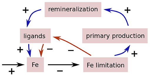
Figure 1. Illustration of the two feedback loops, one destabilizing (blue), the other stabilizing (red).
In the other scenario, as studied by Lauderdale et al. (2020), ligands are predominantly a by-product of the remineralization of particulate organic matter, such as pigments with porphyrin-like moieties that can bind iron. In that scenario, a reduction in iron supply could lead to a reduction in ligand production, possibly leading to runaway effect of decreasing iron, decreasing primary production, decreasing ligand concentrations. Again, an increase in iron supply would reverse the chain of reactions, and is shown as the blue arrows in Figure 1.
In the real ocean, both possibilities are probably realized; and there might be even compensations between them. But at the same time, the strength of this feedback will also crucially depend on the lifetime of the ligands. Iron limitation is only prevalent in some parts (albeit significant parts) of the global ocean. Depending on whether ligands in these regions are predominantly produced locally or have been transported from elsewhere, changes in iron limitation will affect the ligand concentration in these regions differently. From that one would expect that a longer lifetime leads to a smaller strength of the feedback. On the other hand, a longer ligand lifetime will also lead to a larger overall concentration of ligands, for a given ratio of ligands production to carbon fixation or any other measure of productivity, possibly increasing the feedback strength. In Lauderdale et al. (2020), it is actually the ratio between ligand production as part of biological production and the ligand degradation rate that controls the overall behavior of the system. Another possible control of the strength of the feedback will also be how fast non-ligand-bound iron is scavenged; unfortunately this is another property of the iron cycle for which we have only a limited theoretical understanding.
It should be noted, however, that a third possibility exists, namely that at least a fraction of the ligands present in seawater, though biologically produced, have essentially no connection to oceanic productivity. For example, the riverine input of terrestrial humic substances (HS) is an important source of HS observed in the ocean (Andrew et al., 2013). For the marine iron cycle they are of particular interest due to their high bioavailability (Lis et al., 2015; Blazevic et al., 2016) and long residence time (Catalá et al., 2015). Yet, their chemical composition is heterogeneous, leading to different binding stabilities with iron. Further, how the degradation on the transport pathway from river to ocean affects their binding stability remains unclear (Muller, 2018, and references therein). For this complexity and uncertainty, and since that terrestrial HS do not participate the ligand-related feedback, we ignore this source of ligands in our model and focus on the ocean-produced ligands in the analysis of the feedback strength.
The aim of this study is two-fold: We first investigate how different assumptions on ligand cycling affect the agreement to observations of phosphate and dissolved iron in a simple global model of ocean biogeochemistry (section 3). We then study the strength of the feedbacks mentioned above under idealized conditions, and determine how strongly it depends on our assumptions on ligand processes, such as the degradation lifetime of the ligand(s), but also on the strength and direction of the change in the external iron forcing (section 4).
2. Methods
2.1. The Model
It is currently not possible to fully explore the dependency of these feedbacks on parameters such as the pathways and rates of ligand production, their strength and lifetime, and the scavenging residence time with a full global biogeochemical and ocean circulation model. For this study we therefore represent the overturning circulation in the global ocean through a simple box model, with prescribed volume fluxes between the boxes, similar, but somewhat more complex than in Lauderdale et al. (2020), and assume that each box is well-mixed. The arrangement of the boxes is chosen to reproduce the main water masses in the deep ocean, and to separate the surface ocean into high- and low-latitude regions.
One aspect of the overturning circulation that we assume to be significant for the iron cycle with its relatively short residence time, is a distinction between the Atlantic and Indo-Pacific basins, with the North Atlantic being ventilated by North Atlantic Deep Water (NADW), in contrast to the Indopacific, where Deep Water is formed mostly through diapycnal diffusion from Antarctic Bottom Water (AABW). Fe does not show the increase of concentration along the path of the deep overturning circulation as phosphorus does, an effect that cannot be represented in a model with just one deep ocean box.
At the surface (which we for simplicity define as the upper 100 m), we distinguish in each basin between a northern box, extending from 70 to 24 N, and a tropical box from 24 N to 32 S, connected by a common Southern Ocean subpolar/polar box. At depth we distinguish, again for each basin separately, between one box ranging from the upper thermocline to Antarctic Intermediate Water AAIW (with a lower interface at σ0 = 27.3), one intermediate depth box for deep water, and one (σ4 > 45.86) for Antarctic Bottom Water. Finally we have one deep Southern Ocean box, below 100 m and south of 50 S. In total we thus have 12 boxes, whose arrangement is shown in Figure 2. The volume and surface area of the boxes (Table 1) have been estimated from hydrographic data from the World Ocean Atlas 2009 (Antonov et al., 2010; Locarnini et al., 2010).
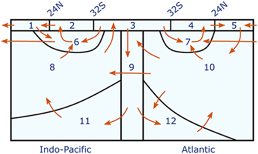
Figure 2. Schematic representation of the box model and the advective fluxes between the boxes. Also shown is the numbering of the boxes; names of the boxes are documented in Table 1. The strength of the advective fluxes and their relation to water mass transformations is documented in Table 2.
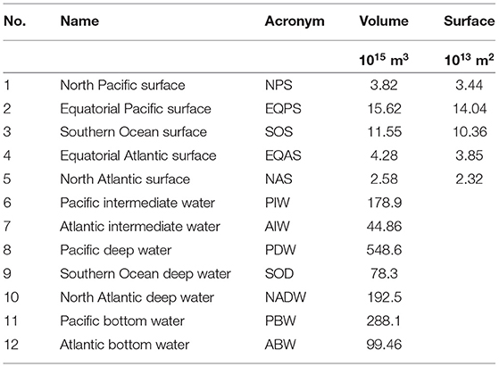
Table 1. Properties of the model boxes.
We base the volume fluxes between our model boxes (Table 2) on the recent analysis of the large-scale overturning circulation by Talley (2008, 2013), who emphasize that in the Southern Ocean, NADW upwells at a higher density and below Indopacific Deep water (IDW), and that NADW mostly gets transformed into AABW, while IDW splits into a part that enters AABW and a part that feeds the subtropical thermocline waters. Some additional information on fluxes in the near-surface water masses has been taken from Cerovečki et al. (2011), and the rate of NPIW formation of 6 Sv is from Talley (1997).
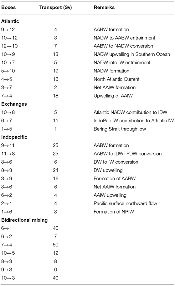
Table 2. Advective fluxes between the model boxes, and their relation to water mass transformation rates.
Compared to the overturning scheme of Talley (2013) we have changed one important detail: Talley (2013) argues that the decrease of the southward NADW flux from 24 N to 32 S by about 5 Sv, and the increase of the northward thermocline flow from 32 S to 24 N by about the same amount reflects a diffusion-induced transfer of water mass from NADW into the thermocline layer. In our simple box model, this diffusive transfer can only be represented by an advective term.
It is important to note that the fluxes from Talley (2008, 2013) are partly understood as purely advective and thus adiabatic (such as the upwelling of deep waters in the Southern Ocean), but also partly as resulting from diapycnal processes, such as the conversion from AABW to PDW and IDW in the Pacific basin. In our model, all these fluxes are represented as advective.
In addition to the overturning fluxes a mixing exchange between the top and the directly underlying boxes represents the nutrient fluxes caused by the annual mixed layer cycle and enhanced diffusion in the upper ocean.
Overall, the representation of the ocean circulation in the model can be considered an extension of the model by Parekh et al. (2004) to include some distinction in deep and intermediate water masses, and some newer insights in the structure of ocean overturning.
In each of these boxes, mass balances for phosphate, for the semilabile part of dissolved organic phosphorus, for iron, and—depending on scenario—for zero, one, or two organic ligands are solved. Lauderdale et al. (2020) uses nitrate rather than phosphate as the modeled macronutrient, but as long as constant stoichiommetry in organic matter is assumed and N2 fixation and denitrification are not modeled, this should not make a difference. The equations for phosphate, dissolved organic phosphorus (in the following also abbreviated as DOP), and for iron are
where P stands for the total inorganic phosphate concentration (in mmol m−3), D for the DOP concentration (in mmol m−3 as well), F for the dissolved iron concentration (in μmol m−3), and the indexes i, j enumerate the model boxes. Vi is the volume of a specific box, and the off-diagonal elements of the matrix Tij stand for the volume transport into box i from box j. The diagonal elements Tii, contain the total volume flow out of a box (a negative number). The term Ui describes the biological uptake rate of phosphorus by phytoplankton, of which a constant fraction ends up in DOP, while the rest is assumed to produce sinking organic particles. The Ui term is non-zero only in the surface boxes, i ≤ 5, and is parameterized following Parekh et al. (2004) as a linear function of phosphate and a saturating function of dissolved iron,
A fraction γ·Ui of this uptake is routed into DOP, which is then remineralized back to phosphate with a constant rate κ. The remaining fraction (1 − γ) · Ui of the uptake produces sinking organic particles which are instantaneously remineralized in the boxes located below a certain surface box. The source of phosphorus from this remineralization Ri is described by
such that the matrix elements rij are non-zero only if box i is located below box j, and . This ensures that for phosphorus the ocean is a closed system, i.e., the total amount of phosphate and DOP is conserved, but still leaves some freedom, as in our model surface boxes are located above several subsurface boxes. Our choice of the rij reflects the decrease of POC flux with depth (Martin et al., 1987) and is documented in Table 3.
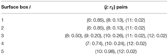
Table 3. Fraction rij of the export production from surface box i that is remineralized in deep-water box j.
Iron is cycled along with phosphate, assuming a constant Fe:P ratio ρ in biomass, but has an additional loss process, scavenging, and external sources. Total dissolved iron simulated in the model includes a truly soluble and a colloidal fraction. Kinetics of the formation and dissociation of colloidal iron is ignored and it is assumed that both fractions bind with ligands and are taken up by phytoplankton. The rate of loss of iron from scavenging is assumed to be a product of a scavenging rate α and the “free inorganic” fraction of dissolved iron F⋆ (often denoted as Fe'). The latter is calculated from the total dissolved iron concentration and the ligand concentration(s), as described further below. As external sources for iron, represented by Si in Equation (3), we take into account dust, sediments and hydrothermal sources. Dust flux has been calculated by integrating the annual mean dust flux from Mahowald et al. (2003) over the five surface boxes, and assuming a fixed solubility of the deposited iron. To take into account that fresh Saharan dust has a lower solubility that the estimated global average, we set the solubility in the equatorial Indopacific box (which is dominated by dust input from the Sahara and local sources into the Indian Ocean) to 0.25%, in the equatorial Atlantic box to 0.5%, and to 1% in all other boxes. A more mechanistic description of dust iron solubility might be possible (Baker and Croot, 2010; Meskhidze et al., 2019), but is hard to constrain in the simplistic box-model geometry used here. Flux of iron from sediments is assumed to be proportional to area of shelves with depth <1,000 m, calculated from the ETOPO2v2 data base, multiplied with a depth-dependency taken from Aumont et al. (2015); however, we chose a smaller maximum flux of 0.1 μmol m2 d−1. The strength of sediment iron fluxes into the ocean still differs substantially between models (Tagliabue et al., 2016) and is related to the chosen scavenging assumptions. Hydrothermal iron flux has been calculated from the source field for primordial 3He used in Tagliabue et al. (2010) and is added as a source to the model boxes depending on the total integrated flux into a box, assuming a Fe:3He-ratio of 9·105 mol mol−1. With these choices, the total input of dissolved iron from the different sources is dust: 8.18·108 mol yr−1, sediments 7.55·108 mol yr−1, and hydrothermal 8.48·108 mol yr−1.
We distinguish between three different treatments of iron-binding ligands. In the first, abbreviated CL in the following, ligand concentrations are set to a constant value Lconst (defined in Table 4) globally, an approach that is still followed in the majority of all global biogeochemical models (see, e.g., Tagliabue et al., 2016). In both other approaches, ligands can vary and one or two additional equations for ligand concentrations are solved. The equation of the DOC-related ligand is of the form
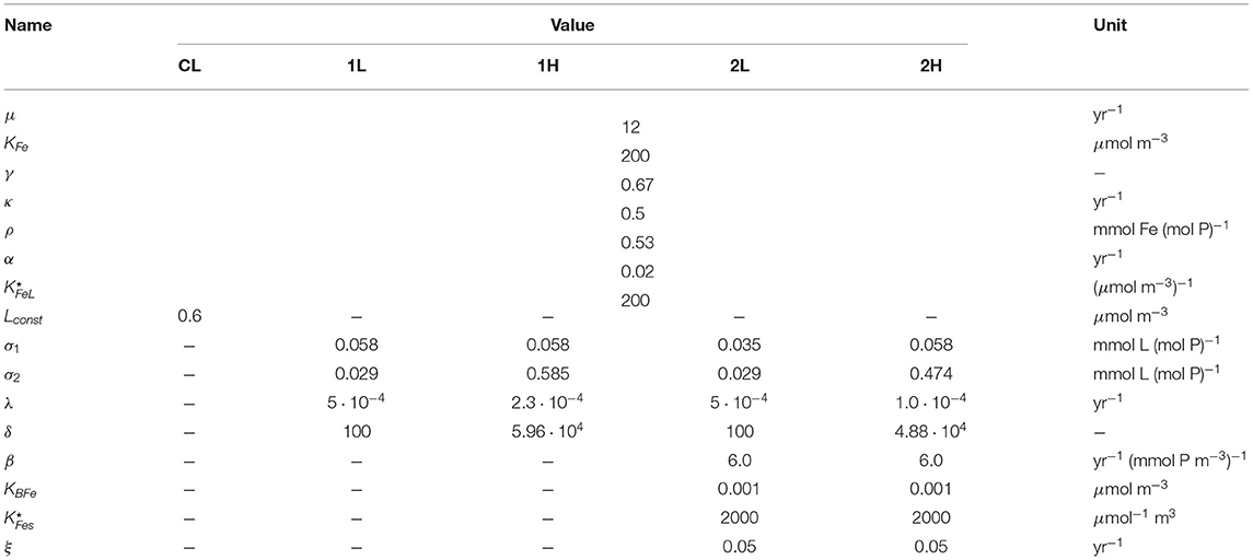
Table 4. Biogeochemical parameters of the model; where more than one value appears in a row, the first is for the constant-ligand case (CL), the second and third for the case with one DOC-type ligand (1L and 1H), and the other two for the two different cases with both a DOC-like and a siderophore-like ligand (2L and 2H).
Here, L stands for ligand concentration (in μmol m−3), λi is the ligand degradation rate, σ1 is the proportionality factor between biological phosphorus uptake and ligand production, and σ2 is the proportionality factor between phosphorus remineralization from organic particles and ligand release. The values chosen for the ligand-related parameters are discussed in section 3.1. Both source terms reflect that in the breakdown of organic matter strong iron-binding functional sites are produced, either from functional groups present in the precursor particulate material, or in the substrates produced by the degrading bacteria (Boyd et al., 2010). The model is a simplified version of the ligand model by Völker and Tagliabue (2015), the main difference being that the ligand degradation rate below the surface is constant, with a degradation rate λi = λ, while it is higher by a factor of δ in the surface boxes λi = δλ, due to photodegradation, like in the model by Lauderdale et al. (2020). In Völker and Tagliabue (2015) λ was made dependent on ligand concentration, in order to describe a continuum of faster and slower degrading ligands.
As siderophores are rather small and nitrogen-rich molecules, they are likely to be more quickly consumed by bacteria as food, and cannot explain the presence of ligands in the deep ocean. We treat them as an additional ligand, with a distinct production pathway. Our assumptions are that siderophores are produced proportional to the concentration of semi-labile DOP, which we take as an indication of bacterial food, and that its production is regulated by iron limitation, i.e., tends to zero as iron concentrations approach non-limiting conditions for bacteria. We further assume that siderophores are broken down by bacteria at a constant rate ξ. With these assumptions, the equations for siderophore concentrations Si (in μmol m−3) are
Here, β is the proportionality between DOP concentration and siderophore production, and KBFe is a half-saturation constant for bacterial iron limitation.
Depending on whether we model siderophores or not, the calculation of the “free,” i.e., uncomplexed iron concentration differs. In the case that only one ligand is present, the calculation reduces to the solution of a second-order equation, as already described by Parekh et al. (2004). In the case that siderophores are present, one has to solve three mass balances describing the distribution of iron and of two ligands into the free and ligand-bound forms, as well as the two chemical equilibria. In the end, this reduces to a third-order equation for free iron alone, with only one real positive solution. We assume that the conditional stability constant for iron binding by siderophores, is larger by an order of magnitude than that of the DOC-related ligand .
The model is freely available via github (Völker, 2021). It is written in the MATLAB computing language, and we have used the ode23s routine for solving stiff differential equations, which is based on a Rosenbrock formula of order two (Shampine and Reichelt, 1997), to integrate it forward in time. One integration of the model over 5,000 model years typically takes a second on a generation 2015 Intel MacBook.
2.2. Model Assessment
After setting the model parameters to one of the five scenarios described further below (section 3.1), the model is integrated 20,000 years, until concentrations in the individual boxes have converged to a near-steady state. Model results are compared to concentrations of phosphate and iron that are representative for each box. For phosphate, for which a good global data coverage exists, the representative values are simply the average concentrations within each box, calculated from the climatology provided by the World Ocean Atlas 2009 (Garcia et al., 2010). For iron the data coverage is presently not good enough to form a global climatology. Furthermore, although iron concentrations in the deep ocean are typically below 1 nmol L−1, and often below 0.1 nmol L−1 near the ocean surface, very high values (>50 nmol L−1) have been found in the vicinity of hydrothermal vents. For both reasons, the mean of observations is not a good representative of typical concentrations. We have therefore chosen the median Fe concentration of all observations within each box from the GEOTRACES second intermediate data product (Schlitzer et al., 2018) as representatives.
2.3. Quantification of Feedback Strength
The strength of the feedback between changes in the iron cycle and ligand concentrations can be evaluated in a manner similar to the analysis of feedbacks between climate change and the carbon cycle (Hansen et al., 1984; Friedlingstein et al., 2003): Starting from an equilibrium solution of the coupled phosphorus-iron-ligand system, the iron cycle is perturbed, e.g., by changing external iron sources such as dust deposition, and the resulting changes are followed twice, once with the full model, and once keeping the ligand distribution at the previous equilibrium state.
Let E be a quantity that we are interested in, or in an abstract way of speaking our “metric.” In the case of the ocean iron cycle, the metric could be the total ocean inventory of iron, but also any other quantity related to it, such as the global export production. Also let F be the “driver,” i.e., the quantity that is disturbed, which in our case could be the total flux of iron into the ocean from dust deposition. Then, for the unperturbed state, we define E0 = E(F0) the equilibrium value of E for the unperturbed driver F0, obtained from our model. As we perturb the driver by F = F0 + ΔF, we will also obtain a changed value of the metric, which we may linearize as E = E0 + ΔE. We define
where ΔE is the equilibrium change that is obtained running the full model including the feedback that we want to analyze, and ΔE0 is the change that we obtain when in the model we exclude the feedback. The quantity f is known as feedback factor. The system gain g is defined as the effect of the feedback, ΔEfb = ΔE − ΔE0, divided by the change in the metric excluding the feedback, i.e., g = ΔEfb/ΔE0. The relation between f and g is then
A positive value of g, and hence f>1, stands for a positive feedback, while a negative feedback implies a negative value of g and hence f < 1.
We focus in the following on the feedback with respect to changes in global dust deposition. For the analysis of feedbacks, the models including prognostic ligands are run several times: First the model is run once with standard dust deposition, to obtain the steady-state ligand distribution. Then the model is run into steady state for a range of different total dust deposition values, keeping ligand concentrations held at the values from the unperturbed run. And finally, the model is run again into steady state for different dust deposition values, but allowing the ligand distribution to change due to the new conditions. While the feedback factor f and system gain g are based on linearization and are therefore best calculated with small changes in dust deposition, we also investigate the nonlinear response by varying the dust deposition from zero to two times the standard deposition.
Different variables in the box model are affected differently by the feedback through production of ligands. We choose a small set of four globally relevant quantities as metrics to measure the response to the perturbation: The first is the globally averaged concentration of dissolved iron in the ocean. The second is the average concentration of dissolved iron in the surface boxes, where it affects biological production. The third is the dissolved iron concentration in the surface Southern Ocean, which is the largest iron-limited region. And finally the fourth is the global export production, as a measure of biological activity.
3. Assessment of the Unperturbed Models
3.1. Ligand Parameter Choices
Several of the parameters that describe the cycling of the ligand(s) in the model are not well constrained from observations, although an order of magnitude estimate for some can be inferred from observational data. Here we explain, how they were chosen, all parameter values used in this study are documented in Table 4. Estimates for the ligand:phosphorus (or ligand:carbon) ratio in the remineralization of organic matter σ2 have been derived in Völker and Tagliabue (2015) and Lauderdale et al. (2020). Völker and Tagliabue (2015) also estimated an order of magnitude on the order of a millennium for the ligand degradation timescale 1/λ in the deep ocean.
We attempted to constrain the remaining parameters from an optimization of the model with respect to agreement with the iron observations. It turned out, however, that the data is not enough to constrain all parameters independently. While deep-ocean observations put some constraints on the parameters governing the long-lived DOC-type ligand (Equation 6), there is considerable ambiguity for the parameters for the shorter-lived siderophore-type ligands described in Equation (7). In consequence the optimization procedure often spent long periods in search for minimal gains in model-data agreement by co-varying parameters, ending with parameter combinations that made not much sense from a biogeochemical point of view.
We therefore opted for a pragmatic approach and hand-tuned the parameters to some extent within bounds judged to be reasonable in our opinion. To obtain an estimate of the parameter-related uncertainty we present here four different setups or scenarios for modeling ligands: The first of these has only one long-lived ligand, and parameters resemble the settings in Völker and Tagliabue (2015) and Lauderdale et al. (2020). This setup is referred to in the following as 1L.
A known problem with this setting of parameters is that even with a ligand degradation timescale of 2000 years, the deep Pacific becomes too depleted in ligand, and hence dissolved iron. A possible explanation for this discrepancy to observations is that the model misses a part of the very long-lived or refractory component of dissolved organic carbon (Gledhill and Buck, 2012, e.g., humic acids) which can also act as iron-binding ligand. To account for this possibility within our simplistic description of ligand cycling, we also studied a setup with ligand degradation timescale on the order of 5000 years. This is significantly longer that the estimate of the turnover time of fluorescent dissolved organic matter by Catalá et al. (2015), but on the order of the largest dissolved organic radiocarbon ages (Hansell, 2013). It turns out that in this setup (1H) we had to simultaneously increase the ligand:phosphorus ratio in the remineralization source of ligand by a substantial amount, and also increase the photochemical breakdown rate of the ligand.
To these two setups we add two more, that are similar in their settings of the DOC-like ligand parameters, but include a shorter-lived siderophore-like component. We chose a degradation timescale for these ligands (parameter 1/ξ in Equation 7) that is two orders of magnitude smaller than that for the other ligand. One would probably assume even faster bacterial degradation rates for true siderophores, which are small and nitrogen-rich organic molecules, but these cannot reasonably be represented within a box model, representing the circulation at timescales of decades or longer. Additionally, we reduced the production of long-lived ligand in surface boxes (parameter σ1, see Table 4), in order to avoid overly high surface total ligands and hence dissolved iron. The two setups with two prognostic ligands are denoted by 2L and 2H in the following. The parameters for all five setups (including the constant ligand case CL) are documented in Table 4.
All of the five model runs (CL, 1L, 1H, 2L, and 2H) reproduce the global patterns of phosphate (Figure 3) and iron (Figure 4) concentrations, with an overall slightly better fit by the models with prognostic ligands (see below and in the Supplementary Table 1, which shows that bias and root-mean-square difference between model and comparison data both for iron and phosphate are reduced in these runs). We acknowledge, however, that different parameter choices may still lead to further improvements.
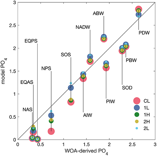
Figure 3. Phosphate concentrations for the 12 model boxes from model results (y-axis) vs. mean concentrations derived from World Ocean Atlas data (x-axis). Acronyms for the model boxes are defined in Table 1. Red dots show results from the model with constant ligand concentration (run CL), blue and dark green from the model with one prognostic ligand (runs 1L and 2H), and yellow and cyan from the two model runs with two prognostic ligands (runs 2H and 2L, respectively). Symbol sizes have been made different to show all values, even if they are close.
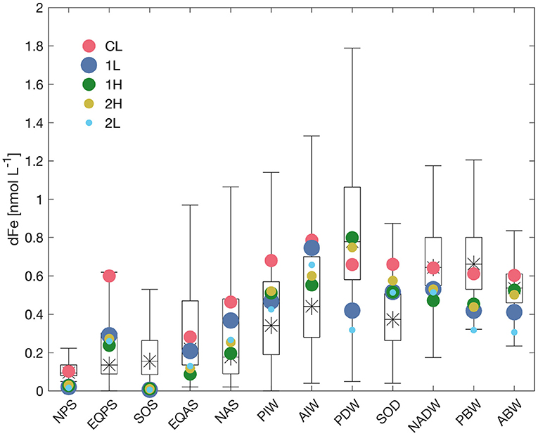
Figure 4. Dissolved iron concentrations for the 12 model boxes from model results (colored dots) vs. derived from GEOTRACES IDP2 data (boxplots). The star shows the median concentration from the observations, the box ranges from the lower quartile to the upper quartile, and the lines extend to a length of 3/2 the interquartile range or to the maximum or minimum of the data (whichever is smaller) above the upper or below the lower quartile. The more extreme dissolved iron concentrations from stations near hydrothermal vents enter in the calculation of the quantiles, but are not shown in the whiskers. Red dots show results from the model with constant ligand concentration (run CL), blue with one prognostic ligand (run 1L), green from the model run with one very long-lived ligand (run 1H), and yellow and cyan from the model runs with two prognostic ligands (run 2H and 2L, respectively).
A comparison of the model distribution of phosphate and iron with output from two full three-dimensional global biogeochemical models is shown in the supplement. All box model runs have a global export production that is on the low end of data-based estimates, with 6.68 PgC yr−1 (CL), 6.05 PgC yr−1 (1L), 6.30 PgC yr−1 (1H), 5.80 PgC yr−1 (2L), and 6.40 PgC yr−1 (2H).
3.2. Constant Ligand, CL
The modeled phosphate concentrations in the steady state of the model are plotted as red dots in Figure 3 vs. the average phosphate concentration in the boxes, calculated using the World Ocean Atlas data (Garcia et al., 2010). It is conceivable that most model-data points cluster around the 1:1 line, i.e., that overall the model describes the global distribution of phosphate reasonably well. A small but systematic error concerns the five surface boxes, where phosphate concentrations are lowest. In all surface boxes, the model underestimates phosphate concentrations, and the largest deviation is in the surface North Pacific box, which from WOA has an average phosphate concentration of 0.73 μmol L−1, while the model produces 0.18 μmol L−1.
The comparison is less straightforward for dissolved iron (dFe). Due to the inhomogeneous distribution of observational data for iron, we have plotted modeled dFe concentrations against the median and quantile information available for each model box from GEOTRACES data (Figure 4, red dots). Relative deviations between model and data are larger than for phosphate, but part of these deviations may also be due to the incomplete sampling for iron. Surface iron concentrations are too low in the North Pacific and Southern Ocean, similar to those of phosphate. Else, the concentrations in the surface and intermediate water masses have a tendency for overestimation by the model (especially so in the Equatorial Pacific box, probably because of the high dust deposition near the African continent in the Indian Ocean, that gets counted as iron input into this box, but hardly influences dFe concentrations in the equatorial Pacific, where most measurements took place), while the deep ocean concentrations are surprisingly close to observations, except for the deep Southern Ocean, which has a too high dFe concentration in the model. Overall, dFe concentrations show less variation between the different deep water masses in the model, compared to the observations, a tendency known from full three-dimensional ocean biogeochemistry models with constant ligands (e.g., Tagliabue et al., 2016).
3.3. One DOC-Type Ligand, 1L and 1H
The modeled steady-state phosphate concentrations from the DOC-based ligand model 1L, which are compared in the blue dots in Figure 3 to the data-based box averages, agree better with the observations than the concentrations modeled with constant ligand concentration: The systematic error of too low surface phosphate concentration in the surface boxes is almost gone, and especially the Southern Ocean and North Pacific surface boxes are now much closer to data. There are also slight improvements in almost all deep ocean phosphate concentrations, compared to the case with constant ligands, which may be due to better pre-formed phosphate concentrations in the surface boxes.
Phosphate concentrations in the model run 1H with one, very long-lived and more photolabile ligand are shown as green dots in Figure 3. They are in between those from runs 1L and CL, i.e. they are slightly less good than in the 1L run, but better than in CL. The one exception is the equatorial Atlantic surface box, where the long-lived ligand case leads to higher phosphate, in better agreement with observations.
Dissolved iron concentrations from the model run 1L, shown as blue dots in Figure 4, are somewhat closer to observations than in the CL run in the surface and intermediate water boxes, but concentrations in the deep and bottom water boxes are generally lower than in the constant-ligand case. While this brings the model closer to observations in the Southern Ocean, it leads to clearly too low dFe concentrations in the deep Pacific boxes. This pattern has already been observed in the first global biogeochemical model with prognostic ligands (Völker and Tagliabue, 2015), and is due to the old ventilation age of these water masses, combined with the fact that within these water masses there is comparatively little direct ligand production from the remineralization of particulate organic matter. Both lead to low ligand concentrations in these boxes (blue bars in Figure 5) and hence stronger scavenging of iron.
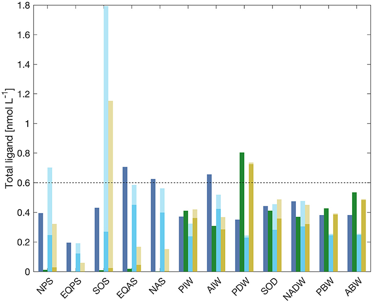
Figure 5. Equilibrium ligand concentrations in all model boxes for the model with one prognostic ligand (blue, run 1L), with one long-lived ligand (green, run 1H) and for the model runs with two prognostic ligands (cyan, run 2L, and yellow, run 2H). In the latter two, the lighter color stands for the siderophore-like ligand Si, while the darker stands for the longer-lived ligand Li. The dashed line shows the constant ligand concentration in run CL.
Iron concentrations in the run with a very long-lived ligand 1H, shown as green dots in Figure 4, are closer to observations than runs 1L in four out the seven sub-surface boxes, with in some cases drastic improvements (Atlantic Bottom Water, Atlantic Intermediate Water, and Pacific Deep Water boxes), where the model is also much closer to observations than the constant-ligand run CL. In the remaining three subsurface boxes, the agreement to observations is only slightly worse than in 1L. At the surface, the picture is somewhat mixed, with improvements, compared to both 1L and CL in the Equatorial Pacific and North Atlantic surface, a deterioration in the Equatorial Atlantic and hardly any change in the North Pacific and Southern Ocean.
3.4. DOC- and Siderophore-Type Ligand, 2L and 2H
The two cases with two prognostic ligands, one DOC-like and one siderophore-like 2L and 2H, are very similar to their corresponding runs with just one ligand in their distribution of phosphate and dissolved iron.
In both runs 2L and 2H, all phosphate concentrations are somewhat higher than in the corresponding one-ligand cases 1L and 1H, with one exception, which is the deepest Pacific box. This brings the model slightly closer to observations at the surface and in the deepest Pacific, while changes of model-data agreement in the other deep parts of the ocean are mixed (Figure 3, yellow and cyan dots).
In run 2L, the introduction of a second-siderophore-like ligand leads to a slightly better agreement with dissolved iron data, compared to 1L, in the intermediate waters and the North Atlantic surface box, but also to a decrease in iron concentrations in all deep and bottom water boxes, further widening the discrepancy to observations (Figure 4, cyan dots). This is due to the reduction in the production of long-lived ligand in surface boxes (parameter σ1, see Table 4) in setups 2L and 2H, which was made in order to avoid overly high surface total ligands and hence dissolved iron.
In run 2H, dissolved iron concentrations (Figure 4, yellow dots) are slightly higher than in run 1H (green dots) in all boxes except the Pacific Deep and the Pacific and Atlantic Bottom Water boxes. This brings the model very slightly closer to observations in some boxes but further away in others, but overall the changes are too small to consider them as significant.
The increases in dissolved iron concentrations in runs 2L and 2H, compared to their counterparts 1L and 1H, can be explained by the increase in total ligand concentrations with the introduction of a new shorter-lived ligand (Figure 5). It is interesting to note that although the degradation timescale for the shorter lived ligand is on the order of decades we still find a sizeable contribution of these ligands to the total ligand pool in the deep Southern Ocean and the North Atlantic Deep Water boxes. This is caused by water mass formation from surface water with elevated concentration of these ligands. In the context of a box model, such a ventilation affects the whole water mass instantaneously, while in the real ocean one would find a gradient within the water mass with increasing distance from the ventilation source.
4. Strength of Feedbacks
We perform a feedback analysis as described in section 2 for each of the models setups including prognostic ligands (1L, 1H, 2L, and 2H) separately.
4.1. One DOC-Type Ligand, 1L and 1H
All four chosen quantities, or metrics vary in the same direction as the variation in the dust deposition (Figure 6), regardless of whether the ligand feedback is excluded (dashed lines) or included (solid lines). The change in all quantities, however, is larger when the feedback is included than when it is not, reflecting the positivity of the feedback.
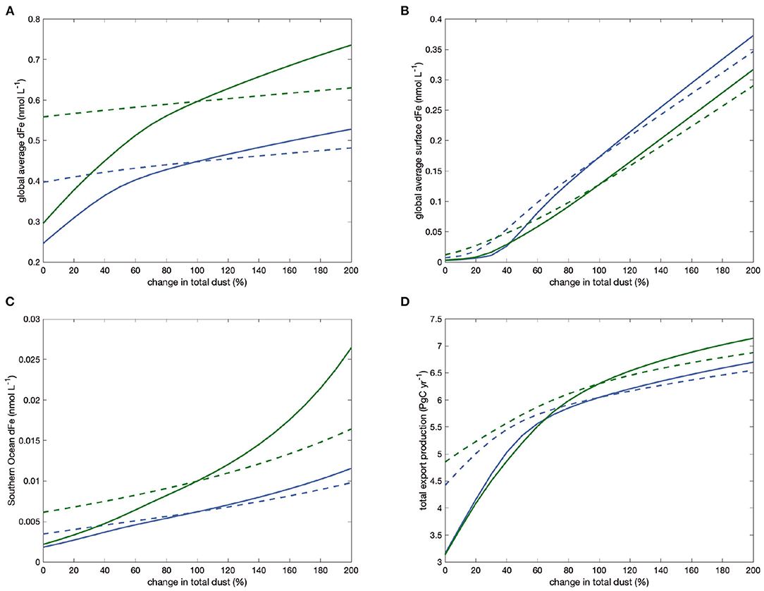
Figure 6. Changes in global average dFe concentration (A), surface-average dFe (B), Southern Ocean dFe (C), and global export production (D) in the model with only one DOC-type ligand, as the magnitude of the total dust is varied, including (solid lines) and excluding (dashed lines) the feedback through changes in ligand concentrations. Blue lines are for model run 1L, green for 1H.
The global average concentration of dissolved iron, shown in Figure 6A, behaves in a strongly buffered way when ligands are held constant at the state before perturbation (dashed lines), with a doubling of dust deposition leading only to a in increase of 0.034 nmol L−1 or 8% in run 1L and similar in run 1H. Allowing feedbacks by a variation of ligands from the background state (solid lines), the reaction of dissolved iron to a change in dust deposition becomes much stronger. The feedback factor f, which describes the ratio of the slope of the solid and the dashed curves for vanishingly small perturbations is more than 2.5 in 1L (blue lines) and even more than 4.7 in 1H (green lines). Generally, the longer lifetime of the ligand in run 1H, compared to 1L leads to a stronger effect of the feedback, as evidenced by the larger values of the feedback factor f and the system gain g (Table 5). A further observation concerns the curvature of the lines in Figure 6A: The effect of changing ligand concentrations (the difference between the solid and dashed lines) is stronger in scenarios with a reduction in dust deposition, as opposed to an increase. This is because the reduced ligand concentrations in these cases also increases the scavenging loss of iron that comes from hydrothermal or sediment sources. This then leads to an increase of iron limitation also in otherwise iron-replete regions and a further reduction in productivity.
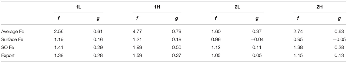
Table 5. Feedback factors f and gain g for the four chosen metrics in the four model runs with prognostic ligands 1L, 1H, 2L, and 2H.
The average surface dFe concentration, shown in Figure 6B, is much less well buffered and follows almost linearly the dust deposition, when ligands are held fixed, except at very low total dust. Consequently, the feedback effect of variable ligands is less pronounced, with a feedback factor f that is just slightly above one and a gain just slightly above zero for both model parameter settings 1L and 1H (Table 5). The surface average dFe concentration is dominated by the concentration in the subtropical boxes, which have the largest areas. In these boxes, dust deposition is the main supply of dFe and scavenging of iron is largest.
This is different in the two main iron-limited regions, the subpolar North Pacific, and the Southern Ocean, where iron supply from dust is smaller than from upwelling and vertical mixing. In the Southern Ocean (Figure 6C, therefore, dFe concentrations depend less on dust-deposition in the constant-ligand case. The variability of dust enhances the sensitivity of dFe concentrations to dust because it affects the production of ligands which in turn change the iron concentrations that upwell in the Southern Ocean. The feedback factor f and gain g are intermediate between those for global average and surface average dFe concentrations.
Finally, the changes in iron availability in the main iron-limited regions (Southern Ocean and North Pacific) also lead to corresponding changes in export production. The feedback factors f for export are 1.4 and 1.6 in 1L and 1H, slightly lower than to those for the Southern Ocean iron concentration. Again, the change in export caused by a reduction in dust deposition is much stronger than that caused by a corresponding increase when the feedback is included.
4.2. DOC- and Siderophore-Type Ligand, 2L and 2H
The feedbacks of the four quantities considered show a qualitatively similar pattern when a second, siderophore-type ligand with shorter life-time is introduced into the model (Figure 7): Again, there is an overall positive feedback that leads to a stronger variation of global average dFe with changing dust deposition when the ligands are allowed to react to the change, which reduces the otherwise strong buffering of global dFe (Figure 7A). Again, the feedback is larger for global average dFe and Southern Ocean dFe (Figure 7C) than for globally averaged surface dFe (Figure 7B) and export production (Figure 7D). And again, the feedbacks are stronger in the case with a more long-lived DOC-type ligand (parameter set 2H, yellow lines) than with a somewhat shorter-lived DOC-type ligand (parameter set 2L, cyan lines).
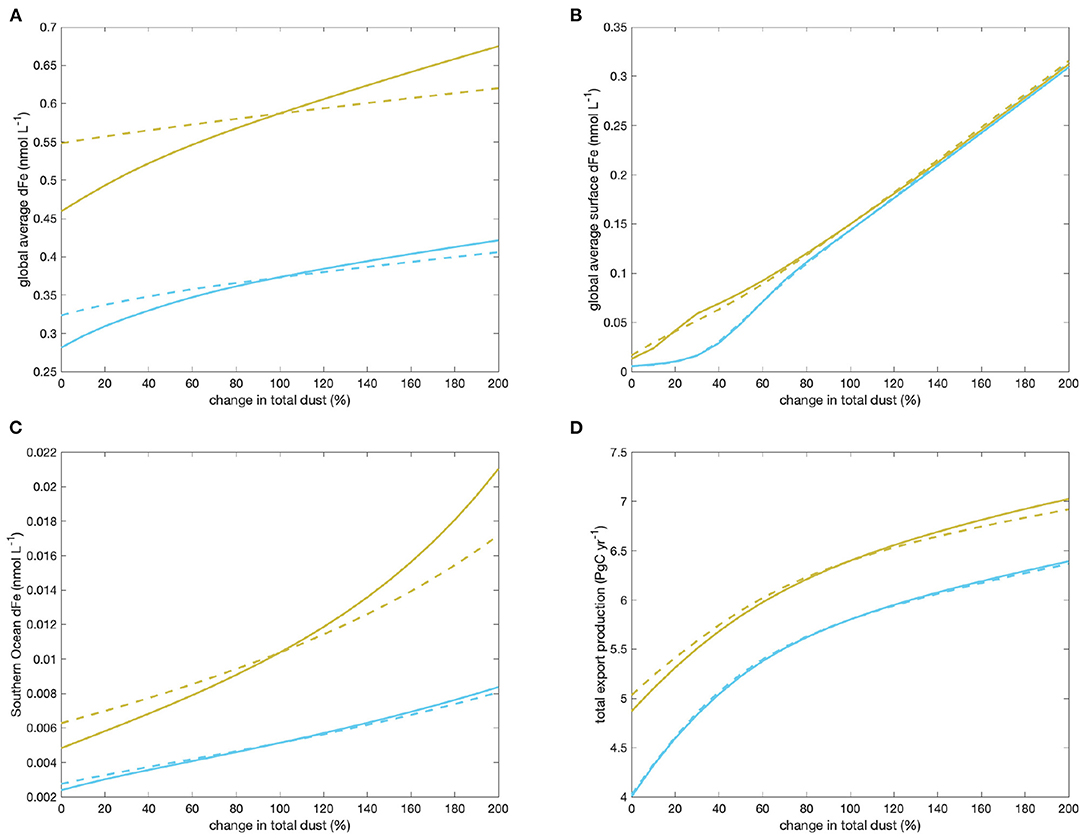
Figure 7. Changes in global average dFe concentration (A), surface-average dFe (B), Southern Ocean dFe (C), and global export production (D) in the model with two types of ligands, as the magnitude of the total dust is varied, including (solid lines) and excluding (dashed lines) the feedback through changes in ligand concentrations. Cyan lines are for model setup 2L, yellow for 2H.
The strength of the overall positive feedback, however, is greatly reduced when a second siderophore-type ligand is modeled as well, as indicated by the smaller values of f and g in Table 5. Feedback factors in cases 2L and 2H are about 60% of those in the corresponding case with only one ligand 1L and 1H for global average dFe, and between 70 and 80% for Southern Ocean dFe. For global surface average dFe there is even a very small but overall negative feedback, as indicated by values of f slightly below one. As global export production is tied to surface dFe concentrations, its feedback is weak but positive, indicating that the increase of export production in the Southern Ocean with increasing dust is partly offset by decreases in other ocean regions.
It is obvious that the introduction of an additional negative feedback loop with siderophore-type ligands will to some extent counteract the strength of the positive feedback loop with DOC-type ligands. That the overall feedback still stays positive and the pattern of feedbacks reflects the relative role of the different ligands in runs 2L and 2H: The global average iron concentration is dominated by the deeper ocean boxes, where the siderophore-type ligand is less abundant due to its shorter lifetime, and the DOC-type ligand determines iron solubility. And since global export production increases with increasing dust deposition (albeit with only a very small feedback), these ligands increase as well. In the surface, however, iron solubility is determined by both ligands, and hence the feedbacks can partly cancel out. This then makes the feedback in export production small.
5. Summary and Discussion
In this study we used a simple box model to investigate possible consequences of the fact that the solubility of iron in the ocean is to a large degree determined by the complexation with organic ligands. Since ocean-sourced ligands themselves are a (by)product of biological activity, which depends on iron availability, this creates the possibility of feedbacks that affect how the oceanic iron cycle reacts to changes, such as in the strength of external iron sources. Unlike full three-dimensional global biogeochemical models, the description of many processes is extremely simplified in a box model or even missing. It allows, however, to perform a large number of model runs quickly, so that feedback studies can be performed.
We compared three scenarios for how the production of ligands depends on biological activity: In the first, the concentration of ligands is globally constant and does not depend at all on ocean productivity; this is what most global biogeochemical models of the iron cycle still assume and would correspond to the ligands being part of the very refractory pool of long-lived dissolved organic carbon in the ocean.
In the second scenario, the ligand is produced or released during the degradation of particulate organic matter, as has been inferred from parallel measurements of DOC and ligand (Wagener et al., 2008; Schlosser and Croot, 2009) and has directly been observed in the experimental study of Boyd et al. (2010). This scenario also forms the basis of the study by Lauderdale et al. (2020). For this scenario to be compatible with measured vertical profiles of ligands they must on average have orders of magnitude shorter life-times in the near-surface ocean, for example through photodegradation (Powell and Wilson-Finelli, 2003), than in the deep ocean.
In the third scenario, an additional siderophore-type ligand is produced in response to iron limitation (Wilhelm and Trick, 1994; Boiteau et al., 2019), either to enhance a bacterial species' iron uptake, or to prevent its loss to other species or to precipitation.
A first set of results shows that the models reproduce the observed distribution of phosphate somewhat better with explicit description of organic ligand cycling than without, especially in the Southern Ocean and North Pacific surface, but also to some extent in intermediate and Pacific deep and bottom waters. For iron the picture is somewhat mixed, with the models with prognostic ligands improving the fit to observations in most surface and intermediate waters, and in the deep Southern Ocean, but deteriorating it in the deep and bottom waters of both Atlantic and Pacific. Overall, a prognostic description of ligands leads to a lower mean average error and bias in the iron distribution (Supplementary Table 1). The reason for the mismatch in the deep ocean boxes are the modeled low ligand concentrations there, which may be an artifact of neglecting the possible role of very refractory humic-like ligands (Laglera and van den Berg, 2009; Whitby et al., 2020) or carboxyl-rich alicyclic matter (CRAM) (Hertkorn et al., 2006). Other approaches to represent the DOC-related component of iron-binding ligands have been suggested (Ye et al., 2020), and may need to be pursued further.
The model parameters that describe the cycling of ligands are not well constrained from measurements, and like Lauderdale et al. (2020) we find that observations of phosphate and iron concentrations are compatible with a wide range of parameter settings, especially when adding a siderophore component to the model. The principle of parsimony might thus be taken as an argument to at least leave away the siderophore component, i.e., our third scenario. Siderophores, however, do exist in the ocean (e.g., Mawji et al., 2008; Boiteau et al., 2019), and we have instead decided to represent them here, because they may affect the direction and strength of the feedback to changing iron inputs. A more exhaustive exploration of the parameter sensitivity would have been possible, and we realize that the timescale of ligand degradation in the model set-ups 2L and 2H is probably too long for simple nitrogen-rich molecules such as many siderophores. However, we think that timescales shorter than a decade are not adequately represented in our box model anyway and have therefore not pursued this further.
In our model setup, siderophores only influence the solubility of iron, but not its bioavailability. It has been shown that eukariotes like diatoms have difficulties taking up siderophore-bound iron (Lis et al., 2015), although some species possess Fe-siderophore specific reductases (Maldonado and Price, 1999; Coale et al., 2019). Our model assumption is that the ecological aspect of siderophores, making iron exclusively available to a part of the microbial spectrum, is more important on shorter time-scales, and that on the long time scales relevant for the box model, siderophore-bound iron eventually becomes bioavailable. This clearly is an assumption that merits further study.
Modeled total ligand concentrations in Figure 5 are generally on the low end of observed ligand concentrations (e.g., Buck et al., 2015), although a full comparison is not yet possible, due to the scarcity of in-situ ligand measurements. This is a general issue; most models presented in Tagliabue et al. (2016) use a fixed ligand concentration of 1 nmol L−1. Ligand concentrations in models are tuned in to obtain a reasonable deep ocean iron concentration, and are therefore influenced by simplifications in the models, such as the assumption of a single conditional stability constant of the ligand, and the absence of less ligand-reactive components of iron, such as nanoparticles.
The main reason for presenting different setups of a ligand cycling model (model runs 1L, 1H, 2L and 2H) is that they, despite all about equally well reproducing phosphate and dissolved iron, show somewhat different patterns of feedbacks when the external iron input from dust deposition is varied. In the one-ligand model scenarios (1L and 1H) the feedback is positive, i.e., the reaction in iron concentrations and productivity to a change in iron input is enhanced, because the change leads to a concomitant change in ligand concentration. In the two-ligand scenarios (2L and 2H), the negative feedback from siderophores counteracts the positive feedback to some extent, despite the short life time of the siderophores. This is because the siderophores help buffer production in iron-limited regions, they make export production less dependent on external dust changes; and that then means that the production of DOC-like ligands does not change much. The positive and negative feedbacks mostly cancel for the surface iron concentration and global export production, but the positive feedback prevails for the global average and Southern Ocean iron concentrations.
Although siderophores have not only been found in surface layer, but also in the mesopelagic ocean at depths of 1,500 m, it is generally assumed that they have been produced in place (Bundy et al., 2018; Boiteau et al., 2019). Our personal assessment is therefore that the lifetime of siderophore-type ligand in experiments 2L and 2H is possibly still an overestimate, and that consequently, the positive feedback related to the DOC-like ligands is likely to dominate over the negative feedback associated with the siderophore-like ligands. Further studies on the mechanisms that lead to loss or breakdown of siderophores in the ocean would be needed to make this statement more conclusive.
It has been argued (Lauderdale et al., 2020) that the feedbacks between iron availability and ligand production bring the system to a state where there is “just enough” iron so that overall the production is limited by the macronutrient phosphate, and that iron limitation only occurs in remote parts of the ocean. This assessment was based on considering the positive feedback only. Interestingly, with our model we basically arrive at the same conclusion, when we assume that siderophore-type ligands have a shorter lifetime than the less specific ligands produced in the breakdown of organic matter.
In this study we have limited ourselves to feedbacks that act via the direct influence of ligands and iron on biological productivity. Our model therefore does not describe the input of terrestrial humics from rivers and the parameterization of long-lived ligands is based toward marine humics. This leads to two shortcomings: firstly, the missing of localized sources of terrestrial humics by the Arctic rivers (Krachler and Krachler, 2021) certainly affects the iron concentration in the Arctic Ocean. The global effect of the source localization is small, given the long lifetime of these substances. Secondly, unlike the other long-lived ligands, terrestrial humics are not tied to marine production. Neglecting this fraction of ligands is therefore likely to lead to some overestimate of the feedback strength in this study. Another possible feedback connects iron with the total inventory of nitrogen in the ocean, both through the high iron requirement of N2 fixation and through iron-related changes of oxygen minimum zones and hence denitrification (Falkowski, 1997). This feedback is neglected here, but would be an interesting subject for a follow-up study.
Our results have implications for possible reactions of the global carbon cycle to historical or predicted changes in dust deposition. Many ocean biogeochemical models have shown rather modest changes in reaction to a glacial increase in dust (e.g., Tagliabue et al., 2009; Lambert et al., 2015; Muglia et al., 2017), to anthropogenic changes in dust production or dust iron solubility (e.g., Krishnamurthy et al., 2009; Wang et al., 2015) or to deposition of iron with pyrogenic aerosols (Ito et al., 2021). To some extent this is to be expected, since the iron content in the ocean is buffered by the presence of organic ligands. But, with few exceptions, e.g., Hamilton et al. (2020) and Ito et al. (2020), these model studies have all been performed with models that fix the ligand concentration in the ocean and hence disregard possible feedbacks through changes in iron solubility.
Here we have shown, that the positive feedback also leads to an enhanced sensitivity of the biological production and hence the carbon cycle to changes in external iron supply, relative to a state that is buffered, but where the buffering undergoes no changes. We therefore argue that models that assume constant ligand concentrations (in effect representing the effect of the feedback on the background state, but not on changes), may underestimate the effects on the carbon cycle.
Data Availability Statement
Publicly available datasets were used in this publication. The model to produce the output shown can be found at doi: 10.5281/zenodo.5068784.
Author Contributions
CV and YY designed the study and wrote the manuscript. CV wrote the model and performed the model experiments. Both authors contributed to the article and approved the submitted version.
Funding
CV received funding for this research from the European Union's Horizon 2020 research and innovation programme under grant agreement No. 820989, project COMFORT. The research work by YY was funded by the DFG (German Research Foundation) project YE170/2-1.
Conflict of Interest
The authors declare that the research was conducted in the absence of any commercial or financial relationships that could be construed as a potential conflict of interest.
Publisher's Note
All claims expressed in this article are solely those of the authors and do not necessarily represent those of their affiliated organizations, or those of the publisher, the editors and the reviewers. Any product that may be evaluated in this article, or claim that may be made by its manufacturer, is not guaranteed or endorsed by the publisher.
Acknowledgments
We thank three reviewers for very constructive and helpful comments.
Supplementary Material
The Supplementary Material for this article can be found online at: https://www.frontiersin.org/articles/10.3389/fmars.2022.777334/full#supplementary-material
References
Andrew, A. A., Del Vecchio, R., Subramaniam, A., and Blough, N. V. (2013). Chromophoric dissolved organic matter (CDOM) in the Equatorial Atlantic Ocean: optical properties and their relation to CDOM structure and source. Mar. Chem. 148, 33–43. doi: 10.1016/j.marchem.2012.11.001
Antonov, J. I., Seidov, D., Boyer, T. P., Locarnini, R. A., Mishonov, A. V., Garcia, H. E., et al. (2010). “World Ocean Atlas 2009, Vol. 2: salinity,” in NOAA Atlas NESDIS 69, ed S. Levitus (Washington, DC: U.S. Government Printing Office), 184.
Aumont, O., Ethé, C., Tagliabue, A., Bopp, L., and Gehlen, M. (2015). PISCES-v2: an ocean biogeochemical model for carbon and ecosystem studies. Geosci. Model Dev. 8, 2465–2513. doi: 10.5194/gmd-8-2465-2015
Baker, A. R., and Croot, P. L. (2010). Atmospheric and marine controls on aerosol iron solubility in seawater. Mar. Chem. 120, 4–13. doi: 10.1016/j.marchem.2008.09.003
Blazevic, A., Orlowska, E., Kandioller, W., Jirsa, F., Keppler, B., Tafili-Kryeziu, M., et al. (2016). Photoreduction of terrigenous Fe-humic substances leads to bioavailable iron in oceans. Angew. Chem. 128, 6527–6532. doi: 10.1002/ange.201600852
Boiteau, R. M., Till, C. P., Coale, T. H., Fitzsimmons, J. N., Bruland, K. W., and Repeta, D. J. (2019). Patterns of iron and siderophore distributions across the California Current System. Limnol. Oceanogr. 64, 376–389. doi: 10.1002/lno.11046
Boyd, P. W., Ibisanmi, E., Sander, S. G., Hunter, K. A., and Jackson, G. A. (2010). Remineralization of upper ocean particles: implications for iron biogeochemistry. Limnol. Oceanogr. 55, 1271–1288. doi: 10.4319/lo.2010.55.3.1271
Buck, K. N., Sohst, B., and Sedwick, P. N. (2015). The organic complexation of dissolved iron along the U.S. GEOTRACES (GA03) North Atlantic Section. Deep-Sea Res. Part II Top. Stud. Oceanogr. 116, 152–165. doi: 10.1016/j.dsr2.2014.11.016
Bundy, R. M., Boiteau, R. M., McLean, C., Turk-Kubo, K. A., McIlvin, M. R., Saito, M. A., et al. (2018). Distinct siderophores contribute to iron cycling in the mesopelagic at station ALOHA. Front. Mar. Sci. 5:61. doi: 10.3389/fmars.2018.00061
Catalá, T. S., Reche, I., Fuentes-Lema, A., Romera-Castillo, C., Nieto-Cid, M., Ortega-Retuerta, E., et al. (2015). Turnover time of fluorescent dissolved organic matter in the dark global ocean. Nat. Commun. 6, 1–8. doi: 10.1038/ncomms6986
Cerovečki, I., Talley, L. D., and Mazloff, M. R. (2011). A comparison of Southern Ocean air-sea buoyancy flux from an ocean state estimate with five other products. J. Clim. 24, 6283–6306. doi: 10.1175/2011JCLI3858.1
Coale, T. H., Moosburner, M., Horák, A., Oborník, M., Barbeau, K. A., and Allen, A. E. (2019). Reduction-dependent siderophore assimilation in a model pennate diatom. Proc. Natl. Acad. Sci. U.S.A. 116, 23609–23617. doi: 10.1073/pnas.1907234116
Falkowski, P. (1997). Evolution of the nitrogen cycle and its influence on the biological sequestration of CO2 in the ocean. Nature 387, 272–275. doi: 10.1038/387272a0
Friedlingstein, P., Dufresne, J.-L., Cox, P. M., and Rayner, P. J. (2003). How positive is the feedback between climate change and the carbon cycle? Tellus B 55, 692–700. doi: 10.3402/tellusb.v55i2.16765
Garcia, H. E., Locarnini, R. A., Boyer, T. P., Antonov, J. I., Zweng, M. M., Baranova, O. K., et al. (2010). World Ocean Atlas 2009 Volume 4: Nutrients (Phosphate, Nitrate, And Silicate). U.S. Government Printing Office.
Gledhill, M., and Buck, K. N. (2012). The organic complexation of iron in the marine environment: a review. Front. Microbial. 3:69. doi: 10.3389/fmicb.2012.00069
Hamilton, D. S., Moore, J. K., Arneth, A., Bond, T. C., Carslaw, K. S., Hantson, S., et al. (2020). Impact of changes to the atmospheric soluble iron deposition flux on ocean biogeochemical cycles in the anthropocene. Glob. Biogeochem. Cycles 34, 1–22. doi: 10.1029/2019GB006448
Hansell, D. A. (2013). Recalcitrant dissolved organic carbon fractions. Annu. Rev. Mar. Sci. 5, 421–445. doi: 10.1146/annurev-marine-120710-100757
Hansen, J. E., Lacis, A., Rind, D., Russell, G., Stone, P., Fung, I., et al. (1984). “Climate sensitivity: analysis of feedback mechanisms,” in Climate Processes and Climate Sensitivity, eds J. E. Hansen and T. Takahashi (Washington, DC: American Geophysical Union), 130–163. doi: 10.1029/GM029p0130
Hertkorn, N., Benner, R., Frommberger, M., Schmitt-Kopplin, P., Witt, M., Kaiser, K., et al. (2006). Characterization of a major refractory component of marine dissolved organic matter. Geochim. Cosmochim. Acta 70, 2990–3010. doi: 10.1016/j.gca.2006.03.021
Ito, A., Ye, Y., Baldo, C., and Shi, Z. (2021). Ocean fertilization by pyrogenic aerosol iron. NPJ Clim. Atmos. Sci. 4:30. doi: 10.1038/s41612-021-00185-8
Ito, A., Ye, Y., Yamamoto, A., Watanabe, M., and Aita, M. (2020). Responses of ocean biogeochemistry to atmospheric supply of lithogenic and pyrogenic iron-containing aerosols. Geol. Mag. 157, 741–756. doi: 10.1017/S0016756819001080
Krachler, R., and Krachler, R. F. (2021). Northern high-latitude organic soils as a vital source of river-borne dissolved iron to the ocean. Environ. Sci. Technol. 55, 9672–9690. doi: 10.1021/acs.est.1c01439
Krishnamurthy, A., Moore, J. K., Mahowald, N. M., Luo, C., Doney, S. C., Lindsay, K., et al. (2009). Impacts of increasing anthropogenic soluble iron and nitrogen deposition on ocean biogeochemistry. Glob. Biogeochem. Cycles 23, 1–15. doi: 10.1029/2008GB003440
Kuma, K. (2003). Control on dissolved iron concentrations in deep waters in the western North Pacific: iron(III) hydroxide solubility. J. Geophys. Res. 108, 1–10. doi: 10.1029/2002JC001481
Laglera, L. M., and van den Berg, C. M. G. (2009). Evidence for geochemical control of iron by humic substances in seawater. Limnol. Oceanogr. 54, 610–619. doi: 10.4319/lo.2009.54.2.0610
Lambert, F., Tagliabue, A., Shaffer, G., Lamy, F., Winckler, G., Farias, L., et al. (2015). Dust fluxes and iron fertilization in Holocene and Last Glacial Maximum climates. Geophys. Res. Lett. 42, 6014–6023. doi: 10.1002/2015GL064250
Lauderdale, J. M., Braakmann, R., Forget, G., Dutkiewicz, S., and Follows, M. J. (2020). Microbial feedbacks optimize ocean iron availability. Proc. Natl. Acad. Sci. U.S.A. 117, 4842–4849. doi: 10.1073/pnas.1917277117
Lis, H., Shaked, Y., Kranzler, C., Keren, N., and Morel, F. M. (2015). Iron bioavailability to phytoplankton: an empirical approach. ISME J. 9, 1003–1013. doi: 10.1038/ismej.2014.199
Liu, X., and Millero, F. J. (2002). The solubility of iron in seawater. Mar. Chem. 77, 43–54. doi: 10.1016/S0304-4203(01)00074-3
Locarnini, R. A., Mishonov, A. V., Antonov, J. I., Boyer, T. P., Garcia, H. E., Baranova, O. K., et al. (2010). “World Ocean Atlas 2009, Vol. 1: temperature,” in NOAA Atlas NESDIS 68, ed S. Levitus (Washington, DC: U.S. Government Printing Office), 184.
Mahowald, N., Luo, C., Del Corral, J., and Zender, C. S. (2003). Interannual variability in atmospheric mineral aerosols from a 22-year model simulation and observational data. J. Geophys. Res. 108:D12. doi: 10.1029/2002JD002821
Maldonado, M. T., and Price, N. M. (1999). Utilization of iron bound to strong organic ligands by plankton communities in the subarctic Pacific Ocean. Deep Sea Res. Part II Top. Stud. Oceanogr. 46, 2447–2473. doi: 10.1016/S0967-0645(99)00071-5
Martin, J. H., Knauer, G. A., Karl, D. M., and Broenkow, W. W. (1987). VERTEX: carbon cycling in the northeast Pacific. Deep-Sea Res. 34, 267–285. doi: 10.1016/0198-0149(87)90086-0
Mawji, E., Gledhill, M., Milton, J. A., Tarran, G. A., Ussher, S. J., Thompson, A., et al. (2008). Hydroxamate siderophores: occurrence and importance in the Atlantic Ocean. Environ. Sci. Technol. 42, 8675–8680. doi: 10.1021/es801884r
Meskhidze, N., Völker, C., Al-Abadleh, H. A., Barbeau, K., Bressac, M., Buck, C., et al. (2019). Perspective on identifying and characterizing the processes controlling iron speciation and residence time at the atmosphere-ocean interface. Mar. Chem. 217:103704. doi: 10.1016/j.marchem.2019.103704
Muglia, J., Somes, C. J., Nickelsen, L., and Schmittner, A. (2017). Combined effects of atmospheric and seafloor iron fluxes to the Glacial Ocean. Paleoceanography 32, 1204–1218. doi: 10.1002/2016PA003077
Muller, F. L. L. (2018). Exploring the potential role of terrestrially derived humic substances in the marine biogeochemistry of iron. Front. Earth Sci. 6:159. doi: 10.3389/feart.2018.00159
Parekh, P., Follows, M. J., and Boyle, E. A. (2004). Modeling the global ocean iron cycle. Glob. Biogeochem. Cycles 18, 1–16. doi: 10.1029/2003GB002061
Powell, R. T., and Wilson-Finelli, A. (2003). Photochemical degradation of organic iron complexing ligands in seawater. Aquat. Sci. 65, 367–374. doi: 10.1007/s00027-003-0679-0
Schlitzer, R., Anderson, R. F., Dodas, E. M., Lohan, M., Geibert, W., Tagliabue, A., et al. (2018). The GEOTRACES intermediate data product 2017. Chem. Geol. 493, 210–223. doi: 10.1016/j.chemgeo.2018.05.040
Schlosser, C., and Croot, P. L. (2009). Controls on seawater Fe(III) solubility in the Mauritanian upwelling zone. Geophys. Res. Lett. 36, 1–5. doi: 10.1029/2009GL038963
Shampine, L. F., and Reichelt, M. W. (1997). The Matlab ode suite. SIAM J. Sci. Comput. 18, 1–22. doi: 10.1137/S1064827594276424
Tagliabue, A., Aumont, O., DeAth, R., Dunne, J. P., Dutkiewicz, S., Galbraith, E., et al. (2016). How well do global ocean biogeochemistry models simulate dissolved iron distributions? Glob. Biogeochem. Cycles 30, 149–174. doi: 10.1002/2015GB005289
Tagliabue, A., Bopp, L., Dutay, J.-C., Bowie, A. R., Chever, F., Jean-Baptiste, P., et al. (2010). Hydrothermal contribution to the oceanic dissolved iron inventory. Nat. Geosci. 3, 252–256. doi: 10.1038/ngeo818
Tagliabue, A., Bopp, L., Roche, D. M., Bouttes, N., Dutay, J.-C., Alkama, R., et al. (2009). Quantifying the roles of ocean circulation and biogeochemistry in governing ocean carbon-13 and atmospheric carbon dioxide at the last glacial maximum. Clim. Past 5, 695–706. doi: 10.5194/cp-5-695-2009
Talley, L. D. (1997). North Pacific intermediate water transports in the mixed water region. J. Phys. Oceanogr. 27, 1795–1803. doi: 10.1175/1520-0485(1997)027<1795:NPIWTI>2.0.CO;2
Talley, L. D. (2008). Freshwater transport estimates and the global overturning circulation: shallow, deep and throughflow components. Prog. Oceanogr. 78, 257–303. doi: 10.1016/j.pocean.2008.05.001
Talley, L. D. (2013). Closure of the global overturning circulation through the Indian, Pacific and Southern Oceans: schematics and transports. Oceanography 26, 80–97. doi: 10.5670/oceanog.2013.07
Völker, C. (2021). a270091/Ocean-Iron-Boxmodel: First Official Release (Version 1.00-Beta). Geneva: Zenodo. doi: 10.5281/zenodo.5068784
Völker, C., and Tagliabue, A. (2015). Modeling organic iron-binding ligands in a three-dimensional biogeochemical ocean model. Mar. Chem. 173, 67–77. doi: 10.1016/j.marchem.2014.11.008
Wagener, T., Pulido-Villena, E., and Guieu, C. (2008). Dust iron dissolution in seawater: results from a one-year time-series in the Mediterranean Sea. Geophys. Res. Lett. 35, 1–6. doi: 10.1029/2008GL034581
Wang, R., Balkanski, Y., Bopp, L., Aumont, O., Boucher, O., Ciais, P., et al. (2015). Influence of anthropogenic aerosol deposition on the relationship between oceanic productivity and warming. Geophys. Res. Lett. 42, 10745–10754. doi: 10.1002/2015GL066753
Whitby, H., Planquette, H., Cassar, N., Bucciarelli, E., Osburn, C. L., Janssen, D. J., et al. (2020). A call for refining the role of humic-like substances in the oceanic iron cycle. Sci. Rep. 10, 1–12. doi: 10.1038/s41598-020-62266-7
Wilhelm, S. W., and Trick, C. G. (1994). Iron-limited growth of cyanobacteria: multiple siderophore production is a common response. Limnol. Oceanogr. 39, 1979–1984. doi: 10.4319/lo.1994.39.8.1979
Keywords: iron, speciation, feedback, export production, geochemistry, ligand
Citation: Völker C and Ye Y (2022) Feedbacks Between Ocean Productivity and Organic Iron Complexation in Reaction to Changes in Ocean Iron Supply. Front. Mar. Sci. 9:777334. doi: 10.3389/fmars.2022.777334
Received: 15 September 2021; Accepted: 12 January 2022;
Published: 16 February 2022.
Edited by:
Johan Schijf, University of Maryland Center for Environmental Science (UMCES), United StatesReviewed by:
Peter Leslie Croot, National University of Ireland Galway, IrelandJonathan Lauderdale, Massachusetts Institute of Technology, United States
Robert J. M. Hudson, University of Illinois at Urbana-Champaign, United States
Copyright © 2022 Völker and Ye. This is an open-access article distributed under the terms of the Creative Commons Attribution License (CC BY). The use, distribution or reproduction in other forums is permitted, provided the original author(s) and the copyright owner(s) are credited and that the original publication in this journal is cited, in accordance with accepted academic practice. No use, distribution or reproduction is permitted which does not comply with these terms.
*Correspondence: Christoph Völker, Y2hyaXN0b3BoLnZvZWxrZXJAYXdpLmRl