Constraining the Contribution of Hydrothermal Iron to Southern Ocean Export Production Using Deep Ocean Iron Observations

Hydrothermal iron supply contributes to the Southern Ocean carbon cycle via the regulation of regional export production. However, as hydrothermal iron input estimates are coupled to helium, which are uncertain depending on whether helium inputs are based on ridge spreading rates or inverse modelling, questions remain regarding the magnitude of the export production impacts. A particular challenge is the limited observations of dissolved iron (dFe) supply from the abyssal Southern Ocean ridge system to directly assess different hydrothermal iron supply scenarios. We combine ocean biogeochemical modelling with new observations of dFe from the abyssal Southern Ocean to assess the impact of hydrothermal iron supply estimated from either ridge spreading rate or inverse helium modelling on Southern Ocean export production. The hydrothermal contribution to dFe in the upper 250 m reduces 4–5 fold when supply is based on inverse modelling, relative to those based on spreading rate, translating into a 36–73% reduction in the impact of hydrothermal iron on export production. However, only the spreading rate input scheme reproduces observed dFe anomalies >1 nM around the circum-Antarctic ridge. The model correlation with observations drops 3 fold under the inverse modelling input scheme. The best dFe scenario has a residence time for hydrothermal iron that is between 21 and 34 years, highlighting the importance of rapid physical mixing to surface waters. Overall, because of its short residence time, hydrothermal Fe supplied locally by circum-Antarctic ridges is most important to the Southern Ocean carbon cycle and our results highlight decoupling between hydrothermal iron and helium supply.

Introduction

The important role of hydrothermal iron (Fe) supply in shaping iron biogeochemical cycling has emerged over the last two decades (German et al., 2016; Tagliabue et al., 2017). In particular, hydrothermal Fe has been hypothesised to contribute to supporting the export production that supports the biological carbon pump in the Fe-limited Southern Ocean (Resing et al., 2015; Tagliabue and Resing, 2016) and to act as a buffer against shorter term variations in other Fe sources (Tagliabue et al., 2010). To assess the large scale impact of hydrothermal Fe on the ocean carbon cycle, ocean models have coupled Fe and mantle helium-3 (³He) supply fluxes, which are known to vary according to ridge spreading rates (Farley et al., 1995; Dutay et al., 2004), using an assumed Fe/³He ratio (Tagliabue et al., 2010). Hydrothermal Fe signals have been observed on or adjacent to ridge systems in all major ocean basins (Klunder et al., 2011, 2012; Nishioka et al., 2013; Saito et al., 2013; Rijkenberg et al., 2014; Hatta et al., 2015; Resing et al., 2015), but those in the Southern Ocean play the dominant role in shaping the impact on the biological carbon pump via changing export production (Tagliabue and Resing, 2016). Direct observations have shown hotspots of biological activity in the Southern Ocean linked to rapid upwelling of hydrothermal Fe from the south-west Indian ridge system (Ardyna et al., 2019) and in the south Pacific sector (Schine et al., 2021).

Inverse modelling efforts have led to a revision of the overall magnitude and spatial distribution of ³He supply in recent years, especially for Southern Ocean ridges. As part of the Ocean Carbon Model Intercomparison Project (OCMIP), ³He injection fields were created based on ridge spreading rate (Dutay et al., 2004) and are referred to here as “spreading” boundary forcing. Alternative estimates of ³He input are based on inverse modelling and do not make any a priori link between ³He supply and spreading rate, but instead optimise the distribution of He input along ridges using water column ³He measurements in a data-constrained ocean circulation inverse model (OCIM; DeVries and Holzer, 2019). This approach is referred to here as “inverse” boundary forcing. While the spreading and inverse forcings also differ in the magnitude of ³He supply (Dutay et al., 2004; DeVries and Holzer, 2019), most notable are the differences in the distribution of ³He supply along the global mid-ocean ridge crest. In particular, the inverse input has a strong reduction in He input from Southern Ocean ridges (DeVries and Holzer, 2019), compared to that from the spreading input scheme (Dutay et al., 2004; Bianchi et al., 2010; Holzer et al., 2017). Simple hydrothermal Fe model experiments using the inverse ³He input scenario suggest that hydrothermal Fe would have a short residence time and be largely trapped in the ocean interior with very little reaching the surface ocean (Roshan et al., 2020). This challenges the role of hydrothermal Fe in supporting export production and the regional biological carbon pump.

While linking ³He and hydrothermal Fe has been a useful way to fingerprint hydrothermal Fe anomalies in field datasets, their utility in driving a strict quantitative supply of hydrothermal Fe may be limited. The injection rates of mantle ³He have been assumed to be related to the spreading rate of ridges and an Fe/³He ratio has been used to derive hydrothermal Fe input. However, compilation of prior datasets collected close to vents (Tagliabue et al., 2010), as well as consideration of vent-specific fluid end member signatures (Jenkins et al., 2015), have shown that a single Fe/³He injection ratio is unlikely to be appropriate. Indeed, more detailed model-data comparisons have tended to find that the Fe/³He ratio often needs local adjustment to match dFe observations (Tagliabue et al., 2010; Saito et al., 2013; Resing et al., 2015; Roshan et al., 2020). At the spatial and temporal scales relevant for ocean models, the effective Fe/³He ratio represents the integration of processes operating locally in the buoyant hydrothermal plume, as well as the factors that determine the longevity of hydrothermal Fe in the dispersing neutrally buoyant plume (German et al., 2016; Tagliabue and Resing, 2016). Field studies coupling dFe and ³He observations would provide constraints on these different processes, but where available, have been restricted to large scale GEOTRACES ocean sections that were not designed to track the Lagrangian evolution of hydrothermal plumes in time (Jenkins et al., 2018). Moreover, dFe data from the key Southern Ocean ridge systems remains very limited (Schlitzer et al., 2018), with most studies to date having little or no resolution in the abyssal ocean.

In this study, we test the influence of the spreading and inverse ³He input schemes on the distribution of dFe and carbon cycle using the NEMO-PISCES global ocean biogeochemical model. By combining these scenarios with new dFe observations across the circum-Antarctic ridge south of Tasmania (GEOTRACES GS01 section), we are able to appraise the likelihood of different scenarios for hydrothermal Fe input and their role in governing the regional carbon cycle.

Methods

The NEMO-PISCES model used here includes multiple limiting nutrients and a complex representation of the supply and cycling of Fe and a complete marine carbon cycle (Aumont et al., 2015). This version includes the dynamic representation of iron binding ligands and accounts for loss of organic Fe via coagulation and free Fe via particle scavenging (Völker and Tagliabue, 2015). The source of ligands from hydrothermal vents is set to 0.5 times the dFe supply rate. The control version of the model is run with no hydrothermal Fe input and only dust, sedimentary and riverine dFe supply. We then ran two hydrothermal scenarios using the spreading and inverse helium boundary forcing fields as a basis for the supply of hydrothermal Fe. The spreading experiment, used in prior studies, has 1,000 moles of ³He input per year and a Fe/³He ratio of 10 × 10⁶ mol/mol, which equates to a total hydrothermal Fe input of 10 × 10⁹ mol/yr. The inverse experiment [based on the “CTL” experiment of DeVries and Holzer (2019)] has 600 moles of ³He input per year. For the inverse experiment, we used a higher Fe/³He ratio of 17 × 10⁶ mol/mol to ensure a roughly identical total hydrothermal Fe supply. In this way, we test the consequences of the altered spatial distribution rather than total hydrothermal Fe input. A final experiment designed to test alternative estimates of hydrothermal Fe supply, combines the Fe/³He ratio of 6.4 × 10⁶ mol/mol optimised by Roshan et al. (2020) with the inverse ³He input field (to yield a total hydrothermal iron supply of 3.8 × 10⁹ mol/yr) and is referred to as “inverseR.” All model runs were integrated for 500 years.

The SR3 repeat hydrographic line south of Tasmania to Antarctica (along ∼140°E) was re-occupied in austral summer of 2018, and a full-depth GEOTRACES section (GS01) completed, including 51 deployments of an autonomous 12-bottle trace metal clean rosette system. Sampling and analysis for iron and other trace metals followed procedures as described previously (Wuttig et al., 2019) with a limit of detection of 0.03–0.05 nmol kg^–1. The SR3 section crosses the south east Indian Ridge south of Australia between approximately 52 and 56°S.

Results and Discussion

Impact of Hydrothermal Fe Supply Scenarios on Iron Cycling

The hydrothermal Fe supply from the spreading experiment follows the ridge spreading rate variability and the inverse experiment increases ³He and Fe input from the South East Pacific Rise (SEPR) in particular, while decreasing it along Southern Ocean ridges [Figure 1, as reported previously (DeVries and Holzer, 2019; Roshan et al., 2020)]. In the inverse experiment, the SEPR dominates regional hydrothermal Fe input, aside from a few, localised hotspots along other ridge systems (Figures 1B,C). We cannot closely examine the inferred ³He injection rates north of the equator in the Atlantic Ocean from the inverse experiment, due to the exclusion of ³He observations from the inverse modelling procedure in this region due to contamination from tritium derived from nuclear weapons testing (DeVries and Holzer, 2019).

FIGURE 1

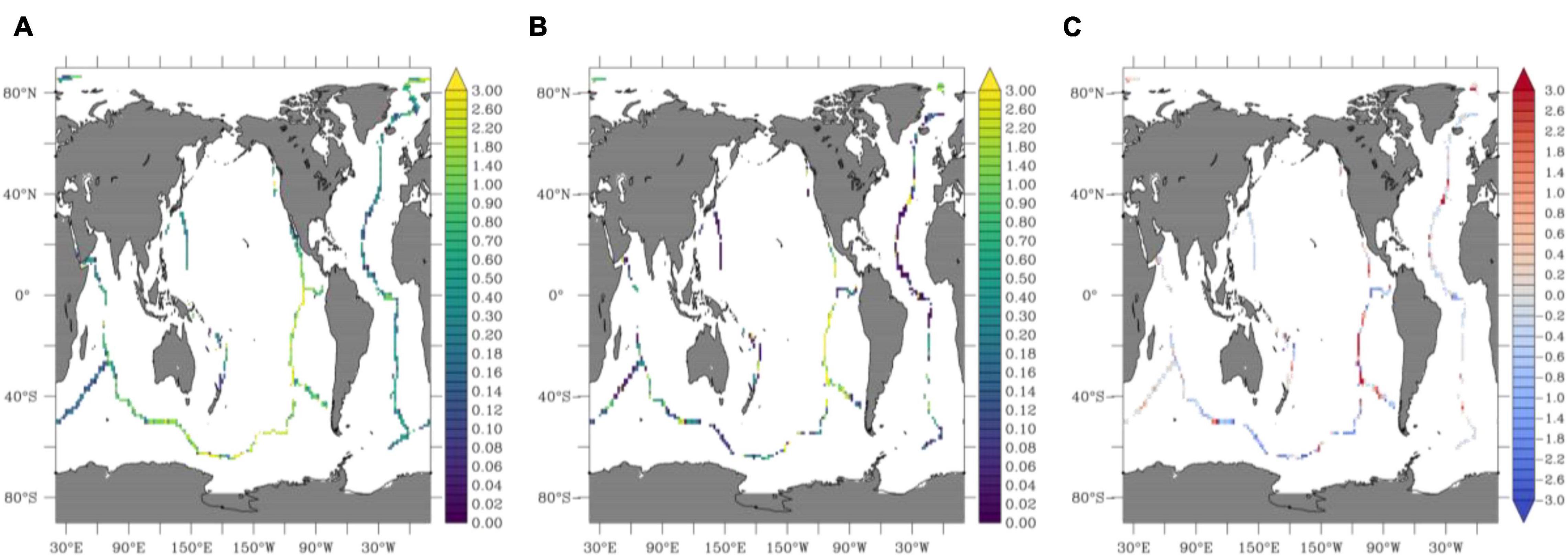
Figure 1. Hydrothermal Fe input for (A) spreading and (B) inverse hydrothermal input experiments and (C) difference between inverse and spreading experiments, all in mmol Fe m^–2 yr^–1.

Anomalies in dFe due to hydrothermal Fe are calculated by comparing the dFe field from our model under either the spreading or inverse experiments to the control simulation with no hydrothermal Fe input. Calculated in this way, full depth integrated hydrothermal Fe signals largely follow the differences in hydrothermal Fe input between the two scenarios (Figures 2A,B), with the inverse experiment exhibiting a strong increase in dFe adjacent to the SEPR and locally south of the Azores along the northern mid Atlantic ridge. Relative to the spreading input, the inverse experiment causes persistent and widespread declines elsewhere, notably along the Southern ridge systems, throughout the Indian Ocean and southern mid Atlantic Ridge (Figure 2C). Turning to the upper 200 m, the hydrothermal Fe signals that have made their way toward the ocean surface mixed layer can be isolated. Here, the overall pattern of the hydrothermal Fe anomaly is consistent between the two helium input scenarios, due to the identical circulation scheme used for these experiments and the well-known ventilation of ³He into the Southern Ocean (Figures 2D,E). However, despite having the same total hydrothermal Fe supply as the spreading experiment, spatial differences in the inverse experiment cause a 4–5 fold reduction in the contribution of hydrothermal dFe in the upper 200 m (Figure 2F). The major differences between the two scenarios is now strongly localised in the Southern Ocean, where a large fraction of the hydrothermal Fe signal has been eliminated. Similarly, the Tonga Arc and Lau basin show no hydrothermal Fe signal under the inverse experiment, in contrast to local observations (Guieu et al., 2018). The difference in strength of the Fe anomaly between the depth integrated and 0–200 m inventories for both experiments reflects the substantial losses of hydrothermal Fe in the ocean interior due to scavenging discussed in early modelling efforts (Tagliabue et al., 2010).

FIGURE 2

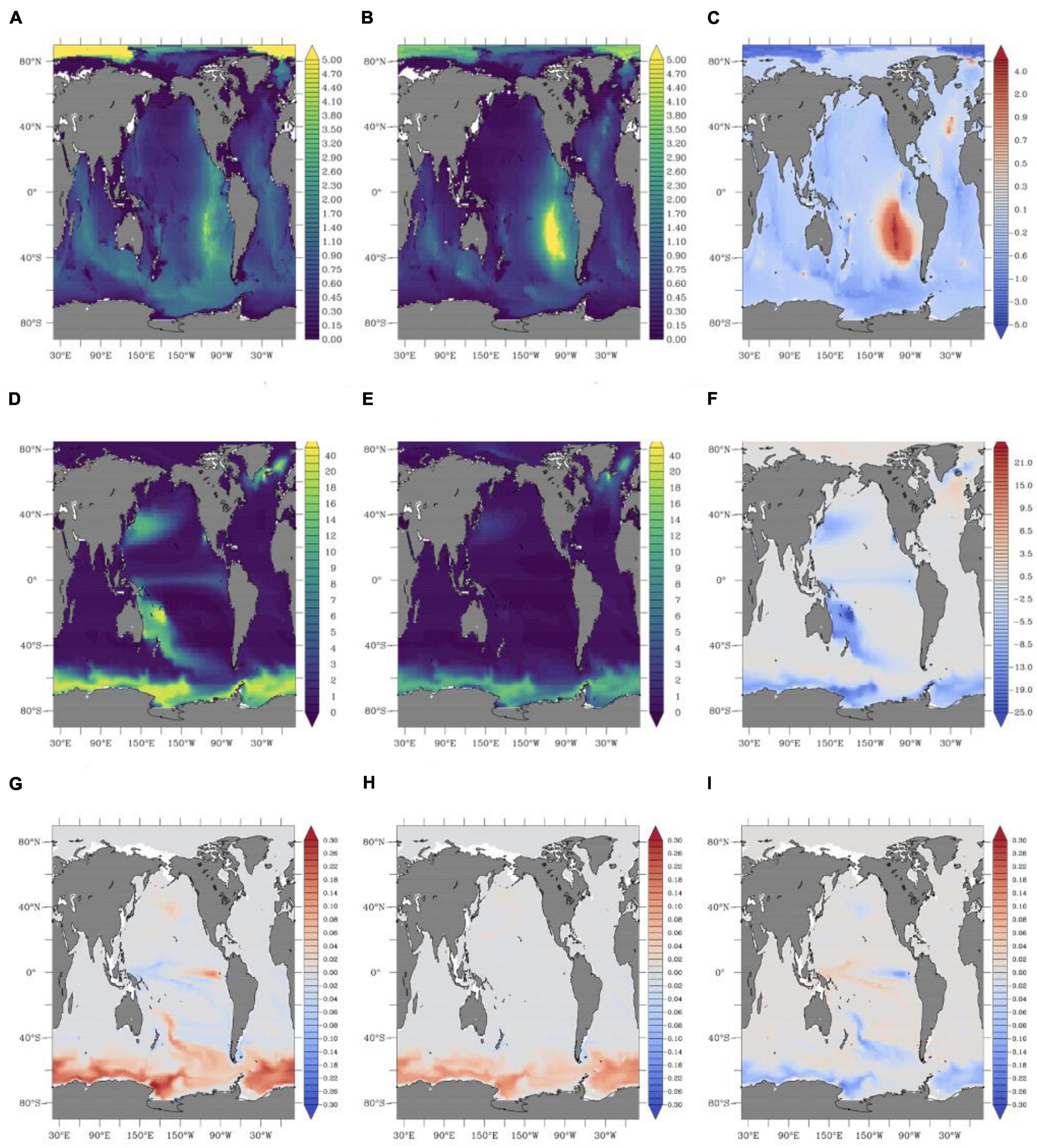
Figure 2. The impact of hydrothermal vents on the concentration of dissolved iron over the full water column (in mmol m^–2, evaluated as the difference between each experiment and the run with no hydrothermal Fe input) for (A) spreading and (B) inverse hydrothermal input experiments and (C) difference between inverse and spreading experiments, the impact of hydrothermal vents on the concentration of dissolved iron over the upper 200 m (in μmol m^–2) for (D) spreading and (E) inverse hydrothermal input and (F) difference between inverse and spreading, and the impact of hydrothermal Fe on the biological carbon pump at 100 m (mol C m^–2 yr^–1) for (G) spreading and (H) inverse hydrothermal input experiments and (I) difference between inverse and spreading.

Impact of Hydrothermal Fe Supply Scenarios on Carbon Cycling

Anomalies in export production due to hydrothermal Fe closely follow the differences in 0–200 m dFe associated with hydrothermal supply. The spreading input experiment displays positive carbon export anomalies linked to hydrothermal Fe predominantly in the Southern Ocean, but with some smaller hotspots around the Lau basin (Cohen et al., 2021), north Pacific (Jenkins et al., 2020), and equatorial Pacific regions [Figure 2G, as in previous studies (Resing et al., 2015; Tagliabue and Resing, 2016)]. Small negative anomalies in export production arise due to downstream major nutrient deficits. Under the inverse input experiment, positive carbon export anomalies are restricted only to the Southern Ocean (Figure 2H). In line with the changes in the upper 200 m dFe signals, the Southern Ocean carbon export signal associated with hydrothermal Fe declines substantially during the inverse experiment (Figure 2I).

In the spreading input experiment, hydrothermal Fe stimulates export production by 3.84 Tmol C yr^–1 south of 40°S, relative to a simulation with no hydrothermal Fe input [as in prior work (Tagliabue and Resing, 2016)]. The contribution of hydrothermal Fe is reduced by over a third (36%) to 2.45 Tmol C yr^–1 in the inverse input experiment. When changes to the spatial distribution and supply of total hydrothermal Fe supply are accounted for in the inverseR experiment, the hydrothermal iron impact on Southern Ocean export production reduces by 73%, to 1.06 Tmol C yr^–1. Thus, the redistribution of hydrothermal Fe input away from the Southern ridges in the inverse input experiment causes a significant reduction in the assumed impact of hydrothermal Fe on Southern Ocean export production that is amplified when proposed adjustments to both the spatial distribution and magnitude of Fe inputs (Roshan et al., 2020) are accounted for. Overall, despite using a different circulation model and a more complete global Fe ad C cycling model, we agree with Roshan et al. (2020) that there is negligible impact of hydrothermal Fe on the export production that supports the Southern Ocean biological carbon pump when the hydrothermal Fe input is parameterised based on ³He inverse modelling. Our experiments go further though, and also indicate that this difference is primarily due to the geographic distribution of hydrothermal Fe inputs along the global mid-ocean ridge crest, rather than being simply due to the overall magnitude of hydrothermal Fe supply between studies (as both the spreading and inverse experiments have the exact same total hydrothermal Fe supply).

Constraints on Hydrothermal Fe Supply Scenarios From Southern Ocean Observations

The inverse ³He input field has been shown to improve the reproduction of ocean ³He measurements (DeVries and Holzer, 2019), but the spatial redistribution of ³He inputs leads to the hydrothermal Fe anomaly reaching the upper ocean to be much reduced. As differences in the dFe anomalies around the circum-Antarctic ridges drive the majority of the Southern Ocean biological carbon pump signal associated with hydrothermal Fe, they provide the best observational constraints on different hydrothermal Fe input scenarios (Tagliabue and Resing, 2016). The GEOTRACES section cruise GS01 is the first full depth Southern Ocean section cruise to occupy meridional stations across the circum-Antarctic ridge between Hobart (Tasmania) and Antarctica. In the deep ocean (below 1,000 m depth), the dFe observations from the GS01 section are relatively uniform north and south of the circum-Antarctic ridge, located at around 50–55°S (Figure 3). The low deep-ocean values typical of the Southern Ocean endmember of around 0.4 nM and the slightly higher values closer to Tasmania of around 0.6 nM are similar to previous work in the region (Sedwick et al., 2008; Bowie et al., 2009). Most striking is the clear hotspot of dFe exceeding 1 nM above the circum-Antarctic ridge system that is well resolved across multiple stations and depths (Figure 3), and consistent with the observed abyssal dissolved manganese (dMn) distributions above and north and south of the ridge system (Latour et al., 2021).

FIGURE 3

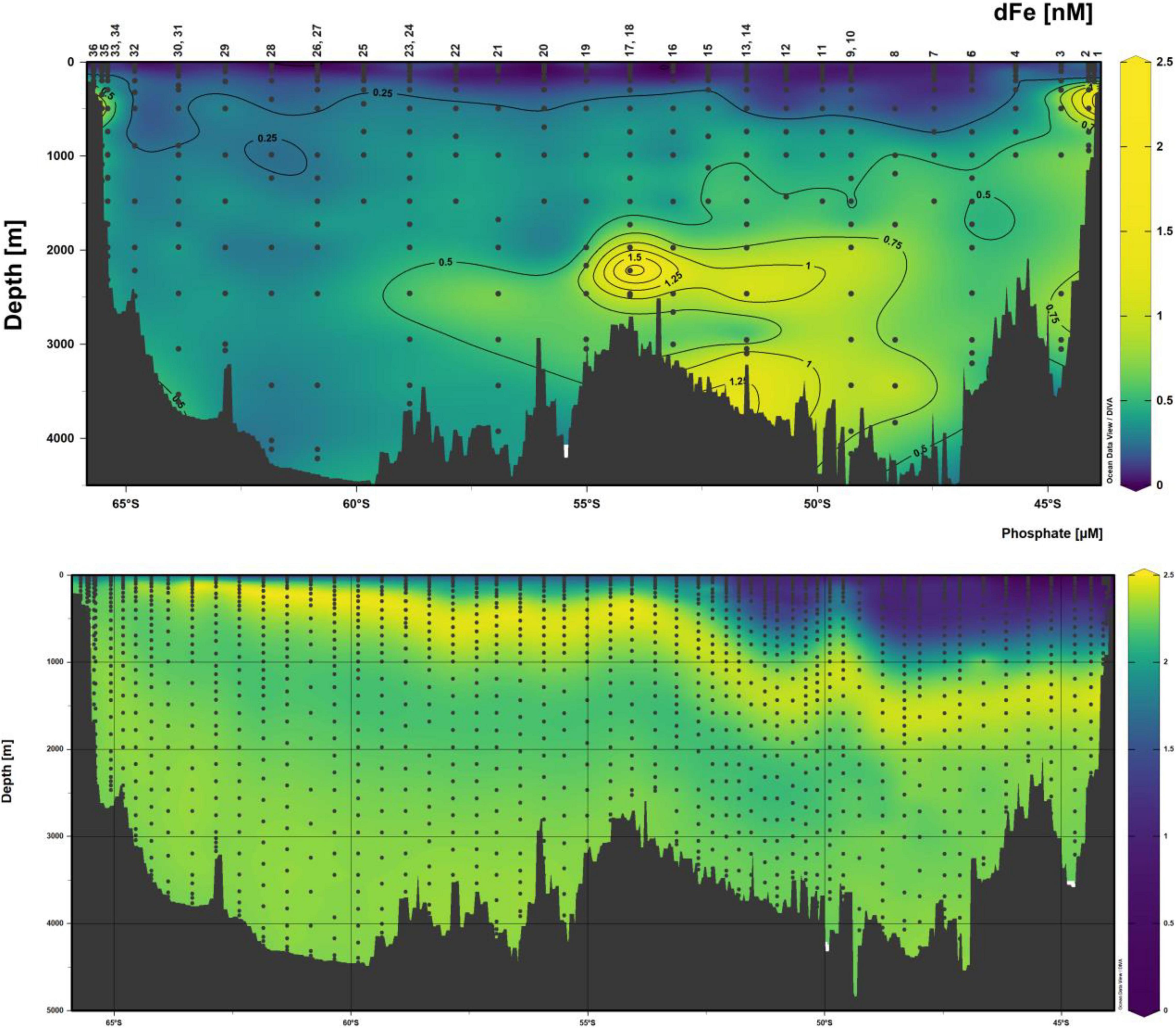
Figure 3. The distribution of dFe (nM, upper) and PO₄ (μM, lower) along the GS01 section from Antarctica (left) to Tasmania (right), highlighting the strong enrichment in dFe over the circum-Antarctic ridge between around 52 and 55°S.

Comparing the dFe fields from the spreading or inverse experiments to the available data shows that only spreading input experiment is able to reproduce the observed level of dFe enrichment above Southern Ocean ridges. We binned the GS01 observations onto the same vertical grid as the model to ensure an appropriate comparison (Figures 4A,B). In the spreading experiment, the model reproduces the hotspot of dFe over the ridge observed during GS01 (Figures 4B,C) and displays a correlation coefficient of 0.63 along the entire GS01 abyssal ocean dataset (deeper than 1,000 m, Figure 4E). In contrast, the inverse experiment produces no discernible dFe signal above the ridge (Figure 4D) and has a ∼3-fold lower correlation of 0.26 (Figure 4F). The correlation coefficient drops markedly to −0.24 in the inverseR experiment, when we apply the optimised Fe/He ratio of Roshan et al. (2020) and the spatial distribution of ³He inputs from the inverse input, indicating anti correlation between the model and observations. Without any hydrothermal Fe input, the model becomes even more strongly anti-correlated with the GS01 observations (R = −0.47), indicating the importance of significant hydrothermal Fe supply from Southern Ocean ridges in reproducing Southern Ocean dFe observations first advanced in earlier work (Tagliabue et al., 2010). Overall, this suggests that the greater impact of hydrothermal Fe on the biological carbon pump from the spreading experiment is more consistent with dFe observations.

FIGURE 4

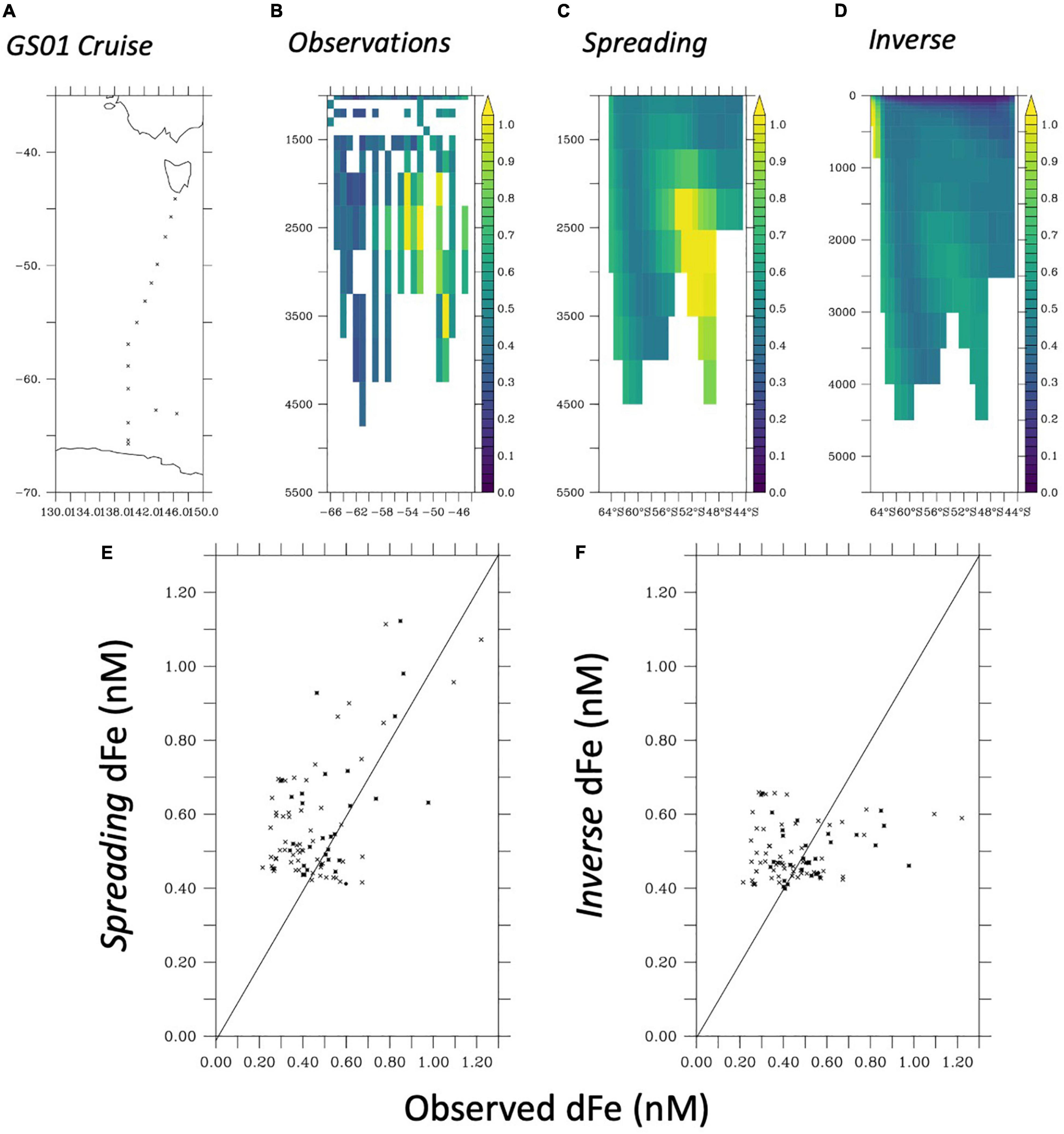
Figure 4. (A) Cruise track from GS01 section, (B) dFe observations from GS01 binned onto the model vertical axis deeper than 1,000 m, (C) modelled dFe from the spreading experiment, (D) modelled dFe from the inverse experiment. (E,F) Present a cross plot of modelled and binned observed dFe from the spreading and inverse experiments for the same model grid cells deeper than 1,000 m [the 1:1 line is marked in black for (E,F)].

What Is the Residence Time for Hydrothermal Fe?

The residence time of hydrothermal Fe, relative to its ultimate removal by scavenging, is a key component governing its longevity and potential surface water ventilation. Observations from the GP16 section in the east Pacific using different tracers suggest that the hydrothermal iron emitted from the southern East Pacific Rise had a residence time of a few tens of years (Kipp et al., 2018; Anderson, 2020). This is lower than that implied from the quasi-conservative behaviour of iron, with respect to helium, observed during the 50–75 years transport of waters westward from the ridge crest (Resing et al., 2015; Fitzsimmons et al., 2017). Iron cycle modelling based solely on representing a pool of hydrothermal Fe and the inverse Fe boundary forcing suggests that the residence time of hydrothermal Fe was 30 ± 10 years, implying little opportunity for surface ventilation (Roshan et al., 2020). In our modelling exercise, we can derive the residence time for hydrothermal Fe, relative to removal by scavenging, using the dFe anomaly with respect to the simulation with no hydrothermal Fe supply and the magnitude of the hydrothermal dFe boundary forcing appropriate for each experiment. The total hydrothermal iron inventory south of 55°S is 25 and 12 Gmol Fe (for the spreading and inverse experiments, respectively) or 250 and 210 Gmol Fe globally (for the spreading and inverse experiments, respectively). The companion Fe inputs are 1.1 and 0.4 Gmol Fe yr^–1 in the Southern Ocean (for the spreading and inverse experiments, respectively) and 10 Gmol yr^–1 globally for both scenarios. This results in hydrothermal Fe residence times of 22 and 34 years in the Southern Ocean (for the spreading and inverse inputs, respectively) or 25 and 21 years globally (for the spreading and inverse inputs, respectively). In our model, dFe gets stabilised due to interactions with ligands, alongside colloidal and scavenging interactions with the particle pool. The residence times derived are at the lower end of those previously proposed, yet we find hydrothermal Fe maintains a strong contribution to the export production that drives the Southern Ocean biological carbon pump. These results re-affirm the importance of Southern Ocean ridges (Tagliabue and Resing, 2016) as the critical factor governing hydrothermal Fe impacts on the carbon cycle, since only they can ventilate iron on sufficiently rapid timescales before hydrothermal Fe is removed by scavenging. Finally, our findings suggest that while hydrothermal vents outside of surface ventilation and mixing hotspots are important for the interior ocean Fe cycle, they are unlikely to affect the upper ocean significantly (unless they are present at shallow depths).

Wider Implications

Our findings suggest that trapping of Fe in the ocean interior by reversible scavenging is of secondary importance to the geographic distribution of hydrothermal Fe supply, relative to ocean mixing regimes, in regulating the impact on the carbon cycle. Until now, modelling efforts have focussed on mid ocean ridge spreading systems in the Southern Ocean (e.g., Figures 1A,B), which neglects other sites of hydrothermal activity and iron supply. For instance, the Scotia Sea in the south Atlantic hosts a range of back arc and arc volcano sites that are notable iron sources (Hawkes et al., 2013, 2014) but are not yet accounted for in Fe cycle modelling efforts. Similarly, in the Indian sector, shallow venting from the active volcanoes around the Heard and McDonald Islands supplies Fe (Holmes et al., 2020) further south than the mid ocean ridge system. Finally, hydrothermal sites in the Bransfield Strait have been discovered (Klinkhammer et al., 2001), with Fe supply from the hydrothermal sediments inferred (Aquilina et al., 2014). It is clear that updated model hydrothermal sources above and beyond those associated with mid-ocean ridges and moving beyond simple linkages with He will be important in addressing regional impacts on Fe cycling, especially in the Atlantic sector of the Southern Ocean.

While our ability to represent hydrothermal Fe will be helped by more complete datasets concerning inputs, the impact on the Southern Ocean carbon cycle requires a more holistic consideration. Hydrothermal vents are not the only Fe source in the region, with important roles for margin sediments, sea ice, icebergs and melting glaciers, as well as aeolian deposition (from South America, Australia and southern Africa, alongside the dry valleys further south) (Boyd and Ellwood, 2010; Bhattachan et al., 2015; Tagliabue et al., 2017). The role for hydrothermal Fe operates alongside these other sources, which can end up amplifying or dampening the carbon cycle impact in model assessments where the full range of iron sources are represented (Tagliabue et al., 2010). Spatially, hydrothermal supply is focussed on regions of deep water ventilation in the Antarctic sector (Figure 2), which overlaps most with sources associated with melting sea ice and transport of margin Fe from the Antarctic continental shelf (Boyd et al., 2012). This “Fe supply” mosaic will be important in attributing measured dFe signals to hydrothermalism (Schine et al., 2021). Progress on the Fe supply from hydrothermal vents alone will still leave outstanding questions regarding Fe supply from other sources.

The effective impact of Fe from Southern Ocean hydrothermal vents is regulated by the physical processes shaping the distribution, magnitude and timescales for deep ocean ventilation. Our study suggests that the residence time for hydrothermal Fe is on the order of a few tens of years, which requires upper ocean ventilation to be sufficiently rapid. The conservative hydrothermal tracer ³He has been estimated to emerge in Southern Ocean surface waters within 99 ± 18 years (Jenkins, 2020), similar to the median re-exposure timescale from the deep Southern Ocean calculated from data constrained ocean physical models (DeVries and Holzer, 2019; Weber, 2020). Estimates from particle tracking models at higher spatial resolution suggest more rapid ventilation timescales of around 20 years, which slow to many decades in coarser resolution configurations (Tamsitt et al., 2017; Drake et al., 2018). Overall, ventilation timescales on the order of a few decades are compatible with a relatively short residence time for hydrothermal Fe. Ventilation of ridge associated signals may also be assisted if the topographic interaction promotes diapycnal transfer onto lighter isopycnals, which will then ventilate more rapidly (Sokolov and Rintoul, 2007). More focussed work on ocean mixing around Southern Ocean ridge systems over different space scales, alongside more process-based constraints on the rates and timescales of Fe removal, are necessary for improved insight.

Conclusion

Combining ocean model experiments with new observations of dFe from the deep Southern Ocean, we find that the hydrothermal supply of Fe in the Southern Ocean is not well constrained by the spatial distribution of ³He inputs. This supports an important role of hydrothermal Fe in shaping upper ocean biological activity and export production in the Southern Ocean and the regional biological carbon pump. Due to the primary role played by hydrothermal Fe input along Southern Ocean ridges, the residence time of a few tens of years for hydrothermal Fe, relative to scavenging removal, estimated here is compatible with the expected physical mixing timescales in the region. Future work that expands the representation of hydrothermal activity in the Southern Ocean beyond the mid ocean ridges will be important for refining ocean modelling and the carbon cycle impact. Expanded observational constraints on how the distribution and timescales of ocean physical mixing interface with ocean Fe cycling around Southern Ocean ridges will help develop more robust assessments of the fate and impact of hydrothermal Fe on the carbon cycle.

Data Availability Statement

The datasets presented in this study can be found in online repositories. The names of the repository/repositories and accession number(s) can be found below: https://doi.org/10.5281/zenodo.5507411.

Author Contributions

AT was designed the study, conducted all model experiments and their analysis, and led the writing of the manuscript with input from AB and JR. AB led the collection of dissolved iron data from the Southern Ocean. TH, PL, PM, MG-R, and KW participated in sample collection and analysis. All authors commented on the final draft and revisions.

Funding

AT was supported by funding from NERC (NE/N009525/1). AB was supported by the Antarctic Climate and Ecosystems Cooperative Research Centre (ACE CRC) and Australian Research Council through the Future Fellowships Program (FT130100037). JR was funded by NOAA Earth-Ocean Interactions Program and Office of Ocean Exploration and Research and United States National Science Foundation OCE1756402.

Conflict of Interest

The authors declare that the research was conducted in the absence of any commercial or financial relationships that could be construed as a potential conflict of interest.

Publisher’s Note

All claims expressed in this article are solely those of the authors and do not necessarily represent those of their affiliated organizations, or those of the publisher, the editors and the reviewers. Any product that may be evaluated in this article, or claim that may be made by its manufacturer, is not guaranteed or endorsed by the publisher.

Acknowledgments

We thank three reviewers for their comments that improved the manuscript. We also thank Tim DeVries (UCSB) for supplying the OCIM inverse model helium-3 input field. We wish to acknowledge the crew and officers of the Australian Marine National Facility Vessel RV Investigator for support at sea during the 2018 SR3 voyage (GS01) and also Morgane Perron, Christine Weldrick, Matthew Corkill, and Ashley Townsend for assisting with the sampling and sample processing. Data associated with this publication is available at: https://doi.org/10.5281/zenodo.5507411. This is PMEL contribution number 5293 and JISAO publication contribution 2021-1156.

References

Anderson, R. F. (2020). GEOTRACES: Accelerating Research on the Marine Biogeochemical Cycles of Trace Elements and Their Isotopes. Ann. Rev. Mar. Sci. 12, 49–85. doi: 10.1146/annurev-marine-010318-095123

PubMed Abstract | CrossRef Full Text | Google Scholar

Aquilina, A., Homoky, W. B., Hawkes, J. A., Lyons, T. W., and Mills, R. A. (2014). Hydrothermal sediments are a source of water column Fe and Mn in the Bransfield Strait, Antarctica. Geochimica et Cosmochimica Acta 137, 64–80. doi: 10.1016/j.gca.2014.04.003

CrossRef Full Text | Google Scholar

Ardyna, M., Lacour, L., Sergi, S., D’ovidio, F., Sallee, J. B., Rembauville, M., et al. (2019). Hydrothermal vents trigger massive phytoplankton blooms in the Southern Ocean. Nat. Commun. 10:2451. doi: 10.1038/s41467-019-09973-6

PubMed Abstract | CrossRef Full Text | Google Scholar

Aumont, O., Ethé, C., Tagliabue, A., Bopp, L., and Gehlen, M. (2015). PISCES-v2: an ocean biogeochemical model for carbon and ecosystem studies. Geosci. Mod. Develop. 8, 2465–2513. doi: 10.5194/gmd-8-2465-2015

CrossRef Full Text | Google Scholar

Bhattachan, A., Wang, L., Miller, M. F., Licht, K. J., and D’odorico, P. (2015). Antarctica’s Dry Valleys: a potential source of soluble iron to the Southern Ocean? Geophys. Res. Lett. 42, 1912–1918. doi: 10.1002/2015gl063419

CrossRef Full Text | Google Scholar

Bianchi, D., Sarmiento, J. L., Gnanadesikan, A., Key, R. M., Schlosser, P., and Newton, R. (2010). Low helium flux from the mantle inferred from simulations of oceanic helium isotope data. Earth Planet. Sci. Lett. 297, 379–386.

Google Scholar

Bowie, A. R., Lannuzel, D., Remenyi, T. A., Wagener, T., Lam, P. J., Boyd, P. W., et al. (2009). Biogeochemical iron budgets of the Southern Ocean south of Australia: decoupling of iron and nutrient cycles in the subantarctic zone by the summertime supply. Glob. Biogeochem. Cyc. 23:4034.

Google Scholar

Boyd, P. W., Arrigo, K. R., Strzepek, R., and Van Dijken, G. L. (2012). Mapping phytoplankton iron utilization: Insights into Southern Ocean supply mechanisms. J. Geophys. Res. 117:C06009.

Google Scholar

Boyd, P. W., and Ellwood, M. J. (2010). The biogeochemical cycle of iron in the ocean. Nat. Geosci. 3, 675–682.

Google Scholar

Cohen, N. R., Noble, A. E., Moran, D. M., Mcilvin, M. R., Goepfert, T. J., Hawco, N. J., et al. (2021). Hydrothermal trace metal release and microbial metabolism in the northeastern Lau Basin of the South Pacific Ocean. Biogeosciences 18, 5397–5422.

Google Scholar

DeVries, T., and Holzer, M. (2019). Radiocarbon and Helium Isotope Constraints on Deep Ocean Ventilation and Mantle 3-He Sources. J. Geophys. Res. Oceans 124, 3036–3057. doi: 10.1029/2018jc014716

CrossRef Full Text | Google Scholar

Drake, H. F., Morrison, A. K., Griffies, S. M., Sarmiento, J. L., Weijer, W., and Gray, A. R. (2018). Lagrangian Timescales of Southern Ocean Upwelling in a Hierarchy of Model Resolutions. Geophys. Res. Lett. 45, 891–898. doi: 10.1002/2017gl076045

CrossRef Full Text | Google Scholar

Dutay, J. C., Jean-Baptiste, P., Campin, J. M., Ishida, A., Maier-Reimer, E., Matear, R. J., et al. (2004). Evaluation of OCMIP-2 ocean models’ deep circulation with mantle helium-3. J. Mar. Sys. 48, 15–36.

Google Scholar

Farley, K. A., Maier-Reimer, E., Schlosser, P., and Broecker, W. S. (1995). Constraints on mantle3He fluxes and deep-sea circulation from an oceanic general circulation model. J. Geophys. Res.: Solid Earth 100, 3829–3839. doi: 10.1029/94jb02913

CrossRef Full Text | Google Scholar

Fitzsimmons, J. N., John, S. G., Marsay, C. M., Hoffman, C. L., German, C. R., and Sherrell, R. M. (2017). Iron persistence in a distal hydrothermal plume supported by dissolved–particulate exchange. Nat. Geosci. 10, 195–201. doi: 10.1038/ngeo2900

CrossRef Full Text | Google Scholar

German, C. R., Casciotti, K. A., Dutay, J. C., Heimbürger, L. E., Jenkins, W. J., Measures, C. I., et al. (2016). Hydrothermal impacts on trace element and isotope ocean biogeochemistry. Philosophical Transactions of the Royal Society. : Math. Phys. Eng. Sci. 374:20160035. doi: 10.1098/rsta.2016.0035

PubMed Abstract | CrossRef Full Text | Google Scholar

Guieu, C., Bonnet, S., Petrenko, A., Menkes, C., Chavagnac, V., Desboeufs, K., et al. (2018). Iron from a submarine source impacts the productive layer of the Western Tropical South Pacific (WTSP). Sci. Rep. 8:9075. doi: 10.1038/s41598-018-27407-z

PubMed Abstract | CrossRef Full Text | Google Scholar

Hatta, M., Measures, C. I., Wu, J., Roshan, S., Fitzsimmons, J. N., Sedwick, P., et al. (2015). An overview of dissolved Fe and Mn distributions during the 2010–2011 U.S. Top. Stud. Oceanogr. 116, 117–129.

Google Scholar

Hawkes, J. A., Connelly, D. P., Gledhill, M., and Achterberg, E. P. (2013). The stabilisation and transportation of dissolved iron from high temperature hydrothermal vent systems. Earth Planet. Sci. Lett. 375, 280–290. doi: 10.1016/j.epsl.2013.05.047

CrossRef Full Text | Google Scholar

Hawkes, J. A., Connelly, D. P., Rijkenberg, M. J. A., and Achterberg, E. P. (2014). The importance of shallow hydrothermal island arc systems in ocean biogeochemistry. Geophys. Res. Lett. 41, 942–947. doi: 10.1073/pnas.2019021117

PubMed Abstract | CrossRef Full Text | Google Scholar

Holmes, T. M., Wuttig, K., Chase, Z., Schallenberg, C., Merwe, P., Townsend, A. T., et al. (2020). Glacial and Hydrothermal Sources of Dissolved Iron (II) in Southern Ocean Waters Surrounding Heard and McDonald Islands. J. Geophys. Res. Oceans 125:e2020JC016286.

Google Scholar

Holzer, M., Devries, T., Bianchi, D., Newton, R., Schlosser, P., and Winckler, G. (2017). Objective estimates of mantle 3He in the ocean and implications for constraining the deep ocean circulation. Earth Planet. Sci. Lett. 458, 305–314. doi: 10.1016/j.epsl.2016.10.054

CrossRef Full Text | Google Scholar

Jenkins, W. J. (2020). Using Excess 3-He to Estimate Southern Ocean Upwelling Time Scales. Geophys. Res. Lett. 47, e2020GL087266.

Google Scholar

Jenkins, W. J., Hatta, M., Fitzsimmons, J. N., Schlitzer, R., Lanning, N. T., Shiller, A., et al. (2020). An intermediate-depth source of hydrothermal 3He and dissolved iron in the North Pacific. Earth Planet. Sci. Lett. 539:116223.

Google Scholar

Jenkins, W. J., Lott, D. E., German, C. R., Cahill, K. L., Goudreau, J., and Longworth, B. (2018). The deep distributions of helium isotopes, radiocarbon, and noble gases along the U.S. GEOTRACES East Pacific Zonal Transect (GP16). Mar. Chem. 201, 167–182. doi: 10.1016/j.marchem.2017.03.009

CrossRef Full Text | Google Scholar

Jenkins, W. J., Lott, D. E., Longworth, B. E., Curtice, J. M., and Cahill, K. L. (2015). The distributions of helium isotopes and tritium along the U.S. GEOTRACES North Atlantic sections (GEOTRACES GAO3). Deep Sea Res. Part II Top. Stud. Oceanogr. 116, 21–28.

Google Scholar

Kipp, L. E., Sanial, V., Henderson, P. B., Van Beek, P., Reyss, J.-L., Hammond, D. E., et al. (2018). Radium isotopes as tracers of hydrothermal inputs and neutrally buoyant plume dynamics in the deep ocean. Mar. Chem. 201, 51–65. doi: 10.1016/j.marchem.2017.06.011

CrossRef Full Text | Google Scholar

Klinkhammer, G. P., Chin, C. S., Keller, R. A., Dählmann, A., Sahling, H., Sarthou, G., et al. (2001). Discovery of new hydrothermal vent sites in Bransfield Strait, Antarctica. Earth Planet. Sci. Lett. 193, 395–407. doi: 10.1016/s0012-821x(01)00536-2

CrossRef Full Text | Google Scholar

Klunder, M. B., Bauch, D., Laan, P., De Baar, H. J. W., Van Heuven, S., and Ober, S. (2012). Dissolved iron in the Arctic shelf seas and surface waters of the central Arctic Ocean: Impact of Arctic river water and ice-melt. J. Geophys. Res.Oceans 117:18.

Google Scholar

Klunder, M. B., Laan, P., Middag, R., De Baar, H. J. W., and Van Ooijen, J. C. (2011). Dissolved iron in the Southern Ocean (Atlantic sector). Deep Sea Research Part II. Top. Stud. Oceanogr. 58, 2678–2694. doi: 10.1016/j.dsr2.2010.10.042

CrossRef Full Text | Google Scholar

Latour, P., Wuttig, K., Van, Der Merwe, Holmes, T. M., Corkill, M., and Bowie, A. R. (2021). Manganese biogeochemistry in the Southern Ocean, from Tasmania to Antarctica. Limnol. Oceanogr. 66, 2547–2562.

Google Scholar

Nishioka, J., Obata, H., and Tsumune, D. (2013). Evidence of an extensive spread of hydrothermal dissolved iron in the Indian Ocean. Earth Planet. Sci. Lett. 361, 26–33.

Google Scholar

Resing, J. A., Sedwick, P. N., German, C. R., Jenkins, W. J., Moffett, J. W., Sohst, B. M., et al. (2015). Basin-scale transport of hydrothermal dissolved metals across the South Pacific Ocean. Nature 523, 200–203. doi: 10.1038/nature14577

PubMed Abstract | CrossRef Full Text | Google Scholar

Rijkenberg, M. J., Middag, R., Laan, P., Gerringa, L. J., Van Aken, H. M., Schoemann, V., et al. (2014). The distribution of dissolved iron in the West Atlantic Ocean. PLoS One 9:e101323. doi: 10.1371/journal.pone.0101323

PubMed Abstract | CrossRef Full Text | Google Scholar

Roshan, S., Devries, T., Wu, J., John, S., and Weber, T. (2020). Reversible scavenging traps hydrothermal iron in the deep ocean. Earth Planet. Sci. Lett. 542:116297. doi: 10.1016/j.epsl.2020.116297

CrossRef Full Text | Google Scholar

Saito, M. A., Noble, A. E., Tagliabue, A., Goepfert, T. J., Lamborg, C. H., and Jenkins, W. J. (2013). Slow-spreading submarine ridges in the South Atlantic as a significant oceanic iron source. Nat. Geosci. 6, 775–779.

Google Scholar

Schine, C. M. S., Alderkamp, A. C., Van Dijken, G., Gerringa, L. J. A., Sergi, S., Laan, P., et al. (2021). Massive Southern Ocean phytoplankton bloom fed by iron of possible hydrothermal origin. Nat. Commun. 12:1211. doi: 10.1038/s41467-021-21339-5

PubMed Abstract | CrossRef Full Text | Google Scholar

Schlitzer, R., Anderson, R. F., Dodas, E. M., Lohan, M., Geibert, W., Tagliabue, A., et al. (2018). The GEOTRACES Intermediate Data Product 2017. Chem. Geol. 493, 210–223. doi: 10.1073/pnas.1603107114

PubMed Abstract | CrossRef Full Text | Google Scholar

Sedwick, P. N., Bowie, A. R., and Trull, T. W. (2008). Dissolved iron in the Australian sector of the Southern Ocean (CLIVAR SR3 section): meridional and seasonal trends. Oceanogr. Res. Pap. 55, 911–925. doi: 10.1016/j.dsr.2008.03.011

CrossRef Full Text | Google Scholar

Sokolov, S., and Rintoul, S. R. (2007). On the relationship between fronts of the Antarctic Circumpolar Current and surface chlorophyll concentrations in the Southern Ocean. J. Geophys. Res. 112:7030. doi: 10.1029/2006JC004072

CrossRef Full Text | Google Scholar

Tagliabue, A., Bopp, L., Dutay, J. C., Bowie, A. R., Chever, F., Jean-Baptiste, P., et al. (2010). Hydrothermal contribution to the oceanic dissolved iron inventory. Nat. Geosci. 3, 252–256.

Google Scholar

Tagliabue, A., Bowie, A. R., Boyd, P. W., Buck, K. N., Johnson, K. S., and Saito, M. A. (2017). The integral role of iron in ocean biogeochemistry. Nature 543, 51–59. doi: 10.1038/nature21058

PubMed Abstract | CrossRef Full Text | Google Scholar

Tagliabue, A., and Resing, J. (2016). Impact of hydrothermalism on the ocean iron cycle. Philos. Trans. Math. Phys. Eng. Sci. 374:20150291. doi: 10.1098/rsta.2015.0291

PubMed Abstract | CrossRef Full Text | Google Scholar

Tamsitt, V., Drake, H. F., Morrison, A. K., Talley, L. D., Dufour, C. O., Gray, A. R., et al. (2017). Spiraling pathways of global deep waters to the surface of the Southern Ocean. Nat. Commun. 8:172.

Google Scholar

Völker, C., and Tagliabue, A. (2015). Modeling organic iron-binding ligands in a three-dimensional biogeochemical ocean model. Mar. Chem. 173, 67–77.

Google Scholar

Weber, T. (2020). Southern Ocean Upwelling and the Marine Iron Cycle. Geophys. Res. Lett. 47:e2020GL090737.

Google Scholar

Wuttig, K., Townsend, A. T., Van Der Merwe, P., Gault-Ringold, M., Holmes, T., Schallenberg, C., et al. (2019). Critical evaluation of a seaFAST system for the analysis of trace metals in marine samples. Talanta 197, 653–668. doi: 10.1016/j.talanta.2019.01.047

PubMed Abstract | CrossRef Full Text | Google Scholar