 Juntian Chen1,2
 Xiao-Hua Zhu
 Hua Zheng
- 1Ocean College, Zhejiang University, Zhoushan, China
- 2State Key Laboratory of Satellite Ocean Environment Dynamics, Second Institute of Oceanography, Ministry of Natural Resources, Hangzhou, China
- 3Southern Marine Science and Engineering Guangdong Laboratory (Zhuhai), Zhuhai, China
- 4School of Oceanography, Shanghai Jiao Tong University, Shanghai, China
Submesoscale processes in the ocean are vital for sustaining energy balance across scales. Taking advantage of the high resolution and wide coverage of numerical simulations, which are currently lacking for field observations, we investigated the basic patterns of submesoscale dynamics and mechanisms of corresponding variabilities along with the Kuroshio in the East China Sea. The large-scale western boundary jet serves as a remarkable submesoscale energy reservoir, promoted by steep topographic features. In the discovered hotspots, that is, the continental slope and lee area of the Tokara Strait, long-lasting submesoscale footprints arose in the form of linear patterns of strongly skewed Rossby numbers with maximum values of ~O(1). Their origin may be derived from the high topographically induced strain rate, which shows a consistent distribution and high correlation with the Rossby number. Corresponding to the characteristics of such active submesoscale processes, kinetic energy wavenumber spectra were visibly flatter than previous estimations of typical two-dimensional geostrophic turbulence and were not temporally fixed under the combined effects of multiple factors. The annual cycle of stratification induces seasonality by affecting mixed-layer instabilities, which control the kinetic and potential energy conversion rates. The tidal periods may be due to tides generating inertia-gravity waves that partially overlap in submesoscale ranges. Various other intermediate periods of variability were probably related to the eddy-caused Kuroshio path meander, which implied a closely coupled dynamical system across scales. Uncertainties come from the ascertainment of the specific contribution ratios of each part, which will be studied in the future.
1. Introduction
As a continuum formed by fluids, the ocean permits the existence of wide-range spatial-length scales. It remains unclear whether the oceanic energy cascades are multi-stage processes (Davidson, 2015) and how many stages may occur, such as the electronic energy levels. It is certain that multi-scale interactions and cross-scale energy transfers exist (Qiu et al., 2022). For the large/basin-scale ocean general circulations, equilibrium is the result of energy conservation. It must be subjected to constant forcings, such as wind or solar heat flux. Eventual dissipation with turbulence at small scales (McWilliams, 2016) is also essential as an energy sink. Intermediate processes refer to forward cascades in achieving the abovementioned transfer across scales, which are usually completed through routes associated with the motions in submesoscale ranges (fronts, filaments, inertia-gravity waves, etc.). The recently discovered mechanism pointed out that the near-inertial waves, which share part of the submesoscale regime (Alford et al., 2016), can promote forward energy cascades even without participating in the processes directly (i.e., without undergoing energy change themselves). This catalytic effect (Xie, 2020) further reflects the important dynamical meaning of submesoscale motions for oceanic energetics.
Reasoning can deduce that the submesoscale energy magnitude should be coupled with that of the larger scale to a certain extent because it has redundant energy absorbed from external systems to digest. As a result, in regions where the robust western boundary currents flow, we may capture more remarkable features of the submesoscale than in places where dynamical activities are relatively moderate. It is easy to examine, as is this fact. Long-distance shipboard observation results traversing distinct dynamical regimes (Qiu et al., 2017) revealed that the energy at scales of ~200 km in the Kuroshio was approximately twice as high as in the Subtropical Countercurrent. This ratio is similar to that at a scale of ~20 km. Notably, this reasoning requires that the two compared dynamic regimes have similar power laws (for example, both being the k−3 law, where k is the wavenumber). This may give us an easily available metric to judge where a latent submesoscale energy reservoir is, given that the present relevant observations remain difficult and rare.
Except for the robust inherent energy level, extreme topographic features (such as steep shelf) make the western boundary regions ideal for the generation of submesoscale motions. Topographic features can either directly drag against or create friction with the circulations (Gula et al., 2015; Gula et al., 2016), enhance shear instability, generate submesoscale motions, or control the circulation to increase mesoscale strain (Rosso et al., 2015), which then generates submesoscale activities. In the East China Sea (ECS), the Kuroshio is not only squeezed by the long continental slope when entering but also continuously impinges against a series of islands when leaving. Therefore, typical submesoscale characteristics can be expected. This leads to a framework that depicts coupling systems across different scales that are currently inadequately understood. In addition to maintaining the energy balance of the ocean, submesoscale motions are also of significant in promoting oceanic and air–sea biochemical material exchanges, such as convergence of primary production (Zhang and Qiu, 2020), modification of water mass (Ruan et al., 2017), nutrient fluxes (Klein and Lapeyre, 2009), and carbon dioxide flux (Pezzi et al., 2021), and thus merit further attention.
This purpose of this study was to look into the submesoscale characteristics of the Kuroshio, ECS, as well as their relationships. Using long-term and high-resolution simulations, introduced in Section 2, the basic pattern and corresponding origin are presented in Section 3. A discussion of the temporal variabilities of submesoscale dynamics is presented in Section 4. The main conclusion is summarized in Section 5.
2. Data and methods
2.1. Numerical simulations
Using a relatively high-resolution reanalysis of the current dataset produced by the tide-resolving general circulation numerical model system, JCOPE-T, we obtained a glimpse into the submesoscale dynamics in the ECS. The JCOPE-T was based on one of the world community models, the Princeton Ocean Model (Varlamov et al., 2015), and was developed by the Japan Agency for Marine-Earth Science and Technology (JAMSTEC), assimilating massive in-situ observations. The model data used in this study ranged from 24°N to 32°N and from 125°E to 132°E, covering the Kuroshio region in the ECS (Figures 1C, E). Vertically, the model was divided into 47 levels that covered the entire depth range. Horizontally, ~3-km (1/36°) resolution is available for investigating submesoscale processes. The JCOPE-T dataset has been verified to accurately reproduce the circulation conditions (Liu et al., 2019) and tidal currents (Varlamov et al., 2015). In this study, tidal constituents in the dataset were removed from the raw current field. This reanalysis dataset, spanning from January 2003 to March 2012, provided the current velocity, water temperature, and salinity. Notably, the low temporal-resolution (daily) data we used are insufficient for distinguishing submesoscale currents and inertial gravity waves (IGWs), which also share the submesoscale bands.
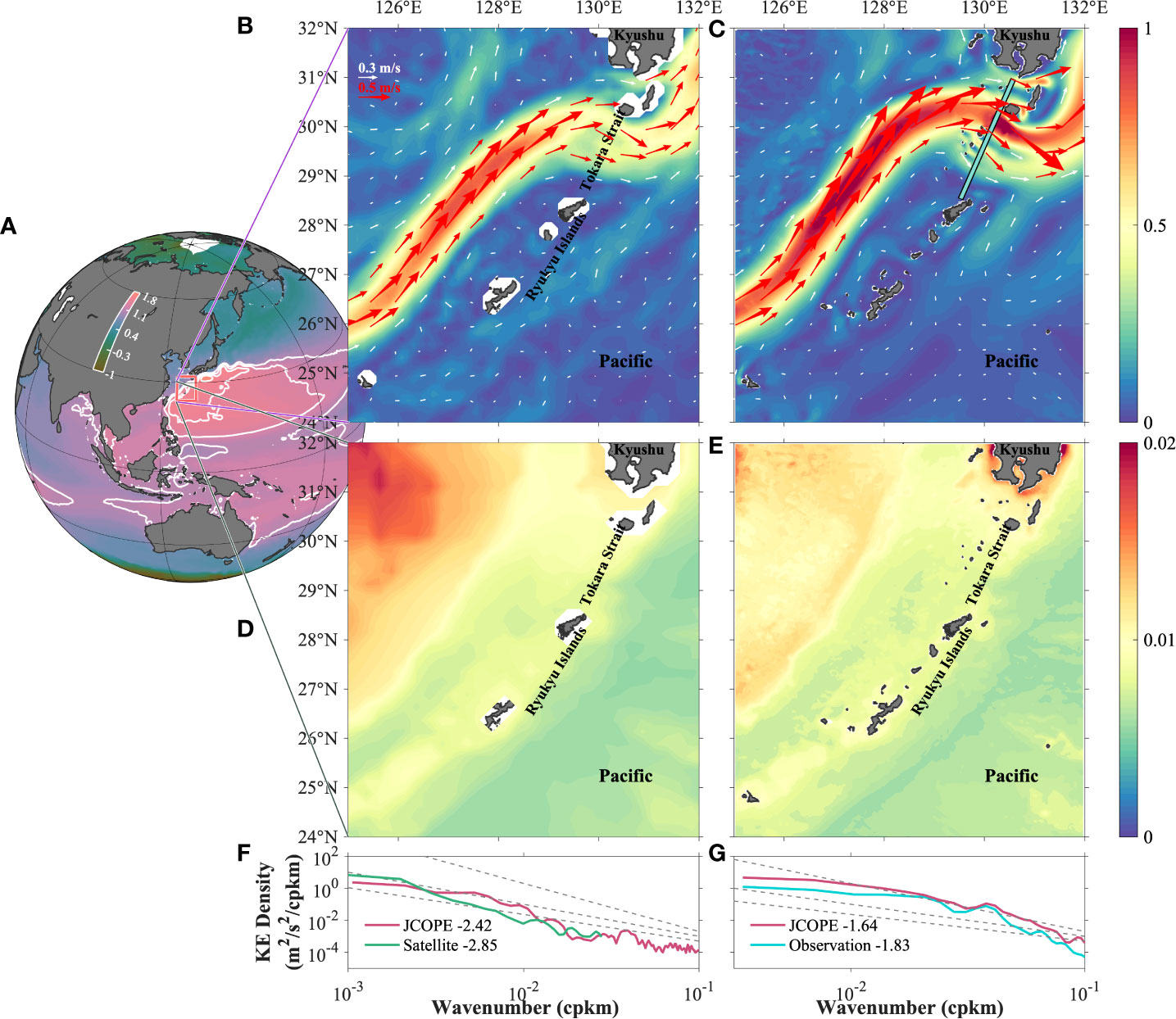
Figure 1 Basic patterns of the study area and comparison between simulations and observations. (A) A global map and climatological mean dynamic topography (MDT, unit: m). White isolines indicate MDT with an interval of 0.2 m, for a range of 1.0–1.8 m. (B) Satellites climatological and (C) JCOPE-T surface current fields (vectors) of the study area. The model results have been averaged from 2003 to 2012. Base colors represent current velocities (unit: m/s). Vectors with magnitudes greater (lesser) than 0.5 m/s are shown in red (purple). The cyan thick line in (C) is the shipboard observation track in the Tokara Strait (TkS). (D) Climatological depth-averaged buoyancy frequency (unit: s−2) from the World Ocean Atlas (WOA) climatological mean thermohaline dataset. (E) The same as (D) but from JCOPE-T simulations. (F) Surface kinetic energy wavenumber spectra along the Kuroshio axis (with the largest current velocity). The spectra were also calculated using climatological mean data. (G) Upper-layer (above 200 m) kinetic energy wavenumber spectra across the Kuroshio mainstream in the TkS (cyan line in (C)). Linear-fitted spectral slopes were numbered in (F, G). The power laws of k−5/3, k−2, and k−3 were drawn using gray dashed lines in (F, G).
2.2. Shipboard and satellite observations
To validate the JCOPE-T dataset and demonstrate that the model can resolve the submesoscale dynamics well, shipboard and satellite observation data were used for comparison.
For a region probably characterized by submesoscale processes, the Tokara Strait (TkS), long-term (January 2003–March 2012) repeated current observations were conducted by a shipboard acoustic Doppler current profiler (ADCP; 38.4 kHz, with the accuracy of ± 0.5 cm/s) in a fixed section (thick cyan line in Figure 1C) downstream of an island chain. The full-depth ADCP observation covered nearly the entire strait (~300-km distance), with a higher horizontal resolution of ~2 km, which was able to capture the submesoscale processes. A comparison between the numerical simulations and the shipboard observations verified the ability of JCOPE-T to resolve submesoscale dynamics.
For a wider region in the ECS (Figure 1B), data derived from multi-source satellites and processed by the Archiving, Validation, and Interpretation of Satellite Oceanographic data (AVISO) and climatological mean data from the World Ocean Atlas (WOA) were used to examine the general circulation (Figure 1C) and stratifications (Figure 1E) reproduced by the JCOPE-T. The satellite product provides the climatological mean dynamic topography (Figure 1A) and mean geostrophic current field (Figure 1B) over the period of 1993–2012 with a horizontal resolution of 1/8°. The WOA provided the temperature and salinity used to calculate the buoyancy frequency (Figure 1D).
2.3. Current tensors
In the ocean, the physical deformation characteristics of the continuous fluid, implying underlying dynamic processes, can be quantified using current velocity gradient tensors. They are calculated from the positional derivatives of the current velocities and are represented in the form of a Jacobian matrix:
Where U denotes the current velocity vector. i and j (i = x, y; j = x, y) represent the directions of the velocity components and the directions of partial derivatives of the velocity components, respectively. x and y represent the latitudinal and longitudinal directions of the eastward and northward as coordinates, respectively, as positive. The calculation of the gradient tensors at a horizontal spatial resolution of ~3 km was performed for the JCOPE-T daily mean current velocity field using a central difference approach scheme. Some pure kinematic items, ignoring the relatively weak viscous effects (i.e., intrinsic natures of fluid) of seawater, can be obtained (Shcherbina et al., 2013):
Where ζ, δ, and ε are the relative vorticity, lateral divergence, and lateral strain rate, respectively. Submesoscale motions usually feature a high lateral shear (Buckingham et al., 2016), implying a high gradient Rossby number Ro=ζ/f (i.e., normalized relative vorticity), where f is the Coriolis parameter. The divergence term is of a similar order of magnitude to the vorticity (Shcherbina et al., 2013). The strain rate ε represents the deformation (such as stretching) of fluid induced by parallel shear terms without volume change (i.e., incompressible) and was found to be associated with salient topographic features (presented in Section 3.1).
2.4. Monitor meander variability by eddy tracking
It is easy to comprehend that topographic features can exert external forces on a steady flow. Variabilities in this flow–topography interaction with the vibration of the flow can be expected. Without considering the intrinsic instability of the Kuroshio current system itself, the eddies moving downstream of the Kuroshio were assumed, as the extrinsic factor, to induce the Kuroshio path meander in the ECS (Nakamura, 2005). We adopted the well-established eddy tracking scheme developed by Nencioli et al. (2010). A statistical analysis of the eddy was then performed to reveal the potential relationship between the eddy and the meander.
This algorithm defines the geometric boundary of an eddy using velocity-based constraints. In the calculation, we also chose the parameters of a = 4 and b = 3 used by Nencioli et al. (2010) in high-resolution model results. b defines the area that would be used in searching the eddy center with the minimum velocity. a was used to inspect the rotation of current vectors around the eddy center.
3. Submesoscale footprint
As previously mentioned, regional differences in the submesoscale dynamics were evident. The mean spatial distribution features were examined to identify latent submesoscale hotspots in the East China Sea.
3.1. Evaluation of the simulations
Intense distributions of dynamic topography isolines (Figure 1A) near the western boundary indicate high-level oceanic geostrophic kinetic energy in the western North Pacific. In the focused region, satellites (Figure 1B) and the model (Figure 1C) showed a consistent large structure of the current field, which is relatively simple, with a unidirectional pattern along the continental slope and a sinusoidal pattern crossing a chain of islands in the TkS. The satellites and model suggested the most highly concentrated energy in the Kuroshio, while the magnitude of the latter was marginally higher. In addition, the model clearly showed more refined small structures in gaps between the islands of the TkS, changing the intact flow to be multicore-like, which implies intense flow–topography interactions and the possibility of submesoscale motions. The coarse resolution of the satellite data leads to a lack of such detailed information. For the stratification condition (Figures 1D, E), the model results were also well accepted, except for the area north of ~30°N and west of ~126°E, where dynamic activities were moderate.
The spectra (Figure 1F) along the Kuroshio axis (defined by the climatologically averaged geometric positions with the largest current velocities) revealed a mean state throughout the Kuroshio in this region. The satellite spectrum showed an agreement with typical quasi-geostrophic dynamics with an ~k−3 law (Wang et al., 2010); however, it completely lost its resolution at scales of<~30 km (k~10−1.5 cpkm). It primarily showed dynamics in mesoscale ranges due to the limit of the resolution. The modeling spectrum had flat slopes and higher energy levels for scales of<~300 km (k~10−2.5 cpkm) compared with that of the satellites. Submesoscale motions typically cause flattening of the spectra (Rocha et al., 2016a). Local spectra (Figure 1E) across the Kuroshio in the TkS became much flatter, close to k−5/3, indicating that the energy was redistributed across scales and a transition to different energy cascades. The model corresponded well with the long-term observations but might have overestimated energy levels mainly for scales of >~60 km (k~10−1.8 cpkm) and<~20 km (k~10−1.3 cpkm). The JCOPE-T comprises tidal and wind-driven forcings as inputs, which are the main energy sources of IGWs. Compared with the combined results of models and observations (Alford et al., 2015), the mean generated internal tidal energy produced by the JCOPE-T (Varlamov et al., 2015) was higher. Therefore, overestimation of IGWs in the simulations may be possible and is reflected as a higher energy level in the spectra (Figure 1G), except for systematic deviations of the model itself. However, the modeled spectrum pattern and power law matched well with the observations. Overall, the JCOPE-T had good performance in simulating dynamics, especially in resolving submesoscale, which was suitable for subsequent investigations.
3.2. Statistical analysis
The spectral results showed remarkable regional differences (Figures 1F, G). Spatial features were then examined. It is evident that the Rossby number (Figure 2A) is strongly spatially dependent. Significantly high values with magnitudes of ~O(1) were distributed only around the Ryukyu Islands and in the Kuroshio. While the former was sporadic, the latter was evenly spread into streaks and constrained within the Kuroshio region. The high Rossby number was a typical feature of submesoscale dynamics, as that of the mesoscale was moderate (Shcherbina et al., 2013; Buckingham et al., 2016). Streak patterns are typical linear (i.e., horizontally stretched) submesoscale features that can be generated by strain (McWilliams, 2016). The strain rate (Figure 2B) presented good spatial consistency with the Rossby number of the robust regions. The strain rate can stretch the emerging filament (Rosso et al., 2015) and strengthen the frontogenesis (Zhang et al., 2020), resulting in higher production at the submesoscale. Vicinities of the islands and the continental slope were both precipitous areas, implying the possibility of a topographic origin. Extreme values can even exceed 0.5 for the strain rate and 1.0 for the Rossby number in narrow lee gaps downstream from a series of islands, suggesting more intense topography–flow interaction, subsequent more violent deformation of flow, and eventually more generation of submesoscale. Indeed, the submesoscale energy level was significantly higher there (Figure 1G) than the mean state (Figure 1F), for scales smaller than 100 km (10−2 cpkm). Therefore, the Kuroshio region is a submesoscale reservoir. It was different than in the vicinity of the Ryukyu Islands, where the mean flow was rather weak compared with the Kuroshio region (Figures 1B, C). This leads to the presumption that mesoscale eddies, originating and propagating westward periodically from the Pacific (Yan et al., 2019), generated the submesoscale by impinging on the islands. Laboratory experiments (Andres and Cenedese, 2013) demonstrated that submesoscale filaments arose after the impinging eddies, which triggered a so-called streamer flow around the islands. This was beyond the scope of this study, which focused on the Kuroshio region.
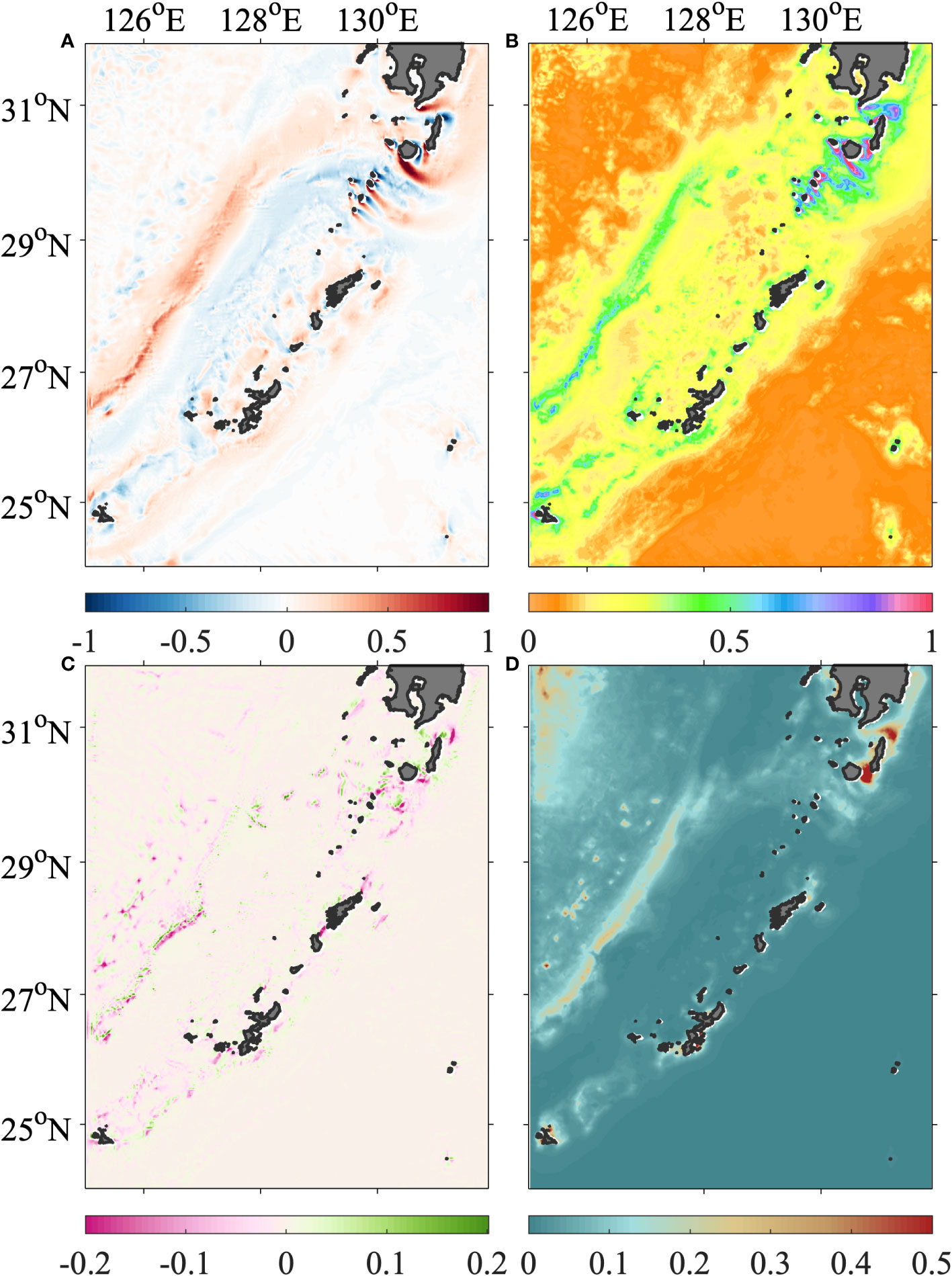
Figure 2 Spatial distributions of (A) Rossby number (Ro=ζ/f), (B) normalized strain rate (ε/f), (C) normalized divergence (δ/f), and (D) normalized inverse Richardson number. All the results were vertically and temporally averaged from 2003 to 2012.
The high values of divergence (Figure 2C) and inverse Richardson number (Figure 2D) showed similar streaks on the continental slope, while the former also existed in the lee area of the Tokara Islands. The divergence is closely associated with the submesoscale motions (Rocha et al., 2016b). In frontal areas, it indicates a secondary circulation comprising of up- and downwelling forced by deformations of the flow (McWilliams, 2016). It is found from the plane distribution that the relative vorticity on the continental slope is positively skewed (Figure 2A). The inverse Richardson number represents the ratio of vertical shear to buoyancy. A high value indicates that the flow was also vertically sheared, which indicates sufficient kinetic energy to break the potential balance. High-wavenumber internal waves can provide such vertical shear (Rainville and Pinkel, 2004). A high inverse Richardson number was also suggested to broaden the symmetric instability regime and cause positive skewness of the relative vorticity (Buckingham et al., 2016).
The skewness of relative vorticity (hereafter, skewness) is also a typical footprint of the submesoscale dynamics (Buckingham et al., 2016; Rocha et al., 2016a) and often arises along with a high Rossby number. This indicates asymmetry or an imbalance between positive and negative relative vorticity, which is commonly exhibited in small structures (e.g., filaments). Statistical results are presented in the probability distribution density domain of vorticity vs. strain rate (Figure 3). On the continental slope, the basic distribution (Figure 3A) showed apparent leaning to one side; the overall skewness was 0.83. For layers 0–200 m, 200–400 m, and deeper than 400 m (Figures 3B–D), the values were 0.67, 1.20, and 0.26, respectively. The maximum value at the intermediate depths indicates that it may be associated with mixed-layer instability. For the entire lee area (Figures 3E–H), the distribution was stretched to both sides, and the corresponding skewness was 0.20, 0.28, −0.10, and 0.21, respectively. Although the values were much weaker than those on the continental slope, it should be noted that the skewness is actually bi-directional. Each channel between islands, capes, and seamounts was either strongly positively or negatively skewed (Figure 2A). Thus, regional results counteracted alternately spread refined structures with reverse-sign vorticities.
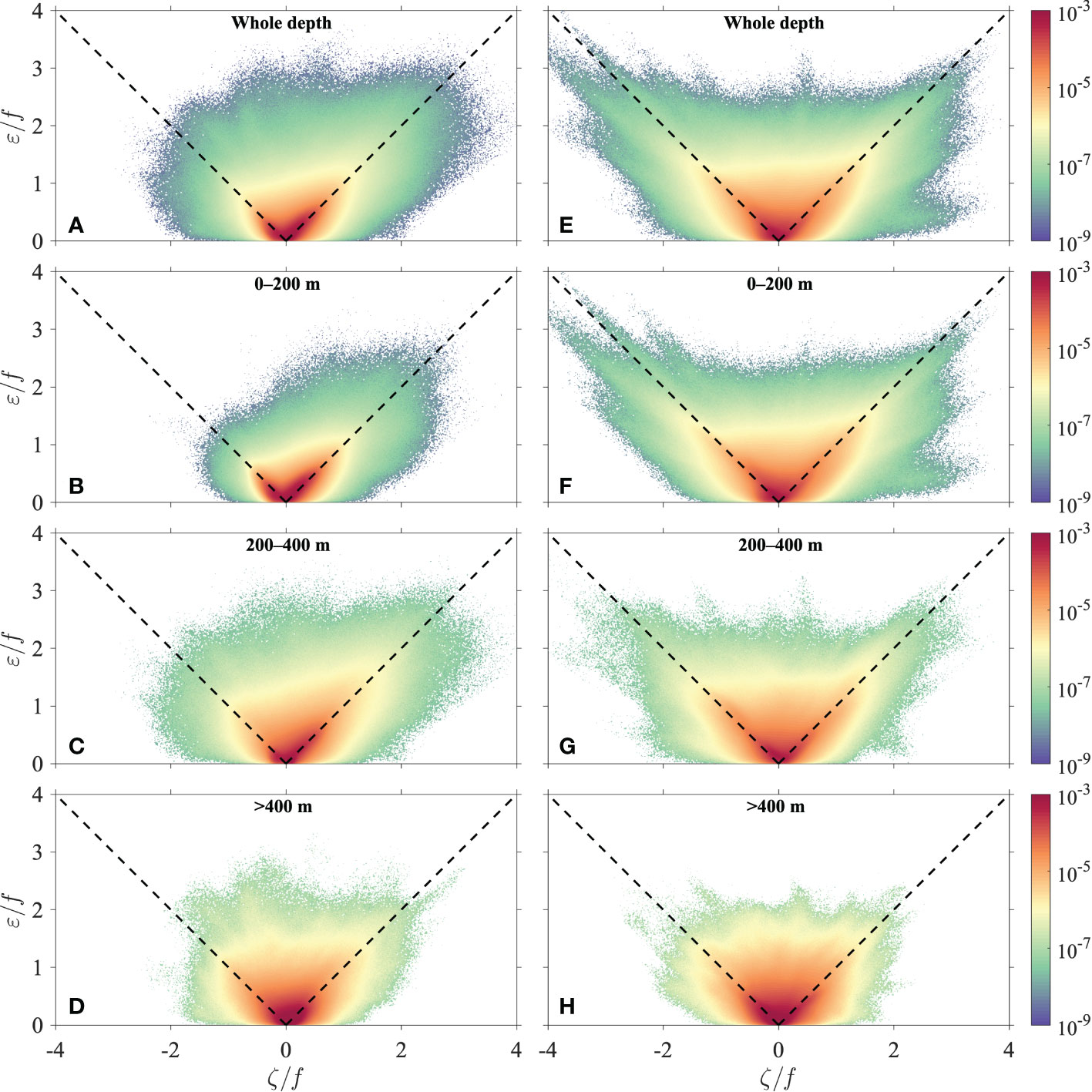
Figure 3 Statistics for the joint probability density distribution of strain rate vs. relative vorticity of different layers from 2003 to 2012. The domain was classified using a bin size of 0.01, and the values were normalized by the sum of each layer. Two diagonal dashed lines corresponded to ε=±ζ. The left (A–D) and right (E, F) panels correspond to the continental slope area for the Kuroshio before turning directly to the strait and lee area of the Tokara Strait for the Kuroshio after flowing through the Tokara Islands, respectively.
The Rossby number exceeded ±3 for extreme values, meanwhile, showing alignment with the reference lines of ε=±ζ (Figure 3). This indicated that the fluid was not purely rotational like a rigid body but was deformed simultaneously when rotating, which implied shear flow motions in the submesoscale fronts (Shcherbina et al., 2013). On the continental slope (Figures 3A–D), cyclonic motions reflected such natures intensely, but anticyclonic motions did not, similar to mesoscale eddies or advection motions. While it is distinct in the lee area (Figures 3E–H), both cyclonic and anticyclonic motions were strongly connected with the strain rate and could reach larger extreme values. This was also consistent with the spectral analysis results (Figures 1F, G).
The spatial distributions of skewness and standard deviation (Figure 4) further suggested that salient topographic features were largely responsible for the generation of submesoscale features. Before flowing through the Tokara Islands, high skewness and standard deviation values in the Kuroshio formed a long strip along the slope. The Tokara Islands functioned as sieves, filtering out multiple smaller structures corresponding to mesh sizes and improved their ratios to be more dynamically active, as well as enhancing biochemistry processes through turbulent mixing (Hasegawa et al., 2021). This may be because the narrowing of the water passages decreased the potential and increased kinetic energy (Bernoulli’s principle for incompressible fluid), which was injected into the submesoscale regimes. Strong variability arose, except in the aforementioned continental slope, the lee area of the TkS, and the vicinity around the Ryukyu Islands, even around a very small and inconspicuous island at ~131.2°E in the Pacific, which merits future investigation and is not discussed here.
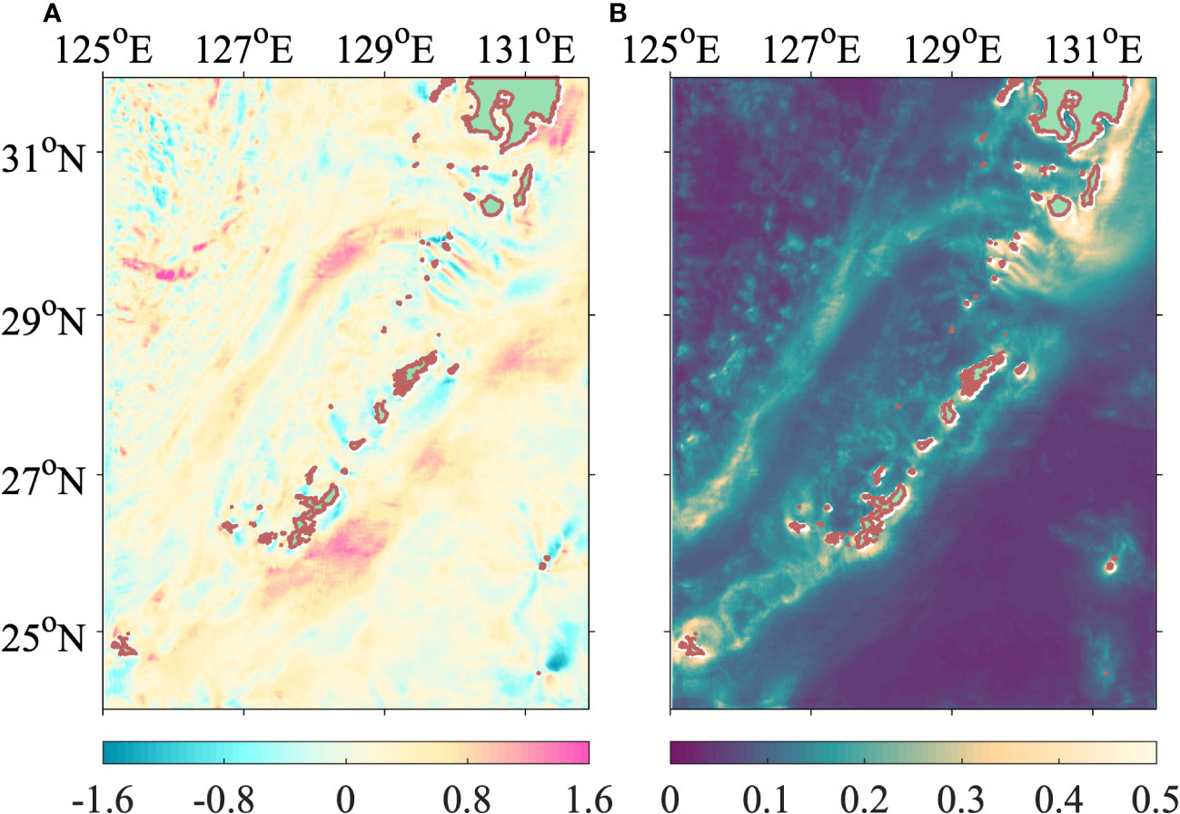
Figure 4 Depth-averaged (A) skewness and (B) standard deviation of Rossby number during 2003–2012.
4. Variabilities
Although the long-term temporal average may have dampened or smoothened some extremely high values associated with transient processes, the submesoscale characteristics were prominent and manifested in the climatological results (Section 3) for the Kuroshio region. This may be because the contribution factors, the topographic features, and the Kuroshio, were long-lasting and served as an incessant energy source. Based on the mean state, variabilities of the Kuroshio were exhibited due to intrinsic or extrinsic factors (Nakamura et al., 2008; Nakamura et al., 2016) and were naturally supposed to induce corresponding variations in submesoscale dynamics if they were coupled. In addition to the dynamical driving forces, background conditions (such as stratification) can also contribute to the generation of submesoscale (Zhang et al., 2020). In this section, the relevant variabilities are investigated.
4.1. Seasonality
The spatial pattern (Figure 2) indicates that steep topography contributed to a high Rossby number, which was highly related to the strong strain rate (Figure 3), implying submesoscale characteristics. Quantitatively, the correlation coefficients between Rossby number and strain rate throughout the whole period had average values of 0.58 in the continental slope and 0.57 in the lee area of the TkS, suggesting a long-lasting mechanism in which the submesoscale largely originated from the topographic strain rate. Moreover, the former (Figure 5A) exhibited clear dominant interannual or seasonal signals with valley and peak values in summer and winter, respectively, and was positively correlated with the seasonal variations in mixed-layer depth but with marginal phase lags (Figure 5A). That is, when the mixed layer became deeper in winter, the submesoscale was easier to be produced by the strain. In summer, stronger solar heat radiation results in a larger temperature gradient, stronger stratification, and shallower mixed-layer depth, reflecting higher mixed-layer stability and more stored gravitational potential energy. Conversely, the vertical water column became weakly stratified in winter, deepening the mixed layer, enabling instabilities to develop more fully, and releasing more kinetic energy. This modulation depended on atmospheric forcing and was reported to elevate mesoscale and submesoscale kinetic energy levels twofold in the North Pacific (Sasaki et al., 2014).
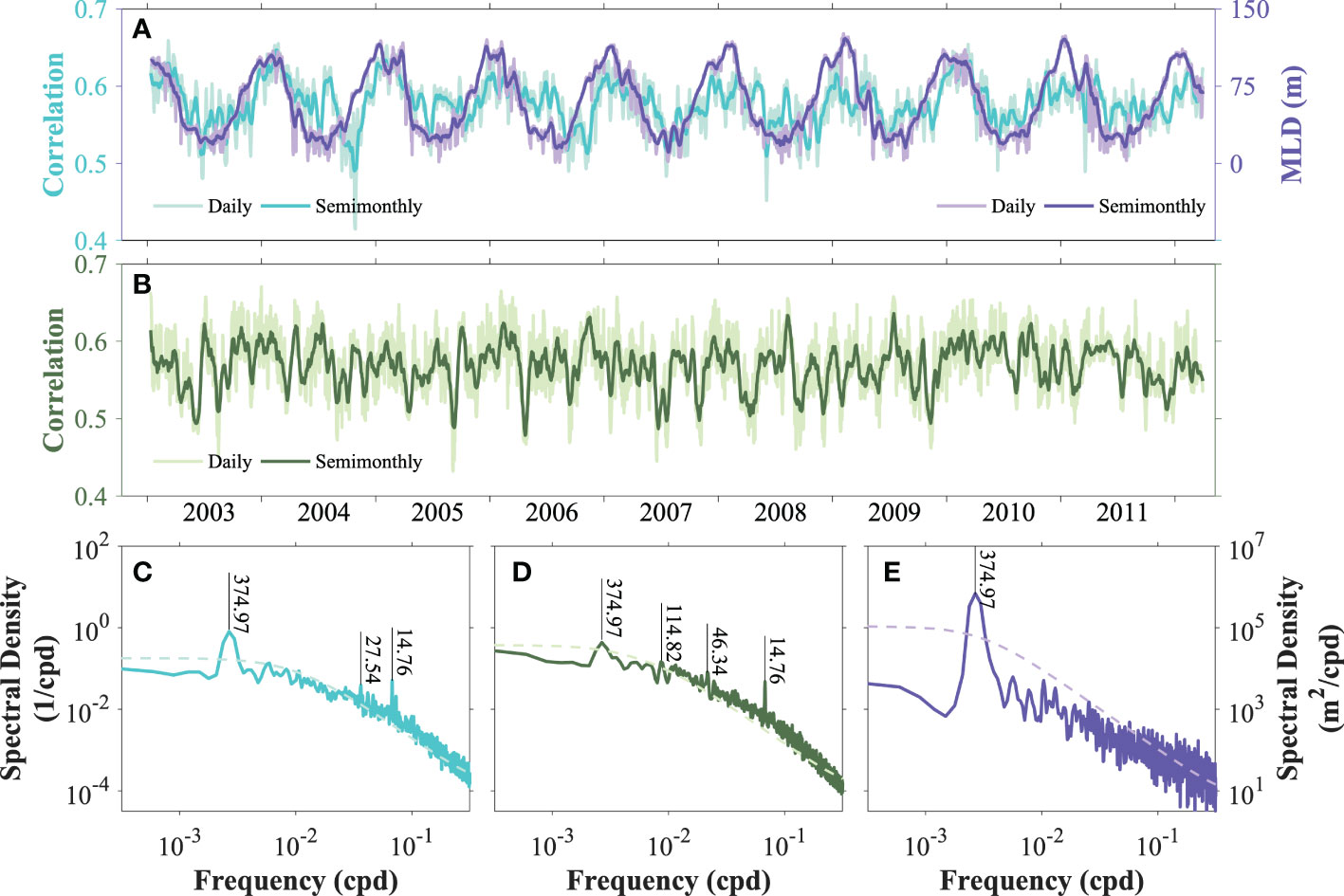
Figure 5 (A) Time series of the spatial correlation coefficient between Rossby number and strain rate (cyan lines) on the continental slope, and (B) those in the lee area of the Tokara Strait. Time series of mixed-layer depth (purple lines) in the continental slope, defined as the depth with the strongest stratification, were superimposed in (A). The thin lines in lighter colors indicated daily results, while the thick lines in deeper colors were semimonthly smoothed. Frequency spectra of (C) spatial correlation time series in (A), (D) mixed-layer depth time series in (A), and (E) spatial correlation time series in (B). The dashed lines represented a 95% significance level estimated by the red noise spectrum. Major spectral peaks were marked by corresponding periods above.
However, in the lee area of the TkS, the seasonal cycle of correlation could not be visually discerned (Figure 5B), although the mixed layer here was also seasonally modulated (not shown). This distinction signified the possibility that instabilities in the mixed layer were less important in affecting topographic strain-induced production in the submesoscale. This may be because the long-persisting flow–topography interactions, contributing to almost a two-order elevation of turbulent mixing (Tsutsumi et al., 2017; Nagai et al., 2021), were much stronger than other areas (e.g., Figure 2B) and more effective than other instabilities.
The period of this seasonality was ~374.97 days (Figure 5E), which was dominant on the continental slope (Figure 5C) and weaker in the lee area of the TkS (Figure 5D). In particular, spectral peaks with tidal periods of ~14.76 and ~27.54 days were noticeable, although tidal constituents were filtered out from the model data. This implies that the consequent effects associated with tidal processes were not ephemeral and were retained in the background conditions. The tides may have generated IGWs or internal-wave continuum, whose overlap in submesoscale ranges and corresponding influence were still exhibited after detiding. More detailed mechanisms should be investigated in the future. In addition, weak intraseasonal periods of ~46.34 and ~114.52 days in the TkS may be related to background current field variabilities, the Kuroshio meander, which included similar periods (Nakamura et al., 2006). Meander occurrence meant that the current velocity cores of the Kuroshio had shifted (Liu et al., 2019), causing intensity variation of flow–topography interaction, a pathway of submesoscale arising in the presence of massive topographic features (see Section 3).
Daily kinetic energy wavenumber spectra along the Kuroshio axis and the corresponding spectral slopes (Figure 6C), reflecting the governed power laws of fluid mechanics and potential energy cascades, were obtained to gain more insights into the variabilities of submesoscale dynamics. These values (Figure 6C) varied over a relatively wide range. A conspicuous and nonstationary separatrix at a depth of ~150 m divided the two regimes with distinct dynamics, showing a dynamic transition and depth dependence. The upper layers above ~150 m showed steeper slopes around −3, which implies dominant quasi-geostrophic dynamics (e.g., Wang et al., 2010; Rocha et al., 2016a). The steeper spectral slopes, which are approximately confined to this depth range at most times, fluctuated temporally with the amplitude increase/decrease and upward/downward penetration. A depth of 150 m was close to the lower limit of the mixed layer (Figure 5A). These suggest that the dynamics of the upper layers may also be influenced by mixed-layer instabilities. For layers below ~150 m, the slopes were flatter around −2 and had a relatively smaller variation. Slope variation implies that kinetic energy was redistributed across scales, changing the submesoscale energy content. Correspondingly, the spectra for the two regimes were equal at scales between 100 and 1,000 km but presented observable differences at submesoscale ranges smaller than 100 km (Figure 6A). The submesoscale energy level of the lower layers elevated, and the spectra became flattened.
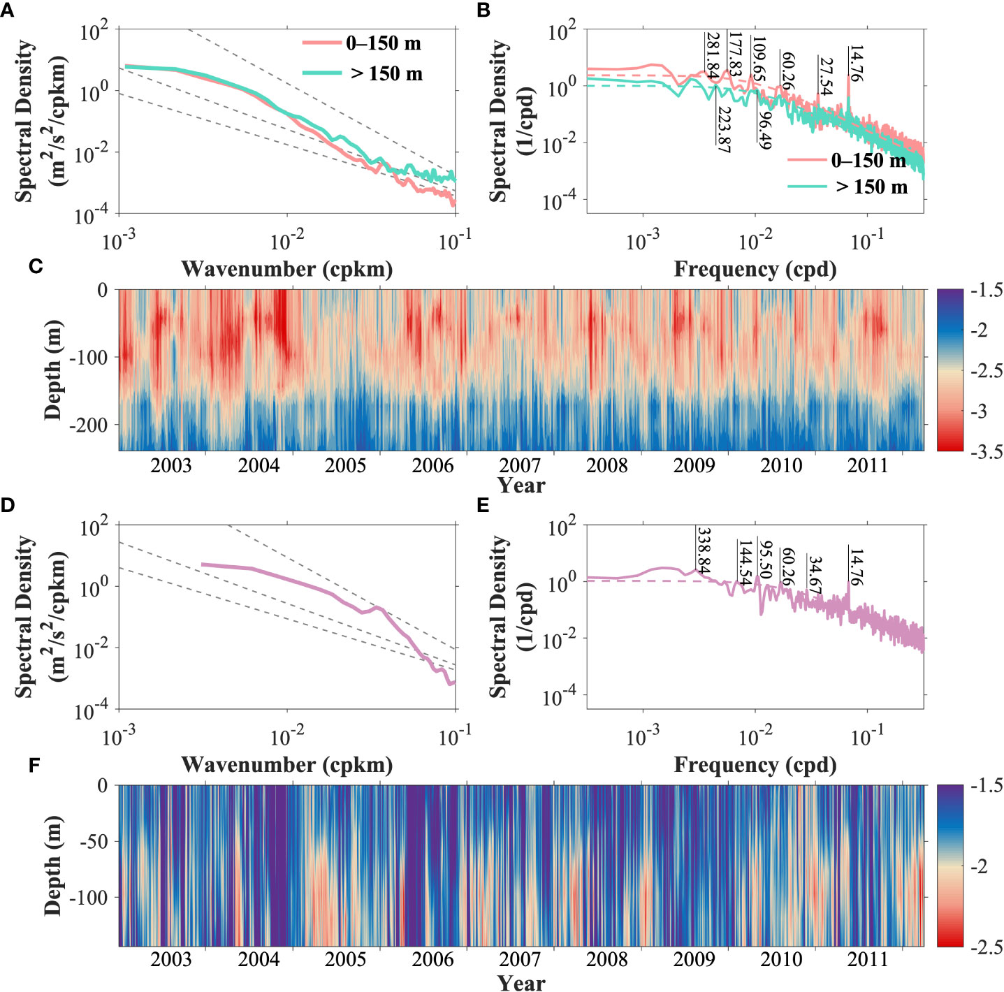
Figure 6 (A) Kinetic energy wavenumber spectra along the Kuroshio axis, averaged between 2003 and 2012. Spectra of layers above (pink) and below (green) 150 m were separately vertically averaged. Power laws of k−5/3, k−2, and k−3 were presented by gray dashed lines. (B) Frequency spectra of linearly fitted slopes of wavenumber spectra for scales larger than 20 km (~10−1.3 cpkm). They were calculated for each layer and separately averaged above (pink) and below (green) 150 m. Colored dashed lines were at the 95% significance level estimated by the red noise spectrum. (C) Time series of linearly fitted slopes of wavenumber spectra. Some typical spectral peaks were marked by corresponding periods. (D–F) Same as (A–C), respectively, but for sections across the Kuroshio in the Tokara Strait (Figure 1C) and were not averaged separately for the upper and lower layers. The (F) had a shallower depth range than the (C) because the data sampling was not continuous after being influenced by underwater seamounts in the strait.
Temporally, periods of the slopes were more diversified (Figure 6B) than those of the spatial correlation between Rossby number and strain rate (Figures 5C, E). Variation in the slopes indicated redistribution of kinetic energy across scales and can be classified as and traced back to the effects of the tide (14.76 and 27.54 days), the Kuroshio path meander (30–220 days), and seasonality (>300 days). The last two were incompletely equivalent to the previous estimates (Figures 5C, E), possibly because the detailed processes were more complex and not only strain-induced. The spectral amplitudes of the upper layers were (Figure 6B) stronger than those of the lower layers, consistent with larger variations in the slopes.
The averaged kinetic energy spectra across the Kuroshio in the TkS (Figure 6D) became flattened, almost obeying the −5/3 law (Callies and Ferrari, 2013), and showed energy injection at the submesoscale, which was probably topography-induced (as discussed in Section 3.2). The flatter spectral slopes (Figure 6F), which present a smaller amplitude range, were also not stabilized. The corresponding temporal variabilities (Figure 6E) were plentiful and fell into the abovementioned three categorized contribution factors, among which tidal variabilities were fixed while the Kuroshio meander and seasonality had regional differences.
In general, it was found that the governing dynamics of kinetic energy, which vary temporally and spatially, should not be interpreted solely by a single turbulence theory. The combined works of multiple processes can result in remarkable changes in the dynamical regime, most of which may be submesoscale.
4.2. Kuroshio oscillation effect
As discussed, some intra-annual signals of multi-scale kinetic energy dynamics are probably related to the modulation of variabilities of the Kuroshio. The analytical results of the frequency spectrum had well-extracted footprints of the Kuroshio (Figure 7B). The strongest spectral energy is just along the Kuroshio path, indicating a large derivation from the Kuroshio variabilities, which are dynamically dominant. Notably, the energy path in the ECS was approximately divided into two streaks, distributed on both sides of the climatological mean Kuroshio axis. This feature was previously less focused and surmised to be the result of the Kuroshio path meander, which occurs when the Kuroshio axis oscillated and shifts bilaterally. An energetic area at ~26°N, ~125.5°E may be related to frequent eddy activity arising from the Pacific (Andres et al., 2008) when lacking blockage of the Ryukyu Islands. The periods (Figure 7A) of the Kuroshio variability in the ECS showed regional differences but were basically consistent with the above estimations.
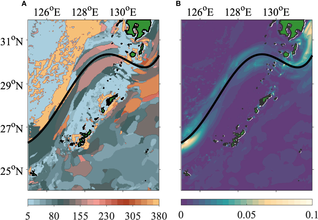
Figure 7 (A) Periods (unit: day) of the strongest frequency spectral amplitudes above the 95% significance level. (B) The corresponding strongest frequency spectral amplitudes (unit: m2/s2) above the 95% significance level. The spectra were calculated for the current velocity field during 2003–2012 and vertically averaged. Black thick lines represented the mean Kuroshio axis during 2003–2012.
The occurrence of the Kuroshio path meander can be further traced back to the dimensional growth of eddies downstream along the continental slope, generated in fronts due to baroclinic instabilities (Nakamura, 2005). Eddies with increasing spatial sizes would become an obstruction and force the Kuroshio to deviate from the original path. Following this, the eddies generated on both sides of the Kuroshio axis and the corresponding evolution features could be used as metrics to evaluate the oscillation of the Kuroshio. Eddy statistics were detected on both sides of the Kuroshio mean axis along the Kuroshio flow direction. In the process of downstream propagation, the eddy group on the right side of the Kuroshio axis exhibited a dying trend with a gradual reduction in radii and was mainly located south of 29°N (Figure 8B). Conversely, the eddy group on the left side of the Kuroshio grew and reached maturity between 30°N and 32°N (Figure 8A), which is also the most active region of the Kuroshio path meander in the west of the TkS (Nakamura, 2005). This was consistent with previous knowledge that eddies attained full sizes in the west of the TkS and forced a transition of the Kuroshio in the TkS from a north path state to a south path state, which then triggered the path meander (Nakamura et al., 2003; Nakamura, 2005). These indicate that the left-side eddies represented the variability of the Kuroshio path meander. Temporally, the left-side eddy group had similar periods (Figure 8C) to those of the power laws, which are supposed to be caused by the Kuroshio path meander (Figures 6B, E), while the right-side eddy group exhibited a seasonal signal (Figure 8D). Therefore, more evidence suggests that large-scale circulation oscillation triggered by eddy activities would affect the submesoscale dynamics.
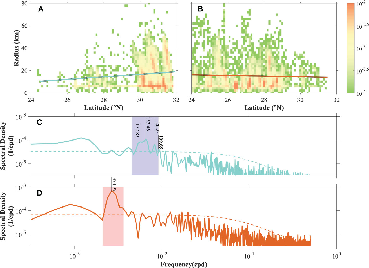
Figure 8 The probability density distribution of horizontal radii for eddies is classified into two groups: one on the (A) left and another on the (B) right sides of the mean Kuroshio axis along the flow direction. The cyan and orange lines were linearly fitted trends of eddy radiuses for latitudes. Only those eddies with northeastward propagation were retained. The others were removed. Frequency spectra for existing numbers of eddies on the (C) left and (D) right sides of the mean Kuroshio axis along the flow direction. Dashed lines were 95% significance levels estimated by the red noise spectra. Typical spectral period ranges were marked using purple and pink shading, which represented ~109–224 days (i.e., ~10−2.35–10−2.04 cpd) in (C) and ~275–478 days (i.e., ~10−2.68–10−2.44 cpd) in (D), respectively.
5. Conclusions
High-resolution numerical simulations revealed that the large-scale western boundary current in the ECS, the Kuroshio, was also a reservoir of remarkably elevated submesoscale energy. The submesoscale footprints arose with extraordinarily high Rossby numbers in a line or streak pattern, mainly along the continental slope and downstream of the islands in the TkS, which were both salient in steep topographical features. The topographic-induced strain rate contributed significantly to the production of the submesoscale. This resulted in a positively skewed distribution of the Rossby number on the continental slope but a strongly bidirectional skewness in the lee area of the TkS. Amid the effects of multiple processes, including internal tides, mixed-layer instabilities, and the Kuroshio path meander, temporal variabilities in submesoscale dynamics arose. The last one was evaluated using eddy activities, which further pointed out a closely connected system among different dynamical processes across scales. These results provided a basic pattern and discussed hotspots of submesoscale and corresponding multi-scale interactions in the ECS, which have implications for future studies and field observation setups.
The real conditions are more complex; therefore, open questions remain to be addressed, such as the evaluation of wind in the ECS in generating submesoscale turbulence. Moreover, it appears to be a complete chain in which eddies can trigger the Kuroshio path meander, which then induces variabilities at the submesoscale. However, the fluctuating Kuroshio changed the background conditions related to baroclinic instabilities, which are grounds for eddy generation. In addition, submesoscale processes affect the intensity of fronts, which may also affect the frontal eddy in turn. The detailed mechanisms and precise contribution ratios remain unknown.
Data availability statement
The original contributions presented in the study are included in the article/Supplementary Material. Further inquiries can be directed to the corresponding author.
Author contributions
JC contributed to the conception and design of the study. X-HZ provided the model and observational datasets. All authors contributed to the article and approved the submitted version.
Funding
This study was supported by the National Natural Science Foundation of China (Grant No. 41920104006); Scientific Research Fund of Second Institute of Oceanography, MNR (Grant No. JZ2001 and QNYC2102); Project of State Key Laboratory of Satellite Ocean Environment Dynamics, Second Institute of Oceanography (SOEDZZ2106, SOEDZZ2207); Innovation Group Project of Southern Marine Science and Engineering Guangdong Laboratory (Zhuhai) (No. 311020004); and the Oceanic Interdisciplinary Program of Shanghai Jiao Tong University (project number SL2021MS021).
Conflict of interest
The authors declare that the research was conducted in the absence of any commercial or financial relationships that could be construed as a potential conflict of interest.
Publisher’s note
All claims expressed in this article are solely those of the authors and do not necessarily represent those of their affiliated organizations, or those of the publisher, the editors and the reviewers. Any product that may be evaluated in this article, or claim that may be made by its manufacturer, is not guaranteed or endorsed by the publisher.
References
Alford M. H., MacKinnon J. A., Simmons H. L., Nash J. D. (2016). Near-inertial internal gravity waves in the ocean. Annu. Rev. Mar. Sci. 8, 95–123. doi: 10.1146/annurev-marine-010814-015746
Alford M. H., Peacock T., MacKinnon J. A., Nash J. D., Buijsman M. C., Centurioni L. R., et al. (2015). The formation and fate of internal waves in the south China Sea. Nature 521, 65–69. doi: 10.1038/nature14399
Andres M., Cenedese C. (2013). Laboratory experiments and observations of cyclonic and anticyclonic eddies impinging on an island: EDDIES IMPINGING ON AN ISLAND. J. Geophys. Res. Oceans 118, 762–773. doi: 10.1002/jgrc.20081
Andres M., Park J.-H., Wimbush M., Zhu X.-H., Chang K.-I., Ichikawa H. (2008). Study of the Kuroshio/Ryukyu current system based on satellite-altimeter and in situ measurements. J. Oceanogr. 64, 937–950. doi: 10.1007/s10872-008-0077-2
Buckingham C. E., Naveira Garabato A. C., Thompson A. F., Brannigan L., Lazar A., Marshall D. P., et al. (2016). Seasonality of submesoscale flows in the ocean surface boundary layer. Geophys. Res. Lett. 43, 2118–2126. doi: 10.1002/2016GL068009
Callies J., Ferrari R. (2013). Interpreting energy and tracer spectra of upper-ocean turbulence in the submesoscale range (1–200 km). J. Phys. Oceanogr. 43, 2456–2474. doi: 10.1175/JPO-D-13-063.1
Davidson P. A. (2015). Turbulence: an introduction for scientists and engineers (Second edition. Oxford, United Kingdom; New York, NY, United States of America: Oxford University Press).
Gula J., Molemaker M. J., McWilliams J. C. (2015). Topographic vorticity generation, submesoscale instability and vortex street formation in the gulf stream. Geophys. Res. Lett. 42, 4054–4062. doi: 10.1002/2015GL063731
Gula J., Molemaker M. J., McWilliams J. C. (2016). Topographic generation of submesoscale centrifugal instability and energy dissipation. Nat. Commun. 7, 12811. doi: 10.1038/ncomms12811
Hasegawa D., Matsuno T., Tsutsumi E., Senjyu T., Endoh T., Tanaka T., et al. (2021). How a small reef in the kuroshio cultivates the ocean. Geophys. Res. Lett. 48, e2020GL092063. doi: 10.1029/2020GL092063
Klein P., Lapeyre G. (2009). The oceanic vertical pump induced by mesoscale and submesoscale turbulence. Annu. Rev. Mar. Sci. 1, 351–375. doi: 10.1146/annurev.marine.010908.163704
Liu Z., Nakamura H., Zhu X., Nishina A., Guo X., Dong M. (2019). Tempo-spatial variations of the kuroshio current in the tokara strait based on long-term ferryboat ADCP data. J. Geophys. Res. Oceans 124, 6030–6049. doi: 10.1029/2018JC014771
McWilliams J. C. (2016). Submesoscale currents in the ocean. Proc. R. Soc A. 472, 20160117. doi: 10.1098/rspa.2016.0117
Nagai T., Hasegawa D., Tsutsumi E., Nakamura H., Nishina A., Senjyu T., et al. (2021). The kuroshio flowing over seamounts and associated submesoscale flows drive 100-km-wide 100-1000-fold enhancement of turbulence. Commun. Earth. Environ. 2, 170. doi: 10.1038/s43247-021-00230-7
Nakamura H. (2005). Numerical study on the kuroshio path states in the northern Okinawa trough of the East China Sea. J. Geophys. Res. Oceans 110, C04003. doi: 10.1029/2004JC002656
Nakamura H., Hiranaka R., Ambe D., Saito T. (2016). “Local wind effect on the kuroshio path state off the southeastern coast of kyushu,” in “Hot spots” in the climate system (Tokyo: Springer), 109–130. doi: 10.1007/978-4-431-56053-1_7
Nakamura H., Ichikawa H., Nishina A., Lie H. (2003). Kuroshio path meander between the continental slope and the tokara strait in the East China Sea. J. Geophys. Res. Oceans, 108(C11). doi: 10.1029/2002JC001450
Nakamura H., Nishina A., Ichikawa H., Nonaka M., Sasaki H. (2008). Deep countercurrent beneath the kuroshio in the Okinawa trough. J. Geophys. Res. Oceans 113, C06030. doi: 10.1029/2007JC004574
Nakamura H., Yamashiro T., Nishina A., Ichikawa H. (2006). Time-frequency variability of kuroshio meanders in tokara strait. Geophys. Res. Lett. 33, L21605 doi: 10.1029/2006GL027516
Nencioli F., Dong C., Dickey T., Washburn L., Mcwilliams J. C. (2010). A vector geometry–based eddy detection algorithm and its application to a high-resolution numerical model product and high-frequency radar surface velocities in the southern California bight. J. Atoms. Oceanic. Technol. 27, 16. doi: 10.1175/2009JTECHO725.1
Pezzi L. P., de Souza R. B., Santini M. F., Miller A. J., Carvalho J. T., Parise C. K., et al. (2021). Oceanic eddy-induced modifications to air–sea heat and CO2 fluxes in the Brazil-malvinas confluence. Sci. Rep. 11, 10648. doi: 10.1038/s41598-021-89985-9
Qiu B., Nakano T., Chen S., Klein P. (2017). Submesoscale transition from geostrophic flows to internal waves in the northwestern pacific upper ocean. Nat. Commun. 8, 14055. doi: 10.1038/ncomms14055
Qiu B., Nakano T., Chen S., Klein P. (2022). Bi-directional energy cascades in the pacific ocean from equator to subarctic gyre. Geophys. Res. Lett. 49, e2022GL097713. doi: 10.1029/2022GL097713
Rainville L., Pinkel R. (2004). Observations of energetic high-wavenumber internal waves in the kuroshio. J. Phys. Oceanogr. 34, 1495–1505. doi: 10.1175/1520-0485(2004)034<1495:OOEHIW>2.0.CO;2
Rocha C. B., Chereskin T. K., Gille S. T., Menemenlis D. (2016a). Mesoscale to submesoscale wavenumber spectra in drake passage. J. Phys. Oceanogr. 46, 601–620. doi: 10.1175/JPO-D-15-0087.1
Rocha C. B., Gille S. T., Chereskin T. K., Menemenlis D. (2016b). Seasonality of submesoscale dynamics in the kuroshio extension. Geophys. Res. Lett. doi: 10.1002/2016GL071349
Rosso I., Hogg A., Mc C., Kiss A. E., Gayen B. (2015). Topographic influence on submesoscale dynamics in the southern ocean. Geophys. Res. Lett. 42, 1139–1147. doi: 10.1002/2014GL062720
Ruan X., Thompson A. F., Flexas M. M., Sprintall J. (2017). Contribution of topographically generated submesoscale turbulence to southern ocean overturning. Nat. Geosci. 10, 840–845. doi: 10.1038/ngeo3053
Sasaki H., Klein P., Qiu B., Sasai Y. (2014). Impact of oceanic-scale interactions on the seasonal modulation of ocean dynamics by the atmosphere. Nat. Commun. 5, 5636. doi: 10.1038/ncomms6636
Shcherbina A. Y., D’Asaro E. A., Lee C. M., Klymak J. M., Molemaker M. J., McWilliams J. C. (2013). Statistics of vertical vorticity, divergence, and strain in a developed submesoscale turbulence field: SUBMESOSCALE TURBULENCE STATISTICS. Geophys. Res. Lett. 40, 4706–4711. doi: 10.1002/grl.50919
Tsutsumi E., Matsuno T., Lien R., Nakamura H., Senjyu T., Guo X. (2017). Turbulent mixing within the kuroshio in the tokara strait. J. Geophys. Res. Oceans 122, 7082–7094. doi: 10.1002/2017JC013049
Varlamov S. M., Guo X., Miyama T., Ichikawa K., Waseda T., Miyazawa Y. (2015). M2 baroclinic tide variability modulated by the ocean circulation south of Japan. J. Geophys. Res. Oceans 120, 3681–3710. doi: 10.1002/2015JC010739
Wang D.-P., Flagg C. N., Donohue K., Rossby H. T. (2010). Wavenumber spectrum in the gulf stream from shipboard ADCP observations and comparison with altimetry measurements. J. Phys. Oceanogr. 40, 840–844. doi: 10.1175/2009JPO4330.1
Xie J.-H. (2020). Downscale transfer of quasigeostrophic energy catalyzed by near-inertial waves. J. Fluid Mech. 904, A40. doi: 10.1017/jfm.2020.709
Yan X., Kang D., Curchitser E. N., Pang C. (2019). Energetics of eddy–mean flow interactions along the Western boundary currents in the north pacific. J. Phys. Oceanogr. 49, 789–810. doi: 10.1175/JPO-D-18-0201.1
Zhang Z., Qiu B. (2020). Surface chlorophyll enhancement in mesoscale eddies by submesoscale spiral bands. Geophys. Res. Lett. 47, e2020GL088820. doi: 10.1029/2020GL088820
Keywords: eddy-current interaction, Kuroshio, submesoscale, topography, East China Sea
Citation: Chen J, Zhu X-H, Zheng H and Wang M (2023) Submesoscale dynamics accompanying the Kuroshio in the East China Sea. Front. Mar. Sci. 9:1124457. doi: 10.3389/fmars.2022.1124457
Received: 15 December 2022; Accepted: 31 December 2022;
Published: 19 January 2023.
Edited by:
Fangguo Zhai, Ocean University of China, ChinaCopyright © 2023 Chen, Zhu, Zheng and Wang. This is an open-access article distributed under the terms of the Creative Commons Attribution License (CC BY). The use, distribution or reproduction in other forums is permitted, provided the original author(s) and the copyright owner(s) are credited and that the original publication in this journal is cited, in accordance with accepted academic practice. No use, distribution or reproduction is permitted which does not comply with these terms.
*Correspondence: Xiao-Hua Zhu, eGh6aHVAc2lvLm9yZy5jbg==