Tomographic reconstruction of 3D sound speed fields to reveal internal tides on the continental slope of the South China Sea

Mirror-type coastal acoustic tomography (MCAT) is an advancement of coastal acoustic tomography (CAT) with a mirror function that enables the nearshore transmission of offshore observation data. Subsurface MCATs are used to monitor small-scale oceanographic phenomena over large areas on the continental slope of the South China Sea (300–1,000 m). This study investigated the performance of MCAT network observation for internal tide monitoring using 3D tomographic inversion. MCAT facilitates communication with each other and is networked. Results of 3D tomographic inversion were highly consistent with the Stanford unstructured nonhydrostatic terrain-following adaptive Navier–Stokes (SUNTANS) model data. The root-mean-square difference of the sound speed obtained by the inversion method was< 1.0 m/s. The high sound speeds induced by the internal tide were well captured by the results of 3D inversion. A high sound speed band of > 1,516 m/s was used as an index of internal tides, which propagated at a speed of 1.9 m/s. Sensitivity experiments demonstrated that a swing of the anchor tether of< 5 m had less impact on sound speed inversion, while distance drifts caused by human activities of > 50 m had a significant influence. The missing of one or several stations owing to natural factors did not generate significant variations in the results of network observation. This study demonstrated that the MCAT network observation strategy, equipped with numerous stations, is more effective in capturing the characteristics of internal tides.

1. Introduction

Acoustic waves are known to be the best signals for long-distance transmission in the ocean, and ocean dynamic processes such as internal waves, tidal currents, and mesoscale eddies are affected by them. Ocean acoustic tomography (OAT) is an effective tool for measuring mesoscale phenomena in oceans. OAT has a special advantage in obtaining the sound speed and current velocity fields from acoustic travel time measured in mesoscale ranges (Wunsch, 1979). In 1981, the Woods Hole Oceanographic Institution led the first ocean acoustic tomography experiment in the Bermuda Sea (area = 300 × 300 km) south of the Gulf Stream and successfully obtained the three-dimensional (3D) structure of mesoscale eddies, which proved the feasibility of the acoustic tomography method for ocean observation (The Ocean Tomography Group, 1982). Later, a series of OAT experiments was conducted in the United States, Japan, and Europe (Cornuelle et al., 1989; Worcester et al., 1993; Send et al., 1995; Yuan et al., 1999) and mesoscale ocean phenomena such as the Kuroshio meander and deep-sea convection were successfully observed. OAT is a novel approach to simultaneously observe the 3D sound speed fields of ocean mesoscale phenomena. However, owing to the constraints of human and material resources, it is difficult to organize a large number of OAT in the observation domain of several hundred kilometers for small- and medium-scale dynamic processes.

The coastal acoustic tomography (CAT) system was designed by the Hiroshima University based on the advanced technologies of OAT for the observation of small-scale ocean dynamic phenomena in coastal seas. Many CAT observations have been successfully achieved near the shore (Zheng et al., 1997; Zheng et al., 1998; Yamoaka et al., 2002; Yamaguchi et al., 2005; Zhu et al., 2013). Compared with OAT, CAT observations typically cover only tens or several tens of square kilometers; however, it has a higher observation frequency and finer spatiotemporal resolution to meet the requirements of coastal sea observations. CAT has demonstrated its ability to capture small-scale tidal vortices. Yamoaka et al. (2002) successfully captured the processes of initiation, growth, translation, and decay of tidal vortex pairs with five CAT stations in the Nekoseto Strait, Japan. Zhu et al. (2013) conducted a CAT experiment with seven stations in Zhitou Bay, Zhoushan, and observed the dynamic processes of small-scale tidal current circulation over a sea area of 12 × 12 km. On the other hand, Park and Kaneko (2001) and Zhu et al. (2017) assimilated CAT data into the ocean circulation model and reconstructed the fine flow field in the inland sea and around the island, respectively. Zhang et al. (2015) and Chen et al. (2017) discussed upwelling after typhoon passage by inversion and assimilation of CAT data obtained in Hiroshima Bay, Japan, respectively. The CAT is an innovative observation method for small-scale flow fields.

Mirror coastal acoustic tomography (MCAT) is an advanced form of CAT that is enhanced with a mirror module for travel time summation. MCAT is designed to transfer offshore observation data nearshore in real time using travel time summation. Chen et al. (2018) introduced the working principle of MCAT in detail and successfully conducted MCAT experiments in the Nekoseto Strait, Japan, thereby verifying its feasibility. Subsequently, Syamsudin et al. (2019) operated MCATs to successfully capture the subsurface structure of large waves, which were generated over a sill near the southern inlet of the Lombok Strait, Indonesia and propagated northward, demonstrating the superiority of MCAT. However, to date, the network observation of MCATs has never been realized for propagating internal waves.

The unique dual-ridge topography of the Luzon Strait in the South China Sea (SCS) interacts with barotropic tides to generate energetic internal tides and waves. Internal tides and waves generated in the Luzon Strait spread to > 1,600 km southwestward along the deep-sea basin of the SCS and reach the area around the Xisha Islands (Buijsman et al., 2010; Zhao, 2015). Some of them propagate to the western continental shelf of the SCS at shallower water depths. The internal tides amplified and their crests were steepened to generate internal solitary waves (Li and Farmer, 2011). The internal solitary waves continued to propagate westward and eventually disappear nearshore owing to bottom friction. The vicinity of islands and reefs in the SCS is also a place where internal waves and other small- and medium-scale dynamic phenomena are relatively active. In CAT, travel time data are generally stored in individual subsurface stations, and data analyses are performed after system recovery. It is relatively easy to recover the systems during normal estuarine observation; however, it is difficult to observe ocean phenomena in the SCS. The moored MCAT in real time is suitable for SCS for effectively monitoring the small- and medium-scale dynamic processed in the latter.

This study is based on the virtual MCAT network observation with the aim of simulating the 3D sound speed fields of mesoscale and sub-mesoscale dynamic phenomena (e.g., internal tides and waves) in the SCS. The possibility of observing internal wave propagation using an MCAT network based on results of simulation is discussed, and a theoretical basis is provided for future MCAT network observation.

2. Forward problem

2.1. Numerical model for internal tides

Hourly oceanographic conditions, with temperatures, salinities, and currents in the SCS, are modeled using the parallel, unstructured grid, non-hydrostatic ocean model termed Stanford unstructured nonhydrostatic terrain-following adaptive Navier–Stokes simulator (SUNTANS) (Fringer et al., 2006), with a mean resolution of 1,190 m, in the Luzon Strait, high-resolution grids with a minimum resolution of 89 m that were settled. The detailed description of the model configuration and performance analysis were presented in Zhang et al. (2011). A total of 336 h of data were obtained (21:00 January 3–21:00 January 17, 2018).

Figure 1A shows the amplitude of the isotherm induced by internal tides, which was estimated from the amplitude of the 15°C isotherm (Zhao et al., 2010; Zhang et al., 2011). The internal tides generated in the Luzon Strait (the amplitude of the 15°C isotherm was > 70 m) eventually propagate into the SCS. In this study, an experimental site (encircled with a black rectangle in Figure 1) was selected near the western edge of the high-amplitude area (~50 m) and adjacent areas of the Dongsha Islands. The high variations in temperature and salinity fields were attributed to the temporal variability of internal tides. Figure 1B shows an example of the sound speed field at hour 243, demonstrating that the experimental area was located in the area with a depth range of 300–1,000 m and featured energetic internal tides with a wavelength of ~82.1 km and phase speed of 1.9 m/s.

FIGURE 1

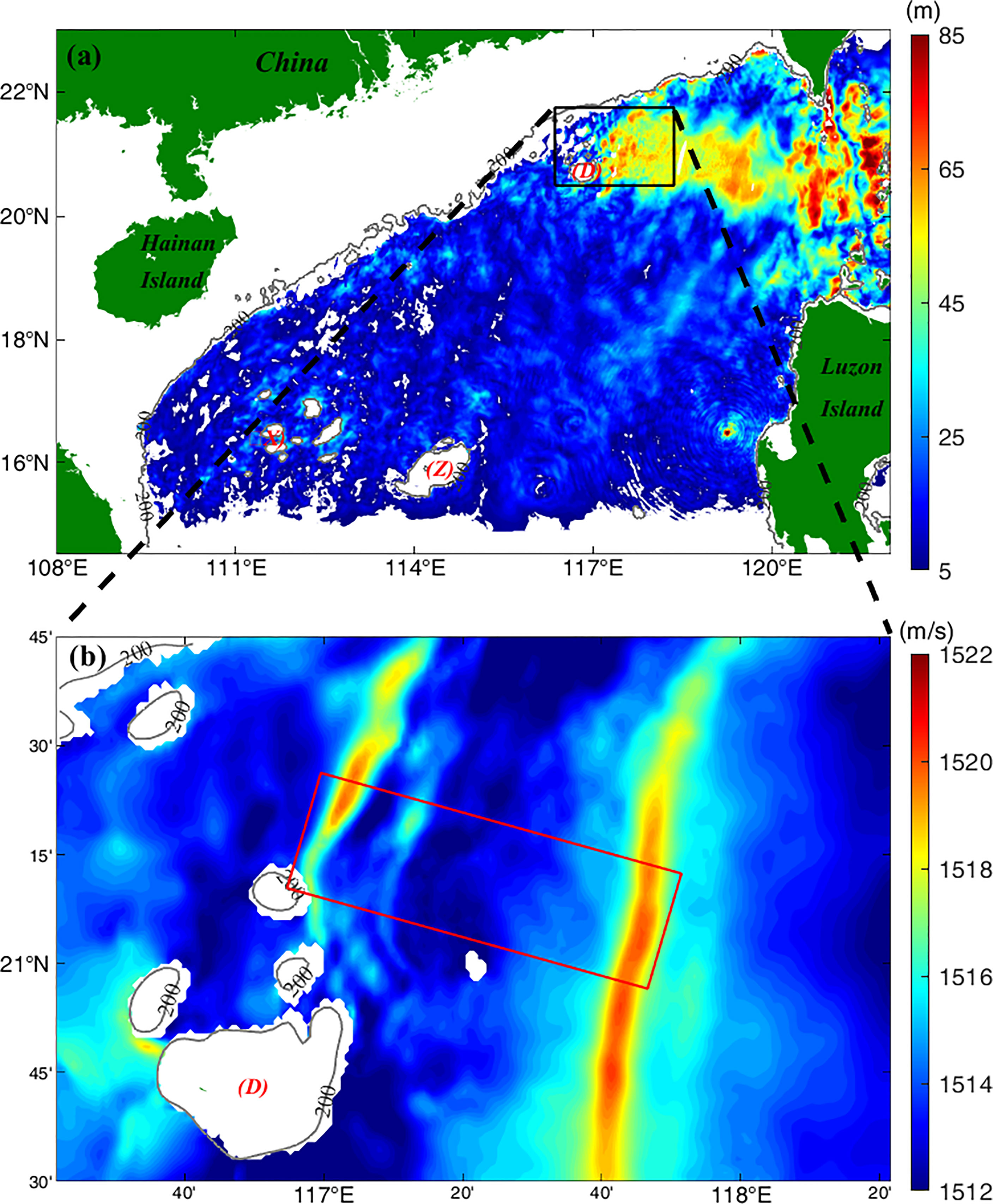
Figure 1 (A) Amplitude map of internal tides generated at hour 243 in the South China Sea during the application period of the SUNTANS model; (B) Magnified map of the area denoted by the black rectangle in (A) with color maps of sound speed at a depth of 200 m. The red rectangle represents the MCAT area. (D), (X), and (Z) indicate Dongsha, Xisha, and Zhongsha Islands, respectively.

2.2. Arrangement of virtual MCAT stations

Following the tomographic concept, numerous MCAT systems were designed for the experimental area. MCAT equipped a mirror function, which is similar to mirror transponder (MT) technology that has been used in seafloor geodetic centimeter-level positioning by shipboard and triangular MT arrays (Chen et al., 2018).

Virtual MCAT stations were determined following the principle that, for a fixed observation area, the greater the number of received acoustic rays, the stronger the level of received sound. Rays were simulated using Bellhop (Porter, 2011; Taniguchi and Huang, 2015). Eventually, 50 virtual MCAT stations were arranged in the selected rectangular observation area of 100 × 30 km (Figure 2). The distance between two adjacent stations varied from 5 to 12 km. The bathymetry in the middle of the observation area is complex to follow the characteristics of internal wave propagation and seafloor features, and hence, the layout of virtual MCAT stations was considered such that the mesh of the middle area was denser than that of the western and eastern areas (Figure 2). The considered depth ranges were 0–140, 140–280, 280–420, 420–560, and 560 m to the seafloor for the first, second, third, fourth, and fifth layers, respectively. The number of layers was determined to harmonize the number of rays used in the inversion.

FIGURE 2

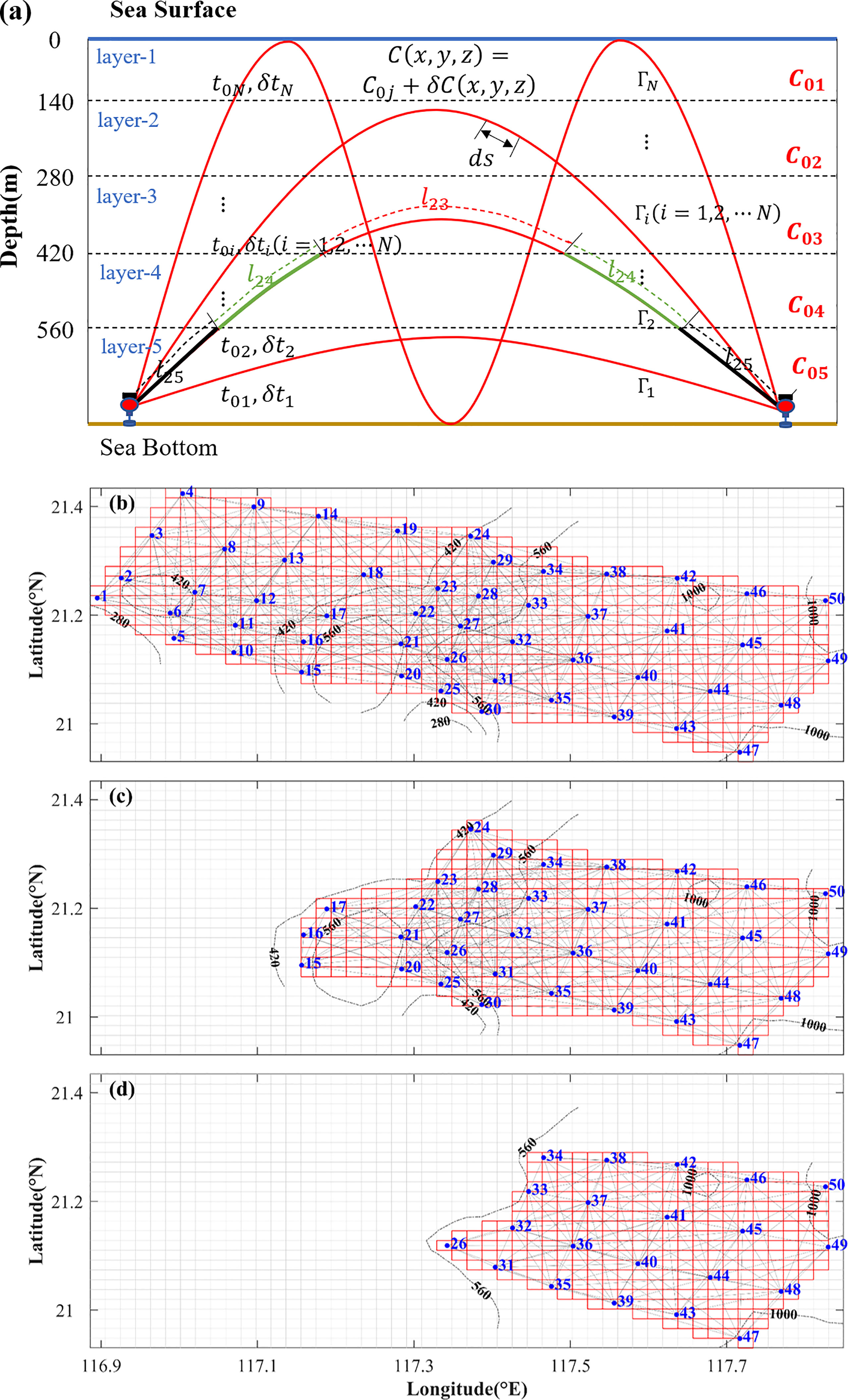
Figure 2 (A) Schematic diagram of the four refracted rays crossing the five layers in a vertical slice between two stations. C_0j and δCij(x,y,z) represent the reference sound speed and the sound speed deviation of the ith ray crossing jth layer, respectively.  l_ij is the arc length of the ith ray crossing the jth layer. t_0i and δt_i represent the reference travel time and the travel time deviation, respectively. (B) Maps of the virtual MCAT stations and the projected rays and grids for the horizontal-slice inversion in the first, second, and third layers. (C) Maps of the virtual MCAT stations and the projected rays and grids for the horizontal-slice inversion in the fourth layer. (D) Maps of the MCAT stations and the projected rays and grids for the horizontal-slice inversion in the fifth layer. The blue number denotes the station number and the gray lines denote the transmission paths between individual station pairs.

2.3. Ray simulation and determination of differential travel times

To simulate the acoustic transmission paths between each station pair, sound speed profiles were formed using temperature and salinity data from SUNTANS. Prior to vertical-slice inversion, it is needed to recognize two or more rays with different travel times at different depths. Thus, a vertical slice lying between the two stations was divided into multi-depth layers. A vertical slice with four rays and five depth layers is shown in Figure 2A.

According to the standard performance for sound propagation of the MCAT, it is assumed that reciprocal sound transmission is difficult between station pairs with a distance of > 25 km. Therefore, station pairs with distances of > 25 km were not considered in this simulation. As a result, 417 transmission paths were used in the 3D inversion of the sound speed. Figure 3 demonstrates an example of the simulated rays for one-way transmission from station C31 to C33 at hour 243 using the sound speed profiles between C31 and C33 (Figure 3A). In this case, there are four or five eigenray paths connecting two stations (Figure 3B). The rays arrived at the receiver within a time band of 10.793–11.198s (Figure 3C). Differential travel times were identified by the largest arrival peak method with the following steps: 1) because the time resolution for multi-arrival peaks of the M sequence (t_r = Q/f, where Q is 3 and f is 5 kHz here) is 0.6 ms, this value was set to the interval between the subsequent arrival peaks, 2) and signals with signal-to-noise ratios > 0.2 (Taniguchi and Huang, 2015) were considered (Figure 3D); and 3) during each interval, the largest arrival peak was selected (Figure 3D). Generally, 5 kHz was utilized in CAT studies. The primary objective of this paper is to discuss the feasibility of MCAT networking observations; the performances of different frequencies will be discussed in future work and are not tested here.

FIGURE 3

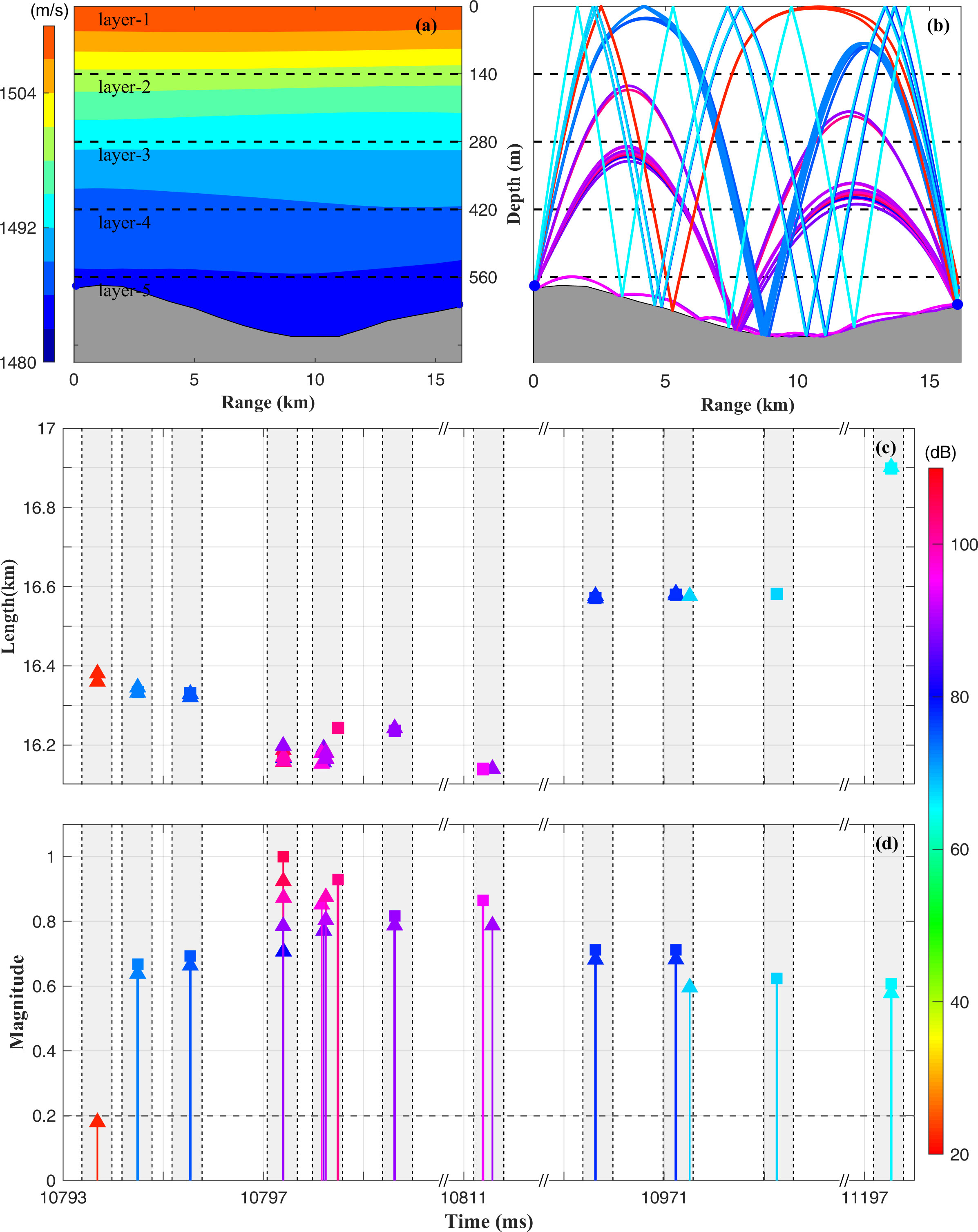
Figure 3 Ray simulation for the station pair C31–C33 at hour 243. (A) Contour map of the sound speed for the station pair C31–C33. (B) Eigenrays. (C) Ray arc length plotted against travel times. (D) Level of received sounds plotted against the travel time. The colors correspond to the sound level shown with color bar at the lower right. Shaded areas indicate the time bands for individual ray groups and the sound level is normalized using the maximum values.

Finally, station pairs of 416, 416, 416, 258, and 116 were selected for the first, second, third, fourth, and fifth layers, respectively (Table 1). Based on the upper rules for selecting the ray between each station pair, 1,637, 1,944, 2,387, 1,579, and 744 rays were selected for the first, second, third, fourth, and fifth layers, respectively (Table 1). The spatial resolutions in the first, second, third, fourth, and fifth layers were estimated to be approximately 2.7, 2.7, 2,7, 2.8, and 3.4 km ($\sqrt{A/N}$, where A is the area and N is the number of stations), respectively (Table 1). For each station pair, at least one ray runs through and the selected rays are distributed in each layer.

TABLE 1

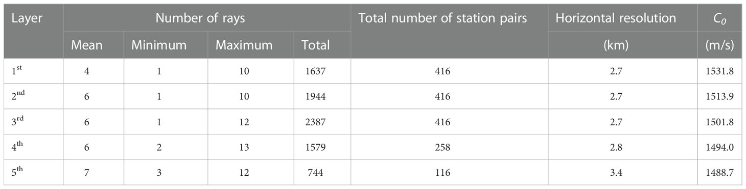
Table 1 Statistical factors of the eigenray between each station pair for each layer.

3. Inverse problem

3.1. Inversion on a vertical slice

In the MCAT experiment, reciprocal travel time data can be directly observed between each station pair. However, in this work, they were simulated along the acoustic ray path using the results of the SUNTANS model.

Following the vertical-slice inversion in Kaneko et al. (2020), as shown in Figure 2A, we present an example to demonstrate the vertical-slice inversion for four rays and five horizontal layers. Range-average sound speed deviations are considered unknown variables between each station pair, which are need to be solved by the vertical-slice inversion. In this study, one-way travel times were simulated, and the effect of velocity on them was neglected as a suitable assumption. The one-way travel time along each ray path Γ_i is calculated as follows:

$\begin{array}{ll}{t}_i={\displaystyle {\int }_{{\Gamma }_i}\frac{ds}{C_0\left(z\right)+\delta C\left(x,y,z\right)}}& (1)\end{array}$

where C₀(z) denotes the reference sound speed in each vertical layer, δC(x,y,z) denotes the sound speed deviation in the 3D (x, y, z) coordinate frame, and ds represents the increment in the arc length along the ray.

The one-way travel time along each ray in Figure 2A was calculated using the following equation:

$\begin{array}{ll}\{\begin{array}{c}\delta t_1=-\frac{l_{1,1}}{C_{0,1}^2}\Delta C_1-\frac{l_{1,2}}{C_{0,2}^2}\Delta C_2-\frac{l_{1,3}}{C_{0,3}^2}\Delta C_3-\frac{l_{1,4}}{C_{0,4}^2}\Delta C_4-\frac{l_{1,5}}{C_{0,5}^2}\Delta C_5\\ \delta t_2=-\frac{l_{2,1}}{C_{0,1}^2}\Delta C_1-\frac{l_{2,2}}{C_{0,2}^2}\Delta C_2-\frac{l_{2,3}}{C_{0,3}^2}\Delta C_3-\frac{l_{2,4}}{C_{0,4}^2}\Delta C_4-\frac{l_{2,5}}{C_{0,5}^2}\Delta C_5\\ \delta t_i=-\frac{l_{i,1}}{C_{0,1}^2}\Delta C_1-\frac{l_{i,2}}{C_{0,2}^2}\Delta C_2-\frac{l_{i,3}}{C_{0,3}^2}\Delta C_3-\frac{l_{i,4}}{C_{0,4}^2}\Delta C_4-\frac{l_{i,5}}{C_{0,5}^2}\Delta C_5\\ \delta t_N=-\frac{l_{N,1}}{C_{0,1}^2}\Delta C_1-\frac{l_{N,2}}{C_{0,2}^2}\Delta C_2-\frac{l_{N,3}}{C_{0,3}^2}\Delta C_3-\frac{l_{N,4}}{C_{0,4}^2}\Delta C_4-\frac{l_{N,5}}{C_{0,5}^2}\Delta C_5\end{array}& (2)\end{array}$

where δt_i (i=1,2⋯N) represents the acoustic travel time along the ith ray and C_0j and ΔC_j represent the reference sound speed and sound speed deviation in the jth layer, respectively.  l_ij is the arc length of the ith ray crossing the jth layer.

Eq. 2 can be written in the matrix form as follows:

$\begin{array}{ll}{y}_v=E_v{x}_v+n_{xv}& (3)\end{array}$

where y_v represents the vector of the sound speed deviation, E_v is the matrix obtained from the ray length and the reference sound speed, and n_xv represents the travel time error vector.

Eq. 4 constructs an ill-posed issue, and the regularized inversion scheme proposed by Rajan et al. (1987) was applied in this study. Then, the cost function is represented by

$\begin{array}{ll}{J}_v={\left(y_v-E_v{x}_v\right)}^T\left(y_v-E_v{x}_v\right)+{\lambda }_v{x}_v^T{H}_v^T{H}_v{x}_v& (4)\end{array}$

where superscript T means the transpose of the matrix. H_v is the regularization matrix constructed from a finite difference approximation of the second-order derivative operator s(x) and can be expressed as follows:

$\begin{array}{ll}S\left(x\right)={\displaystyle {\int }_{-D}^0{\left(\frac{{\partial }^{2}x}{\partial z^2}\right)}^{2}dz=\sum _{i=1}^M\frac{{\left(x_{i-1}-2x_i+x_{i+1}\right)}^2}{{\left(\Delta z\right)}^2}=\frac{x_v^T{H}_v^T{H}_v{x}_v}{{\left(\Delta z\right)}^2}}& (5)\end{array}$

In this work, Δz = 1 m, and then,

$\begin{array}{ll}{H}_v=\left[\begin{array}{ccccc}-2& 1& 0& 0& 0\\ 1& -2& 1& 0& 0\\ 0& 1& -2& 1& 0\\ 0& 0& 1& -2& 1\\ 0& 0& 0& 1& -2\end{array}\right]& (6)\end{array}$

By minimizing J_v , the optimal solution ${\overrightarrow{x}}_v$ reduces to

$\begin{array}{ll}{\overrightarrow{x}}_v={\left(E_v^T{E}_v+{\lambda }_v{H}_v^T{H}_v\right)}^{-1}{E}_v^T{y}_v& (7)\end{array}$

where λ_v is the Lagrange multiplier chosen using the L-curve method (O’Leary and Hansen, 1993).

3.2 Inversion on a horizontal slice

Horizontal-slice inversion rely on the results of the vertical-slice inversion. For the horizontal-slice inversion, in each layer, the tomography domain with 50 stations was segmented into numerous subdomains, as shown in Figures 2B–D. The rays and subdomains were numbered systematically for horizontal-slice inversion, the sound speed deviations are considered as unknown parameters. And the number of unknown parameters becomes M×N , M represents the grid numbers and N represents the ray number in each layer.

In the first, second, and third layers, M and N were considered as 776 and 417, respectively. Since the bathymetry becomes shallow in the west of the experimental area, for the fourth layer, M was 508 and N was 258, while for the fifth layer, M was 335 and N was 116 (Figure 2B–D). The one-way sound speed deviation is calculated as follows:

$\begin{array}{ll}\{\begin{array}{c}\Delta C_1=\frac{l_{1,1}}{l_1}\delta C_1+\frac{l_{1,2}}{l_1}\delta C_2+\cdots +\frac{l_{1,j}}{l_1}\delta C_j+\cdots +\frac{l_{1,M-1}}{l_1}\delta C_{M-1}+\frac{l_{1,M}}{l_1}\delta C_M\\ \Delta C_2=\frac{l_{2,1}}{l_2}\delta C_1+\frac{l_{2,2}}{l_2}\delta C_2+\cdots +\frac{l_{2,j}}{l_2}\delta C_j+\cdots +\frac{l_{2,M-1}}{l_2}\delta C_{M-1}+\frac{l_{2,M}}{l_2}\delta C_M\\ \Delta C_i=\frac{l_{i,1}}{l_i}\delta C_1+\frac{l_{i,2}}{l_i}\delta C_2+\cdots +\frac{l_{i,j}}{l_i}\delta C_j+\cdots +\frac{l_{i,M-1}}{l_i}\delta C_{M-1}+\frac{l_{i,M}}{l_i}\delta C_M\\ \Delta C_N=\frac{l_{N,1}}{l_N}\delta C_1+\frac{l_{N,2}}{l_N}\delta C_2+\cdots +\frac{l_{N,j}}{l_N}\delta C_j+\cdots +\frac{l_{N,M-1}}{l_N}\delta C_{M-1}+\frac{l_{N,M}}{l_N}\delta C_M\end{array}& (8)\end{array}$

where δC_j denotes the sound speed deviation for the jth subdomain and l_i,j denotes the length of the ith projected ray crossing the jth subdomain.

Similar to that in vertical inversion, equations 3, 4, 5, and 7 were also applied to horizontal inversion and were not introduced in detail here. The difference is H_h , which is the regularization matrix constructed from a finite difference approximation of the second-order derivative operator, that can be expressed as follows:

$\begin{array}{ll}{H}_h\left[\begin{array}{cccccccccc}-4& 1& 0& 1& 0& 0& 0& \cdots & 0& 0\\ 1& -4& 0& 0& 1& 0& 0& \cdots & 0& 0\\ 0& 0& -4& 1& 0& \cdots & 1& \cdots & \cdots & 0\\ 1& 0& 1& -4& 1& 0& \cdots & 1& \cdots & 0\\ ⋮& ⋮& ⋮& \ddots & ⋮& ⋮& ⋮& ⋮& ⋮& ⋮\\ 0& \cdots & 1& \cdots & 1& -4& 1& \cdots & 1& \cdots \\ ⋮& ⋮& ⋮& ⋮& ⋮& ⋮& \ddots & ⋮& ⋮& ⋮\\ 0& 0& 0& \cdots & 1& \cdots & 1& -4& 1& \cdots \\ 0& 0& 0& 0& \cdots & 1& \cdots & 1& -4& 1\\ 0& 0& 0& 0& 0& \cdots & 1& \cdots & 1& -4\end{array}\right]& (9)\end{array}$

4. Results of inverted 3D sound speed fields

4.1. Results of vertical inversion

The five-layer distributions of sound speed deviations between each station pair are shown in Figure 4. The values of sound speed deviation in the western area were higher than those in the eastern area (Figures 4A–F). The sound speed deviations in the first and second layers were almost uniform, and the difference between the western and eastern areas was< 0.5 m/s. The sound speed deviations in the third, fourth, and fifth layers showed an irregular distribution such that the sound speed deviations increased in the western part of the area. The results of the vertical-slice inversion were in good agreement with the results of the SUNTANS model (Figures 4A–F). Generally, the root-mean-square difference (RMSD) between the results of inversion and SUNTANS model are< 0.75 m/s (Figures 4K–O). Higher RMSDs (> 0.75 m/s) are mostly confined to the second layer and its edge. The RMSD was the lowest in the fifth layer, with a mean RMSD of 0.29 m/s.

FIGURE 4

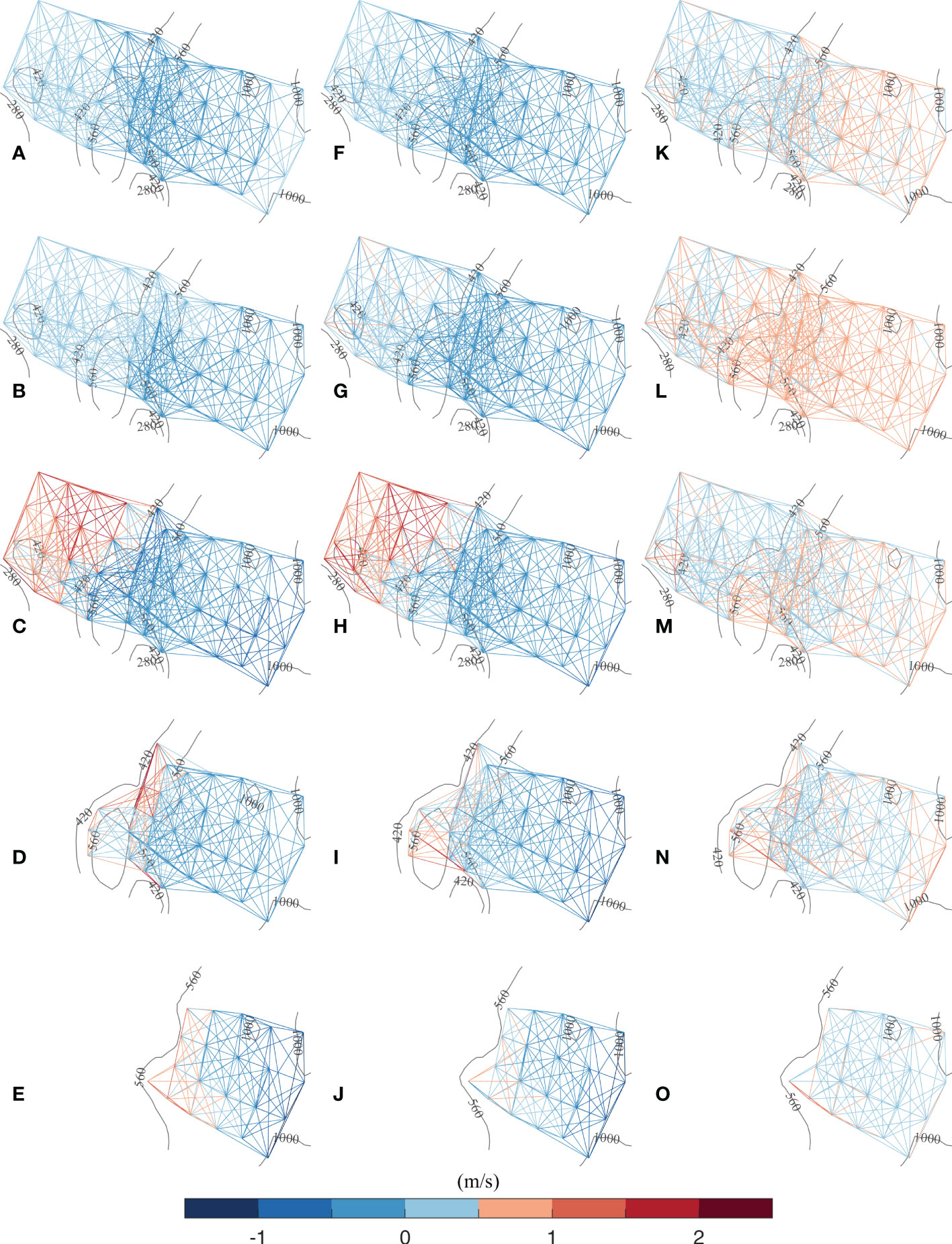
Figure 4 Results of the vertical-slice inversion. (A–E) Temporal plots of sound speed deviations calculated using the SUNTANS model along each transmission path. (F–J) Temporal plots of sound speed deviations derived from the vertical-slice inversion along each transmission path. (K–O) Temporal plots of RMSD calculated using the SUNTANS model and vertical-slice inversion. The first to fifth layers are from the top to bottom.

Because the second layer exhibited the most significant variations in sound speed deviation, the results of the SUNTANS model and vertical-slice inversion in the second layer were compared during one tidal cycle from hour 84 to hour 97 (Figure 5). The results of inversion were in good agreement with the results of the SUNTANS model, such that the locations of the high (low) sound-speed zones were coincident. From the above data, the high sound speed zones of > 1516 m/s were considered an index of internal tides, which took approximately 12 h to propagate from the eastern to western boundaries of the observation area, which is a distance of 93.1 km (Figure 5). This value resulted in a wavelength of 82.9 km and a phase speed of 1.9 m/s.

FIGURE 5

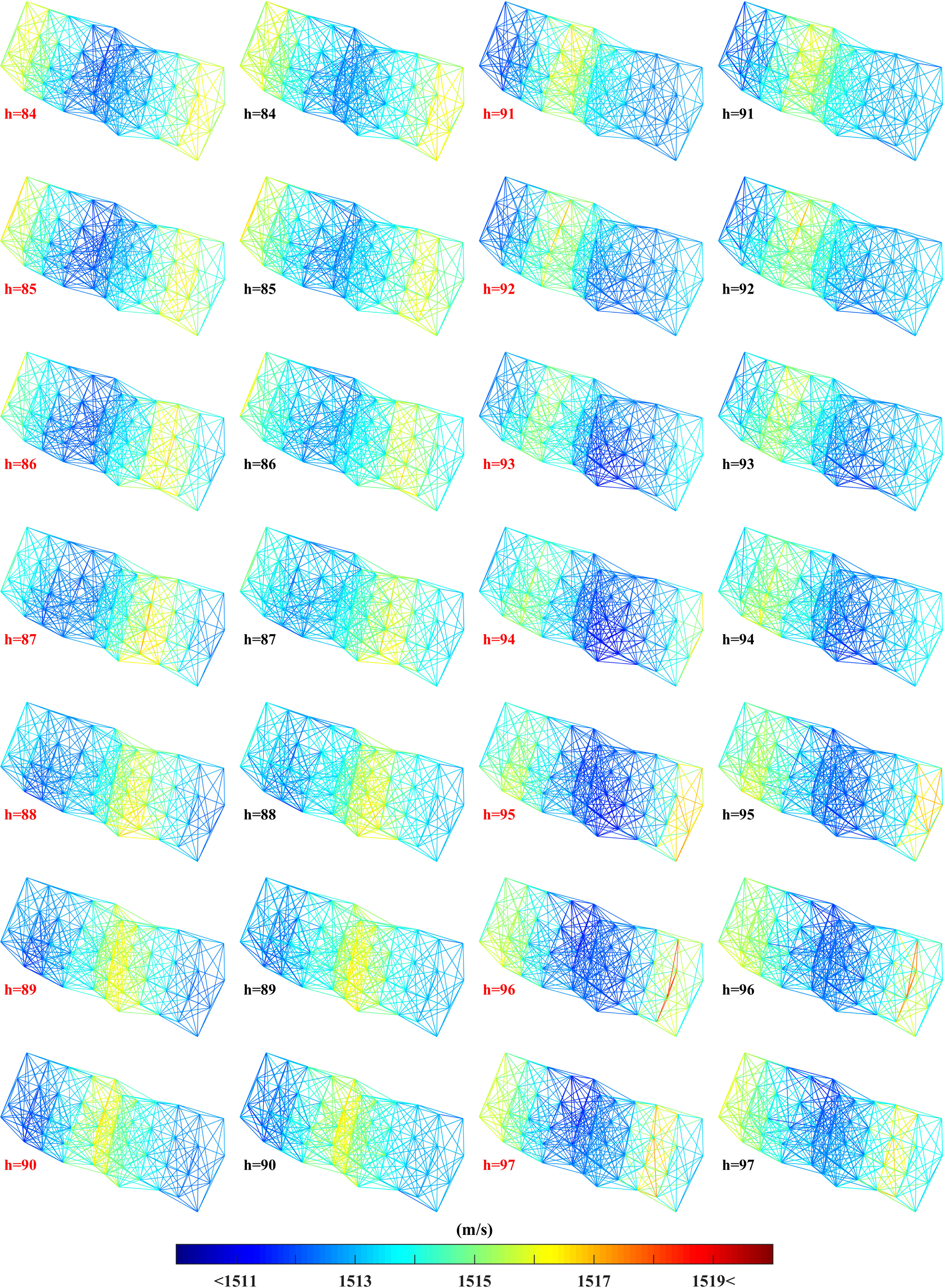
Figure 5 Results of vertical-slice inversion for the sound speed deviations calculated along each transmission path, during one tidal cycle from hour 84 to hour 97 in the second layer. The first and third columns are the results of the SUNTANS model, and the second and fourth columns are the results of vertical-slice inversion.

4.2. Results of horizontal inversion

The five-layer variations of the sound speed deviations are shown with contour plots in Figures 6A–E for the SUNTANS model, Figures 6F–J for vertical-slice inversion, and Figures 6K–O for the RMSDs of both data. For both datasets, the values of sound speed deviations were higher in the western area than in the eastern area. In the first and second layers, the differences between the western and eastern areas were approximately 0.5 m/s, whereas in the third, fourth, and fifth layers, the difference was approximately 1.5 m/s. The main reason for this increase is the variation in bathymetry in the observation area, wherein the effects of the continental slope became significant in the third, fourth, and fifth layers. The results of horizontal-slice inversion are in good agreement with those of the SUNTANS model. The RMSDs for each layer were< 1.0 m/s. Higher RMSDs (> 1.25 m/s) appeared at the western edge of the third and fourth layer, which were mostly caused by the sparse distribution of transmission paths and the complicated bathymetry.

FIGURE 6

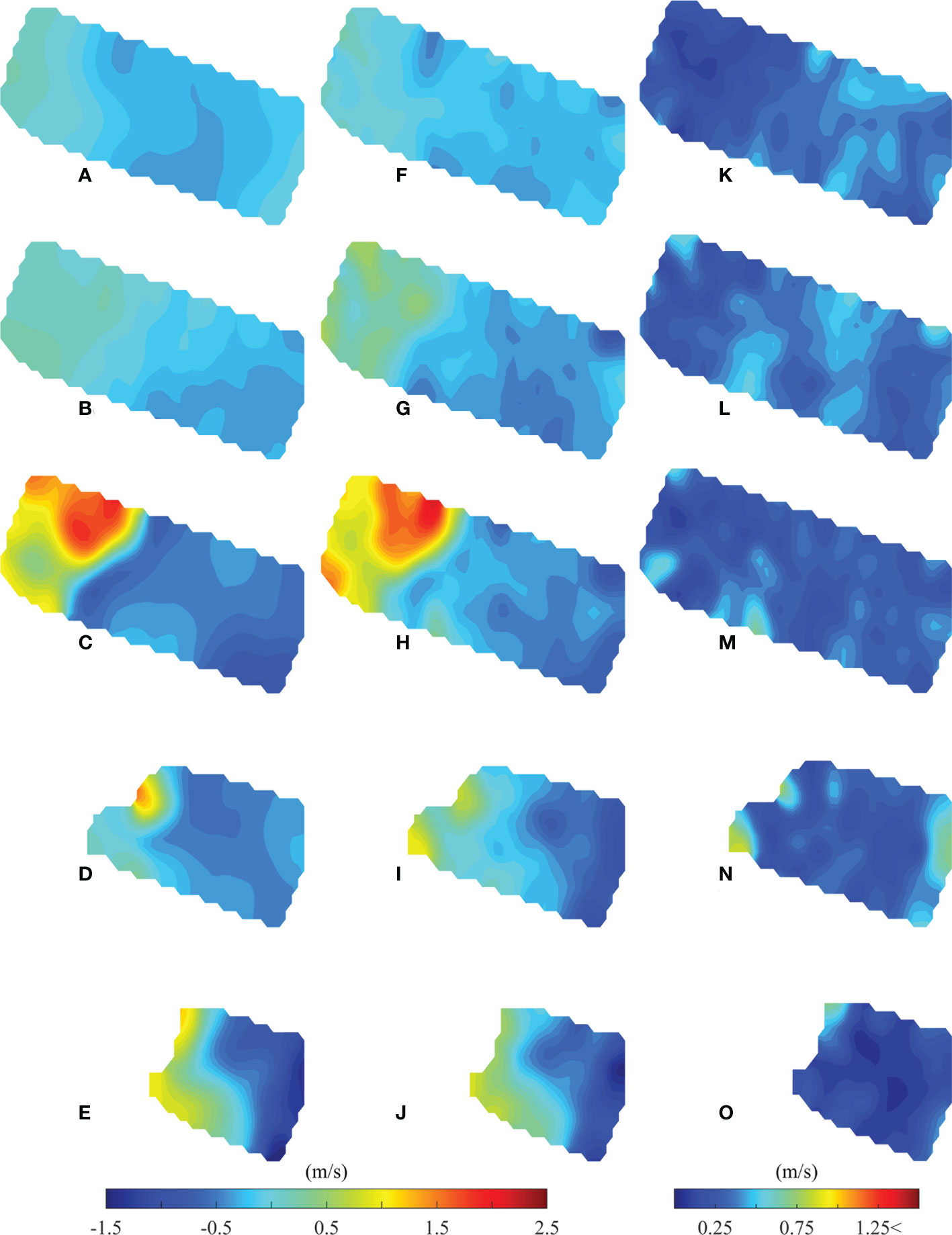
Figure 6 Results of the horizontal-slice inversion for sound speed deviations. (A–E) Temporal plots of sound speed deviation fields calculated using the SUNTANS model in each layer. (F–J) Temporal plots of sound speed deviation fields calculated from the horizontal-slice inversion in each layer. (K–O) Temporal plots of RMSDs calculated using the SUNTANS model and horizontal-slice inversions. The first to fifth layers are from the top to bottom.

The results of the SUNTANS model and horizontal-slice inversion for sound speed in the second layer are shown as contour plots during one tidal cycle from hour 84 to hour 97 in Figure 7. The first and third columns of the figure are for the SUNTANS model, and the second and fourth columns are for the horizontal-slice inversion. The distributions of the large sound speed zones confined to the western area showed good agreement between the SUNTANS model and horizontal-slice inversion. The wavelength and phase speed values of internal tides calculated from the horizontal-slice inversion are similar to the vertical inversion results. The high sound speed zone transmits with a phase speed of 1.9 m/s from the east boundary to the west boundary.

FIGURE 7

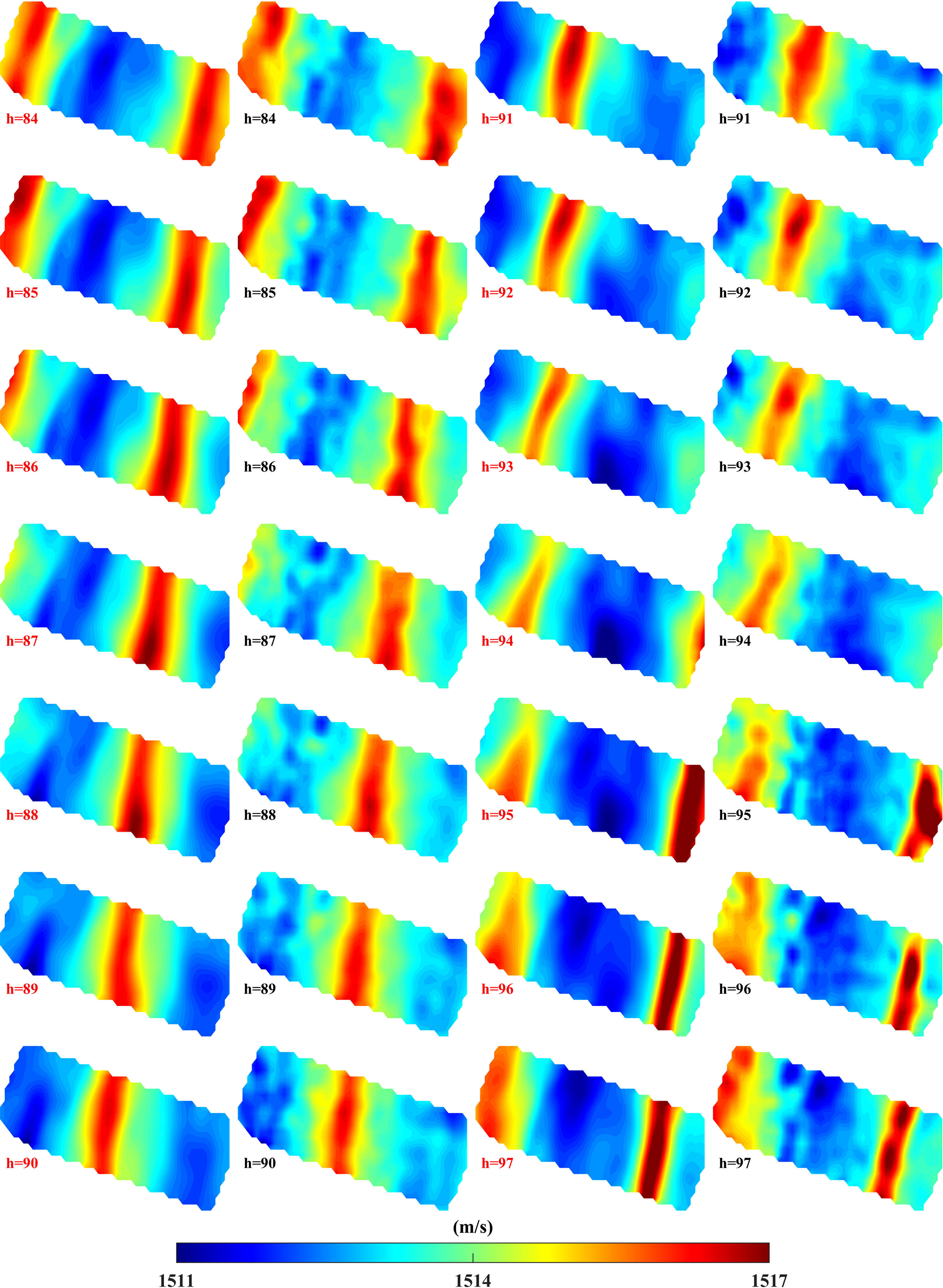
Figure 7 Results of the horizontal-slice inversion for sound speed during one tidal cycle from hour 84 to hour 97 in the second layer. The first and third columns are the results of the SUNTANS model and the second and fourth columns are results of the horizontal-slice inversion.

5. Discussion on potential influencing factors

5.1. Swing of the anchor tether

Positioning errors are the most critical factors in sound-speed inversion. The swing of the moored MCAT system is a significant source of positioning error. Hence, a numerical experiment was conducted to evaluate the positioning error, which mostly results from the swing of the anchor tether. This study demonstrated the use of MCAT network observation in monitoring internal tides using sound speed. Generally, MCAT is deployed close to the bottom with an anchor, and it is set to approximately 5 m above the seafloor using a float. The results of the sensitivity experiment using a 5-m random swing are shown with the contour plot of sound speed deviations in Figure 8. Figure 8A represents the sound speed deviation obtained using the SUNTANS model. Figure 8B represents the results of the second-layer inversion with 0 m drift at hour 92. Both data showed good agreement, wherein the zone of higher values related to internal tides was coincident. Figure 8C shows the results of inversion, considering the 5-m random swing of the MCAT system, which is mostly generated by an oceanographic phenomenon (e.g., internal tide) (Figure 8D). The swing was random, although there are some differences in the results of inversion, the inversion errors are< 1.0 m/s (Figure 8C). Even though the moored MCAT would have some swing in the anchor tether, it did not affect its ability to capture the propagation processes of internal tides, suggesting the feasibility of using observations of the MCAT network to monitor internal tides.

FIGURE 8

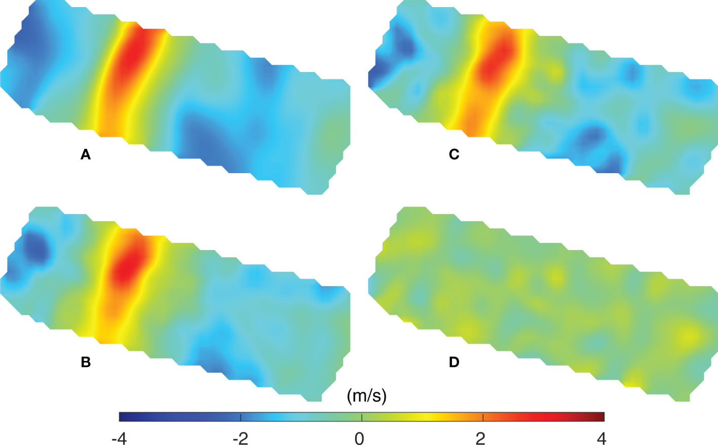
Figure 8 Distributions of the sound speed deviation at hour 92 from (A) SUNTANS, (B) inversion with no distance drift, (C) inversion with the addition of the random 5-m drift, and (D) distribution of sound speed deviations that resulted from the random 5-m drift.

5.2. Movement of the anchor mooring position

The accuracy of the results of inversion was significantly influenced by the positional movement of the acoustic stations. One sensitivity experiment was conducted to evaluate the effect of the movement of stations exerted by human activities on the results of inversion. Specifically, we suppose that a station is moved due to fishing activities and discuss how much the movement of one specific station affects the MCAT network observation of the entire area. As shown in Figure 9, the station movement was considered in various directions from the internal tide propagation (16° north to west). As the distance of movement increased in a specific direction, inversion error increased. Although a 10-m movement resulted in a maximum error of 1.1 m/s (Figure 9D), the effect on the network observation was weak and did not have a significant impact on the observation of internal tides (Figures 9A, D). When the distance of movement was 50 m, the inversion error reached 5.9 m/s and the area of influence was limited. Furthermore, a distance of movement of 100 m caused an error of approximately 11.9 m/s. As a result, internal tides could no longer be monitored well (Figures 9B, C, E, F).

FIGURE 9

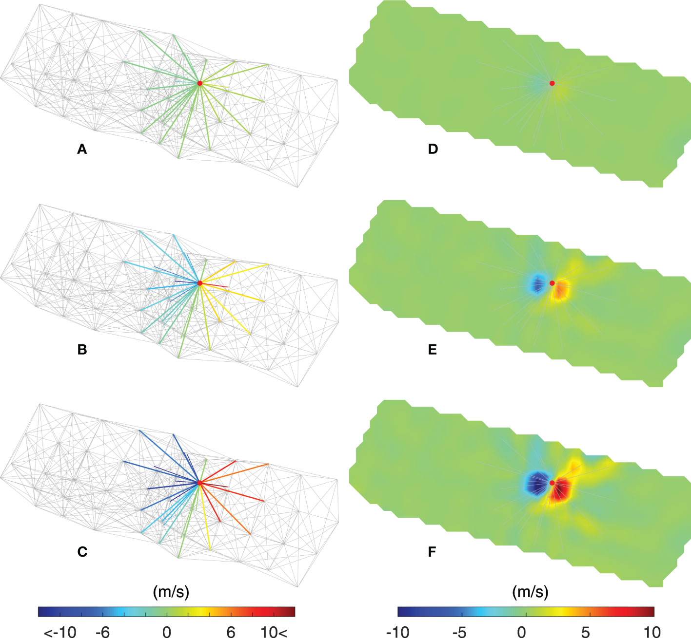
Figure 9 Results of the sensitivity experiments for station movement at hour 92. (A–C) Sound speed deviations generated by station movements of 10, 50, and 100 m at a specific station in the middle of the network area. The transmission lines marked with color represent the station pairs that are influenced by the movement of the station. The station is moved from east to west. (D–F) Inversion errors generated by the station movement of 10, 50, and 100 m at a specific station in the middle of the network area. The transmission lines represent the station pairs that are influenced by the movement of the station.

5.3. System missing

Numerous MCATs were deployed to construct a network observation to confirm the possibility of monitoring internal tides. Hence, if unexpected troubles occur at one or several stations (e.g., lost or unable to transmit sound), we must ascertain their quantum of influence in monitoring internal tides via inversion. The effects generated by the missing MCAT stations are the focus of this study. As shown in Figure 10, four sensitivity experiments with different missing position arrangements were conducted to examine the effects on the results of inversion. When only one station located at the boundary is missing, the error was low with a maximum of 0.26 m/s. Besides, the associated missing rays lead to several subdomains without rays through the grids for horizontal inversion, thus decreasing the monitoring area (Figures 10A, E). Different from the aforementioned case, if the missing station was located inside the network with no missing subdomains, inversion errors were even lesser, with a maximum of 0.22 m/s (Figures 10B, F). In the case of two missing stations, the inversion error increased and the maximum error was< 0.50 m/s (Figures 10C, D, G, H), and the overall feature of internal tides was still reconstructed as their sound speed variations reached up to 6 m/s (see Figures 5, 7).

FIGURE 10

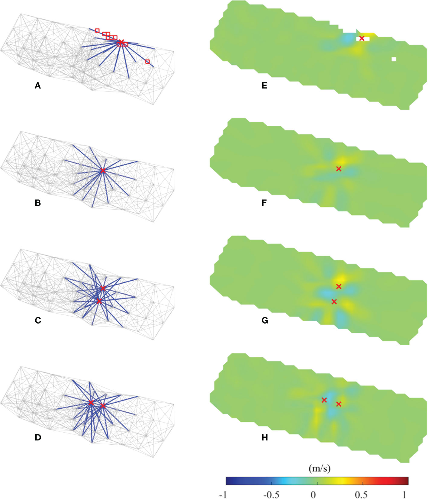
Figure 10 Results of the sensitivity experiments of missing stations in the network at hour 92. (A–D) The cross sign demonstrates the position of the missing station; the blue lines represent the transmission paths related to the missing station. (E–H) Inversion error generated by missing stations. The red cross marks indicate the positions of missing station. The red squares in (A) indicate the missing subdomains induced by the missing station, and the white squares in (E) match the red squares.

5.4. Clock drift

MCAT is equipped with a chip-scale atomic clock (CSAC), which is the lowest-power and lowest-profile atomic clock in the world, to capture the high-resolution of time. With a typical aging rate of 9 × 10⁻¹⁰/s Hz/Hz (White Paper, 2018), the CSAC has a fairly good frequency drift (and corresponding time error). Taking the results of its derivation, the timing error accumulation over one month is 2.4 ms. Considering the time error generated by both drifts for one year of observation, the inversion errors resulting from the clock drift are as low as 0.5 m/s. The errors did not significantly influence the results of inversion because the sound speed variations related to the internal tides reached up to 6 m/s (see Figures 5, 7).

5. Conclusions

We examined the effectiveness of the network observation using 50 MCATs in a complicated deep-sea environment via numerical simulations using the synthetic ocean output obtained using the SUNTANS model. The considered cases were adequate to demonstrate the applicability of the network observation to tomographic mapping of sound speed fields in complicated deep-sea environments to capture the propagation of internal tides. The 3D fields of the sound speed inside the observation area were reproduced well in a sequence of vertical- and horizontal-slice inversions. Although some differences existed, the inverted sound speed fields showed good agreement with data of the SUNTANS model. The RMSD values of sound speeds obtained by the inversion and SUNTANS models were< 1.0 m/s. The locations of the higher sound speed zones generated by internal tides were coincident between the inversion result and the SUNTANS model. Sensitivity experiments involving the movement of the MCAT stations showed that a distance of movement of< 5 m, which is mostly caused by the swing of the anchor tether, had a low effect on the results of inversion. Large movements over 50 m, which resulted from the movement of stations, no longer served to observe sound speed variations due to internal tides. The sensitivity experiments of missing stations showed that although the error increased with two missing stations, the maximum error was still at an acceptable level of< 0.5 m/s.

The higher sound speed zone generated by internal tides was captured well by the 3D inversion of the simulated MCAT data. MCAT is an advanced system of traditional CAT with a mirror forwarding function that transmits offshore observation data to the nearshore. These results suggest that MCAT network observation using numerous stations are the most efficient in capturing the propagation of internal tides. In this study, mirror function was not implemented in the SCS, and only simulation results were provided; therefore, in future studies, mirror function will be addressed, and the application of MCAT to monitor internal tides in the SCS will be determined.

Data availability statement

The original contributions presented in the study are included in the article/supplementary material. Further inquiries can be directed to the corresponding author.

Author contributions

LD and X-HZ contributed to conception and design of the study. LD and CX performed the statistical analysis. CX, X-HZ, Z-NZ and HZ wrote the first draft of the article. Z-NZ, CZ, and QL organized the data. All authors contributed to article revision, read, and approved the submitted version.

Funding

This research was funded by the National Natural Science Foundation of China (grants 41920104006, 52071293), the Scientific Research Fund of the Second Institute of Oceanography, MNR (JZ2001), the National Key Research and Development Program of China (2021YFC3101502), the Project of State Key Laboratory of Satellite Ocean Environment Dynamics, Second Institute of Oceanography (SOEDZZ2207 and SOEDZZ2106), the Oceanic Interdisciplinary Program of Shanghai Jiao Tong University (project number SL2021MS021), and the Innovation Group Project of the Southern Marine Science and Engineering Guangdong Laboratory, Zhuhai (No. 311020004).

Conflict of interest

The authors declare that the research was conducted in the absence of any commercial or financial relationships that could be construed as a potential conflict of interest.

Publisher’s note

All claims expressed in this article are solely those of the authors and do not necessarily represent those of their affiliated organizations, or those of the publisher, the editors and the reviewers. Any product that may be evaluated in this article, or claim that may be made by its manufacturer, is not guaranteed or endorsed by the publisher.

References

Buijsman M. C., Kanarska Y., McWilliams J. C. (2010). On the generation and evolution of nonlinear internal waves in the south China Sea. J. Geophys. Res. Ocean. 115, 1–17. doi: 10.1029/2009JC005275

CrossRef Full Text | Google Scholar

Chen M, Kaneko A, Lin J, Zhang C. (2017). Mapping of a Typhoon-Driven Coastal Upwelling by Assimilating Coastal Acoustic Tomography Data. J. Geophys. Res. Ocean. 122, 7822–7837. doi: 10.1002/2017JC012812

CrossRef Full Text | Google Scholar

Chen M., Syamsudin F., Kaneko A., Gohda N., Howe B. M., Mutsuda H., et al. (2018). Real-time offshore coastal acoustic tomography enabled with mirror-transpond functionality. IEEE J. Ocean. Eng. 45, 645–655. doi: 10.1109/JOE.2018.2878260

CrossRef Full Text | Google Scholar

Cornuelle B., Munk W., Worcester P. (1989). Ocean acoustic tomography from ships. J. Geophys. Res. Ocean. 94, 6232–6250. doi: 10.1029/JC094iC05p06232

CrossRef Full Text | Google Scholar

Fringer O. B., Gerritsen M., Street R. L. (2006). An unstructured-grid, finite-volume, nonhydrostatic, parallel coastal ocean simulator. Ocean Model. 14, 139–173. doi: 10.1016/j.ocemod.2006.03.006

CrossRef Full Text | Google Scholar

Kaneko A., Zhu X.-H., Lin J. (2020). Coastal acoustic tomography (Amsterdam, Netherlands: Elsevier). doi: 10.1016/B978-0-12-818507-0.00003-2

CrossRef Full Text | Google Scholar

Li Q., Farmer D. M. (2011). The generation and evolution of nonlinear internal waves in the deep basin of the south China Sea. J. Phys. Oceanogr. 41, 1345–1363. doi: 10.1175/2011JPO4587.1

CrossRef Full Text | Google Scholar

O’Leary D. P., Hansen P. C. (1993). The use of the l-curve in the regularization of discrete ill-posed problems. SIAM J. Sci. Comput. 14, 1487–1503. doi: 10.1137/0914086

CrossRef Full Text | Google Scholar

Park JH, Kaneko A. (2001). Computer simulation of coastal acoustic tomography by a two-dimensional vortex model. Journal of oceanography 57, 593–602. doi: 10.1023/A:1021211820885

CrossRef Full Text | Google Scholar

Porter M. B. (2011). The bellhop manual and user’s guide: Preliminary draft. heat. doi: 10.1038/299121a0

CrossRef Full Text | Google Scholar

Rajan S. D., Lynch J. F., Frisk G. V. (1987). Perturbative inversion methods for obtaining bottom geoacoustic parameters in shallow water. J. Acoust. Soc Am. 82, 998–1017. doi: 10.1121/1.395300

CrossRef Full Text | Google Scholar

Send U., Schott F., Gaillard F., Desaubies Y. (1995). Observation of a deep convection regime with acoustic tomography. J. Geophys. Res. Ocean. 100, 6927–6941. doi: 10.1029/94JC03311

CrossRef Full Text | Google Scholar

Syamsudin F., Taniguchi N., Zhang C., Hanifa A. D., Li G., Chen M., et al. (2019). Observing internal solitary waves in the lombok strait by coastal acoustic tomography. Geophys. Res. Lett. 46, 10475–10483. doi: 10.1029/2019GL084595

CrossRef Full Text | Google Scholar

Taniguchi N., Huang C. F. (2015). Simulated tomographic reconstruction of ocean current profiles in a bottom-limited sound channel. J. Geophys. Res. Ocean. 119, 4999–5016. doi: 10.1002/2014JC009885

CrossRef Full Text | Google Scholar

The Ocean Tomography Group. (1982). A demonstration of ocean acoustic tomography. Nature 299, 121–125. doi: 10.1038/299121a0

CrossRef Full Text | Google Scholar

White Paper (2018). Chip-scale atomic clock (CSAC) performance during rapid chip-scale atomic clock (CSAC) performance during rapid temperature. (Aliso Viejo, USA).

Google Scholar

Worcester P. F., Lynch J. F., Morawitz W. M. L., Pawlowicz R., Sutton P. J., Cornuelle B. D., et al. (1993). Evolution of the large-scale temperature field in the Greenland Sea during 1988-89 from tomographic measurements. Geophys. Res. Lett. 20, 2211–2214. doi: 10.1029/93GL02373

CrossRef Full Text | Google Scholar

Wunsch M. C. (1979). Ocean acoustic tomography: A scheme for large scale monitoring. Deep Sea Res. Part A. Oceanogr. Res. Pap 26, 123–161. doi: 10.1016/0198-0149(79)90073-6

CrossRef Full Text | Google Scholar

Yamaguchi K., Lin J., Kaneko A., Yayamoto T., Gohda N., Nguyen H. Q., et al. (2005). A continuous mapping of tidal current structures in the kanmon strait. J. Oceanogr. 61, 283–294. doi: 10.1007/s10872-005-0038-y

CrossRef Full Text | Google Scholar

Yamoaka H., Kaneko A., Park J. H., Hong Z., Gohda N., Takano T., et al. (2002). Coastal acoustic tomography system and its field application. IEEE J. Ocean. Eng. 27, 283–295. doi: 10.1109/JOE.2002.1002483

CrossRef Full Text | Google Scholar

Yuan G., Nakano I., Fujimori H., Nakamura T., Kamoshida T., Kaya A. (1999). Tomographic measurements of the kuroshio extension meander and its associated eddies. Geophys. Res. Lett. 26, 79–82. doi: 10.1029/1998GL900253

CrossRef Full Text | Google Scholar

Zhang Z., And O., Ramp S. R. (2011). Three-dimensional, nonhydrostatic numerical simulation of nonlinear internal wave generation and propagation in the south China Sea. J. Geophys. Res. Ocean 116, 1–26. doi: 10.1029/2010JC006424

CrossRef Full Text | Google Scholar

Zhang C., Kaneko A., Zhu X. H., Gohda N. (2015). Tomographic mapping of a coastal upwelling and the associated diurnal internal tides in Hiroshima bay, Japan. J. Geophys. Res. Ocean. 120, 4288–4305. doi: 10.1002/2014JC010676

CrossRef Full Text | Google Scholar

Zhao Z. (2015). Internal tide radiation from the Luzon strait. J. Geophys. Res. Ocean. 119, 5434–5448. doi: 10.1002/2014JC010014

CrossRef Full Text | Google Scholar

Zhao Z., Alford M. H., Mackinnon J. A., Pinkel R. (2010). Long-range propagation of the semidiurnal internal tide from the Hawaiian ridge. J. Phys. Oceanogr. 40, 713–736. doi: 10.1175/2009JPO4207.1

CrossRef Full Text | Google Scholar

Zheng H., Gohda N., Noguchi H., Ito T., Yamaoka H., Tamura T., et al. (1997). Reciprocal sound transmission experiment for current measurement in the seto inland Sea, Japan. J. Oceanogr. 53, 117–128.

Google Scholar

Zheng H., Yamaoka H., Gohda N., Noguchi H., Kaneko A. (1998). Design of the acoustic tomography system for velocity measurement with an application to the coastal sea. J. Acoust. Soc Japan 19, 199–210. doi: 10.1250/ast.19.199

CrossRef Full Text | Google Scholar

Zhu X. H., Kaneko A., Wu Q., Zhang C., Taniguchi N., Gohda N. (2013). Mapping tidal current structures in zhitouyang bay, China, using coastal acoustic tomography. IEEE J. Ocean. Eng. 38, 285–296. doi: 10.1109/JOE.2012.2223911

CrossRef Full Text | Google Scholar

Zhu Z., Zhu X., Guo X., Fan X., Zhang C. (2017). Assimilation of coastal acoustic tomography data using an unstructured triangular grid ocean model for water with complex coastlines and islands. J. Geophys. Res. Ocean. 122, 7013–7030. doi: 10.1002/2017JC012715

CrossRef Full Text | Google Scholar