 Jiayuan Chen1,2
 Zifeng Hu2,3,4*
- 1School of Cyber Science and Technology, Sun Yat-sen University & Southern Marine Science and Engineering Guangdong Laboratory (Zhuhai), Zhuhai, China
- 2School of Marine Sciences, Sun Yat-sen University, Zhuhai, China
- 3Pearl River Estuary Marine Ecosystem Research Station, Ministry of Education, Zhuhai, China
- 4Guangdong Provincial Key Laboratory of Marine Resources and Coastal Engineering, Zhuhai, China
Ubiquitous fronts are a key part of energy transfer from large scales to small scales and exert a great impact on material exchange and biogeochemical processes. The spatial pattern and seasonal variability of cold- and warm fronts over the wide shelf of the northern South China Sea (SCS) are investigated using a 20-year time series (2002−2021) of 1-km spatial resolution Group for High Resolution Sea Surface Temperature (GHRSST) images. Our analysis shows distinct spatial and temporal variability in the occurrence of the cold- and warm fronts. Over the inner shelf (depth <50 m), the band-shaped cold fronts are predominately observed during spring through autumn from east of Hainan Island to Taiwan Shoal, with the presence of the maximum intensity and probability in winter. The frontal formations are possibly associated with the joint effect of the Guangdong Coastal Current (GCC) and the South China Sea Warm Current. During summer, the inshore fronts have relatively low probability and gradient magnitude. The warm fronts mainly occur off the western Guangdong coast possibly due to the southwestward-flowing GCC, whereas the cold fronts dominate off the eastern Guangdong coast and the eastern Hainan Island largely because of the coastal upwelling. Over the outer shelf (depth >50 m), the finer-scale cold- and warm fronts are discretely observed, with relatively weaker intensity and lower probability. The frontal activities are very vigorous in winter but slightly quiescent in summer, apparently resulting from the influence of the rich submesoscale processes in the SCS. This study could help improve our understanding of the SCS oceanic multiscale dynamics.
Introduction
Fronts in the ocean are the junction of different water masses and the narrow transition zones with relatively obvious changes in physical, biological, and/or chemical properties (Legeckis, 1978). Oceanic fronts are ubiquitous, with spatial scales ranging from O(1) to O(1000) km (Fedorov, 1986). The front dynamics are very active, where the energy transfers strongly from large scale to small scale, accompanied by the generation of internal waves, intense turbulence and upwelling, etc. (Chu and Wang, 2003). Strong material exchange induced by fronts could bring deep nutritive water to the upper layer, thereby enhancing local biological productivity (Fournier, 1978). Understanding the oceanic fronts and their variability is therefore essential for studying multiscale ocean dynamics, marine ecosystems and fishery productivity (Wang et al., 2020).
The South China Sea (SCS) is the largest marginal sea in the Western Pacific. It connects to the East China Sea and the Pacific Ocean by the Taiwan and Luzon Channels (Ren et al., 2015; Hu et al., 2016). Under the impact of seasonally varying monsoon, Kuroshio intrusion, and complex bathymetry (Liu et al., 2002; Qu et al., 2007), various fronts exist in the SCS and show pronounced spatiotemporal variability. Using hourly infrared satellite cloud maps, Chen (1983) explored the distribution of fronts in the northern South China Sea (NSCS) in winter. Using multi-year monthly sea surface temperature (SST) satellite data in the NSCS, Wang et al. (2001) analyzed the location and seasonal variability of several major fronts by calculating the frequency of frontal occurrences. Yao et al. (2012) used a visual graphical method to describe the monthly fronts in the entire SCS (Chen et al., 2012; Wang et al., 2012; Guo et al., 2017). Using 4-km spatial resolution SST satellite observations, Wang et al. (2020) identified wind-related fronts near the coast of northern Luzon and Vietnam.
Oceanic cold- and warm fronts were originally introduced by Ullman and Cornillon (1999). They presented the spatial pattern and temporal variability of cold- and warm fronts off the northeast U.S. coast. Based on local bathymetry and temperature gradients, Ullman and Cornillon (2001) further developed more detailed algorithms for distinguishing warm and cold fronts. Lately, Chang et al. (2008) explored the relationship between cold- and warm fronts in the East China Sea and chlorophyll-a concentration. However, the identification of cold- and warm fronts and the corresponding variations in the SCS have not yet been investigated for the present.
The main objectives of this study are to present a basic overview of the cold- and warm fronts in the NSCS, and to describe the seasonal cycle in the occurrence and strength of these fronts, based on the 1-km spatial resolution GHRSST (Group for High Resolution Sea Surface Temperature) SST data over a span of 20-year period (2002-2021). The paper is organized as follows: Section 2 describes the data and methods; Section 3 shows the mean seasonal cycle of the cold- and warm fronts over the NSCS shelf. Discussion and conclusions are given in section 4.
Data and methods
Study area
The area of interest for this study is a portion of the NSCS (108°-121°E, 17°-24°N), extending from the east coast of Hainan Island to the Taiwan Shoal. To subsequently present the front occurrence statistics, the study region has been subdivided into three sub-areas shown in Figure 1. The chosen boundaries are partly based on bathymetric and geographic features, e.g., the shelfbreaks, the Pearl River Estuary (PRE), and the Kuroshio-influenced Taiwan Shoal (Ren et al., 2015; Yu et al., 2020).
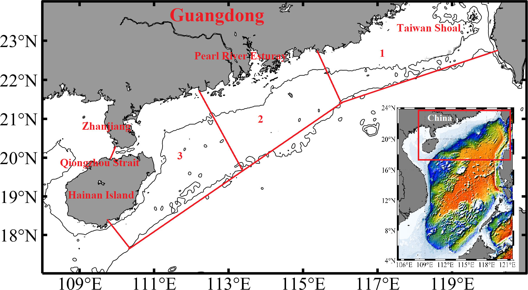
Figure 1 Bathymetry of the northern South China Sea (NSCS). Black contours indicate 50-m and 200-m isobaths. The study region is subdivided into three shelf zones (red lines) for subsequent analysis.
Data
The daily SST data from June 2002 to December 2021 are derived from the Group for High-Resolution Sea Surface Temperature (GHRSST) project based on several instruments, e.g., the NASA Advanced Microwave Scanning Radiometer-EOS (AMSR-E), the JAXA Advanced Microwave Scanning Radiometer 2 on GCOM-W1, the Moderate Resolution Imaging Spectroradiometers (MODIS) on the NASA Aqua and Terra platforms, the US Navy microwave WindSat radiometer, the Advanced Very High-Resolution Radiometer (AVHRR) on several NOAA satellites, and in situ SST observations from the NOAA iQuam project. The GHRSST data have a 1-km spatial resolution and are obtained from NASA’s Physical Oceanography Distributed Active Archive Center (PO.DAAC) (https://podaac.jpl.nasa.gov/dataset).
SST front detection
An objective edge detection technique based on Jensen-Shannon divergence (JSD), called entropy-based algorithm, was proposed by Shimada et al. (2005) and used to identify surface thermal fronts. The method has independence from spatiotemporal varying geophysical parameters and shows better performance compared with other conventional methods [e.g., gradient magnitude and histogram edge detection algorithm) (Shimada et al., 2005; Chang and Cornillon, 2015; Hu et al., 2021). Specifically, four different JSD matrices are firstly calculated in each of two 5×5 pixel SST subwindows with four different directions (horizontal, vertical, and two diagonals, see Shimada et al. (2005)]. The final JSD value at each pixel is assigned with the maximum of the four JSD matrices. It ranges from zero to one and represents the spatial inhomogeneity of two neighboring SST subwindows across a front. Stronger fronts have higher JSD values. To detect more and finer-scale fronts, JSD≥0.4 in this study is used as a frontal pixel.
At subinertial time scales, it is anticipated that the flow associated with a density front is roughly be in geostrophic balance, with the flow primarily in the along-front direction. The orientation of the SST front reveals the direction of the along-front subinertial flow if SST fronts are supposed to have a density signature. The temperature gradient vector’s direction, averaged along the length of the front, is assumed to be the direction of the mean frontal orientation (Ullman and Cornillon, 2001). Following Ullman and Cornillon (2001), the orientation of a front relative to the local bathymetry is measured by the normalized scalar product of the SST gradient and bathymetry gradient vectors. The normalized scalar product P is calculated with the formula:
where T is the SST and H is the water depth. The P-value ranges from −1 to 1. When the front is parallel to the local isobath, P-value reaches the minimum (maximum) which corresponds to cold (warm) water on the shallow side. When P-value is zero, the front is perpendicular to the local isobath. The P domain is then classified into three ranges (Figure 2): cold fronts (−1≤P≤−0.6), warm fronts (0.6≤P ≤ 1), and cross-isobath fronts (−0.6<P<0.6).

Figure 2 A schematic diagram illustrates the relationship between the P value and the classification of warm and cold fronts.
Frontal probability (FP) at each pixel (Ullman and Cornillon, 1999; Shimada et al., 2005) is defined as follows:
where Nfront is the number of valid frontal pixels with JSD≥0.4, Nvalid is the number of total valid pixels over 20 years. FP represents the mean probability of a front passing through a pixel.
The SST frontal gradient magnitude (GM), a measure of frontal strength, is defined as:
where ∂T/∂x and ∂T/∂y correspond to the gradient magnitudes in x and y directions. Frontal gradient direction is the angle between frontal gradient vector and due north direction. The cross-front length L, another measure of frontal strength, is calculated by the following formula (Ullman and Cornillon, 2001):
where ∆T is the mean cross-front temperature step and ∇T is the mean cross-front temperature gradient.
Results
Seasonal SST variability
Seasonal SST variability is briefly described for setting the stage for the discussion of the seasonal cycle in front occurrence. Figure 3 shows the seasonal SST averaged over 2002-2021, illustrating the differences between winter, spring, summer, and autumn SST patterns. In winter, the isotherms over the shelf are roughly parallel to the coast, and a band of cold water (< 21°C) is present nearshore, with large temperature gradients across the 25-m isobath. The SST warms up throughout the spring, with moderately warm water (27–29°C) off the coast of Hainan and cold water (24–26°C) off the coast of Guangdong. The peak temperature (>28°C) is recorded in summer, while two cold water cores are present near Hainan and Guangdong’s northeastern coasts. As the SST cools throughout fall, a belt of cold water reoccurs along the Guangdong coast.
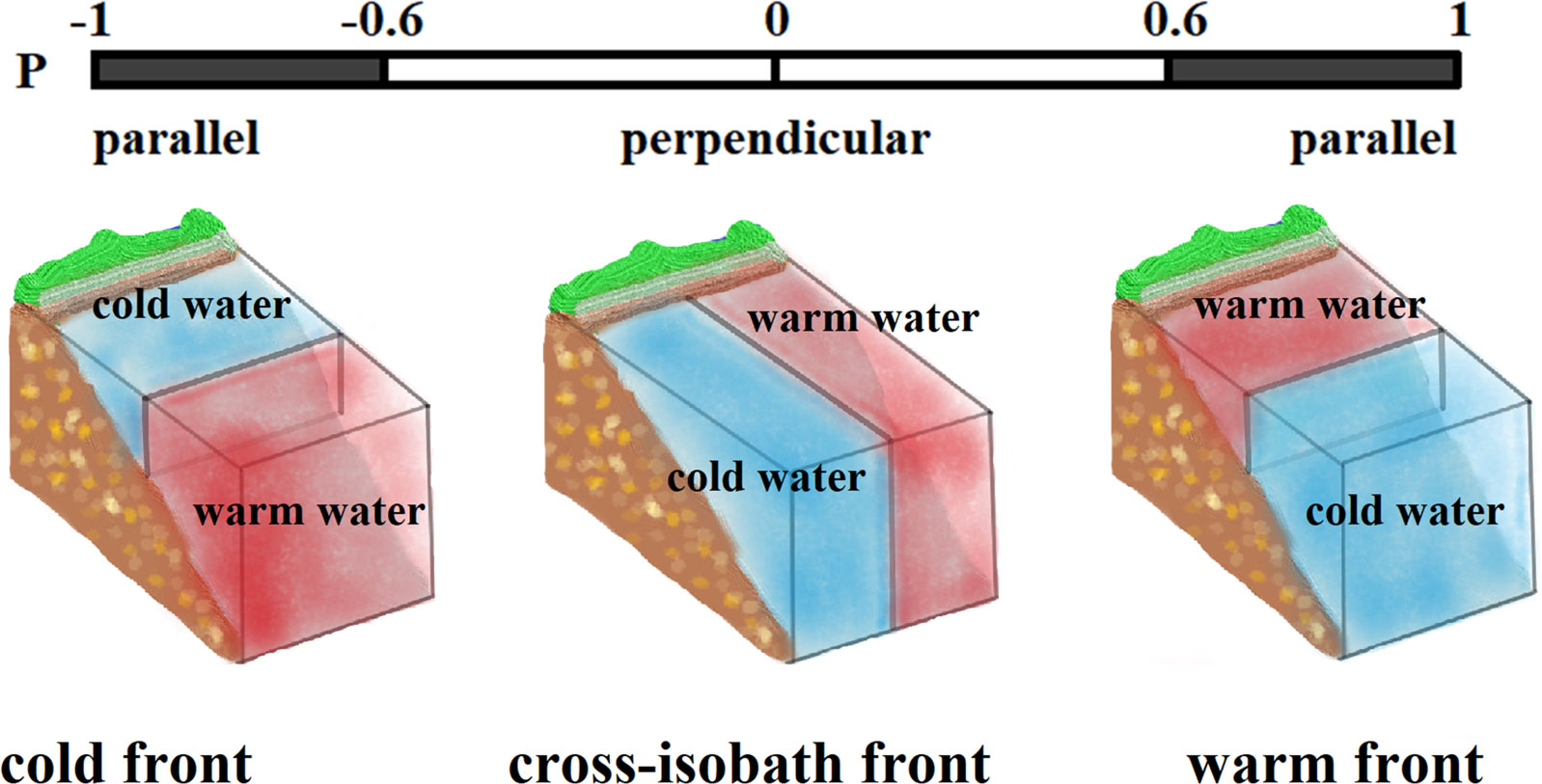
Figure 3 Seasonal SST averaged over 2002-2021 for (A) winter (January-March), (B) spring (April-June), (C) summer (July-September), and (D) autumn (October-December).The black lines are the 50-m and 200-m isobaths.
Seasonal variations of cold and warm fronts
Spatial variability
In order to determine the distribution of cold and warm fronts over the period of 20 years, we first calculate the P-value at frontal pixels for each image, and then composite all the images from each season. The seasonal variations in the occurrence of cold and warm fronts are shown in Figure 4. A strong distinctive cold (warm) front is one whose P-value is close to −1(1). Also, the seasonal FP (Figure 5), frontal gradient magnitude (Figure 6) and direction (Figure 7) are presented separately. In the following description, the frontal probabilities are categorized into three regimes: low (5%−10%), moderate (10%−20%), and high (> 20%).
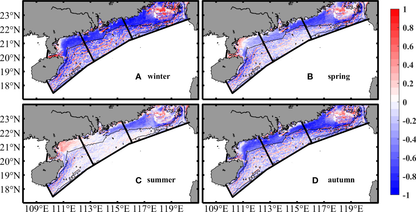
Figure 4 Seasonal distribution of cold and warm fronts averaged over 2002-2021 for (A) winter(January-March), (B) spring(April-June), (C) summer (July-September), and (D) autumn (October-December). Blue (red) represent cold(warm) fronts.The black lines are the 50-m and 200-m isobaths.
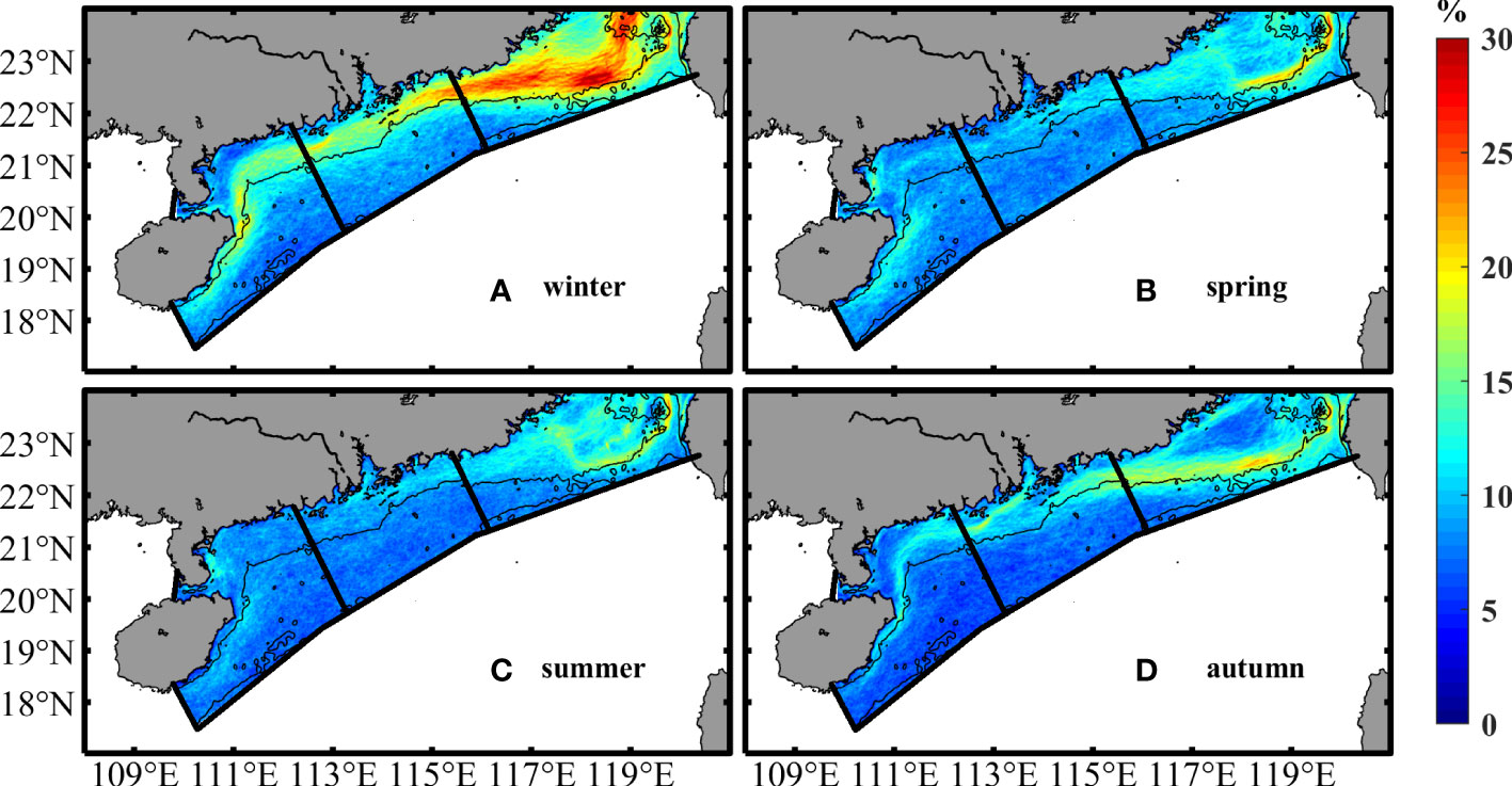
Figure 5 Seasonal frontal probability averaged over 2002-2021 for (A) winter (January-March), (B) spring (April-June), (C) summer (July-September), and (D) autumn (October-December).The black lines are the 50-m and 200-m isobaths.
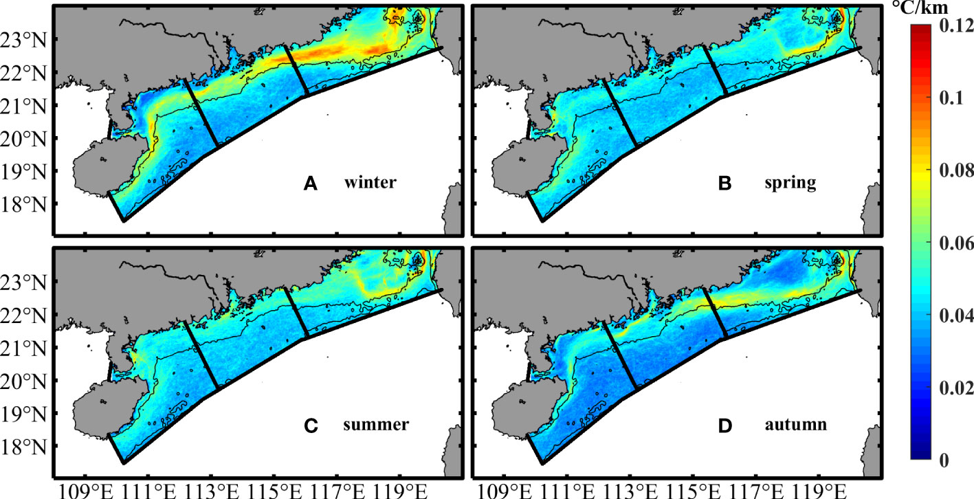
Figure 6 Mean SST gradient magnitude at frontal pixels averaged over 2002−2021 for (A) winter (January−March), (B) spring (April−June), (C) summer (July−September), and (D) autumn (October−December).The black lines are the 50-m and 200-m isobaths.
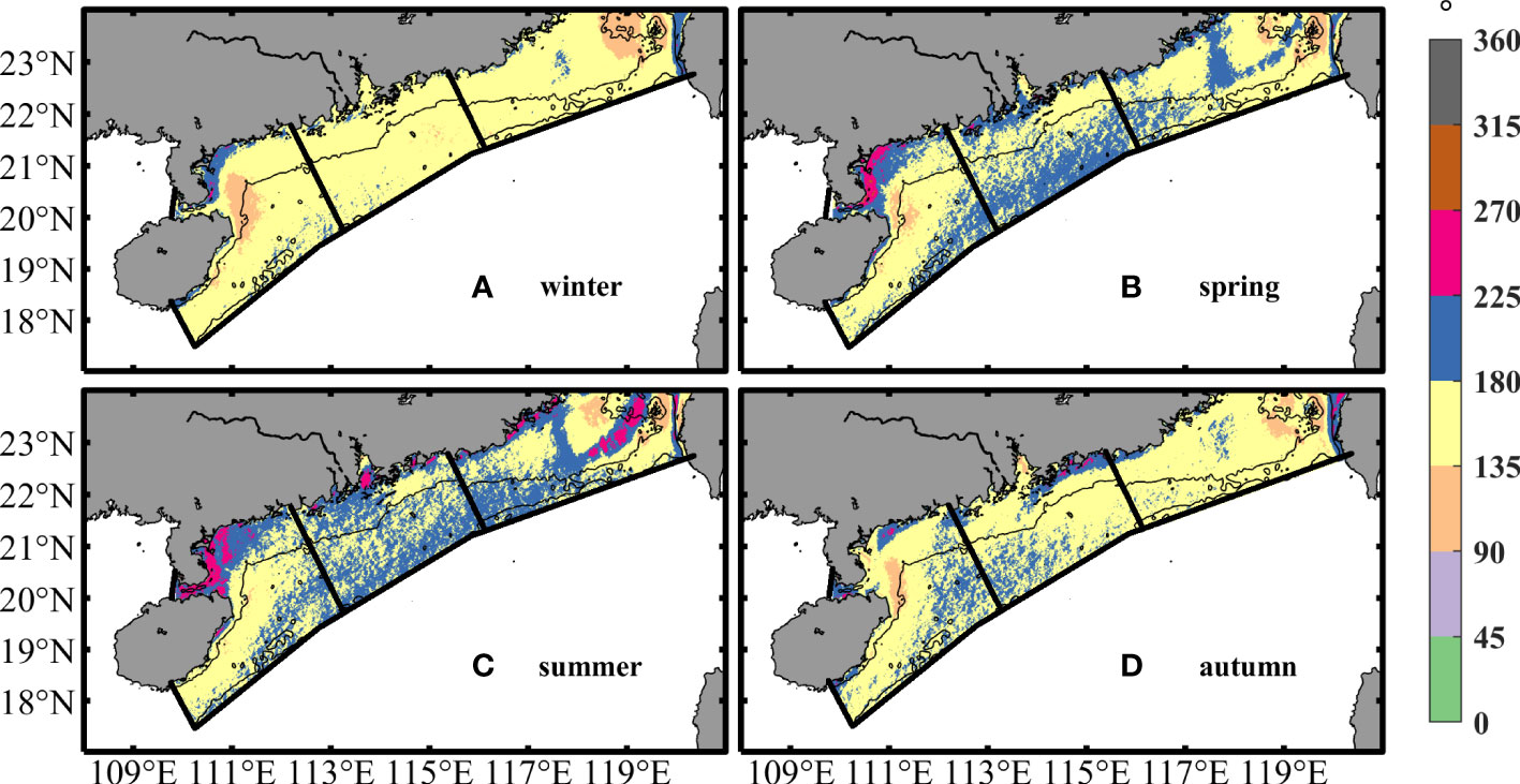
Figure 7 Mean SST gradient direction at frontal pixels averaged over 2002−2021 for (A) winter(January−March), (B) spring(April−June), (C) summer (July−September), and (D) autumn(October−December).The black lines are the 50-m and 200-m isobaths.
Winter
In subregion 1, large-scale and pronounced cold fronts are observed in a broad band off the Guangdong coast, whereas warm fronts mainly appear around the Taiwan Shoal (Figure 4A). The crescent-shape highest probability zone (20−30%) is located on the onshore side of 50-m depth (Figure 5A). Over the continental shelf, the frontal gradient magnitudes on average range from 0.06 to 0.1°C/km (Figure 6A). The frontal gradient direction suggests the existence of a nearshore cold water (Figure 7A), consistent with the intrusion of cold water flowing southward along the Guangdong coast.
In subregion 2, there is a broad band of cold fronts within the 50-m isobath, with dispersed warm fronts near the PRE. These fronts have a moderate to high probability (Figure 5A), with offshore gradients (Figure 7A), closely associated with the mixing of the cool river discharge with the warm nearshore water. Finer-scale cold and warm fronts are sporadically scattered throughout the wide continental shelf between 50- and 200-m isobaths (Figure 4A), with a low probability (5−10%) and gradient magnitude (0.03−0.05°C/km).
In subregion 3, most of the nearshore areas are occupied by a right-angle-shaped cold front band, while a small area of warm fronts can be found off the Zhanjiang coast (Figure 4A). These fronts have a moderate probability, with their peak approximately along the 50m isobath (Figure 5A). The frontal gradient directions are 180°−225° off the coast of Zhanjiang, but 90°−135° to the east of Hainan (Figure 7A).
Spring
In subregion 1, while there are no noticeable spatial changes in the warm- and cold fronts pattern, the frontal probability has significantly decreased (Figure 5B). Around the Taiwan Shoal, a small band on the onshore side of the 50-m isobath has the highest frontal probabilities (about 20%). The gradient directions reveal that the fronts in the center of the shoal are roughly oriented northwest, while the surrounding cold fronts are directed northeast (Figure 7B).
In subregion 2, cold fronts continue to diminish on the shallow side of 50-m isobath around the PRE (Figure 4B). However, the fronts on the east side of the PRE are much larger than those on the west side in the terms of P-value, frontal probability, and gradient (Figures 5B, 6B). In the area between 50- and 200-m isobaths, the finer-scale warm- and cold fronts weaken, accompanied by a decrease in frontal probability (Figure 4B). These fronts steer northeast, probably an early signal of the SCS Warm Current (Figure 7B).
In subregion 3, cold fronts are primarily located off the western Guangdong and the coast of Hainan, while warm fronts appear around the Zhanjiang coast and the Qiongzhou Strait (Figure 4B). Each of these fronts has a low to moderate probability (Figure 5B). The gradient directions indicate that these fronts are created by southward warm water and cool nearshore water (Figure 7B).
Summer
In subregion 1, the spatial pattern of warm- and cold fronts is relatively stable, but the P-value and frontal probability are further decreased (Figures 4C, 5C). In contrast to spring, the frontal gradient does somewhat rise (Figure 6C). The gradient directions indicate that there is cold water close to the eastern Guangdong and Taiwan coasts (Figure 7C), due to the upwelling occurrence induced by the summer monsoon. The upwelling could create stronger fronts in summer than in spring, while surface heating may play a secondary role.
In subregion 2, warm fronts appear in the western portion of PRE within 50 m isobath, whereas cold fronts appear in the eastern portion (Figure 4C). The probability of both fronts is low probabilities (Figure 5C), smaller than in the spring. On the west side of PRE, the fronts have even more pronounced decline. The frontal gradients are largest near the PRE, and exhibit little variation, revealing a complex system of both river and offshore currents (Figure 6C).
In subregion 3, over the continental shelf, cold fronts mainly exist on the continental shelf to the east of Hainan. Weak warm fronts dominate in the nearshore area off the western Guangdong coast (Figure 4C), where the probability is further decreased (Figure 5C) with no insignificant variation in the frontal gradients (Figure 6C). The gradient directions suggest that the cold fronts are closely related to the local coastal upwelling (Figure 7C).
Autumn
In subregion 1, warm fronts appear around the Taiwan Shoal, and a vast range of strong cold front band reappears off the coast of eastern Guangdong (Figure 4D). These fronts have the highest probability observed in a relatively limited zone along the 50-m isobath (Figure 5D). The pattern of the frontal gradients is well consistent with the probability (Figure 6D). The frontal gradient directions indicate that the shoal is dominated by southward-flowing cool water (Figure 7D).
In subregion 2, the band of strong cold front reappears within the 50 m depth (Figure 4D). A zone of moderate probability surrounds the PRE and extends to the west side (Figure 5D). The formation of the cold fronts is closely associated with the relatively cool river discharge. Also, the activity of finer-scale warm- and cold fronts between 50- and 200- m isobaths gradually become stronger (Figure 4D).
In subregion 3, the cold fronts occupy a large portion of the coastal zone from the western Guangdong to Hainan Island, while warm fronts are essentially absent (Figure 4D). A narrow moderate probability band which originates from the PRE is generally located well inside the 50-m isobath. The frontal gradient directions are generally oriented to southward, indicating that the cold fronts may be the result of southwestward-flowing cold water from the Pearl River (Figure 7D).
Temporal variability
To quantitatively represent the temporal variability of the frontal properties, we first calculate, at each frontal pixel, the frontal temperature, SST gradient, cross-frontal temperature step, frontal proportion (i.e., the ratio of the number of warm or cold fronts to the number of total fronts), frontal probability, and water depth. These time series are subsequently averaged over all frontal pixels in the each subregion to obtain the corresponding mean time series for the entire 20 years (2002–2021).
Figure 8 shows the time evolution of the mean temperature (T), mean cross-frontal temperature step (ΔT), mean gradient (∇T), and cross-frontal length scale (L) for each of the three subregions. Generally, each frontal property has similar significant seasonal variability for all the subregions. The mean SST has a maximum in summer and a minimum in winter (Figures 8A–C). The mean cross-front temperature step and cross-frontal length scale tend to reach their peaks in January-February before gradually decreasing from spring to summer (Figures 8D–I). The mean temperature step varies from 0.2 to 0.4°C (Figures 8D–F), and the cross-frontal length scale ranges from 6 to 9 km (Figures 8G–I), with large values occurring in January-December. The frontal gradient ranges from 0.02 to 0.07°C/km. It peaks in January and then declines through September, with a slow increase in July (Figures 8J–L).
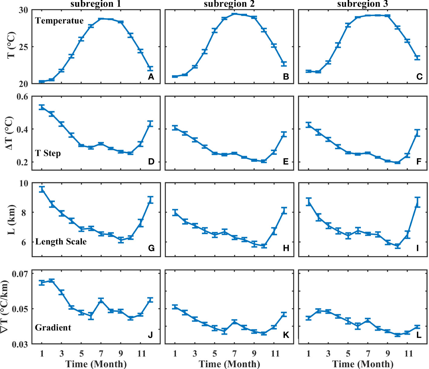
Figure 8 Mean monthly time series of frontal temperature (A–C), cross-frontal temperature step (D–F), cross-frontal length scale (G–I), cross-frontal temperature gradient (J–L) for the three subregions averaged over 2002-2021. The error bars denote the 95% confidence intervals.
Figure 9 shows the time evolution of the mean frontal proportion, mean frontal probability, mean frontal gradient and mean frontal water depth of the cold- and warm fronts for each of the three subregions. In the three subregions, the cold and warm frontal proportion varies in the opposite directions (Figures 9A–C). The mean proportion of the cold fronts is much higher compared with the warm fronts. Up to 70% of the cold fronts occur in winter, and then steadily drop to the lowest level in summer. In contrast, the proportion of the warm fronts reaches a maximum in summer and a minimum in winter. The mean FP of the cold fronts fluctuates roughly with its proportion, while the mean FP of the warm fronts shows less significant variability (Figures 9D–F). The mean frontal probability ranges from 2 to 3% for the warm fronts, and from 3 to 9% for the cold fronts, indicating that the cold fronts are primarily responsible for changes in the ratio of warm to cold fronts. The mean frontal gradient generally has similar variability for the cold and warm fronts. It ranges from 0.03 to 0.07°C/km (Figures 9G–I). For the mean frontal water depth, large differences between the cold and warm fronts are very apparent in the three subregions (Figures 9J–L). The cold fronts in the subregions 2 and 3 obviously move offshore in summer and onshore in winter, in opposite to the warm fronts, whereas there is little variation in the warm and cold front positions in the subregion 1.
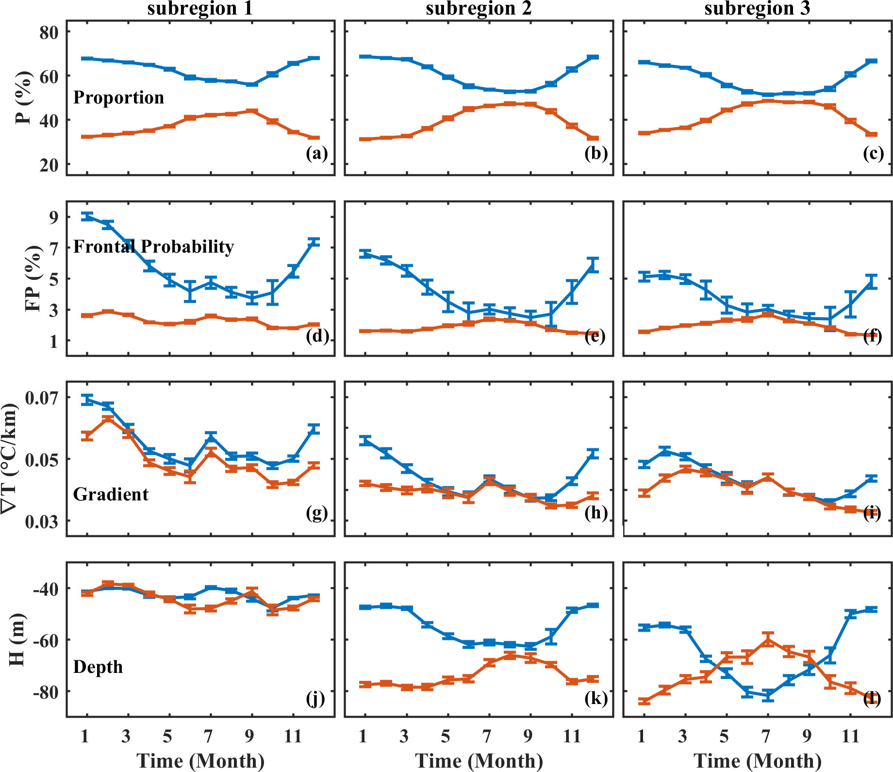
Figure 9 Mean monthly time series of cold and warm fronts in proportion (A–C), frontal probability (D–F), cross-frontal gradient (G–I), and depth (J–L) at fronts for the three subregions averaged over 2002−2021. Blue (red) lines correspond to the cold (warm) fronts. The error bars denote the 95% confidence intervals.
To further understand the spatiotemporal variability of SST fronts, the empirical orthogonal function (EOF) analysis is performed for 20 years of monthly FP data including both cold and warm fronts. In this study, we only show the first EOF mode which could account for 11.27% of the total variance, since the second mode accounts for less than 4% of the variance. The first EOF mode and its time series amplitude are shown in Figure 10. Around the Taiwan Shoal, off the Guangdong coast, and to the east of Hainan, a significant EOF magnitudes are very apparent. The corresponding monthly mean time series also confirm the significant seasonal variability (Figure 10B), with peaks in January and troughs in September.
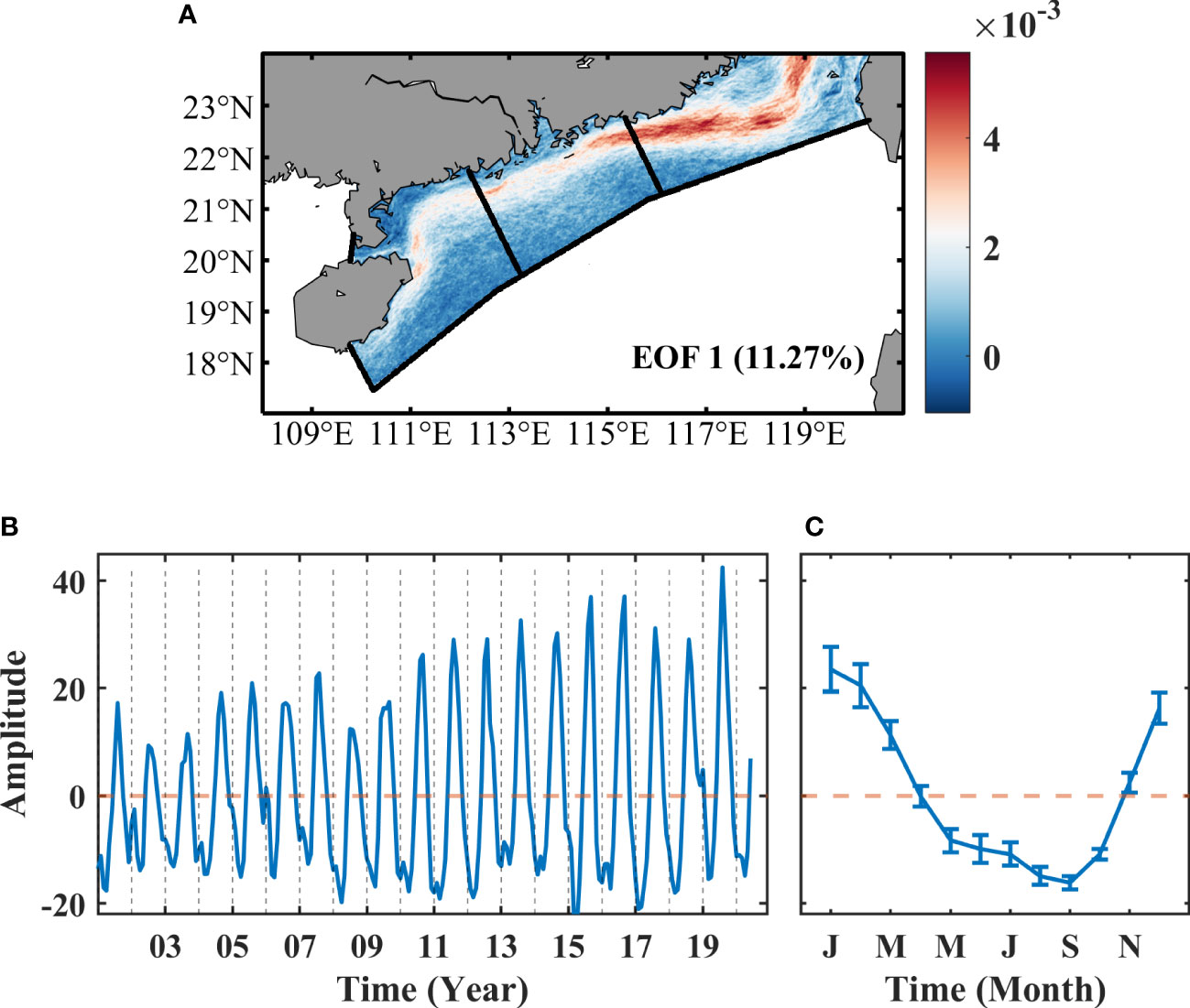
Figure 10 The first EOF mode (A), its corresponding time series for FP (B), and the mean monthly amplitudes averaged over the 20-yr period (C).
Discussion and conclusions
In this study, the cold- and warm-thermal fronts, and their seasonal variability over the NSCS shelf are investigated based on 20 years of high-resolution GHRSST images. Over the shallow continental shelf (< 50 m), a long and wide band of strong cold fronts is most frequently observed in winter, with weaker, less frontal activity present during other seasons. The persistence of the cold fronts may result from the advection of relatively cool water from the high latitudes by southwestward coastal cold current (i.e., Guangdong Coastal Current, GCC). The GCC offshore of the eastern Guangdong coast flows southwestward in winter and northeastward in summer (Guan and Chen, 1964; Fang et al., 1998), while offshore of the western Guangdong coast the GCC flows westward during both winter and summer (Ying, 1999; Bao et al., 2005; Xie et al., 2012). Also, a warm current exists south of the GCC. This current (i.e., South China Sea Warm Current) originates from east of Hainan Island and flows northeastward along the NSCS shelf against the northeasterly winds in winter (Guan, 1978; Fang et al., 1995; Guan and Fang, 2006), thus increasing the temperature contrast between coastal water and outer shelf water and leading to strengthen the cold fronts.
The summer fronts have showed that the warm fronts occur predominantly off the western Guangdong coast and the cold fronts are mainly observed off the eastern Guangdong coast and the eastern Hainan Island, despite relatively low probability and gradient magnitude. These fronts are possibly a response to the summer wind stress and the GCC. For the prevailing southwest summer monsoon, an alongshore component can induce offshore Ekman transport, thereby triggering coastal upwelling along the coast of the eastern Guangdong and the eastern Hainan Island (Jing et al., 2016; Shu et al., 2018). The upwelling would bring relatively cold bottom water to the surface, separating cool vertically mixed water in shallow areas from warm stratified offshore water in deep areas to form cold fronts. On the other hand, over the western inner shelf off the Guangdong coast, direct measurements suggested that the western inner shelf of Guangdong is mainly occupied by the warm GCC which primarily flows westward along the coast for summer monsoon (Yang et al., 2003; Chen et al., 2006). A relatively cold tongue appears south of the GCC and stretches northeastward from northeast of Hainan Island approximately along the 50-m isobath (Figure 2C). The combined effect of the GCC and the relatively cool northeastward-flowing water is presumably responsible for the formation of the warm fronts.
There is a very distinct separation between the nearshore fronts on the inner shelf and the offshore fronts in the vicinity of the 50-m isobath, suggesting that a different mechanism induces the formation of the latter. Due to the most rapid changes of the bottom slope, the 50-m isobath seems to be the preferred location for frontogenesis. Garwood et al. (1981) suggested that the SST front formation could result from surface cooling over the midshelf where the shelf depth is shallower than the depth of wind-induced mixing. A similar effect could occur over the NSCS shelf. During both winter and autumn, the inner shelf of the NSCS is vertically well mixed because of the surface cooling and severe northeast monsoon, the depths of mixed layer are about 40-60 m (Wu and Chen, 2013). The uniform surface cooling can lead to a stronger offshore temperature gradient roughly along the 50-m isobath. Simultaneously, the winds can also induce a vigorous shoreward transport of warm surface water from the outer shelf (Jing et al., 2016). The joint effect of onshore surface Ekman transport of warm water and surface cooling of cold air is responsible for the midshelf frontogenesis, which is consistent with the findings of Oey (1986) in the South Atlantic Bight.
A striking aspect of the fronts to observe for the first time is that the finer-scale warm- and cold fronts discretely occur over the outer shelf (>50 m), with the aid of the high spatial resolution satellite images. These frontal activities are most observed in winter and then gradually decrease to become minimum in summer, despite relatively weak intensity and low probability of frontal activities. The fronts are possibly due to the ubiquitous submesoscale processes in the SCS (Lin et al., 2020; Ni et al., 2021; Qiu et al., 2022). Lin et al. (2020) characterized the SCS mesoscale and submesoscale features based on a submesoscale-permitting numerical simulation (MITgcm llc4320). They found that the submesoscale features in the NSCS is very rich and undergo significant seasonal variations. The submesoscale activities over the outer NSCS shelf are vigorous in winter but slightly quiescent in summer. Their findings are well consistent with our satellite observations.
Satellite remote sensing could only provide the surface signature of cold- and warm fronts. To fully understand their formation mechanisms, multiple vertical profile hydrographic data with high-enough spatiotemporal resolution, is still needed for analysis in a future study. In addition, previous studies have emphasized the important role of the cold- and warm fronts in the biogeochemical processes (e.g., Chang et al., 2008). The ecological effect of the cold- and warm fronts and the corresponding spatial and temporal variability in the SCS will be quantitatively analyzed in our following paper.
Data availability statement
Publicly available datasets were analyzed in this study. This data can be found here: https://podaac.jpl.nasa.gov/dataset.
Author contributions
ZH: Conceptualization, Methodology, Writing– review and editing, Funding acquisition. JC: Formal analysis, Data curation, Writing – original draft and Writing – review and editing. All authors contributed to the article and approved the submitted version.
Funding
This work is jointly funded by the National Natural Science Foundation of China (No. 41706205; 42176029), and the Innovation Group Project of Southern Marine Science and Engineering Guangdong Laboratory (Zhuhai) (No. 311020004).
Acknowledgments
The authors would like to thank the Physical Oceanography Distributed Active Archive Center (PO.DAAC) of the National Aeronautics and Space Administration (NASA) for sharing the satellite dataset (https://podaac.jpl.nasa.gov/dataset). We would like to acknowledge Shimada for algorithm support and an three reviewers whose comments have helped to improve the presentation of this paper.
Conflict of interest
The authors declare that the research was conducted in the absence of any commercial or financial relationships that could be construed as a potential conflict of interest.
The reviewer XZ declared a shared affiliation with the author ZH to the handling editor at the time of review.
Publisher’s note
All claims expressed in this article are solely those of the authors and do not necessarily represent those of their affiliated organizations, or those of the publisher, the editors and the reviewers. Any product that may be evaluated in this article, or claim that may be made by its manufacturer, is not guaranteed or endorsed by the publisher.
References
Bao X., Hou Y., Chen C., Chen F., Shi M. (2005). Analysis of characteristics and mechanism of current system on the west coast of guangdong of China in summer. Acta Oceanologica Sin. 24, 1–9.
Chang Y., Cornillon P. (2015). A comparison of satellite-derived sea surface temperature fronts using two edge detection algorithms. Deep-Sea Res. Part Ii-Topical Stud. Oceanogr. 119, 40–47. doi: 10.1016/j.dsr2.2013.12.001
Chang Y., Lee M. A., Shimada T., Sakaida F., Kawamura H., Chan J. W., et al. (2008). Wintertime high‐resolution features of sea surface temperature and chlorophyll‐a fields associated with oceanic fronts in the southern East China Sea. International Journal of Remote Sensing 29(21), 6249–6261.
Chen J. (1983). Some explanation of sea surface temperature distribution in northern south China Sea in winter. Acta Oceanologica Sin. 5 (3), 391–395+397-398.
Chen D., Chen B., Jinhui Y. A. N., Huifen X. U. (2006). The seasonal variation characteristics of residual currents in the qiongzhou strait. Trans. Oceanol. Limnol. 2), 12–17. doi: 10.3969/j.issn.1003-6482.2006.02.003
Chen G. X., Gan J. P., Xie Q., Chu X. Q., Wang D. X., Hou Y. J. (2012). Eddy heat and salt transports in the south China Sea and their seasonal modulations. J. Geophysical Research-Oceans 117, C05021. doi: 10.1029/2011jc007724
Chu P. C., Wang G. H. (2003). Seasonal variability of thermohaline front in the central south China Sea. J. Oceanogr. 59 (1), 65–78. doi: 10.1023/A:1022868407012
Fang G., Fang W., Fang Y., Wang K. (1998). A survey of studies on the south China Sea upper ocean circulation. Acta Oceanographica Taiwanica 37, 1–16.
Fang G. H., Zhao J. P., Bole J., Mathisen J. P., Schjolberg P., Pan H. (1995). Circulation, internal tides and solitons at the shelf break of the northern south China Sea–An analysis of measured currents. p. 50–51. In Marine Science Conference in Taiwan Adjacent Seas—Program and Abstracts, Taipei, Taiwan.
Fedorov K. N. (1986). The physical nature and structure of oceanic fronts (New York, NY: Springer-Verlag), 10010. Medium: X; Size: Pages: 333 2008-2002-2007. doi: 10.1029/LN019
Fournier R. O. (1978). Biological aspects of the Nova scotian shelfbreak fronts. Oceanic Fronts Coast. Processes Bowman M. J., Esaias W. E., (New York: Springer-Verlag) 69–77.
Garwood R. W. Jr., Fett R. W., Rabe K. M., Brandli H. W. (1981). Ocean frontal formation due to shallow water cooling effects as observed by satellite and simulated by a numerical method. J. Geophysical Res. 86 (C11), 11000–11012. doi: 10.1029/JC086iC11p11000
Guan B. (1978). The warm current in the south China Sea–a current flowing against the wind in winter in the open sea off guangdong province. Oceanol. Limnol. Sin. 9, 117–127.
Guan B., Chen S. (1964). The current systems in the near-Sea area of China seas (in Chinese). Tech. Rep. pp. 1–85.
Guan B., Fang G. (2006). Winter counter-wind currents off the southeastern China coast: A review. J. Oceanogr. 62 (1), 1–24. doi: 10.1007/s10872-006-0028-8
Guo L., Xiu P., Chai F., Xue H. J., Wang D. X., Sun J. (2017). Enhanced chlorophyll concentrations induced by kuroshio intrusion fronts in the northern south China Sea. Geophysical Res. Lett. 44 (22), 11565–11572. doi: 10.1002/2017gl075336
Hu Z., Pan D., He X., Bai Y. (2016). Diurnal variability of turbidity fronts observed by geostationary satellite ocean color remote sensing. Remote Sens. 8 (2), 147. doi: 10.3390/rs8020147
Hu Z., Xie G., Zhao J., Lei Y., Xie J., Pang W. (2021). Mapping diurnal variability of the wintertime pearl river plume front from himawari-8 geostationary satellite observations. Water 14 (1), 43. doi: 10.3390/w14010043
Jing Z., Qi Y., Fox-Kemper B., Du Y., Lian S. (2016). Seasonal thermal fronts on the northern south China Sea shelf: Satellite measurements and three repeated field surveys. J. Geophysical Research: Oceans 121 (3), 1914–1930. doi: 10.1002/2015jc011222
Legeckis R. (1978). A survey of worldwide sea surface temperature fronts detected by environmental satellites. J. Geophysical Research: Oceans 83 (C9), 4501–4522. doi: 10.1029/JC083iC09p04501
Lin H., Liu Z., Hu J., Menemenlis D., Huang Y. (2020). Characterizing meso- to submesoscale features in the south China Sea. Prog. Oceanogr. 188, 102420. doi: 10.1016/j.pocean.2020.102420
Liu K. K., Chao S. Y., Shaw P. T., Gong G. C., Chen C. C., Tang T. Y. (2002). Monsoon-forced chlorophyll distribution and primary production in the south China Sea: Observations and a numerical study. Deep-Sea Res. Part I-Oceanographic Res. Papers 49 (8), 1387–1412. doi: 10.1016/S0967-0637(02)00035-3
Ni Q., Zhai X., Wilson C., Chen C., Chen D. (2021). Submesoscale eddies in the south China Sea. Geophysical Res. Lett. 48 (6), e2020GL091555. doi: 10.1029/2020gl091555
Oey L.-Y. (1986). The formation and maintenance of density fronts on the U.S. southeastern continental shelf during winter. J. Phys. Oceanogr. 16 (6), 1121–1135. doi: 10.1175/1520-0485(1986)016<1121:Tfamod>2.0.Co;2
Qiu C., Yang Z., Wang D., Feng M., Su J. (2022). The enhancement of submesoscale ageostrophic motion on the mesoscale eddies in the south China Sea. J. Geophysical Research-Oceans 127 (9), e2022JC018736. doi: 10.1029/2022jc018736
Qu T. D., Du Y., Gan J. P., Wang D. X. (2007). Mean seasonal cycle of isothermal depth in the south China Sea. J. Geophysical Research-Oceans 112 (C2), C02020. doi: 10.1029/2006jc003583
Ren S., Wang H., Liu N. (2015). Review of ocean front in Chinese marginal seas and frontal forecasting. Advance Earth Sci. 30 (5), 552–563. doi: 10.11867/j.issn.1001-8166.2015.05.0552
Shimada T., Sakaida F., Kawamura H., Okumura T. (2005). Application of an edge detection method to satellite images for distinguishing sea surface temperature fronts near the Japanese coast. Remote Sens. Environ. 98 (1), 21–34. doi: 10.1016/j.rse.2005.05.018
Shu Y., Wang Q., Zu T. (2018). Progress on shelf and slope circulation in the northern south China Sea. Sci. China-Earth Sci. 61 (5), 560–571. doi: 10.1007/s11430-017-9152-y
Ullman D. S., Cornillon P. C. (1999). Satellite-derived sea surface temperature fronts on the continental shelf off the northeast US coast. J. Geophysical Research-Oceans 104 (C10), 23459–23478. doi: 10.1029/1999jc900133
Ullman D. S., Cornillon P. C. (2001). Continental shelf surface thermal fronts in winter off the northeast US coast. Continental Shelf Res. 21 (11-12), 1139–1156. doi: 10.1016/S0278-4343(00)00107-2
Wang D., Liu Y., Qi Y., Shi P. (2001). Seasonal variability of thermal fronts in the northern south China Sea from satellite data. Geophysical Res. Lett. 28 (20), 3963–3966. doi: 10.1029/2001gl013306
Wang G. H., Li J. X., Wang C. Z., Yan Y. W. (2012). Interactions among the winter monsoon, ocean eddy and ocean thermal front in the south China Sea. J. Geophysical Research-Oceans 117, C08002. doi: 10.1029/2012jc008007
Wang Y., Yu Y., Zhang Y., Zhang H. R., Chai F. (2020). Distribution and variability of sea surface temperature fronts in the south China sea. Estuarine Coast. Shelf Sci. 240, 106793. doi: 10.1016/j.ecss.2020.106793
Wu Y., Chen G. (2013). Seasonal and inter-annual variations of the mixed layer depth in the south China Sea. Mar. Forecasts. 30, 9–17. doi: 10.11737/j.issn.1003-0239.2013.03.002
Xie L., Cao R., Shang Q. (2012). Progress of study on coastal circulation near the shore of Western guangdong. Guangdong Ocean Univ 32, 94–98. doi: 10.3969/j.issn.1673-9159.2012.04.019
Yang S., Bao X., Chen C., Chen F. (2003). Analysis on characteristics and mechanism of current system in west coast of guangdong province in the summer. Acta Oceanologica Sin. 25 (6), 1–8. doi: 10.3321/j.issn:0253-4193.2003.06.001
Yao J. L., Belkin I., Chen J., Wang D. X. (2012). Thermal fronts of the southern south China Sea from satellite and in situ data. Int. J. Remote Sens. 33 (23), 7458–7468. doi: 10.1080/01431161.2012.685985
Ying B. (1999). On the coast current and its deposit along Western coast in guangdong. Acta Scientiarum Naturalium Universitis Sunyatseni 38, 85–89.
Keywords: cold fronts, warm fronts, spatial patterns, seasonal variability, the northern South China Sea
Citation: Chen J and Hu Z (2023) Seasonal variability in spatial patterns of sea surface cold- and warm fronts over the continental shelf of the northern South China Sea. Front. Mar. Sci. 9:1100772. doi: 10.3389/fmars.2022.1100772
Received: 17 November 2022; Accepted: 27 December 2022;
Published: 18 January 2023.
Edited by:
Xiaoteng Shen, Hohai University, ChinaReviewed by:
Wenjin Sun, Nanjing University of Information Science and Technology, ChinaQiyan Ji, Zhejiang Ocean University, China
Yu Liu, Zhejiang Ocean University, China
Copyright © 2023 Chen and Hu. This is an open-access article distributed under the terms of the Creative Commons Attribution License (CC BY). The use, distribution or reproduction in other forums is permitted, provided the original author(s) and the copyright owner(s) are credited and that the original publication in this journal is cited, in accordance with accepted academic practice. No use, distribution or reproduction is permitted which does not comply with these terms.
*Correspondence: Zifeng Hu, aHV6aWZlbmdAbWFpbC5zeXN1LmVkdS5jbg==