A new non-invasive tagging method for leopard coral grouper (Plectropomus leopardus) using deep convolutional neural networks with PDE-based image decomposition

External tagging methods can aid in the research of leopard coral grouper (Plectropomus leopardus) in terms of its spatio-temporal behavior at population and individual scales. However, due to the strong exclusion ability and the damage to the body wall of P. leopardus, the retention rate of traditional invasive tagging methods is low. To develop a non-invasive identification method for P. leopardus, we adopted a multiscale image processing method based on matched filters with Gaussian kernels and partial differential equation (PDE) multiscale hierarchical decomposition with the deep convolutional neural network (CNN) models VGG19 and ResNet50 to extract shape and texture image features of individuals. Then based on image features, we used three classifiers Random forest (RF), support vector machine (SVM), and multilayer perceptron (MLP)) for individual recognition on sequential images of P. leopardus captured for 50 days. The PDE, ResNet50 and MLP combination obtained a maximum accuracy of 0.985 ± 0.045 on the test set. For individual temporal tracking recognition, feature extraction and model training were performed using images taken in 1-20 days. The classifier could achieve an accuracy of 0.960 ± 0.049 on the test set consisting of images collected in the periods of 20-50 days. The results show that CNNs with the PDE decomposition can effectively and accurately identify P. leopardus.

1 Introduction

P. leopardus represents one of the most economically significant chordate and is mainly distributed in the Western Pacific Ocean along the coasts of China, Vietnam, and Thailand (Yang et al., 2020). P. leopardus has a high economic value in the international market due to its high nutritional profile and plays a vital role in marine ecosystems (Xia et al., 2020). However, the P. leopardus industry has encountered many challenges in recent years, including devastating diseases and environmental stresses, which caused a large amount of economic loss and hampered the healthy and sustainable development of the P. leopardus industry (Rimmer and Glamuzina, 2019). Therefore, it is urgent to advance the scientific culture of P. leopardus and to select and breed new species with superior characteristics. Designing effective external tagging methods for long-term and stable tracking identification of P. leopardus is not only essential for successful breeding but also a concern for ecologists conducting population dynamics studies (Williams et al., 2002; Zhuang et al., 2013), as well as revealing the ecological significance of fish endotherms (Watanabe et al., 2015), and studying the life history of fish such as foraging, migration and reproduction (Quinn et al., 1989; Ogura and Ishida, 1995; Yano et al., 1996; Hinch et al., 2002; Welch et al., 2004; Sulak et al., 2009; Døving et al., 2011).

Traditionally, individual recognition has been accomplished by capturing animals and placing visible and unique marks on them. The traditional marking methods include implanting acoustic markers inside the abdominal cavity of fish (Shi et al., 2022), and then using the positioning system to track the acoustic markers. The individual unique electric field generated by electric fish discharges was used for recording and tracking (Raab et al., 2022). Due to the strong exclusion ability and the damage to the body of P. leopardus, the retention rate of traditional invasive tagging methods is low (Bolger et al., 2012). Besides, the infection rate and mortality rate of implanted marker fish are relatively high (Shi et al., 2022), and the marker will also affect the original normal life of fishes in the water, and with the extensive use of individual markers, it is also a hazard to the environment (Šmejkal et al., 2020), while individual electric field tracking is only applicable to fish that can generate electricity. This makes it difficult for breeders to manage good individuals, which is not conducive to the implementation of accurate breeding by tracking the growth of individuals. Recently, molecular genetic markers such as RFLP (restriction fragment length polymorphism), RAPD (random amplified polymorphism DNA), SSR (simple sequence repeat), and SNP (single nucleotide polymorphism) have also been widely used to study the population and individual recognition (Reed et al., 1997; Wang, 2016). However, these methods are not suitable for a larger population because of inconsistency, inconvenience, and higher cost, among others. Currently, photographic mark-recapture has gained popularity because of the advances in digital photography and image processing software. The abundance of species with variable natural marking patterns makes this an attractive method for many researchers. The image mark method has been employed particularly in the studies of populations of marine mammals and mammalian terrestrial predators (Karanth and Nichols, 1998; Forcada and Aguilar, 2000; Langtimm et al., 2004; Fearnbach et al., 2012). Some image processing methods have been used to extract, store, and compare pattern information from digital images (Bolger et al., 2012). With the development of computer vision, deep learning (DL) methods, such as convolutional neural networks (CNNs) are emerging as possibly powerful tools for individual recognition and long-term tracking (He et al., 2016; Redmon et al., 2016). Numerous broad models of convolutional neural networks, such as AlexNet, Inception, VGG19, ResNet50, etc., have been presented (Kamilaris and Prenafeta-Boldú, 2018). These models are trained using public datasets (e.g., CIFAR-10, ImageNet datasets, etc.) and used to perform Multi-Category tasks for particular items. Considering the unique body shape and texture patterns of different P. leopardus individuals, it is a promising technical route to extract and identify the body surface features using CNN as an alternative method against traditional invasive tagging methods.

In this study, we used a novel multiscale image processing method based on matched filters with Gaussian kernels and partial differential equation (PDE) multiscale hierarchical decomposition (Wang et al., 2013) to segment the shape features of P. leopardus images. Two deep CNN models, VGG19 and ResNet50, were implemented to extract the texture features. Then based on the shape and texture features, three classifiers (Random forest (RF) (Kamilaris and Prenafeta-Boldú, 2018), support vector machine (SVM) (Cortes and Vapnik, 1995), and multilayer perceptron (MLP) (LeCun et al., 2015) were compared for individual recognition on sequential images of P. leopardus captured over the course of 50 days. Finally, we found that the combination of PDE and CNN methods could achieve the best accurate recognition of P. leopardus. This is the first time, to our knowledge, that image recognition analysis has been applied to the tracking of P. leopardus. Our results will provide a new vision for using non-invasive tagging of P. leopardus.

2 Materials and methods

2.1 Data acquisition

P. leopardus used in this study were obtained from Sanya, Hainan Province. 50 individuals were randomly selected from a breeding population of 10,000 P. leopardus, and reared under laboratory conditions. The numbered clapboards were added to the rearing pool to facilitate individual identification. In the 50 days from September 3, 2022, to October 23 2022, each individual was taken out from the rearing pool daily and placed on a smooth white foam plastic plate. The P. leopardus were anesthetized by immersion in seawater which containing MS222 (tricaine methanesulfonate) with a concentration of 100 mg/L and kept in the solution for 3 min after loss of body posture (Savson et al., 2022). After its body was fully stretched, photos were taken directly for each individual using a mobile device. Then they were placed back in the pond immediately. At the end of the experiment, 50 images were taken for each individual. So, we obtained a total of 2500 images for all individuals.

2.2 Image feature extraction

2.2.1 PDE-based feature extraction

We used a PDE-based multiscale decomposition method to extract the shape features of P. leopardus images. For the shape detection, we used matched filtering with Gaussian kernel (MFGK) ker(x,y; a,b)=−exp(−a⁻¹(x−b)²/2σ²) (Chaudhuri et al., 1989), and the computed MFGK response image was as follows:

$\begin{array}{ll}{\text{M}}_{\text{ker}}\left(\text{x},\text{y};\text{a},\text{b}\right)={\text{max}}_{\text{θ}}\left({\text{r}}_{\text{θ}}\left(\text{ker}\left(\text{x},\text{y};\text{a},\text{b}\right)\right)*\text{Img}\left(\text{x},\text{y}\right)\right)& (1)\end{array}$

where Img, (x, y), σ, ker, a, and b denoted an image, a two-dimensional pixel position, the standard deviation of image gray value in Gaussian convolution kernel, two-dimensional Gaussian functions, the dilation parameter (also known as scaling parameter), and the translation parameter, respectively. r_θ rotated the kernel function with an angle θ, and * represented the convolution operation in variables (x and y).

The normalized response image was defined as follows:

$$\text{f}=\left({\text{M}}_{\text{ker}}\left(\text{x},\text{y};\text{a},\text{b}\right)-\text{μ}\right)/\text{s}$$

where μ and s were the mean and standard deviation of the enhanced MFGK image M_ker(x,y;a,b) The multiscale hierarchical decomposition of an image f was defined as follows (Wang et al., 2013). Given an initial scale parameter λ₀ and the PDE-based total variation (TV) function (Rudin et al., 1992)

$$\text{J}\left(\text{f},\text{ λ}\right)=\text{λ}{\left|\left|{\text{ v}}_{\text{λ}}\right|\right|}_{\text{L}2}^2+{\left|\left|{\text{ u}}_{\text{λ}}\right|\right|}_{\text{BV}}^{}$$

where BV stood for the homogenous bounded total variation space equipped with the norm of total variation

$${\left|\left|.\right|\right|}_{\text{BV}}^{}={\left|\left|.\right|\right|}_{{\text{L}}^1}^{}=\underset{\text{Ω}}{\overset{}{\int }}\sqrt{{({\text{u}}_{\text{λ}})}_{\text{x}}^2+{({\text{u}}_{\text{λ}})}_{\text{y}}^2}$$

$$f=u_0+v_0, where \left[u_0,v_0\right]:=argmin{\mid }_{u+v=f} J\left(f,{\text{ λ}}_0\right)$$

$$v_k=u_{k+1}+v_{k+1}, k=0,1,\dots ,{\lambda }_k={\lambda }_0{2}^{k+1}$$

where [u_k+1,v_k+1:=argmin∣_u+v=vkJ(v_k,λ₀2^k+1) ].

Based on the above enhancement with MFGK and multiscale hierarchical decomposition, many line maps u_λ were generated at varying image resolutions, representing different levels of line details to avoid the possible failure of feature extraction caused by a single-scale segmentation. The initial scaling parameter was λ₀ = 0.01 in the multiscale hierarchical decomposition.

The binarization is performed as follows:

$$\text{out}\left(\text{x},\text{y}\right)=\{\begin{array}{c}1 \overline{\text{u}}\left(x,y\right) \le u\left(x,y\right)\\ 0 otherwise\end{array}$$

where out stands for the finally segmented binary mask of the P. leopardus image.

2.2.2 CNN-based feature extraction

With the development of deep learning algorithms, many general models of convolutional neural networks have been proposed, such as AlexNet, Inception, VGGNet, ResNet, etc. (Kamilaris and Prenafeta-Boldú, 2018). These models have been trained on large public datasets (e.g., CIFAR-10, ImageNet datasets, etc.) (Lecun et al., 1998) to achieve the goal of multiple-classification tasks for specific items. After training, the deep layers and convolutional kernels in these models can explore the visual characteristics of images. For other classification tasks, new characteristics can be extracted with the help of the pre-trained convolutional layers and used as input for many classifiers. This method of applying the “knowledge” gained from training on a specific dataset to a new domain is also known as migration learning (Yoshua, 2011). In this study, the VGG19 and ResNet50 of CNN models were used for image feature extraction. The weights of each convolutional layer of VGG19 or ResNet50 were frozen and fed into a new CNN. The output of the last pooling layer of the new CNN was then taken as the extracted image features. After feature extraction using VGG19 or ResNet50, a 4096-1D or 2048-1D vector of features was obtained, respectively.

LeNet-5 Convolutional Neural Network (Lecun et al., 1998), as a classic CNN, has only two convolution layers and a simple structure, which is suitable for preliminary evaluation of the complexity of the dataset. The structure of the model is as follows. Input layer: single input is a 224*224*3 RGB three-channel image without feature extraction; convolutional layer 1, containing 6 convolutional kernels with the size of 5*5 pixels using activation function ReLU; batch normalization layer 1; maximum pooling layer 1, with the pooling size of 2*2; convolutional layer 2, containing 16 convolutional kernels with the size of 5*5 pixels using activation function ReLU; batch normalization layer 2; Maximum pooling layer 2, with the pooling size of 2*2; fully connected layer 1, containing 120 neurons using activation function ReLU; batch normalization layer 3; fully connected layer 2, containing 84 neurons using activation function ReLU; batch normalization layer 4; output layer, outputting 20 classes using activation function softmax. The loss function is cross entropy and the optimizer is Adam. When training on the raw dataset, batch_size is 30 and epoch is 50.

VGG is a type of CNN model developed by the Oxford Robotics Institute (Simonyan and Zisserman, 2015). VGG19 uses an architecture of very small (3x3) convolution filters and pushes the depth to 19 weight layers. There are five building blocks in VGG19, consisting of 16 convolutional layers and 3 fully connected layers. The first and second building blocks have two convolutional layers and one pooling layer, respectively, and four convolutional layers and one pooling layer exist in the third and fourth building blocks. The last building block contains four convolutional layers.

The architecture of the residual network consists of 50 layers named ResNet50 (He et al., 2016). There is an extra identity in ResNet50 where the ResNet model predicts the delta needed in the final prediction from one layer to the next. ResNet50 provides alternate paths to allow gradient flow which helps to solve the problem of gradient disappearance. The ResNet model uses identity mapping to bypass the weight layer of the CNN when the current layer is not required. This model solves the overfitting problem of the training set with the presence of 50 layers in the feature extraction of ResNet50 (Stateczny et al., 2022).

In this study, the PDE-based multiscale decomposition and the Convolutional Neural Network models, VGG19 and ResNet50, were used to extract shape and texture features on the original image datasets. A total of five combined datasets are generated, which are called: PDE+ raw dataset, VGG19+ raw dataset, ResNet50+ raw dataset, PDE+VGG19+ raw dataset, and PDE+ResNet50+ raw dataset. After feature extraction, the image features obtained from each feature extraction method are visualized using the t-SNE algorithm (Linderman et al., 2019) to visually examine the effectiveness of several feature extraction methods.

2.3 Training of classifiers based on extracted features

The feature-extracted dataset is used as input to train Random Forest (RF), Support Vector Machine (SVM), and Multi-layer Perceptron (MLP), models, respectively. The RF models were trained using default parameters. The SVM models were trained with RBF kernel using default parameters.

The structure of the multi-layer perceptron was: input layer, where the number of neurons contained depends on the length of the features used (2048 for PDE features, 4096 for VGG19 features, 2048 for ResNet50 features); fully connected layer, containing 1024 neurons using activation function ReLU (LeCun et al., 2015); batch normalization layer; output layer, outputting 50 classes using activation function softmax. The loss function was cross entropy and the optimizer was Adam (LeCun et al., 2015). When training on the raw dataset, batch_size is 30 and epoch is 50.

The essential architecture of our method for fully automated segmentation and identification of P. leopardus is shown in Figure 1.

FIGURE 1

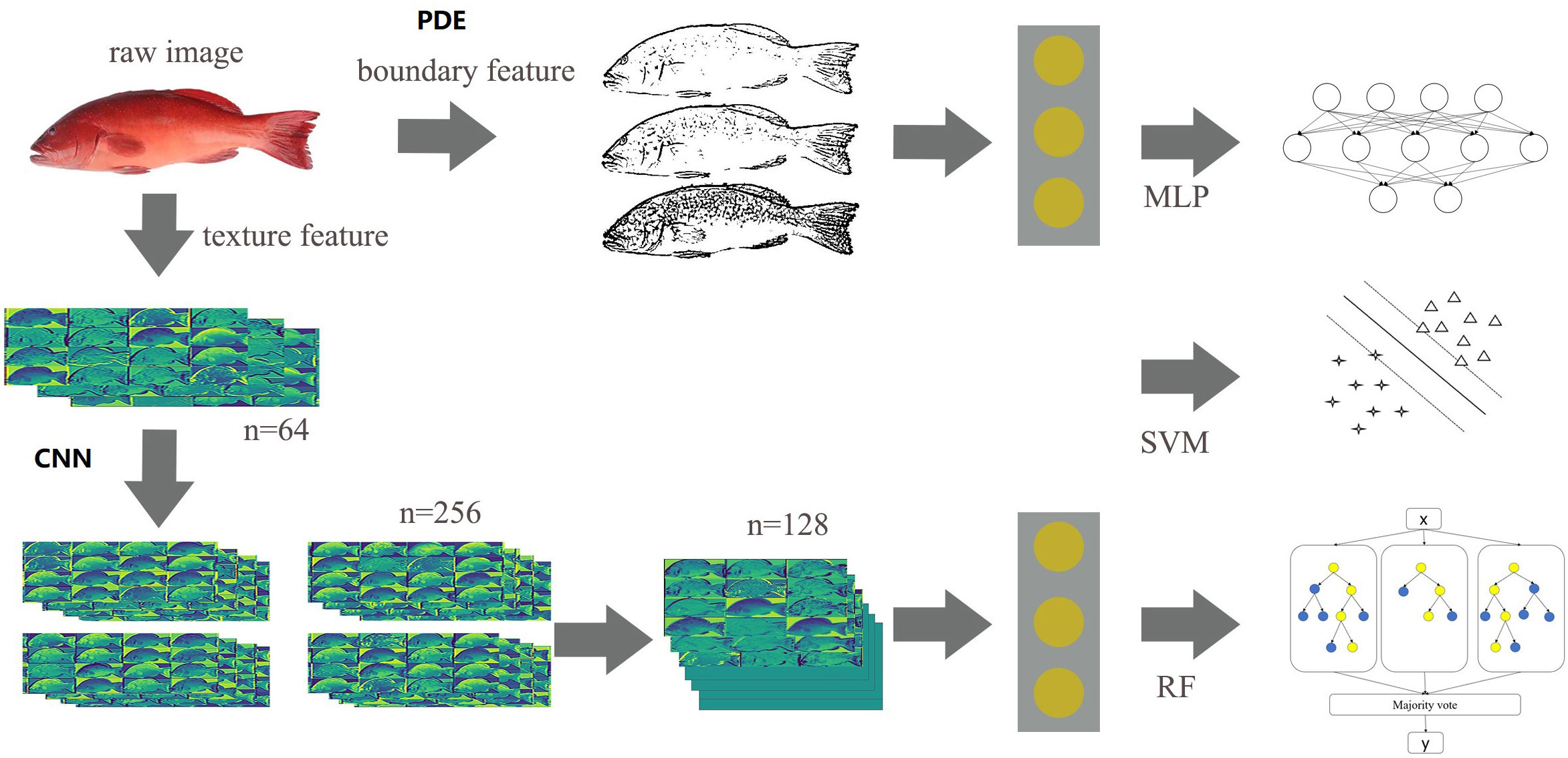
Figure 1 The essential architecture of our method for fully automated segmentation and identification of P. leopardus.

2.4 Model assessment indicators

In a multi-classification task, there are differences in the predicting ability of the model for different categories, and there may be category imbalance in the predicting results. Since the accuracy rate simply calculates the ratio of the number of correctly predicted samples to the total number of samples, ignoring the predicting ability of the model for different categories, it is hard to objectively measure the predicting effect of the model. In order to measure the model’s comprehensive predicting ability for each category, the accuracy for each category should be taken into account, so the Precise, Recall and Macro-F1 Score are selected as evaluation indicators (Zhou et al., 2021). The calculation method is as follows.

True Positives (TP): all cases where we have predicted YES and the actual result was YES. True Negatives (TN): all cases where we have predicted NO and the actual result was NO. False Positives (FP): all cases where prediction was YES, but the actual result was NO (‘Type I error’). False Negatives (FN): all cases where prediction was NO, but the actual result was YES (‘Type II error’).

Precision is the proportion of positive samples that are correctly predicted out of all samples that are predicted to be positive:

$$\text{Precision}=\frac{\text{TP}}{\text{TP}+\text{FP}}$$

Recall is the proportion of positive samples that are correctly predicted out of all actual positive samples (including the positive samples that were predicted incorrectly).

$$\text{Recall}=\frac{\text{TP}}{\text{TP}+\text{TN}}$$

F1-Score is the harmonic mean of precision and recall.

$$\text{F}1=\frac{2\times \text{Precision}\times \text{Recall}}{\text{Precision}+\text{Recall}}$$

Macro-F1 is the mean of F1-Score for each category, where N is the total number of categories.

$$\text{Macro F}1=\frac{{\sum }_{\text{N}}^{\text{i}}\text{F}{1}_{\text{i}}}{\text{N}}$$

2.5 Software and hardware environment

In this study, the Python 3.8.10 environment was used with the scikit-image library for feature extraction, the scikit-learn 0.24.0 library for principal component analysis and the construction of random forest and support vector machine models, and the tensorflow 2.3.1 library for CNN-based feature extraction and the training of multilayer perceptrons. The tsne library was used to accomplish the t-SNE downscaling and visualization in the R 4.1.1 environment.

3 Results

3.1 PDE-based feature extraction

The results of the illustrative segmentation of P. leopardus using the PDE multiscale decomposition method with different scale parameters are shown in Figure 2. Obviously, the camera image can be used for good segmentation with the selection of more growth rings of body shape. Meanwhile, the segmentation of shape contours in the image can be still detected even though the original image was degraded by some body color; hence, our segmentation method was robust in noise and color.

FIGURE 2

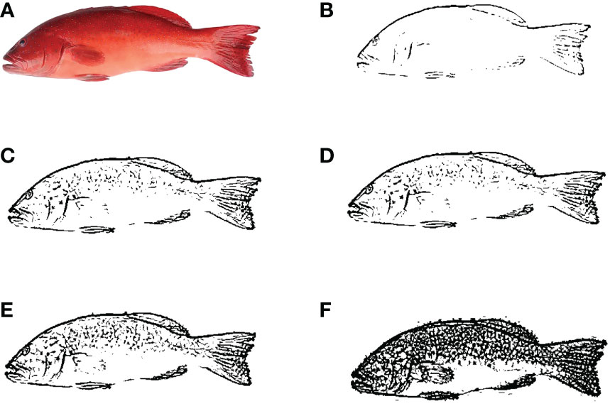
Figure 2 Segmentation results produced by multiscale hierarchical decomposition using PDE with λ0 = 0.01 and λi = λ02ⁱ (A) original image; (B–F) segmented image at scaling parameters λ1, λ2, λ3, λ4, and λ5, respectively.

3.2 CNN-based feature extraction

As shown in Figure 2, the PDE method can obtain more details of the shape of P. leopardus compared with the ResNet50 model of CNNs. By visualizing several convolutional layers in the ResNet50 model (Figure 1), we found that some kernels in different layers could distinguish smaller tubular and periodic structures in P. leopardus images, which made ResNet50 more effective in the extraction of texture details.

The shape and texture features obtained by PDE-based and CNN-based methods were visualized using the tSNE software (Figure 3). For the shape features obtained by PDE, the points of different categories overlapped each other and were difficult to distinguish (Figure 3A). While we found that the CNN-based texture features of the same individuals were gathered into a cluster, reflecting the intra-category consistency and inter-category dissimilarity, for example, individuals of 4, 5, 14, 15, 16, 17, 18, 19 in ResNet50 features (Figure 3B) and individuals of 5, 15, 19 in VGG19 features (Figure 3C). Features of the same individuals using the ResNet50 model were more likely to gather into clusters than the VGG19 features, suggesting that the ResNet50 feature may extract more small texture information from images than VGG19 features.

FIGURE 3

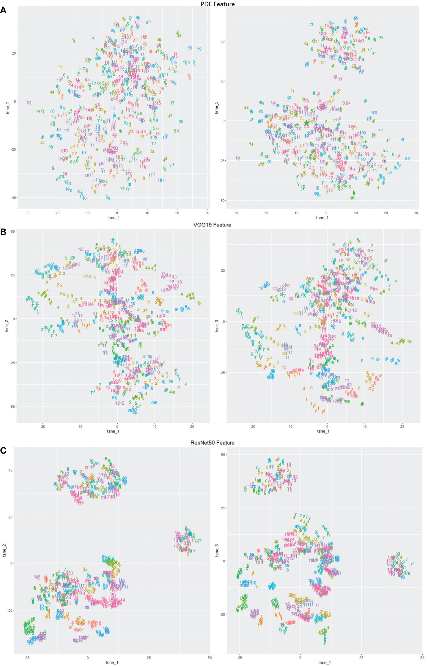
Figure 3 Visualization of feature-extraction methods (number labels in the range of 1~20 denote 20 individuals randomly sampled from all the P. leopardus) (A) PDE feature; (B) CNN ResNet50 feature; (C) CNN VGG19 feature.

3.3 Prediction performance of combinations with different features and classifiers

In this section, five-fold Cross-validation (5-fold CV) was used to assess the prediction performance of the different methods in the P. leopardus data set. For 5-fold CV, the data set was divided into five mutually exclusive subsets; four of five formed the estimation set (ES) for fitting input feature effects and the fifth subset was used as a test set (TS). Three methods (RF, SVM and MLP) were trained on the feature-extracted (PDE, VGG19 and ResNet50) datasets, and the traditional LeNet-5 convolutional neural network dataset of the 224*224-pixel images from the raw dataset, respectively (Table 1).

TABLE 1

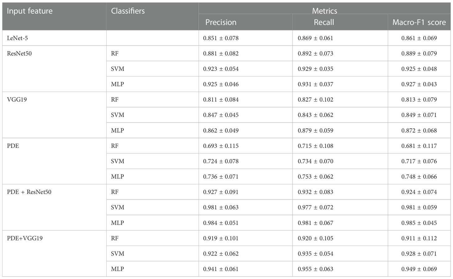
Table 1 Predictive accuracies obtained with different combination of features and classifiers by 5-fold CV.

Among the classifiers trained on the only PDE features for the dataset, PDE+ MLP achieved the best prediction (Macro-F1 Score 0.748 ± 0.066), followed by PDE + SVM (Macro-F1 Score 0.717 ± 0.076). The predicting performance of RF was poor with Macro-F1 score of only 0.681 ± 0.117. Compared with classifiers trained on PDE features, the simple CNN LeNet-5 with a simple structure had a significant improvement in the predicting effect with Macro-F1 score of 0.861 ± 0.069. For the deep CNN VGG19 features, VGG19+ MLP achieved the best prediction (Macro-F1 Score 0.872 ± 0.068) followed by VGG19 + SVM (Macro-F1 Score 0.849 ± 0.071) and VGG19 + RF (Macro-F1 Score 0.813 ± 0.079). Only VGG19 + MLP outperformed the simple LeNet-5 model (Macro-F1 Score 0.861 ± 0.069) with a Macro-F1 score increased about 0.011. After training on ResNet50 texture features, any classifier can achieve better predictions than any other combinations on VGG19 texture features. ResNet50 + MLP achieves the best prediction (Macro-F1 Score 0.927 ± 0.043) followed by ResNet50 + SVM (Macro-F1 Score 0.925 ± 0.048). It is interesting that SVM can also achieve similar performance on ResNet50-extracted features.

If we combined PDE shape features with ResNet50 or VGG19 text features to form a new feature set, any classifier can achieve better predictions than the feature set of PDE, VGG19, or ResNet50. In the PDE+ResNet50 dataset, the maximum accuracy was Macro-F1 Score 0.985 ± 0.045 for MLP. In the PDE+VGG19 dataset, the maximum accuracy was Macro-F1 Score 0.949 ± 0.069 for MLP. We, therefore, decided to take PDE+ResNet50+MLP and PDE+ResNet50+SVM as the experimental model to identify individuals in the following analyses.

3.4 Predictions effect of the model on training sets of different sizes

Due to the constraint of time and labor costs in actual application scenarios, it is often difficult to obtain large datasets. To refrain from the possible effect of the small dataset, it is necessary to investigate the predicting performance of the classifier on different size training sets to make a trade-off between the cost of dataset size and the predicted effect. The images of days 1-5, 1-10, 1-15, 1-20, 1-25, 1-30, 1-35,1-40 and 1-45 were taken from the ResNet50+ raw dataset and used for training MLP and SVM, respectively. The evaluation has two steps. Firstly, the prediction of these classifiers was estimated on the set of remaining images corresponding to their training set (e.g., for classifiers trained on images of days 1-5, the prediction was performed on images of days 6-50, and so on). Secondly, all classifiers trained on different periods of days were used to predict the images of days 46-50 (Figure 4).

FIGURE 4

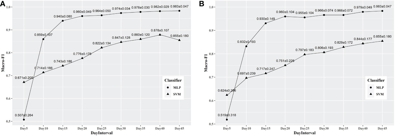
Figure 4 The results for prediction using classifiers trained by datasets with different size. (A) The results for prediction of the whole images of the rest days; (B) The results for prediction of the images of the 46^th -50^th days.

As shown in Figure 4, the Macro-F1 Scores of all the classifiers increase with the expansion of the sizes of training sets. When images of days 1-20 were used as the training set, models achieved relative high values of macro-F1 on all test sets with Macro-F1 Scores of 0.960 ± 0.049 for PDE+ResNet50+MLP to identify the individuals in images of the rest days and 0.960 ± 0.104 in images of days 46-50. When the size of the training set continues to enlarge, the curve of predicting effect goes steadily and changes slightly with the expansion of the training set. The highest Macro-F1 Score (0.983 ± 0.047) is achieved by PDE+ResNet50+MLP when using images of days 1-45 as the training set and images of days 46-50 as test sets. Furthermore, the Macro-F1 Score of PDE+ResNet50+MLP was higher than that of PDE+ResNet50+SVM in most sets of experiments except using images of 1-5 days as the training set.

3.5 Temporal tracking recognition of individuals on different time scales

In the actual scenario of breeding work, individuals need to be tracked continuously over a while. To investigate the tracking ability of the PDE+ResNet50 + MLP model, predicting the results of combination of the training set and test set for each individual on every day were extracted and summarized (Figure 5).

FIGURE 5

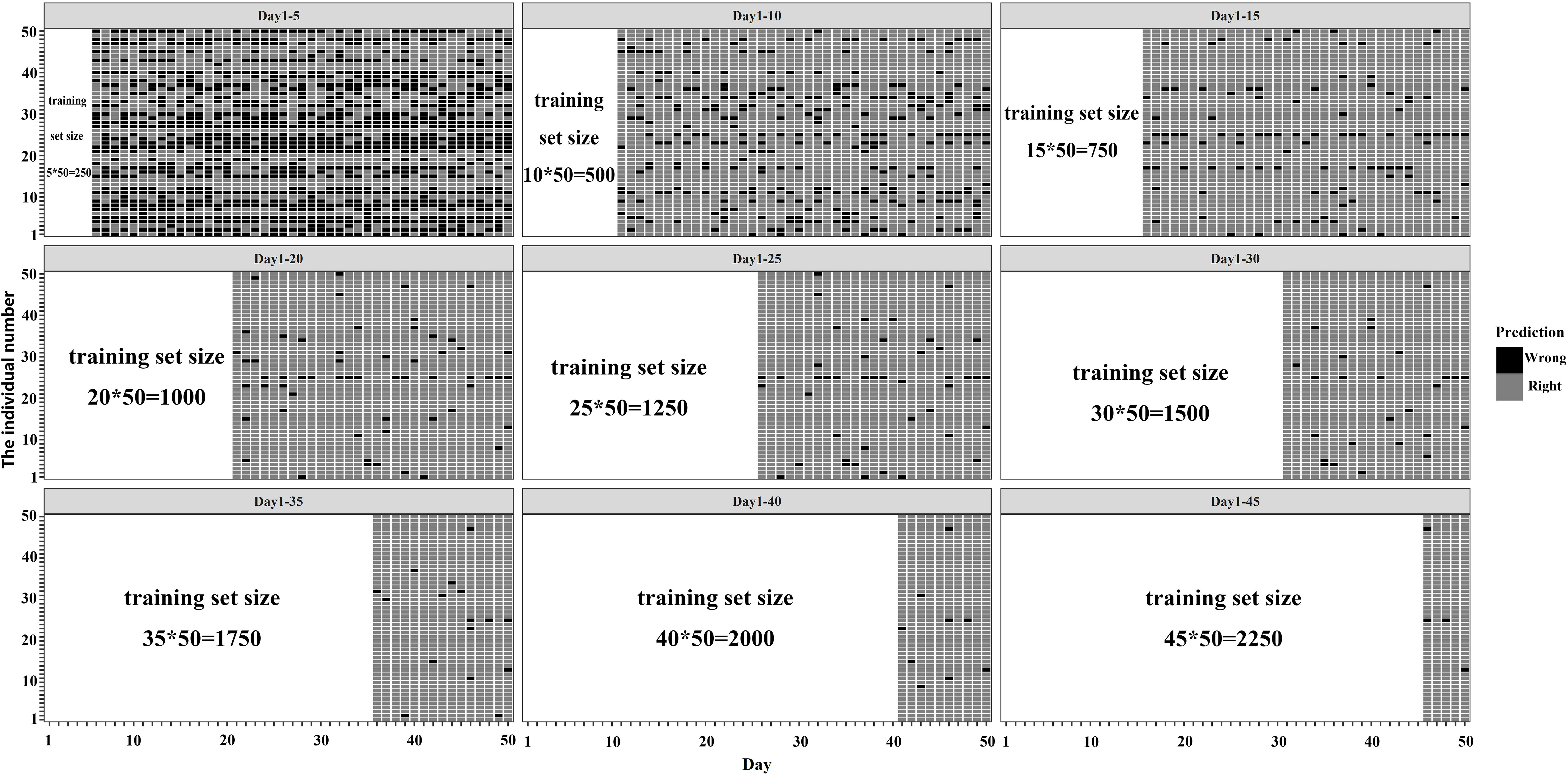
Figure 5 The result of tracking recognition of P. leopardus on different time scales.

When trained on images of days 1-5, 1-10, and 1-15, the size of the training set was small and the model performed poorly on some individuals. For example, when trained on images of days 1-5, the model performed poorly on most of the individuals. As the size of the training set increased, these hard-to-predict individuals were gradually correctly identified by the model. When trained with images of days 1-30, there were few individuals that were difficult to identify, and for some individuals, the model could achieve a 100% recognition rate.

To understand how well each individual was tracked, we treated it as a traceable individual with an error rate of less than or equal to 10%. Then the predicting effects for all individuals were counted according to the above criterion (Table 2). When the size of the training set was small, the number of traceable individuals increased with the increase of the size of the training set. When images of days 1-25 were used as the training set, the number of traceable individuals was 45, accounting for 90% of the total individuals, and the number of individuals that could be identified at a 100% recognition rate was 27. When images of days 1-30 were used as the training set, the proportion of traceable individuals reached 98%, and the number of individuals that could be 100% identified was 33.

TABLE 2

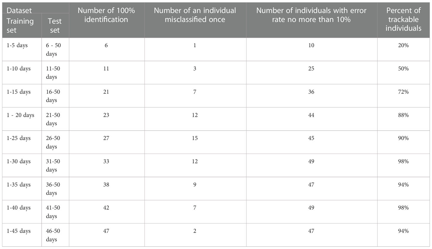
Table 2 The statistics for results of tracking recognition on different time scales.

4 Discussion

The approach described in this paper using image processing analytical methods, which are widely used in studies on ecology and evolution (Bolger et al., 2012), has demonstrated its powerful application in studies on non-invasive tagging methods for P. leopardus. The PDE-based and CNN-based image feature vector of each shape and texture structure, which is invariant against translation, rotation, scaling, and even modest distortion. As long as the feature pattern can be extracted from each image, the individuals can be effectively identified by using the RF, SVM and MLP classification of shape and texture features.

4.1 Advantages of deep convolutional neural networks in recognition of P. leopardus

To explore the feature extraction methods and machine learning models suitable for the recognition of P. leopardus, the PDE-based shape features, and CNN-based texture features were used for feature extraction, and then RF, SVM, and MLP were trained on the extracted features compared to the LeNet-5 model, an early convolutional neural network with fewer layers and a simple structure. The PDE + MLP obtained the best predictability with a Macro-F1 score of 0.748 ± 0.066 compared with PDE+RF and PDE+SVM on the raw dataset, while the ResNet50+MLP model achieved a Macro-F1 score of 0.927 ± 0.043, indicating that compared to the PDE-based image segmentation that had the relatively weak ability of feature extraction, ResNet50 extracted more details of features for individual imaged and achieved better recognition results. Various researchers are addressing the task of individual recognition in different way using traditional machine learning methods (Vaillant et al., 1994; Viola and Jones, 2001; Dollár et al., 2009) such as thresholding (Sivakumar and Murugesh, 2014), region growing (Gómez et al., 2007; Preetha et al., 2012), edge detection (Ma and Manjunath, 1997; Huang and Kuo, 2010; Wang et al., 2013), clustering (Celenk, 1990; Ali et al., 2006; Kavitha and Chellamuthu, 2010; Zheng et al., 2018), super-pixel (Li et al., 2012; Xie et al., 2019), etc. for years. PDE-based image multiscale decomposition belongs to edge detection method. Individual recognition research has also started to use the convolutional neural network (CNN) for better segmentation accuracy. That is why CNN is used successfully for individual recognition.

In this study, the CNN-based texture features included two categories: the features extracted by VGG19 and ResNet50. The VGG19 network has 16 layers of convolution layer (Simonyan and Zisserman, 2015), and the ResNet50 network has 49 layers of convolution layer (Savson et al., 2022). Among the three classifiers (RF, SVM, and MLP) trained with VGG19 features, VGG19 + MLP achieved the highest Macro-F1 score (0.872 ± 0.068), with an improvement of ~0.011 compared to LeNet-5 (0.861 ± 0.069). Our result is consistent with the conclusion in (He et al., 2016) that the accuracy of convolutional neural networks (CNNs) has been continuously improving. For example, the very deep VGG models, which have witnessed great success in a wide range of recognition tasks. In this study, when trained on a small dataset of 50 individuals, VGG19 or ResNet50 can better characterize the variability among individuals than LeNet-5 due to the deeper convolutional layers. Trained on the raw dataset, ResNet50+MLP achieved an improvement of ~0.055 compared to VGG19+MLP, indicating that the depth of the convolution layers in the ResNet50 network is enough for fully extracting the image features of P. leopardus. It is generally believed that by stacking multi-layer convolution kernels, the deep convolutional neural network allows the model to capture higher-dimensional and abstract features, including invisible high-frequency features that are traditionally considered noise (Krizhevsky et al., 2012). Thus, we purposed to use the ResNet50 to capture the patterns on the surface of P. leopardus.

Combined PDE-based and CNN-based features, PDE+ResNet50+MLP achieved the best prediction and PDE+ ResNet50+SVM got the suboptimal prediction, which are both better than those achieved by ResNet50+MLP and ResNet50+SVM trained on the same dataset. These results indicated that when the size of the training set was small, the CNN had difficulty in capturing more details of the shape features of P. leopardus. The PDE-based features generated by PDE multiscale decomposition contained a series of segmentation results at varying image resolutions of shape pattern details at different levels. This process performed an iterative segmentation at an increasing image resolution in each step, and thus detected much smaller patterns of shape. It was exactly because the PDE-based features added more shape features for the CNN-based features to identify the individuals more effectively. This result also suggested that CNNs with some image segmentation methods may be more well-suited for individual recognition when the size of the dataset is small compared to just using CNNs.

4.2 Prediction at different time scales determine the optimal dataset size

In practical applications, due to the limited time available for collecting image data of the P. leopardus, it is usually hard for researchers to obtain enough data, so a trade-off between data volume and predicting effect is needed. Thus, the whole dataset was divided at different ratios to simulate the training set on different time scales, which were used as the training set to train the classifier and the remaining images as the test set for prediction. When using images of days 1-20 (i.e., 20 images per individual, 1000 images in total) as the training set, better results could be obtained (0.960 ± 0.049). Then the curve of the Macro-F1 changed slightly as the size of the training set increased. When trained on images of days 1-45, a remarkable improvement in predicting effect was obtained (0.983 ± 0.047). Since the test set was small, which only had images from days 46-50 when using images from days 1-45 as the training dataset, the model may have a higher recognition rate for some specific individuals coincidently.

After fixing the test set to images of 46-50 days, the predicting effect of the classifiers trained on a series of image subsets of 1-45 days, compared with the image set of 1-45 days. The results showed that the average Macro-F1 score increased with the increasing subset size for the models. It then plateaued when using images of days 1-20 for training and more selected days. The predicting effect slight increased training with images of days 1-40 and days 1-45, which may be a serendipitous result caused by the small test set. In addition, because the images faithfully reflect a continuous morphological change of P. leopardus over time, the images of days 1-45 were temporal continuity with the test set of days 46-50, which might be another reason for the models to achieve the above best prediction.

4.3 Reliability of CNN-based recognition methods in long-term tracking

In the breeding work, breeders require individuals to be traceable for a long time using tagging methods, so it is necessary to ensure that the CNN-based method can achieve a comparatively high correction identification ratio of individuals for a continuous period. In our tracking experiments, we found that the performance of predicting effects showed large differences for some individuals. For example, the CNN-based method had a poor predicting effect on some individuals using small-size training sets, probably because the shape and texture features of these individuals were more similar to each other. If we expanded the training set, the model performed highly accurate recognition for these hard-to-identify individuals, showing that the CNN-based method needs large numbers of training images to obtain temporal-stable features for individual long-term tracking.

Most of the traditional tagging methods involve puncturing and destroying the body wall of P. leopardus, which can easily make them die due to wound ulceration. Meanwhile, the retention rate of the label fluctuates greatly due to the choice of the labeling tool, the experimental individual, and the operation methods. Generally speaking, the retention rate for one month is between 50% and 80%. The above two types of problems make it difficult to apply traditional tagging methods to the tagging work of aquatic animal breeding (Jepsen et al., 2015). Our method can also save time and cost less in comparison with molecular methods for the individual tracking, especially in a large population. For 100 individual samples, it would take approximately 14 days for good identification with the traditional molecular methods (Wang, 2016). In addition, these methods are generally laborious and time-consuming and sometimes require invasive operations that need a relatively large amount of sample materials, which would require the sacrifice of animals under study to ensure a sufficient amount of DNA for individual recognition (Mao et al., 2013). However, our method can achieve a high-throughput operation with aid of an ordinary digital camera, and even mobile phones and can reduce the workload to just less than 1 hrs. Therefore, we would propose that the use of CNN-based image recognition method has a great applying potential in the tagging work for P. leopardus.

4.4 Possible improving directions of model

In this study, the CNNs were trained on images of 50 days, which were randomly selected in the period. The sample size was relatively sufficient for training. However, in the actual breeding work, there are often more individuals. It is necessary to increase individuals in the subsequent study to explore the upper limit of the individuals that can be classified by the CNN method to meet the actual needs. Fortunately, many multiclassification models are now available, and perform well. Although the CNN approach outlined above has great potential, there are several outstanding challenges with applying CNNs to a wider spectrum of problems. One important obstacle is the large amount of training data required by CNNs. This challenge includes both the generation of large labeled training examples and time- and memory-efficient training with these large examples given limited computational resources. Fortunately, continued improvements in simulation speed and the efficiency of CNN training (Chilimbi et al., 2014; Urs et al., 2017) are mitigating this problem.

Another challenge with the application of CNNs is that their performance can be sensitive to network architecture (Szegedy et al., 2015). There is no underlying theory for selecting optimal network architecture, though improved architectures are sure to continue to arise, and automated methods exist for optimizing the many hyperparameters of a given architecture (Snoek et al., 2012). Though we uncover some promising CNN architectures for the recognition of P. leopardus, we suspect that substantial improvements can still be made. Meanwhile, length calibrators (e.g., rulers) can be added to the field of view for photograph, so that the difference in relative size among individuals can be involved in the dataset, which may improve the performance of model in the temporal tracking task. Furthermore, if more lightweight network architectures such as MobileNets (Li et al., 2012) are used, it is promising to deploy the recognition systems on mobile device as applications to enable mobile and real-time recognition of P. leopardus.

5 Conclusion

In this study, a dataset involving images of 50 P. leopardus individuals was obtained by continuous photography in 50 consecutive days. Then we performed prediction using different classifiers with different feature extraction methods and compare the predicting effect on the dataset. The results shows that the feature extraction method based on deep CNN model ResNet50 with PDE-based multiscale decomposition segmentation method performed well in the recognition task of P. leopardus. The prediction results on training sets of different sizes show that the model achieves satisfactory prediction results when the number of images per individuals in training set reaches 20. Temporal tracking recognition experiments on different time scales showed that the deep CNN model ResNet50 with PDE-based segmentation method can recognize individuals over a longer time span with better accuracy than other invasive tagging methods. The results of this study will provide an important reference for the development of non-invasive tagging methods based on deep learning and the characterization of complex traits of P. leopardus. In the future, we will increase the population to further verify our conclusion.

Data availability statement

The raw data supporting the conclusions of this article will be made available by the authors, without undue reservation.

Ethics statement

The animal study was reviewed and approved by Institutional Animal Care and Use Committee of Ocean University of China.

Author contributions

All authors listed have made a substantial, direct, and intellectual contribution to the work, and approved it for publication.

Funding

We acknowledged the National Key Research and Development Program of China (2022YFD2400501), the Key R&D Project of Hainan Province (ZDYF2021XDNY133), National Natural Science Foundation of China (32072976), Sanya Yazhou Bay Science and Technology City (SKJCKJ-2019KY01), and the China Postdoctoral Science Foundation (2021703030).

Conflict of interest

The authors declare that the research was conducted in the absence of any commercial or financial relationships that could be construed as a potential conflict of interest.

The handling editor HZ declared a shared affiliation with the authors at the time of review.

Publisher’s note

All claims expressed in this article are solely those of the authors and do not necessarily represent those of their affiliated organizations, or those of the publisher, the editors and the reviewers. Any product that may be evaluated in this article, or claim that may be made by its manufacturer, is not guaranteed or endorsed by the publisher.

References

Ali M. A., Dooley L. S., Karmakar G. C. (2006). “Object based image segmentation using fuzzy clustering,” in 2006 IEEE International Conference on Acoustics Speech and Signal Processing Proceedings, Toulouse, France: IEEE. doi: 10.1109/ICASSP.2006.1660290

CrossRef Full Text | Google Scholar

Bolger D. T., Morrison T. A., Vance B., Lee D., Farid H. (2012). A computer-assisted system for photographic mark–recapture analysis. Methods Ecol. Evol. 3 (5), 813–822. doi: 10.1111/j.2041-210X.2012.00212.x

CrossRef Full Text | Google Scholar

Celenk M. (1990). A color clustering technique for image segmentation. Comput. Vis. Graph. Image Process 52 (2), 145–170. doi: 10.1016/0734-189X(90)90052-W

CrossRef Full Text | Google Scholar

Chaudhuri S., Chatterjee S., Katz N., Nelson M., Goldbaum M. (1989). Detection of blood vessels in retinal images using two-dimensional matched filters. IEEE. Trans. Med. Imaging 8 (3), 263–269. doi: 10.1109/42.34715

PubMed Abstract | CrossRef Full Text | Google Scholar

Chilimbi T., Suzue Y., Apacible J., Kalyanaraman K. (2014). “Project adam: Building an efficient and scalable deep learning training system,” in 11th USENIX Symposium on Operating Systems Design and Implementation (OSDI 14) (Berkeley, CA, USA: USENIX Association) 571–582. doi: 10.1108/01439911111122716

CrossRef Full Text | Google Scholar

Cortes C., Vapnik V. (1995). Support-vector networks. Mach. Learn. 20 (3), 273–297. doi: 10.1007/BF00994018

CrossRef Full Text | Google Scholar

Døving K., Westerberg H., Johnsen P. (2011). Role of olfaction in the behavioral and neuronal responses of Atlantic salmon, Salmo salar, to hydrographic stratification. Can. J. Fish. Aquat. Sci. 42, 1658–1667. doi: 10.1139/f85-207

CrossRef Full Text | Google Scholar

Dollár P., Tu Z., Perona P., Belongie S. (2009). “Integral channel features,” in British Machine Vision Conference. (London, UK:BMVC Press) 91.1–91.11. doi: 10.5244/C.23.91

CrossRef Full Text | Google Scholar

Fearnbach H., Durban J., Parsons K., Claridge D. (2012). Photographic mark-recapture analysis of local dynamics within an open population of dolphins. Ecol. Appl. 22 (5), 1689–1700. doi: 10.1890/12-0021.1

PubMed Abstract | CrossRef Full Text | Google Scholar

Forcada J., Aguilar A. (2000). Use of photographic identification in capture-recapture studies of mediterranean monk seals. Mar. Mammal. Sci. 16 (4), 767–793. doi: 10.1111/j.1748-7692.2000.tb00971.x

CrossRef Full Text | Google Scholar

Gómez O., González J. A., Morales E. F. (2007). “Image segmentation using automatic seeded region growing and instance-based learning,” in Progress in pattern recognition, image analysis and applications. Eds. Rueda L., Mery D., Kittler J. (Berlin Heidelberg: Springer), 192–201. doi: 10.1007/978-3-540-76725-1_21

CrossRef Full Text | Google Scholar

He K., Zhang X., Ren S., Sun J. (2016). “Deep residual learning for image recognition,” in 2016 IEEE Conference on Computer Vision and Pattern Recognition (CVPR), Las Vegas, NV, USA: IEEE. 770–778. doi: 10.1109/CVPR.2016.90

CrossRef Full Text | Google Scholar

Hinch S. G., Standen E. M., Healey M. C., Farrell A. P. (2002). Swimming patterns and behaviour of upriver-migrating adult pink (Oncorhynchus gorbuscha) and sockeye (O. nerka) salmon as assessed by EMG telemetry in the Fraser river, British Columbia, Canada. Hydrobiologia 483 (1), 147–160. doi: 10.1023/A:1021327511881

CrossRef Full Text | Google Scholar

Huang Y. R., Kuo C. M. (2010). “Image segmentation using edge detection and region distribution,” in 2010 3rd International Congress on Image and Signal Processing, Yantai, China: IEEE. 1410–1414. doi: 10.1109/CISP.2010.5646352

CrossRef Full Text | Google Scholar

Jepsen N., Thorstad E. B., Havn T., Lucas M. C. (2015). The use of external electronic tags on fish: an evaluation of tag retention and tagging effects. Anim. Biotelemetry. 3 (1), 49. doi: 10.1186/s40317-015-0086-z

CrossRef Full Text | Google Scholar

Kamilaris A., Prenafeta-Boldú F. X. (2018). A review of the use of convolutional neural networks in agriculture. J. Agric. Sci. 156 (3), 312–322. doi: 10.1017/S0021859618000436

CrossRef Full Text | Google Scholar

Karanth U., Nichols J. D. (1998). Estimation of tiger densities in India using photographic captures and recaptures. Ecology 79 (8), 2852–2862. doi: 10.1890/0012-9658(1998)079[2852:EOTDII]2.0.CO;2

CrossRef Full Text | Google Scholar

Kavitha A. R., Chellamuthu C. (2010). Implementation of gray-level clustering algorithm for image segmentation. Procedia. Comput. Sci. 2, 314–320. doi: 10.1016/j.procs.2010.11.041

CrossRef Full Text | Google Scholar

Krizhevsky A., Sutskever I., Hinton G. E. (2012). “ImageNet classification with deep convolutional neural networks,” in NIPS'12: Proceedings of the 25th International Conference on Neural Information Processing Systems, New York, United States: Curran Associates Inc. 1097–1105. doi: 10.1145/3065386

CrossRef Full Text | Google Scholar

Langtimm C. A., Beck C. A., Edwards H. H., Fick-Child K. J., Ackerman B. B., Barton S. L., et al. (2004). Survival estimates for Florida manatees from the photo-identification of individuals. Mar. Mammal. Sci. 20 (3), 438–463. doi: 10.1111/j.1748-7692.2004.tb01171.x

CrossRef Full Text | Google Scholar

LeCun Y., Bengio Y., Hinton G. (2015). Deep learning. Nature 521 (7553), 436–444. doi: 10.1038/nature14539

PubMed Abstract | CrossRef Full Text | Google Scholar

Lecun Y., Bottou L., Bengio Y., Haffner P. (1998). Gradient-based learning applied to document recognition. Proc. IEEE. 86 (11), 2278–2324. doi: 10.1109/5.726791

CrossRef Full Text | Google Scholar

Linderman G. C., Rachh M., Hoskins J. G., Steinerberger S., Kluger Y. (2019). Fast interpolation-based t-SNE for improved visualization of single-cell RNA-seq data. Nat. Methods 16 (3), 243–245. doi: 10.1038/s41592-018-0308-4

PubMed Abstract | CrossRef Full Text | Google Scholar

Li Z., Wu X. M., Chang S. F. (2012). “Segmentation using superpixels: A bipartite graph partitioning approach,” in 2012 IEEE Conference on Computer Vision and Pattern Recognition, Providence, RI, USA: IEEE. doi: 10.1109/CVPR.2012.6247750

CrossRef Full Text | Google Scholar

Ma W. Y., Manjunath B. S. (1997). “Edge flow: A framework of boundary detection and image segmentation,” in Proceedings of IEEE Computer Society Conference on Computer Vision and Pattern Recognition, San Juan, PR, USA: IEEE. 744–749. doi: 10.1109/CVPR.1997.609409

CrossRef Full Text | Google Scholar

Mao J., Lv J., Miao Y., Sun C., Hu L., Zhang R., et al. (2013). Development of a rapid and efficient method for non-lethal DNA sampling and genotyping in scallops. PLoS. One 8 (7), e68096. doi: 10.1371/journal.pone.0068096

PubMed Abstract | CrossRef Full Text | Google Scholar

Ogura M., Ishida Y. (1995). Homing behavior and vertical movements of four species of pacific salmon (Oncorhynchus spp.) in the central Bering Sea. Can. J. Fish. Aquat. Sci. 52 (3), 532–540. doi: 10.1139/f95-054

CrossRef Full Text | Google Scholar

Preetha M. M. S. J., Suresh L. P., Bosco M. J. (2012). “Image segmentation using seeded region growing",” in 2012 International Conference on Computing, Electronics and Electrical Technologies (ICCEET), Nagercoil, India: IEEE. 576–583. doi: 10.1109/ICCEET.2012.6203897

CrossRef Full Text | Google Scholar

Quinn T. P., Terhart B. A., Groot C. (1989). Migratory orientation and vertical movements of homing adult sockeye salmon, Oncorhynchus nerka, in coastal waters. Anim. Behav. 37, 587–599. doi: 10.1016/0003-3472(89)90038-9

CrossRef Full Text | Google Scholar

Raab T., Madhav M. S., Jayakumar R. P., Henninger J., Cowan N. J., Benda J. (2022). Advances in non-invasive tracking of wave-type electric fish in natural and laboratory settings. Front. Integr. Neurosci. 16. doi: 10.3389/fnint.2022.965211

PubMed Abstract | CrossRef Full Text | Google Scholar

Redmon J., Divvala S., Girshick R., Farhadi A. (2016). “You only look once: unified, real-time object detection,” in 2016 IEEE Conference on Computer Vision and Pattern Recognition (CVPR), Las Vegas, NV, USA: IEEE. 779–788. doi: 10.1109/CVPR.2016.91

CrossRef Full Text | Google Scholar

Reed J. Z., Tollit D. J., Thompson P. M., Amos W. (1997). Molecular scatology: the use of molecular genetic analysis to assign species, sex and individual identity to seal faeces. Mol. Ecol. 6 (3), 225–234. doi: 10.1046/j.1365-294x.1997.00175.x

PubMed Abstract | CrossRef Full Text | Google Scholar

Rimmer M. A., Glamuzina B. (2019). A review of grouper (Family serranidae: Subfamily epinephelinae) aquaculture from a sustainability science perspective. Rev. Aquac. 11 (1), 58–87. doi: 10.1111/raq.12226

CrossRef Full Text | Google Scholar

Rudin L. I., Osher S., Fatemi E. (1992). Nonlinear total variation based noise removal algorithms. Phys. D. 60 (1), 259–268. doi: 10.1016/0167-2789(92)90242-F

CrossRef Full Text | Google Scholar

Savson D. J., Zenilman S. S., Smith C. R., Daugherity E. K., Singh B., Getchell R. G. (2022). Comparison of alfaxalone and tricaine methanesulfonate immersion anesthesia and alfaxalone residue clearance in rainbow trout (Oncorhynchus mykiss). Comp. Med. 72 (3), 181–194. doi: 10.30802/aalas-cm-22-000052

PubMed Abstract | CrossRef Full Text | Google Scholar

Shi L., Ye S. W., Zhu H., Ji X., Wang J. C., Liu C. A., et al. (2022). The spatial-temporal distribution of fish in lake using acoustic tagging and tracking method. Acta Hydrobiol. Sin. 46 (5), 611–620. doi: 10.7541/2022.2021.004

CrossRef Full Text | Google Scholar

Simonyan K., Zisserman A. (2015). Very deep convolutional networks for large-scale image recognition. CoRR, abs/1409.1556, arXiv:1409.1556. doi: 10.48550/arXiv.1409.1556

CrossRef Full Text | Google Scholar

Sivakumar V., Murugesh V. (2014). “A brief study of image segmentation using thresholding technique on a noisy image",” in International Conference on Information Communication and Embedded Systems (ICICES2014), Chennai, India: IEEE. 1–6. doi: 10.1109/ICICES.2014.7034056

CrossRef Full Text | Google Scholar

Šmejkal M., Bartoň D., Děd V., Souza A. T., Blabolil P., Vejřík L., et al. (2020). Negative feedback concept in tagging: Ghost tags imperil the long-term monitoring of fishes. PLoS. One 15 (3), e0229350. doi: 10.1371/journal.pone.0229350

PubMed Abstract | CrossRef Full Text | Google Scholar

Snoek J., Larochelle H., Adams R. P. (2012). “Practical Bayesian optimization of machine learning algorithms,” in NIPS'12: Proceedings of the 25th International Conference on Neural Information Processing Systems, New York, United States: Curran Associates Inc. 2951–2959. doi: 10.48550/arXiv.1206.2944

CrossRef Full Text | Google Scholar

Stateczny A., Uday Kiran G., Bindu G., Ravi Chythanya K., Ayyappa Swamy K. (2022). Spiral search grasshopper features selection with VGG19-ResNet50 for remote sensing object detection. Remote. Sens. 14(21), 5398. doi: 10.3390/rs14215398

CrossRef Full Text | Google Scholar

Sulak K. J., Randall M. T., Edwards R. E., Summers T. M., Luke K. E., Smith W. T., et al. (2009). Defining winter trophic habitat of juvenile gulf sturgeon in the suwannee and Apalachicola rivermouth estuaries, acoustic telemetry investigations. J. Appl. Ichthyol. 25 (5), 505–515. doi: 10.1111/j.1439-0426.2009.01333.x

CrossRef Full Text | Google Scholar

Szegedy C., Wei L., Yangqing J., Sermanet P., Reed S., Anguelov D., et al. (2015). Going deeper with convolutions in 2015 IEEE Conference on Computer Vision and Pattern Recognition (CVPR), (Boston, MA, USA: IEEE). 1–9. doi: 10.1109/CVPR.2015.7298594

CrossRef Full Text | Google Scholar

Urs K., Webb T. J., Wang X., Nassar M., Arjun K., Bansal, et al. (2017). “Flexpoint: an adaptive numerical format for efficient training of deep neural networks,” in NIPS'17: Proceedings of the 31st International Conference on Neural Information Processing Systems, New York, United States: Curran Associates Inc. doi: 10.48550/arXiv.1711.02213

CrossRef Full Text | Google Scholar

Vaillant R., Monrocq C., Lecun Y. (1994). Original approach for the localization of objects in images. IEE. P-VIS. Image. Sign. 141 (4), 245–250. doi: 10.1049/ip-vis:19941301

CrossRef Full Text | Google Scholar

Viola P., Jones M. (2001). “Rapid object detection using a boosted cascade of simple features,” in Proceedings of the 2001 IEEE Computer Society Conference on Computer Vision and Pattern Recognition, Kauai, HI, USA: IEEE. I–I. doi: 10.1109/CVPR.2001.990517

CrossRef Full Text | Google Scholar

Wang J. (2016). Individual identification from genetic marker data: developments and accuracy comparisons of methods. Mol. Ecol. Resour. 16 (1), 163–175. doi: 10.1111/1755-0998.12452

PubMed Abstract | CrossRef Full Text | Google Scholar

Wang Y., Ji G., Lin P., Trucco E. (2013). Retinal vessel segmentation using multiwavelet kernels and multiscale hierarchical decomposition. Pattern. Recognit. 46 (8), 2117–2133. doi: 10.1016/j.patcog.2012.12.014

CrossRef Full Text | Google Scholar

Watanabe Y. Y., Goldman K. J., Caselle J. E., Chapman D. D., Papastamatiou Y. P. (2015). Comparative analyses of animal-tracking data reveal ecological significance of endothermy in fishes. Proc. Natl. Acad. Sci. 112 (19), 6104–6109. doi: 10.1073/pnas.1500316112

CrossRef Full Text | Google Scholar

Welch D. W., Ward B. R., Batten S. D. (2004). Early ocean survival and marine movements of hatchery and wild steelhead trout (Oncorhynchus mykiss) determined by an acoustic array: Queen Charlotte strait, British Columbia. Deep. Sea. Res. Part II. 51 (6), 897–909. doi: 10.1016/j.dsr2.2004.05.010

CrossRef Full Text | Google Scholar

Williams B. K., Nichols J. D., Conroy M. J. (2002). Analysis and management of animal populations: modeling, estimation and decision making (San Diego, CA: Academic Press).

Google Scholar

Xia S., Sun J., Li M., Zhao W., Zhang D., You H., et al. (2020). Influence of dietary protein level on growth performance, digestibility and activity of immunity-related enzymes of leopard coral grouper, Plectropomus leopardus (Lacépèd 1802). Aquacult. Nutr. 26 (2), 242–247. doi: 10.1111/anu.12985

CrossRef Full Text | Google Scholar

Xie X., Xie G., Xu X., Cui L., Ren J. (2019). Automatic image segmentation with superpixels and image-level labels. IEEE. Access. 7, 10999–11009. doi: 10.1109/ACCESS.2019.2891941

CrossRef Full Text | Google Scholar

Yang Y., Wu L. N., Chen J. F., Wu X., Xia J. H., Meng Z. N., et al. (2020). Whole-genome sequencing of leopard coral grouper (Plectropomus leopardus) and exploration of regulation mechanism of skin color and adaptive evolution. Zool. Res. 41 (3), 328–340. doi: 10.24272/j.issn.2095-8137.2020.038

PubMed Abstract | CrossRef Full Text | Google Scholar

Yano A., Ogura M., Sato A., Sakaki Y., Ban M., Nagasawa K. (1996). Development of ultrasonic telemetry technique for investigating the magnetic of salmonids. Fish. Sci. 62 (5), 698–704. doi: 10.2331/fishsci.62.698

CrossRef Full Text | Google Scholar

Yoshua B. (2011). “Deep learning of resentations for unsupervised and transfer learning,” in UTLW'11: Proceedings of the 2011 International Conference on Unsupervised and Transfer Learning workshop, (Washington, USA: JMLR.org) 17–37.

Google Scholar

Zheng X., Lei Q., Yao R., Gong Y., Yin Q. (2018). Image segmentation based on adaptive K-means algorithm. Eurasip. J. Image. Video. Process 2018 (1), 68. doi: 10.1186/s13640-018-0309-3

CrossRef Full Text | Google Scholar

Zhou L., Zheng X., Yang D., Wang Y., Bai X., Ye X. (2021). Application of multi-label classification models for the diagnosis of diabetic complications. BMC. Med. Inform. Decis. Mak. 21 (1), 182. doi: 10.1186/s12911-021-01525-7

PubMed Abstract | CrossRef Full Text | Google Scholar

Zhuang X., Qu M., Zhang X., Ding S. (2013). A comprehensive description and evolutionary analysis of 22 grouper (perciformes, epinephelidae) mitochondrial genomes with emphasis on two novel genome organizations. PLoS. One 8 (8), e73561. doi: 10.1371/journal.pone.0073561

PubMed Abstract | CrossRef Full Text | Google Scholar