Development of a GNSS/INS buoy array in preparation for SWOT validation in Bass Strait

In preparation for validation of the swath-based altimetry mission (Surface Water Oceanography Topography, SWOT), we developed a buoy array, equipped with Global Navigation Satellite System/Inertial Navigation System, capable of accurately observing sea surface height (SSH), wave information and tropospheric delay. Here we present results from an 8-day trial deployment at five locations along a Sentinel-6 Michael Freilich (S6MF) ground track in Bass Strait. A triplet buoy group including two new buoys (Mk-VI) and a single predecessor (Mk-IV) were deployed in proximity to the historic Jason-series comparison point. SSH solutions compared against an in-situ mooring suggest the new buoys were working at an equivalent precision of ~1.5 cm to the previous design (MK-IV). At 10-km spacing along the S6MF track, the buoy array was shown to observe the progression of oceanographic and meteorological phenomena. Tidal analysis of the buoy array indicated moderate spatial variability in the shallow water tidal constituents, with differences in the instantaneous tidal height of up to ~0.2 m across the 40-km track. Further, tidal resonance within Bass Strait was observed to vary, most probably modulated by atmospheric conditions, yet only partially captured by an existing dynamic atmospheric correction product. A preliminary investigation into the spatial scale of the buoy error based on observed/inferred geostrophic currents with our present buoy array configuration suggests that the signal-noise ratio of the array became significant at 20-km spacing in Bass Strait. Finally, as an illustrative comparison between the buoy array and high resolution S6MF data, a single cycle was compared. The wet tropospheric delay observed by the S6MF radiometer exhibited some potential land contamination in the deployed area, while the 1-Hz and 20-Hz significant wave height from S6MF appeared within mission requirements. Generally good agreement between buoy and altimeter SSH was observed. However, subtle differences between the altimeter and the buoy sea level anomaly series warrants further investigation with additional cycles from a sustained deployment in the area. We conclude that the buoy array offers a useful geodetic tool to help quantify and understand intra-swath variability in the context of the SWOT mission.

1 Introduction

Developments in ocean altimetry continue to drive improved understanding of ocean and climate processes (Donlon et al., 2021). Sentinel 6 Michael Freilich (S6MF) was launched in November 2020 and for the first time operates under the high-resolution interleaved measurement approach (Donlon et al., 2021) allowing it to generate continuous full Synthetic Aperture Radar (SAR) output and achieve high quality high resolution (300 m) observations along the same reference track as the Jason satellite series. While some validation work via single-point based approaches (Haines et al., 2021; Watson et al., 2021) has begun, the improvements seen in the new SAR mission already demand improved performance from validation approaches.

The interferometric Surface Water Ocean Topography (SWOT) altimetry mission is scheduled for launch at the end of 2022. It will deliver a paradigm shift in ocean observations moving from nadir coverage over the water surface along track to swath-based observations. By design, it is expected to assist the oceanography community in the study of (sub-)meso-scale ocean processes, which is previously limited by the orbital track spacing (Morrow et al., 2019). As a result, even more strict validation requirements have been proposed (Esteban-Fernandez et al., 2017). Given the targeted ocean processes, SWOT validation calls for not only extension of precision from pointwise to spatial scales, but also qualification from the temporal perspective, in particular through the satellite initial 1-day repeat fast sampling phase.

In the context of preparing for SWOT, we extend a single buoy approach (Watson et al., 2003; Watson et al., 2011; Zhou et al., 2020) to a buoy array, with the intent to quantify and understand intra-swath variability. In this paper, we focus on presenting the development of a new Global Navigation Satellite System/Inertial Navigation System (GNSS/INS) buoy array concept which is capable of sustained deployment at chosen deployment locations. We assess the capabilities of this array via a trial 8-day deployment in Bass Strait. As a case study, we investigate signal and noise present over a ~40 km stripe (at 10 km spacing) along a S6MF track, centred at the historic Jason-series comparison point (hereinafter referred as JAS-CP or just JAS when there are multiple comparison points on the Jason track).

At the basis of this case study, we first examined the overarching precision of the new University of Tasmania/Integrated Marine Observing System Mark-VI (UTas/IMOS Mk-VI) buoy and compared it with the smaller predecessor (Mk-IV) – hereinafter referred to as the Mk-IV and Mk-VI buoys. With six new Mk-VI buoys and one Mk-IV buoy, we seek to understand the capability of the buoy array in measuring the spatial and temporal progression of key oceanic and atmospheric conditions. For comparison purposes, we also examined the derived in situ sea surface height/sea level anomaly (SSH/SLA), tropospheric delay and significant wave height (SWH) against the S6MF altimetry product from a single pass over the study region.

2 Study site

This study is centred on the JAS CP at the Bass Strait altimeter validation facility (Figure 1). Our buoy array instrumentation is deployed at 10 km intervals spanning 40 km along the S6MF pass 088. A combination of six new Mk-VI buoys and one predecessor Mk-IV buoy were deployed (Figure 1). A triplet buoy group including two Mk-VI and one Mk-IV were deployed at JAS CP to assess the performance of the two buoy designs. The water depth is quite consistent at ~48 m (JAS-20), ~51-52m (JAS-10, JAS CP) and ~47 m (JAS+10, JAS+20), where the JAS ± X site nomenclature refers to the along track distance in km from the JAS CP. Along the coast, Stanley GNSS site (STLY) and Rocky Cape GNSS site (RKCP) function as the reference stations for the buoy array for data processing, while further east the Burnie Tide Gauge (TG) provides additional observations for validation activities.

FIGURE 1

Figure 1 Configuration of the buoy array along Pass 88 at the Bass Strait validation facility. Land-based GNSS reference stations are shown in white. The Low-Resolution (LR) and High-Resolution (HR) waveform from Sentinel-6 is shown on the left and right side, respectively, (offset for readability) along track to qualitatively illustrate that the return waveform is relatively homogenous and of high quality without obvious land contamination at the buoy deployment locations (whereas closer to the coast and the Burnie TG, the quality of the waveform deteriorates quickly, in particular for LR – marked in the black dash rectangle box). An In-situ mooring including a bottom pressure sensor and a current-meter is co-located at JAS CP. The SWOT swath and nadir track for the fast sampling phase orbit shown in the background. The BXX nomenclature refers to the serial number for each buoy from the array.

3 Instrumentation

3.1 Buoy array

The Mk-IV buoy has been highly useful (Watson et al., 2011; Zhou et al., 2020) but was designed for short term deployment in relatively calm conditions. However, SWOT validation calls for sustained deployment and hence requires capability to endure higher sea states. To expand the power capacity, we have increased the size of the platform to enable the inclusion of solar panels. This allows us to extend the duration of a standard deployment from 48 hours up to multiple months. This process involved effectively scaling up the platform design and elevating the antenna height, making it more tolerant of dynamic ocean conditions.

To reduce the impact of external forcings on the buoy dynamics, and following a number of practical investigations in the past few years via an intermediate Mk-V prototype, we maintained the design of the cylindrical floats and payload. Further, in our anchor/float/tether system (Figure S1), the tether is aimed to be kept mostly horizontal to alleviate any vertical component in the drag induced by the current. Moreover, the new Mk-VI buoy also has an Inertial Measurement Unit (IMU) onboard to characterize platform orientations and potentially quantify any bias caused by buoy dynamics. Further details of the changes made from the Mk-IV to Mk-VI designed can be found in Table 1, while key features of Mk-VI design are shown in Figure 2.

TABLE 1

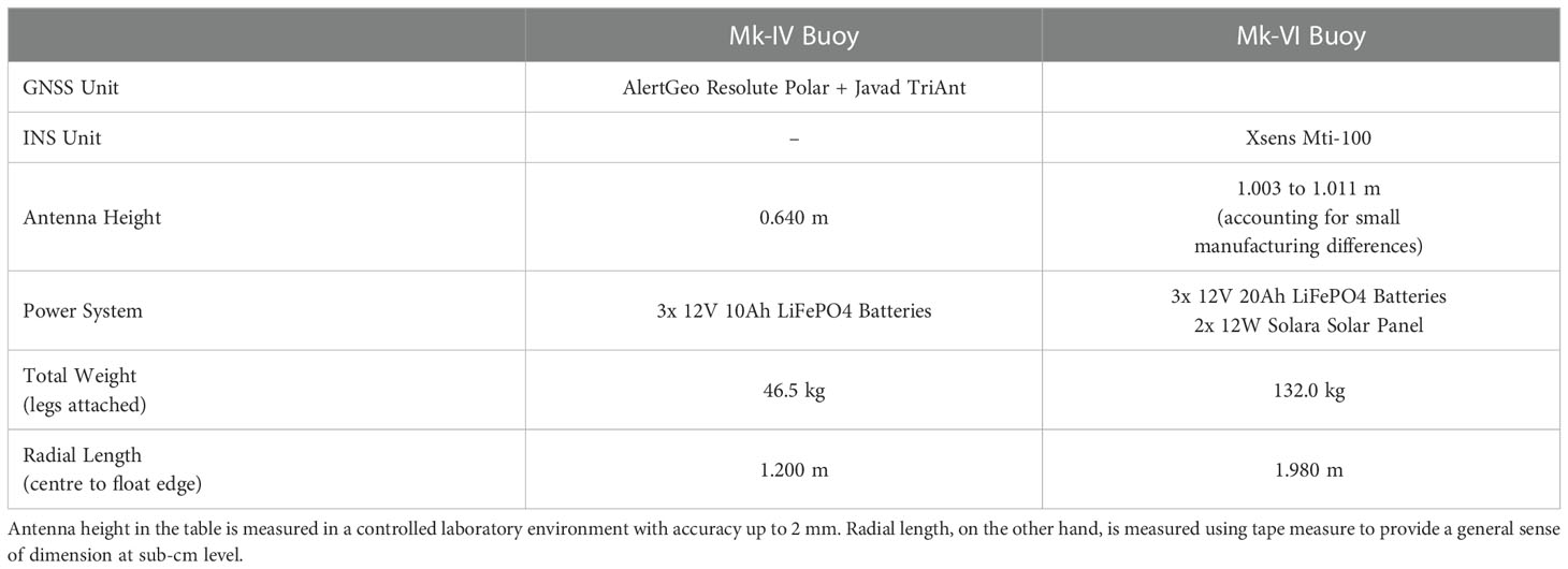
Table 1 Design difference between Mk-IV buoy and Mk-VI buoy.

FIGURE 2

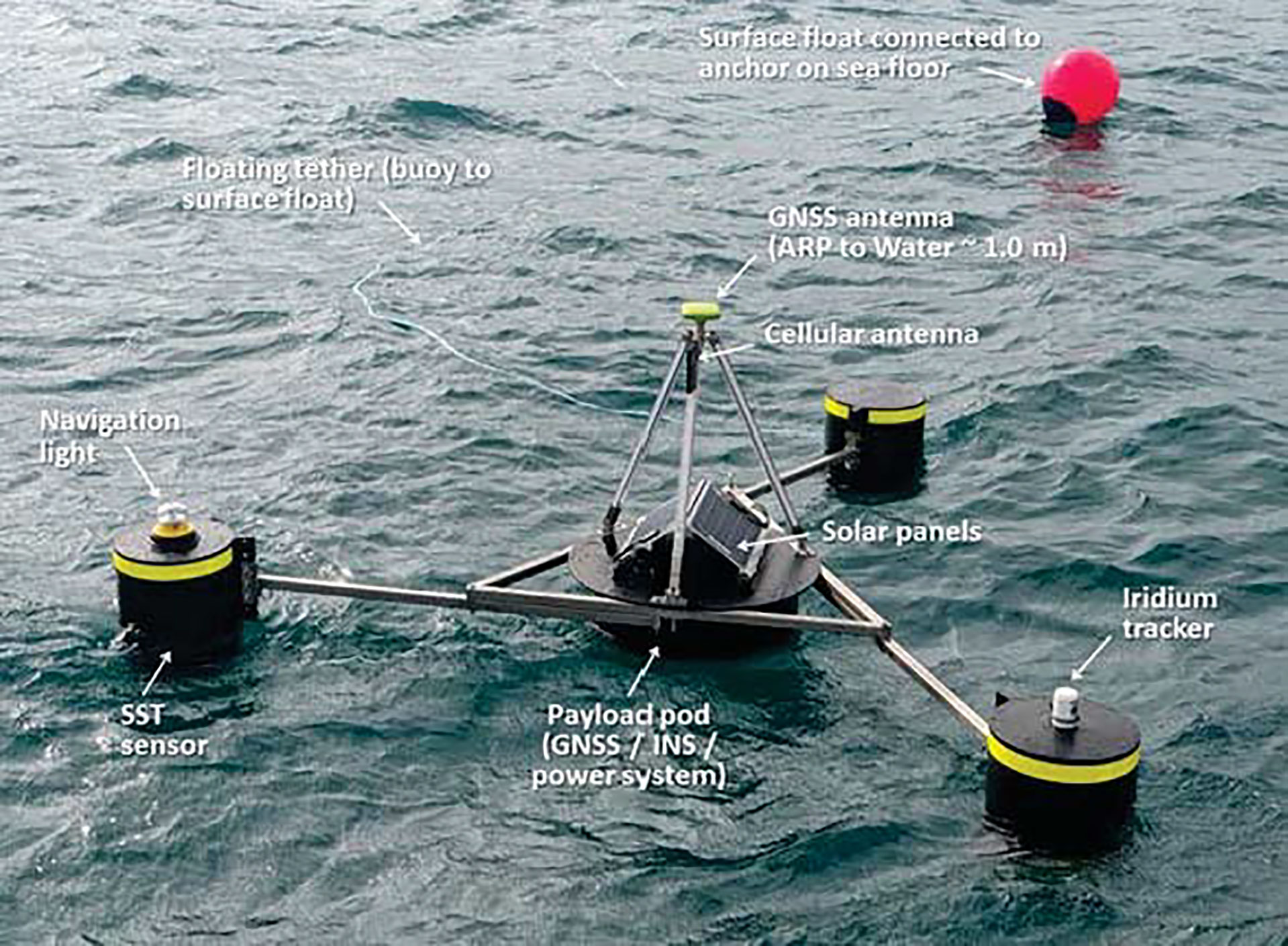
Figure 2 UTas/IMOS Mk-VI GNSS/INS equipped buoy with key features annotated in white text. Note the buoy is tethered horizontally from the upper float to the surface float which is in turn connected to the anchor on the sea floor. This enables the buoy to maintain position within a watch circle with a diameter of ~200 m in a water depth of ~50 m.

With the enhanced buoy design mentioned above, we develop the concept of a GNSS/INS equipped buoy array to offer flexibility for different validation configurations required for SWOT and future altimetry missions, as well as for other coastal applications. In our first trial development, the array is composed of 7 buoys along a S6MF track over a distance of 40 km. This enables us to explore the functionality of the array and help understand performance prior to further studies aimed at investigating the intra-swath variability for SWOT.

3.2 Moored oceanographic sensors

The in-situ mooring includes a bottom pressure recorder (BPR, SBE26+) at the depth of ~52 m along with a high-accuracy salinity and temperature sensor (SBE37) at ~25 m depth. A Nortek Aquadopp current-meter is installed at ~17-meter depth to measure the u (eastward) and v (northward) component of the current. All sensors are systematically calibrated in the laboratory to ensure they operate within the manufacturer specifications (Sea-Bird, 2021).

4 Data

4.1 In situ observations

The trial deployment of the buoy array we present here spanned 18^th to 26^th August 2021, yielding 193 hours (~8.0 days) of data from 6 Mk-VI buoys and 1 Mk-IV buoy (Figure 1). Global Positioning System (GPS) and GLObalnaya NAvigazionnaya Sputnikovaya Sistema (GLONASS) data are sampled at 2 Hz while the INS data is sampled at 100 Hz.

Data from the in-situ mooring include observations of current sampled at 20 min, and bottom pressure from the SBE26+ and temperature and salinity from the SBE37 at 5-min interval. Data from SBE26+ and SBE37 sensors are in turn used to derive the SSH (hereinafter referred as mooring SSH). The overhead barometric pressure at the mooring site is removed from the BPR series using pressure observed at the Burnie TG and the difference between JAS CP and Burnie extracted from the Australian Community Climate and Earth-System Simulator Global version Australian Parallel Suite 3 (ACCESS-G APS3) model (BoM, 2010). The corrected bottom pressure is then converted to SSH with a dynamic height correction computed from the temperature and salinity sensor (Watson et al., 2011).

4.2 Sentinel-6A NTC data

For this assessment, the standard high resolution Non-Time Critical (NTC) product from S6MF based on processing baseline of F06 is used. An overflight from pass 88 occurred over Bass Strait around 17:42:55 UTC on 25^th Aug. 2021. The majority of products used here are from both the 20-Hz (High-Rate) and 1-Hz (Low-Rate) archive, including radiometer observations, SWH and SLA. The data from the onboard High-Resolution Microwave Radiometer (HRMR, which is planned to provide access of decontaminated wet tropospheric correction closer to the coast (Donlon et al., 2021)) was not yet available at the time of this analysis. In Figure 1, both the low-resolution and the high-resolution waveform is shown to illustrate no obvious land contamination for the range observations at the corresponding buoy locations.

4.3 Other Observations and numerical models

Barometric pressure data from the nearby Burnie TG, along with hindcast sea level pressure fields extracted from the ACCESS-G APS3 model (BoM, 2010) is used to remove atmospheric pressure from bottom pressure measurements in order to derive the mooring SSH.

Wind stress at hourly interval from the ACCESS-G APS3 model is used to assess oceanic conditions during the deployment. The Finite Element Solution 2014b (FES2014b) tidal model (Carrère et al., 2015) is used for comparative analysis of estimated tidal constituents at five deployed locations. Additionally, the 6-hourly Dynamic Atmospheric Correction (DAC) product (LEGOS/CNRS/CLS, 1992) is used in the analysis of buoy SLA for comparison purposes.

5 Methods

5.1 Buoy and mooring data handling

Raw GNSS/INS data from 7 buoys are processed using double differencing method via our modified TRACK package version 1.31 (TRACK, 2011; Zhou et al., 2020). Details of processing setup are given in the supplementary material (Table S1). Outputs of interest from the processing are SSH and wet tropospheric delay. For outlier detection on the SSH series, any value larger than three times the standard deviation of the de-tided series is deemed an outlier and removed. Then any value larger than 1.5 times the interquartile range of the de-tided series over each 2.5-hour window is further removed as outlier. A 25-minute moving mean filter is applied to the processed SSH solutions to generate smoothed SSH series. An absolute gross error cut-off of ±0.06 m in range is further applied on the buoy minus mooring residual. A summary of the outlier removal process is given in Figure S2. SWH is calculated conventionally in hourly segments using four times the standard deviation of the detrended full-rate SSH data. Absolute wet tropospheric delay is extracted from output series for all 7 buoys.

We use the UTide Matlab package (Codiga, 2011) to undertake tidal analysis on both the mooring SSH and current-meter observations at the JAS CP. The merged decade-long mooring SSH series provides ample data to separate major tidal constituents and shallow water components. For computational efficiency, we restricted the two-dimensional (2-D) tidal current analysis to three years of input in length.

For the pure ocean tide component at deployment locations 10 km and 20 km either side of the JAS CP, the reconstruction is based on the tidal analysis of mooring SSH at the JAS CP plus an analysis of the differenced time series between the smoothed buoy SSH datasets from each location and the JAS CP. While these residual series are only ~8 days in duration, they are sufficient to separate constituents that we expect to show the greatest spatial variability (e.g., M2, M4, M6 and M8). We confirmed these were the likely dominant constituents in the tidal difference from JAS by undertaking a tidal analysis on the difference between mooring SSH at JAS and a previous secondary mooring-derived SSH at our Sentinel-3A comparison point (not shown here but near to our JAS+10 CP and 3 years in duration). It is worth noting M2 here represents the general semi-diurnal frequency term since we are unable to separate nearby constituents, such as M2 and N2, with series spanning just 8 days. We used tidal inference (Ray, 2017) on N2 (from M2) and P1 (from K1) using the built-in function in UTide toolbox to get a sense of the limitations in our tidal analysis – a full tidal constituent list from the mooring and residual tidal constituents from the buoys are provided in Table S2.

For comparative analyses of altimeter SSH/SLA, we derived buoy SLA for deployed locations using equation (1):

$\begin{array}{ll}\{ \begin{array}{c}SL{A}_{buoy}=SS{H}_{buoy}-Ocean Tide\\ Ocean Tide=Tid{e}_{mooring@JAS}+\Delta Tid{e}_{Buoy\to JAS}\end{array}& (1)\end{array}$

where Ocean Tide is based on results from tidal analysis of mooring SSH for the JAS CP location, whereas for other locations, a ΔTide with respect to JAS CP is also applied (as computed from the 8 days of buoy data).

5.2 Geostrophic current

Bass Strait is a relatively shallow sea (average depth ~60 meters) separating Tasmania from the Australian mainland. The mean width between Tasmania and the mainland is ~250 km, while the distance from east to west is ~500 km. The strait is typically relatively calm with an average SWH of ~1 meter. Bass Strait is dominated by tidal flow, with a dominant M2 constituent. The study site (Figure 1) is partially protected by island groups and the geometry of mainland Tasmania. These topographic features largely protect the study region from the major boundary currents (Ridgway and Condie, 2004; Ridgway, 2007; Baird and Ridgway, 2012), notably the South Australian Current from the eastern Great Australian Bight (GAB) to western Bass Strait and the East Australian Current on the eastern side. The location of the mainland Tasmania also provides some protection in terms of exposure to higher sea states from Westerly to South-Westerly winds that dominate the region.

Under the assumption of geostrophic balance, we investigated the observed versus inferred current from the sea surface gradient observed by the buoy array. The geostrophic current is calculated using the buoy array observed gradient based on equation (2):

$\begin{array}{ll}f·v=g·\frac{\partial h}{\partial x}& (2)\end{array}$

Where, f is the Coriolis parameter, v is the current velocity orthogonal to the defined x axis (along track), g is the local gravity constant and $\frac{\partial h}{\partial x}$ is the observed gradient between buoy pairs.

Given the goal in this paper is to provide primary assessment of the spatial scale of the noise in buoy SSH, comparison between the observed current and inferred current between buoy locations (based on the geostrophic balance assumption) is performed. We followed a three-step procedure: 1) first, the dominant tidal current observed is used to derive a possible azimuth bias of the orientation sensor in the current meter resulting in misalignment of the u/v components of the current meter with respect to the geographic east/north coordinate frame; 2) then, using the azimuth bias, the current observations are corrected; 3) finally, the tidal components are removed leaving the non-tidal current residual for comparison between the current meter and the buoy pairs. Further details regarding azimuth bias determination for the current meter can be found in supplement material (Text S1).

5.3 S6MF product comparison

As an illustrative example, 1-Hz and 20-Hz altimetry outputs including SSH/SLA, SWH and wet tropospheric delay from a single pass are assessed against derived quantities from the buoy array.

5.3.1 SSH by S6MF

We generate S6MF SSH by reinstating the high frequency atmospheric pressure fluctuation (DAC), ocean tide (FES2014b) and the mean sea surface (MSS), i.e., CNES-CLS15 (Schaeffer. et al., 2016) from standard S6MF output to the high-resolution SLA data:

$\begin{array}{ll}SS{H}_{alt}=SL{A}_{alt}+DAC+Ocean Tid{e}_{FES2014b}+MS{S}_{CNES-CLS15}& (3)\end{array}$

The above equation yields SSH from altimetry that is directly comparable with the filtered SSH data obtained from the GNSS buoy array – atmospheric and tidal signals remain in the observations. The bias between the altimeter and the buoy then becomes:

$\begin{array}{ll}Bia{s}_{SSH}=SS{H}_{alt}-SS{H}_{buoy}& (4)\end{array}$

We remind readers that given this comparison is from a single overflight, it is intended for illustrative purposes only. With that said, the comparison does give some insight into the shape of the sea surface, observed simultaneously by the GNSS buoy array and S6MF.

5.3.2 Wet tropospheric delay

Altimeter wet tropospheric delay is obtained from the low-rate S6MF product, given data from the HRMR onboard was not yet available by the time of this analysis. We extracted wet delay from the Advance Microwave Radiometer for Climate (AMR-C) measurements at 1 Hz along with the European Centre for Medium Range Weather Forecasts (ECMWF) modelled tropospheric delay (Fernandes et al., 2015; Fernandes and Lázaro, 2016) included in the product for comparison with values derived in situ from the buoy array.

6 Results

6.1 Precision assessment of Mk-VI buoy against Mk-IV buoy and in situ mooring

We first seek to understand the overarching precision of Mk-VI buoy used in our buoy array based on the knowledge of the prior Mk-IV design (Zhou et al., 2020). At the JAS CP, we have the triplet buoy group deployed in the vicinity of each other separated by approximately ~200 meters. Using the in-situ mooring as the “ground truth”, we probe the precision and the dynamics of the new design to assess any changes or differences with respect to the prior buoy design.

Figure 3 shows an inter-comparison of buoy-minus-mooring (B-M) residuals for all three buoys at the JAS CP. In the time domain, all three buoys show very similar patterns of difference against the mooring. The bulk of these common variations is likely to originate from high frequency atmospheric pressure variation, since the atmospheric pressure used to compute the mooring SSH is 3 hourly. The two new Mk-VI buoys show marginally reduced variability (root mean square of 1.8 cm and 1.9 cm for B11 and B08) compared to the Mk-IV buoy (root mean square 2.1 cm for B03). In the lower frequency bands shown in Figure 3B, the Mk-IV buoy tends to have marginally higher noise in the diurnal and semi-diurnal bands, while the two Mk-VI buoys show comparable performance with each other.

FIGURE 3

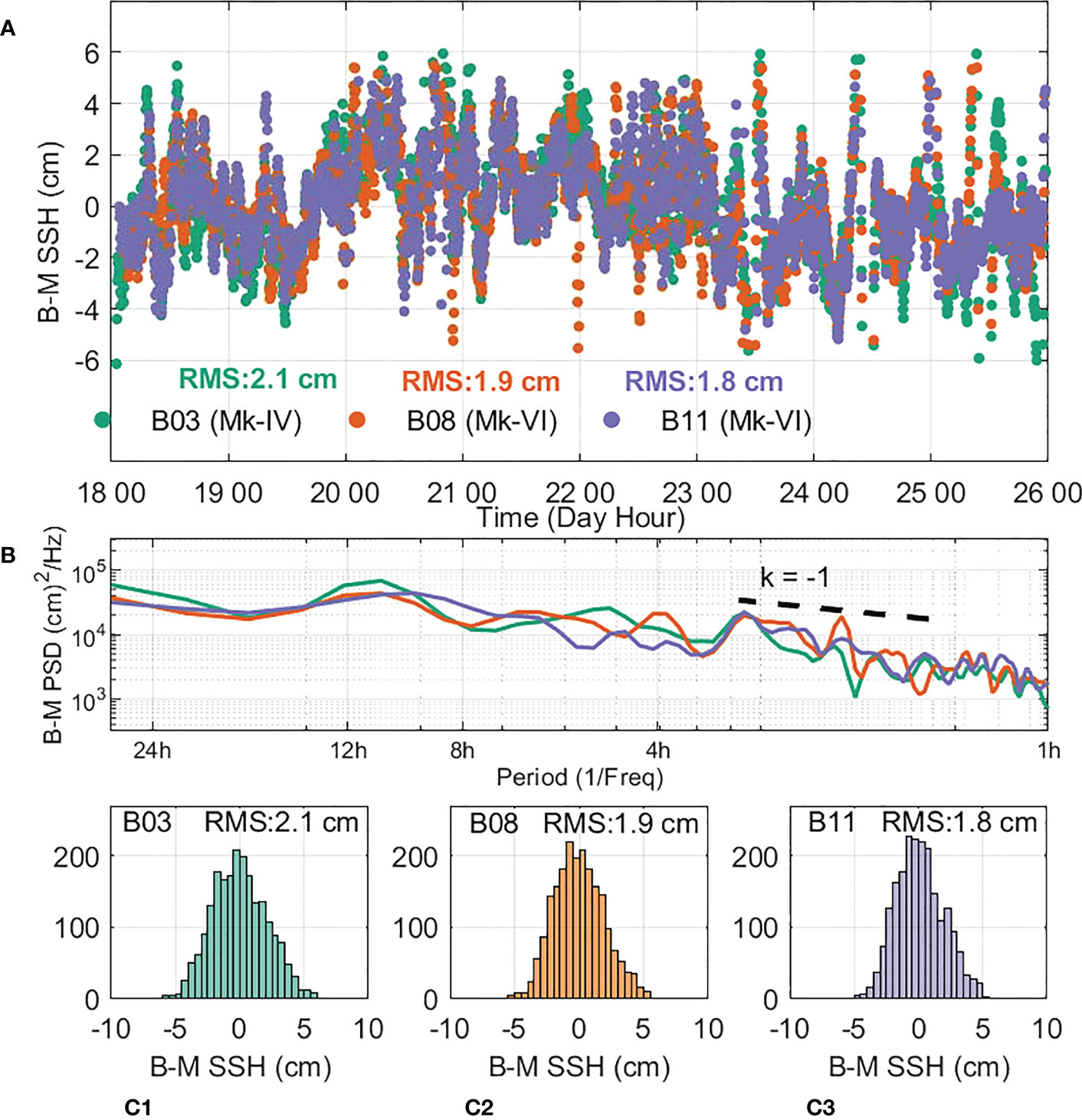
Figure 3 Inter-comparison of SSH solutions from Mk-IV, Mk-VIs and mooring. (A) shows the time series of B-M residuals for three buoys deployed at JAS CP, namely B03 of Mk-IV design, B08 and B11 of Mk-VI design. (B) shows the result of a power spectrum analysis on the BM residuals from three buoys. The dashed black line has a slope of -1, which presents a power spectrum of the flicker noise. (C1-C3) are the three histograms for the B-M residuals from three buoys. Colouring for the three buoys is consistent across all panels. Green for B03, orange for B08 and purple for B11.

On the other hand, differences against the mooring for all three buoys in the higher frequency bands exhibit a power law characteristic approximating flicker noise of similar amplitude (Figure 3B). These results confirm the new Mk-VI buoy design used in our array is of at least equivalent precision to the previous design, with improved performance over this ~8-day trial at the JAS CP. In the meantime, we also assessed the systematic noise baseline within the new Mk-VI buoy and between the new and the old (Mk-VI vs Mk-IV) buoys. By differencing SSH between buoy pairs from the triplet group, common GNSS error as well as some common oceanography are removed in the residual SSH series. Results show a similar noise baseline (~10 mm) compared to the quantity previously reported (~8.5 mm) derived from historic twin deployments by Zhou et al. (2020) (see Figure S3). We note the buoy triplet reported here has larger separation between buoy pairs compared to those investigated previously (200 m versus 50 m), and this is the likely source of the small increase in statistics.

As a sanity check, we also compared the dynamics of Mk-IV and Mk-VI design under the same impact of external forcings – selecting B03 (Mk-IV) and B08 (Mk-VI) from the triplet group. Results in Figures S4 and S5 show similar response to the forcings as evidenced in GNSS and/or INS derived accelerations and GNSS derived wave directions. This indicates the dynamics of the buoy platform has not changed dramatically during the design transition.

6.2 Differences in tide and sea states along-track from the buoy array

The buoy array deployed with 10-km spacing over a distance of 40 km enables the characterisation of differences in oceanic conditions extending from near-shore (JAS-20, ~16 km from the coast), to offshore (JAS+20, ~40 km from the coast). Here we focus on differences in tide and sea state.

Figure 4A shows observed tidal differences relative to the JAS CP. Either side of the JAS CP, the tidal differences reach ±0.05 m, increasing to ±0.1 m for sites 20 km either side. A spectrum analysis of these series (Figure 4B) indicates that the majority of the difference is in the semi-diurnal band, while there are some localized variations to the shallow water components, mostly residing in M4, S6 and M8. Within the dominant semi-diurnal band from sites 20 km either side of JAS, the amplitude of the differences is up to 0.05 m, and as expected, approximately half of that for sites 10 km either side. For all other shallow water components, the differences in amplitude are ~0.01 m or less.

FIGURE 4

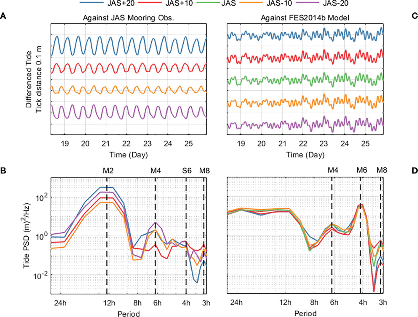
Figure 4 Tidal difference along track by five buoys based on mooring SSH and the FES2014b Model. (A) shows the tidal difference of the harmonic predictions at each location differenced against the prediction at JAS which is based on the mooring SSH; (B) present the power spectra analysis of tide differences against JAS CP, with the four dashed lines indicating different tidal constituents, namely M2, M4, S6 and M8; (C) shows the tidal difference from each buoy against FES2014b at each deployed location – standard deviation of the differenced series calculated to be 2.7 cm; (D) shows power spectra of tide difference between extraction from model and from observations at five locations, with dashed black lines at M4, M6 and M8. (A, C) have lines offset by 0.2 m for clarity. Colouring across all panels consistently follows the legend at the top. All tides are sampled and reconstructed at 1-min interval.

We also performed a comparison between the FES2014b ocean tide model and our buoy derived ocean tide (panels on the right side of Figure 4). For all buoys at the five locations, the absolute difference between the buoy derived tide and the model is up to ~ ± 0.07 m, with its upper quartile located at just ~0.01 m and standard deviation at 0.027 m. The spectrum in Figure 4D indicates the shallow water terms are the major source of difference between the model and our extraction based on observations (dominated by differences at M4, M6 and M8). As for the amplitude difference of these shallow water constituents between model reference and buoy observation (provided in Table S3), M6 has the most significant difference of ~0.02 m, while all others are at sub 0.001 m level. This difference for shallow water tidal components between buoy and FES2014b emphasises the possible role of buoy array observations in initial SWOT validation. We will elucidate this further in discussion.

We use SWH as a metric to define sea state. Figure 5 shows the SWH time series derived from the buoy SSH series over the full deployment computed in hourly bins. There is clear evidence of a small but significant gradient in mean SWH along the array (~1.0 m nearest to shore at JAS-20 and ~1.2 m furthest offshore at JAS+20). The increased exposure at greater distances from the coast (see Figure 5A) is evident throughout the deployment.

FIGURE 5

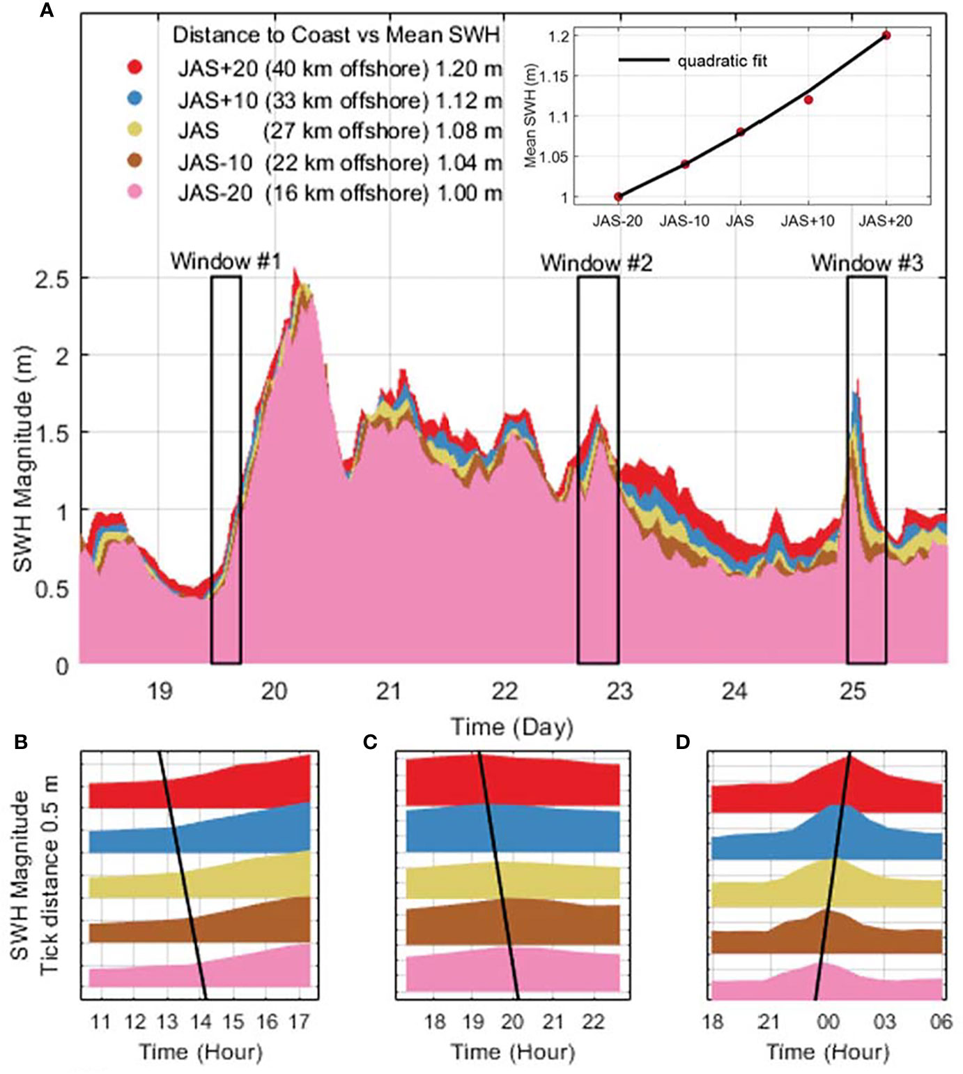
Figure 5 Sea states along track quantified by buoy SWH at five locations. (A) shows SWH over the full span of the deployment. Mean SWH statistics are included on the figure, as well as the distance to shore from five deployed locations for the buoys. The three lower panels (B–D) are example cases used to investigate the energy propagation along the buoy array. The three time periods correspond to the black inset boxes in (A). Black solid lines in lower panels are qualitative and signify times of comparable SWH corresponding to the passage of frontal systems in the area.

In the time domain across all five locations, there is clear evidence of the passage of weather systems leading to differences in the time of onset and dissipation of energy. In three selected time windows, a transition in sea state is observed (see black boxes, Figure 5A). The first case (Figure 5B) sees a difference of ~1 hour in the arrival time of the wind event causing SWH to increase by ~100% from 0.5 m to 1 m. In the second case (Figure 5C), we observe the recession of an event which takes ~1 hour to reach the near shore site at JAS-20. In the last case (Figure 5D), we see the onset of a south-easterly system (evidenced by online historical climate data from Bureau of Meteorology) affecting the inshore site first, reaching JAS+20 in ~1 hour.

6.3 Wet tropospheric delay along buoy array

Similarly to SWH, we characterise the spatio-temporal evolution in tropospheric delay estimation from the GNSS buoy array (Figure 6). In the time domain, we observe approximately consistent tropospheric delay from the buoys at five locations. The buoy array does, however, capture some regional changes in the distribution of water vapour. This is evident in Figure 6C, where we are likely observing a frontal system moving eastward, as observed by buoys at three locations further away from shore – JAS, JAS+10 and JAS+20. Additionally, as with SWH, in the spatial domain we can also clearly identify the passage of events that are associated with the passage of water vapour in the atmosphere. For example, in the same temporal period as identified in Figure 5D, we see the passage of an atypical ~south-east to ~north-west event. It indicates that each buoy observed an increase water vapour content, taking ~3 hours to extend from the nearshore to the offshore location.

FIGURE 6

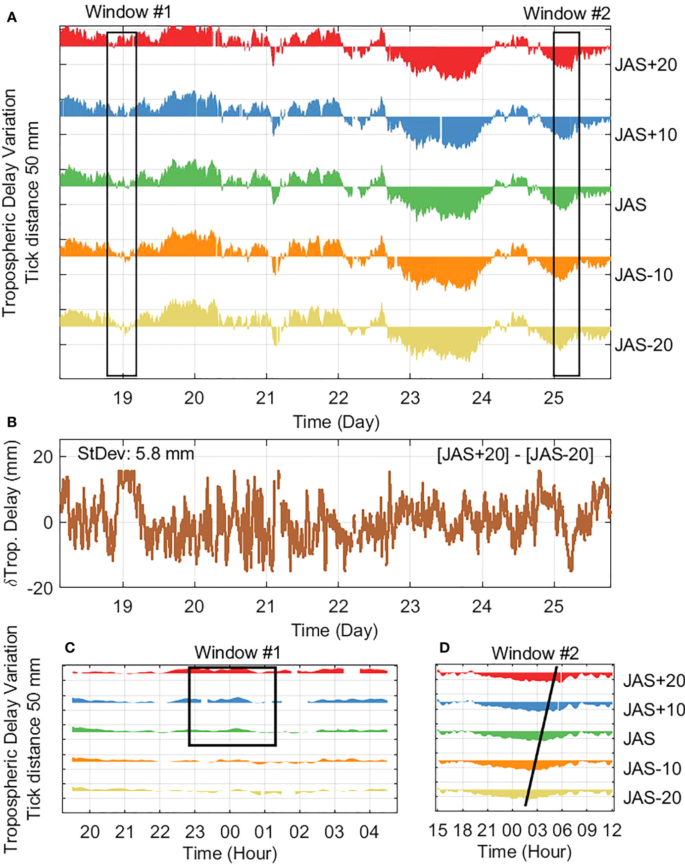
Figure 6 Wet Troposphere Delay observed by buoy array. (A) shows the tropospheric delay estimation by buoys at five locations. All five series are referenced against the same median value, hence shows the relative variation along the time axis across the buoy array. Black rectangles are for selected weather windows. In (B), the difference between tropospheric estimations at JAS+20 and JAS-20 location is shown along with the range and the calculated standard deviation. (C) shows a case where regional front system affects part of the buoy array. (D) show a case of front progression over a duration of 3 hours aligned with the same window in Figure 5D, with the black line indicating the approximate arrival time of the increased water vapour associated with the passage of a south-easterly frontal system.

When comparing the JAS+20 to JAS-20 CP over a distance of 40 km (Figure 6B), we observe a range over ~20 mm, with a standard deviation of 5.8 mm. As the distance decreases to 20 km and further to 10 km, the range and the standard deviation continues to drop as expected. The variability of the differenced tropospheric delay has a range of ~10mm over a distance of 20 km, while the standard deviation is at a level of ~3 and ~4 mm over a distance of 10 and 20 km respectively (provided in Figure S6). This gives an important first sense of the variability expected over ~50 km, approximately consistent with the width of a SWOT-swath. We return to this point in the discussion.

6.4 SLA from the buoy array

In previous sections, we evaluated the performance of the Mk-VI buoy with respect to its predecessor and then characterised the spatial and temporal variability in tides, SWH and troposphere using the buoy array. We now seek to evaluate the residual SLA along the array – see Eq. (1) for SLA determination.

In Figure 7, SLA series derived from the buoys at each location are shown, all expressing a semi-diurnal signal with variable amplitude (reaching a maximum magnitude of ~150 mm) over the duration of the deployment. The apparent semi-diurnal signal appears to be amplified commencing approximately on day 20 corresponding to an increase in wind stress (see blue line, Figure 7). This exacerbation gradually decreases over the following 2 days (see shaded window, Figure 7). The phenomenon shown is likely a perturbation to the M2 tidal resonance in Bass Strait driven by meteorological forcing as previously reported by Wijeratne et al. (2012). The DAC series from a 6-hourly numerical model is shown over the SLA series (Figure 7), showing some correlation yet a noticeable phase delay and inadequate temporal resolution.

FIGURE 7

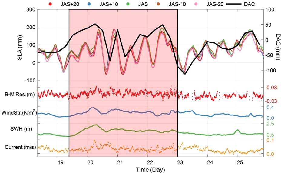
Figure 7 SLA from buoy array. The upper half of the figure shows the SLA series group (coloured thin lines) from the buoy array aligned with the DAC series (solid black line). The lower half of the figure includes 20-min non-tidal current, 1-hourly SWH, modelled hourly wind stress (WindStr.) and the 5-min B-M residuals. (B-M Res.) The shaded black rectangle box highlights a selected duration of interest, where a ~12-hour signal was observed within the time span in the SLA series.

Quantities in the lower part of Figure 7 show that on the second day of the deployment, the wind (inferred by observed SWH and modelled wind stress) increased. Following that, a resultant rise in the velocity of the non-tidal current was observed. To further investigate the time variable resonance observed during the deployment of the buoy array, we plotted one-month of mooring SSH at the JAS CP and contemporaneous wind observed at the Burnie TG (see Figure S7). The excitation of the resonance shows clear relationship with the windspeed, and we return to this in the discussion.

6.5 Buoy precision assessed from the perspective of the geostrophic current

Based on our along-track SLA profile from 7 buoys, the computation of the inferred geostrophic current between successive pairs of buoys, and comparison to the observed non-tidal current provides some insight into the spatial scale of the systematic errors in the buoy SSH solutions. Here we recursively formed buoy pairs of a certain separation distance, and then following the assumption of geostrophic balance, we derived the inferred geostrophic current between the buoy pair using the sea surface gradient computed from SLA differences. Derived current series were then organized into five groups based on the separation: <1 km, 10 km, 20 km, 30 km and 40 km. We used Welch’s method (Welch, 1967) to estimate the power distribution in the frequency domain and stack the results to obtain the median spectrum for each group other than the <1 km group due to its low Signal-to-Noise Ratio (SNR) as evidenced in Figure 8F. For each pair-wise geostrophic current series, we computed the standard deviation and investigate this as a function of buoy separation distance. Inferred current centred at the JAS location from buoy pairs were then compared directly with those observed from the in-situ current-meter (Figures 8B, C, E)

FIGURE 8

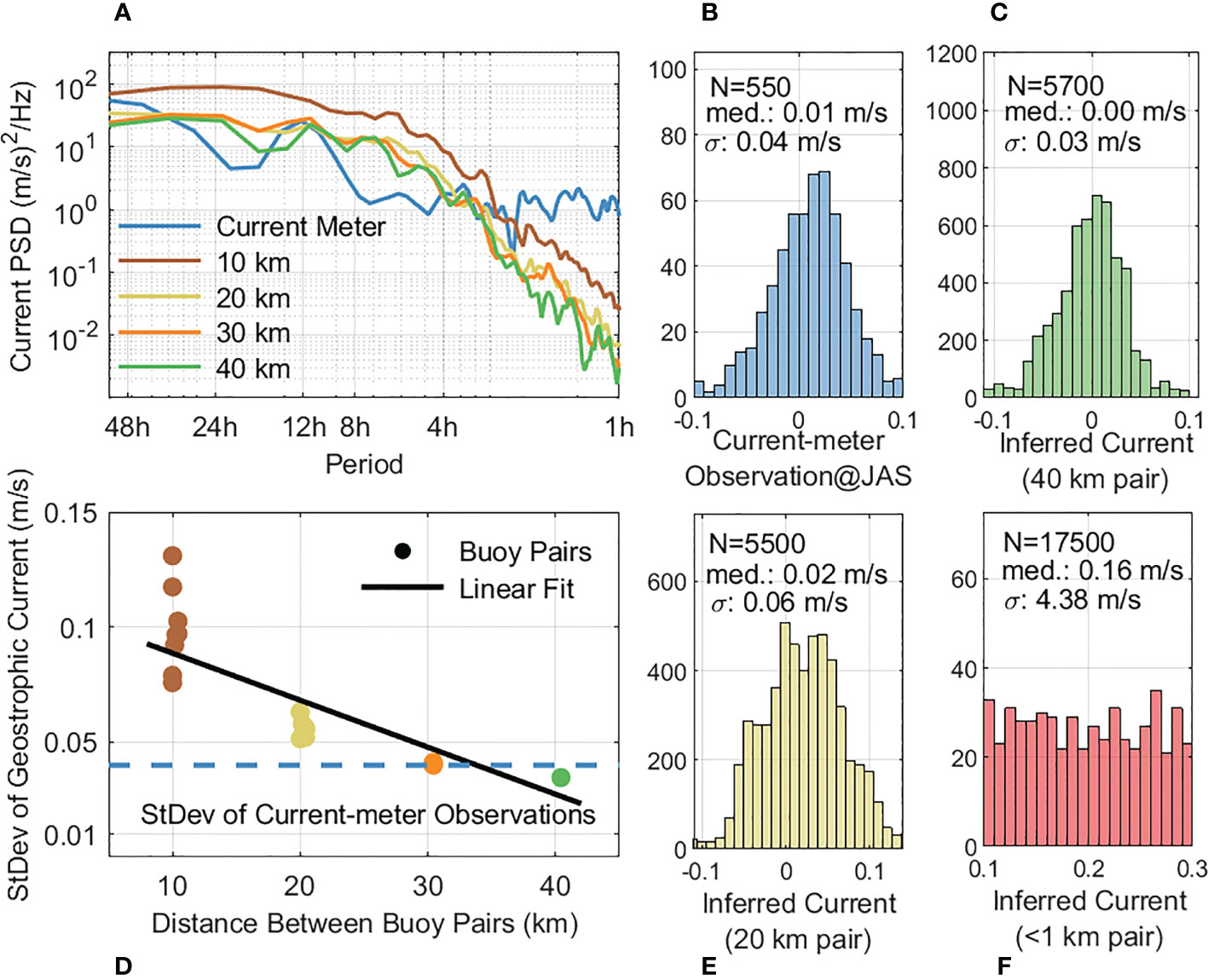
Figure 8 Non-tidal geostrophic current statistics inferred from sea surface slope between buoy pairs. (A) shows the median spectrums for current series from different buoy distance pair groups and the current meter. (D) shows the best line of fit between standard deviation of the derived current series and buoy pair distance, the blue dash line shows the standard deviation of the point-based observations inferred from the current-meter at JAS. The four histograms on the right – (B, C, E, F), are from the current-meter and the buoys pairs at different distances yet centred at the JAS CP. Colouring across the panels follows the pattern in (A). N indicates the sample size for each histogram, σ presents the standard deviation, and med. is short for median.

In Figure 8A, the spectra show that the highest level of energy (in the form of magnitude of variance) is found in buoy pairs with ~10 km separation, with some coloured noise evident at periods shorter than about 8 h. As the buoy separation increases, the energy level in the inferred current series decreases yet the coloured noise structure is maintained. As expected, the buoy pair with ~40 km separation has the least magnitude of variance among the four groups. The spectrum computed from the non-tidal observations of the current meter shows largely white noise as inferred from the slope of the spectrum over bands below 8 h. An obvious reduced level of energy can be seen between 8-h and 4-h period bands in the current meter when compared with buoy pair spectra. We return to this in the discussion.

The standard deviation of the inferred current time series from buoy pairs at different distances follows a negative quasi-linear trend with the buoy distance from ~0.1 m/s at 10 km to ~0.03 m/s at 40 km (Figure 8D). In comparison, the standard deviation of the observations from the single current-meter is ~0.04 m/s (Figure 8B), which is at comparable magnitude to that of buoy pairs over 20 km and 40 km (Figures 8E and 8C respectively).

6.6 Buoy precision assessed from the perspective of the S6MF products

By way of an example, we now compare the buoy array data against the concurrent overpass of S6MF high resolution data (both 1 Hz and 20 Hz). Commencing with the wet delay, Figure 9A shows the delay from the S6MF radiometer, the ECMWF model and as observed at each buoy location. We see an increasing trend with distance along track (i.e. increasing further offshore) in all three series. However, for the radiometer observations, some additional spatial variability along track can be observed, especially within 10 km either side of JAS – from J-10 to J+10 (Figure 9A). The three buoys located close to the JAS CP in Figure 9A gives some indication of the intrinsic precision of estimated wet tropospheric delay from the buoy array (~3 mm in this case).

FIGURE 9

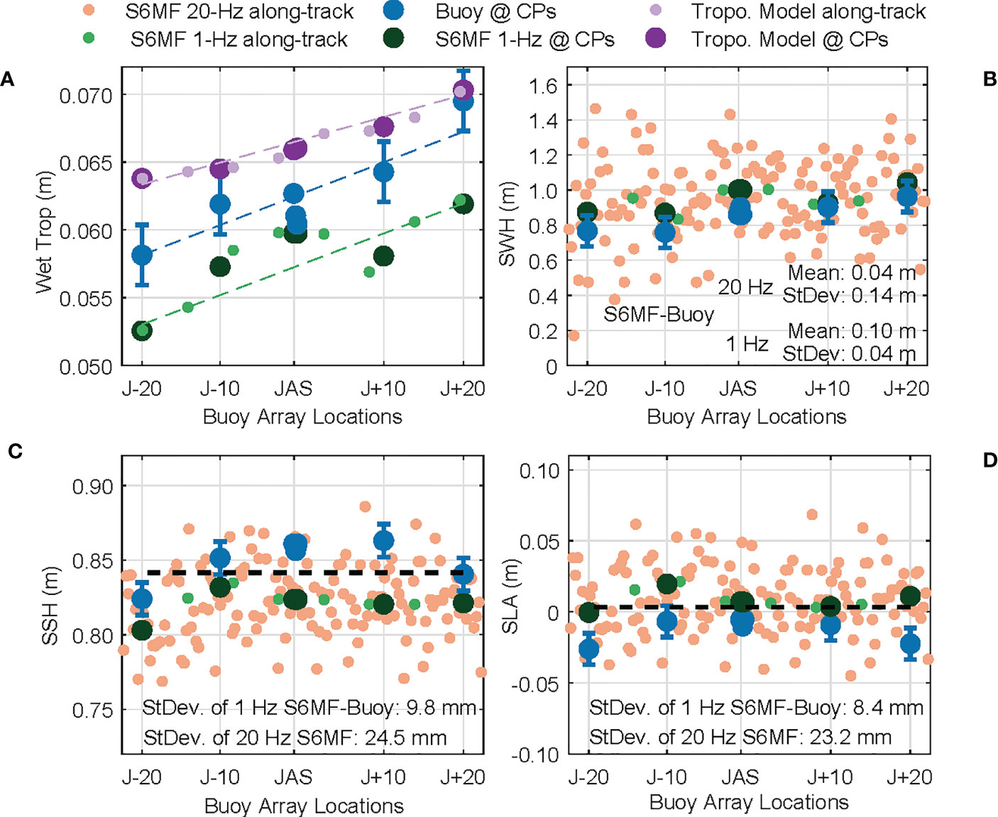
Figure 9 Comparison between high-resolution products of S6MF and observations from the buoy array. (A) shows the observed wet tropospheric delay from buoy and the radiometer onboard S6MF and a numerical model. Fitted lines show linear fits between locations and wet tropospheric delays; (B) shows the along-track 1-Hz and 20-Hz SWH quantities derived by both the altimeter and the buoy array. (C, D) show SSH and SLA respectively. Dashed black lines shows the median of the SSH or SLA outputs by S6MF over the buoy array. In all panels, large dots refer to specific quantity at the buoy array locations. Smaller dots are 20-Hz or 1-Hz S6MF data along track. The error bars shown on buoy data are indicative of intrinsic precision as determined from the triplet buoy group at JAS CP in each case.

In Figure 9B, the 20-Hz SWH derived from the slope of the leading edge of the altimeter waveform has a standard deviation of 0.14 m along the buoy array with a mean difference of 0.04 m against the buoy derived SWH. The SWH from the buoy array shows a quasi-linear trend with increasing distance along track (i.e. increasing further offshore). A similar but far more uncertain trend is evident in the 20-Hz SWH altimeter series. We also note the 20-Hz SWH appears more variable closer to the shore (around J-20 and J-10). Meanwhile, 1-Hz SWH from S6MF appears to be more consistent with the trend of buoy SWH in Figure 9B – standard deviation of the difference being merely 0.04 m, although it is ~0.10 m larger on average than the conditions sensed by the buoy. Moreover, a consistent low frequency signal is observed in both 1-Hz SWH from S6MF and from the buoy array, highlighting a likely finer scale signal in the spatial variability of SWH.

SSH measured by both S6MF and buoys shows consistent behaviour along track (Figure 9C). When differencing S6MF(1 Hz) SSH solutions against those from the buoy array, the standard deviation is only 9.8 mm. It is reduced to 8.4 mm (Figure 9D) when comparing SLA solutions. The curvature in the S6MF data (along track) appears to be flatter than that of the buoy derived SLA series, especially at JAS+20 comparison point – furthest from shore. We will return to this in the discussion.

7 Discussion

The development of the buoy array concept is an important progression in the use of GNSS/INS equipped buoys for the validation of next generation satellite altimeters – and for other possible applications in the marine domain. Such an array offers the simultaneous observation of sea surface height in a geocentric reference frame, significant wave height and wet troposphere delay at high temporal resolution. While the spatial resolution is simply limited by the number of buoys, the precision of the approach requires detailed investigation in order to optimise future deployment.

7.1 Precision assessment of the buoy array

Historically, SSH solutions based on GPS from the Mk-IV buoys have provided a significant contribution to altimetry validation at the Bass Strait facility. Based on this design, we have further enhanced processing through the integration of INS and improved handling of GNSS (Zhou et al., 2020). In order to realise the buoy array concept and prepare for SWOT validation, remote telemetry and sustained operation in higher sea states are key requirements. To achieve this, the Mk-IV design was effectively scaled up, adding a solar power system and cellular/iridium communication. We present results from a trial deployment over ~8 days as an initial proof of concept. All buoys maintained anchor location, functional voltage (> 13 V), tracking quality and communication in SWH up to 2.4 m.

Interpretation of the precision of the buoy approach against the in situ mooring SSH requires consideration of the systematic errors affecting the moored oceanographic sensors. The removal of atmospheric pressure from the integrated pressure observed by the bottom pressure gauge is one key error source (noting it is derived from 3-hourly observed pressure at the Burnie TG with a correction to the JAS CP based on data from the ACCESS meteorological model at hourly interval). Such a series is unlikely to adequately reflect high frequency changes in atmospheric pressure. Errors in the dynamic height correction inferred from temperature and salinity observations are also likely but difficult to quantify. Given the column is generally well mixed, we expect these errors to be quite small, especially over the 8-day period investigated here. For now, we aim to get a general sense of the upper bound of the SSH errors within our validation system and note that errors in the mooring SSH are also a contributing factor to the B-M residuals presented.

Results in Figure 3 confirm that the new buoys are working at equivalent precision to their predecessor whose performance has been systematically assessed in previous studies in Bass Strait (Zhou et al., 2020). Comparison of the new buoy against the in situ mooring shows marginally smaller root mean square (RMS) differences (~0.1 cm) compared to the previous design, possibly due to the incorporation of the INS. Nevertheless, it is challenging to determine the significance of this result given this trial deployment of the buoy array was for just 8 days. More twin/triplet-buoy deployments would be required to gather more evidence of an overall improvement in the precision of the Mk-VI buoy.

Some further evidence of improvement can be observed in the spectrum in Figure 3, where a reduced level of energy is seen at both the diurnal and semi-diurnal frequency bands for the new design. The increased size and weight of the Mk-VI design (and thus greater moment of inertia), along with an increased antenna height may be the source of these improvements. Although quantities derived to describe the buoy dynamics in Figures S4 and S5 suggest no dramatic changes were evident during the transition of the design, a lack of INS observations on the old design during this deployment prevents us from further probing the relatively changes to dynamic behaviour (e.g. comparison of angular-rate and pitch/roll/yaw observations, etc).

For both buoy designs, we see a consistent coloured noise pattern observed in the <8 hour period bands – this likely reflects systematic error contributions from the GNSS solutions (Geng et al., 2018), as well as possible contribution from high frequency changes to atmospheric pressure affecting the mooring. We see no evidence of significant semi-diurnal signals in the B-M residual that were observed for the old buoy under specific conditions (up to 2 cm with 1.15 m of mean SWH as presented by Zhou et al. (2020)). This may reflect improvements to the tether system, yet more data is required over a broader range of conditions (sea state, wind, current etc) to assess this more comprehensively.

7.2 Oceanic characteristics observed by buoy array

7.2.1 Tidal difference along buoy array

Over the 40-km distance along the buoy array, tide profiles were expected to vary given the shallow bathymetry and proximity to the coast. In Figure 4A, absolute tidal height differences reach 0.2 m across five locations due to the sum of variations in amplitude and phase across various frequency bands (mainly M2 and inferred N2) from the buoy array observations. The marginal difference of the energy level at the semi-diurnal band of the spectra in Figure 4D, suggests that the FES2014b model with a spatial resolution of 1/16° represents the spatial propagation of semi-diurnal signals quite well.

It is expected that in a shallow shelf environment such as Bass Strait, the tide observed with the buoy array would show some notable differences to a contemporary assimilated tidal model (FES2014b in this study). The most significant difference emerges in the higher frequency shallow water constituent M6 which is up to centimetre level. This is expected, since M6 is a non-linear wave which would likely include a time variable amplitude component driven by atmospheric forcing (Friedrichs and Madsen, 1992; Cook et al., 2019) (unable to be captured by the tide model). This further indicates the complexity of tide characteristics in a shallow strait such as Bass Strait (Wijeratne et al., 2012). Despite the outstanding quality of the global tide models, the buoy array deployed in this coastal shallow sea location highlights some space for improvement in the tide model; this reiterates the challenge that the tidal issue presents in the lead up to interpreting swath altimetry data.

7.2.2 Sea States along the buoy array

From inshore (JAS-20) towards offshore (JAS+20) deployment locations, there is increased exposure to the prevailing weather dictating increased average sea state. This increase in sea state is observed clearly along the buoy array in Figure 5A. Given its geographic location and partial protection by large islands on the western and eastern boundary, Bass Strait is partially isolated from highly energetic ocean processes (Liu et al., 2022). This unique feature dictates relatively calm sea states in the region of the validation facility, with a mean SWH at the JAS CP of ~1 m. The spatial and temporal variation in SWH (up to 2.5 m) is highlighted with the results from the buoy array over the ~8-day trial deployment.

A further finding from Figure 5 is the ability of the buoy array to monitor the temporal and spatial evolution during the propagation of a specific meteorological or oceanographic event. The likely explanation for the transition in SWH magnitude within the first two selected time windows (see Figure 5A, Window #1 and #2) would be the passage of frontal systems in the typical west to east direction. As the system moved across the array, the increased sea state (quantified by SWH magnitude) followed closely. The third case suggests a featured case where a south-easterly wind is driving the increasing sea state further offshore – usually linked to winds that follow the passage of low-pressure frontal systems in this region. Over the selected windows shown in Figure 5, the propagation speed is typically 30-40 km/hour over this trial deployment. While the propagation provides interesting insight into the dynamics of air/sea interaction in this part of Bass Strait, it is the spatial variability that is of greatest relevance to the future interpretation of data from swath-based altimetry. The concurrent deployment of wave Acoustic Doppler Current Profiler (ADCP) in conjunction with the buoys in future deployments should further assist to illustrate the wave field propagation more comprehensively.

7.2.3 Tropospheric delay along the buoy array

The integrated wet tropospheric delay above the antenna is a well-known valuable by-product of GNSS processing (Jones et al., 2020; Li et al., 2020). With the formation of a buoy array, the spatial and temporal variability associated with the passage of weather systems can be clearly observed. In Figure 6, such an event can be seen towards the end of the buoy deployment (Figure 6D). Over a course of 3 hours, we observe the transition in the water vapour signal in the direction from the inshore to offshore, possibly driven by the same system that similarly impacted the sea state (specifically during the third showcase period in Figure 5). This again highlights the value of the buoy array to characterise both the spatial and temporal variation of atmosphere path delay, which is one key factor to consider for the future swath-based altimetry mission to decorrelate and in turn resolve (sub-)meso-scale ocean process. In a broader context, it highlights the potential value to other application areas, extending the value of land based GNSS sites for meteorological studies into the marine domain (Ahn et al., 2005; Williams and Nievinski, 2017; Singh et al., 2019).

Noting that SWOT will use a single radiometer to observe the wet tropospheric delay over an entire 50 km swath, further investigation of the spatial variability in the observed delay from the buoy array is warranted. The difference between delay estimated by buoys separated by 40 km has a standard deviation of ~5.8 mm. It should be noted that the tropospheric water content above any given buoy is estimated from available GNSS observations along slant ray paths and mapped to the zenith. GNSS derived zenith delays are therefore spatially averaged to some extent (with the spatial resolution dependent on various GNSS related settings such as elevation cut off, as well as dependent on the vertical distribution of water content in the atmosphere). In this study, as shown in Figure 6B, a number of clear signals can be observed within the differenced series. The radiometer on board SWOT or the ECMWF troposphere fields are insufficient either in spatial or temporal resolution to capture these higher order effects. From the design requirements, SWOT has a residual wet troposphere delay threshold of 4.3 mm over 15-1000 km after cross-track radiometer correction (Esteban-Fernandez et al., 2017). The combination of high resolution regional atmospheric modelling [e.g. ACCESS (BoM, 2010)] and wet delays from our land and ocean based GNSS instruments offers the potential to validate this threshold and assess its impact on the interpretation of ocean dynamics. Yet, careful analysis will be required to assess the spatial scale at which the GNSS buoy array can derive independent estimates of wet delay, and work to investigate this remains ongoing.

7.3 SLA and geostrophic current by the buoy array

7.3.1 SLA and surface forcings

Dynamic changes in ocean state (temperature, salinity, pressure) are all expressed in SLAs derived from satellite altimetry. The effects of ocean tides and the atmosphere are typically removed in the formation of the SLA, leaving the dominant effects of circulation and changes in ocean properties. The challenge, particularly in shelf sea settings such as Bass Strait is the accuracy of tidal and dynamic atmospheric corrections. Indeed, our 8-day trial deployment of the buoy array exposes this issue well having observed an excitation of the tidal resonance in Bass Strait, likely induced by wind forcing (see the shaded region pertaining to the excited semi-diurnal signal, Figure 7). This period corresponds with the passage of a frontal system (confirmed by the ACCESS-G wind stress and GNSS buoy SWH time series). The resonance phenomena in Bass Strait was investigated by Wijeratne et al. (2012). Such an effect occurs regularly in Bass Strait, where changes to wind forcing is thought to cause a nodal shift of the tidal resonance at M2. Additional data over one month plotted with observed wind speed from the Burnie TG confirms this (see Figure S7). Similar cases are observed in other similar basins (Garrett, 1972; Lin et al., 2001; Burling et al., 2003; Arbic et al., 2007).

Analysis of the DAC supports our findings and reinforces the limitations of the modelled corrections used to generate SLA in this region. The DAC (black line, Figure 7) shows a clear correlation with the SLA. However, small but clear phase differences are observed between the in-situ SLA and modelled DAC. We attribute this to the DAC model having insufficient temporal resolution of just 6 hours. The atmospheric model used in the DAC also lacks the precise timing of the onset of this frontal system compared with the in situ observations. This presents clear challenges to the oceanographic interpretation of conventional SLA data that includes a modelled DAC correction and highlights that buoy array observations will be useful to assess enhancements to DAC models currently under development.

7.3.2 Geostrophic current derived from the buoy array

Understanding the impact of the errors in the buoy SSH in the spatial domain is critical. This dataset provides an early opportunity to explore the attainable scales of oceanic signals in Bass Strait for given configurations of the array. For this goal, we performed an analysis of the inferred geostrophic current determined from buoy pairs and compared these against the current-meter observations at the JAS CP.

This analysis is based on certain assumptions. The broad area where the buoy array is deployed is assumed to be in geostrophic balance and the geographic variability of the current to be small – a broader assumption is that barotropic rather than baroclinic conditions dominate Bass Strait. Given the water depth is at ~50 m, most ocean signals expected are assumed to be at the several 100-m spatial scale and operating over time scales of hourly up to daily. With these assumptions, we exclude most of the possible higher-order ocean processes that might disrupt water flow (including the effects of bottom friction noting the current meter was deployed at a depth of ~17 m where total water depth was ~52 m). This in turn leads to a first pass assessment of the spatial error scales associated with water surface elevation determination via the buoy approach without confounding contributions from the small-scale ocean-atmosphere interactions.

As mentioned in the “method” section, tidal geostrophic current is used in this paper to estimate azimuth bias of the current meter, while the non-tidal residual is assessed for the spatial scale of the errors in buoy SSH. This decision is made on the grounds of the following: 1) Bass Strait is dominated by the semidiurnal lunar M2 constituent (McIntosh and Bennett, 1984; Wijeratne et al., 2012); 2) azimuth bias of the current meter is better estimated with a high SNR oceanic signal; 3) with Bass Strait being a rather benign field sheltered from major current boundaries (Ridgway, 2007; Baird and Ridgway, 2012), the non-tidal residual from either current meter and the buoy system is expected to be composed of mainly the contribution from the systematic errors rather than oceanic processes. For those interested, the tidal current statistics are provided in Figure S8 – we focus here on the analysis of the non-tidal current.

It can be inferred from the spectrum in Figure 8A that the uncertainty of the current inferred from the buoy-pairs decreases significantly as the distance between the buoys increases from 10 to 20 km. This is due to the noise from buoy SSH having a greater contribution to the computed sea surface gradient over shorter distances. As the buoy pair separation increases, so does the signal to noise ratio. When compared with the buoy spectra, the reduced variance in the current meter series between the 4-8-hour band suggests that the current observed by the current meter underwater is slower than those inferred from the buoy based on the surface height gradient. This points to the possible limitations of overarching assumptions involved in this comparison, in particular, the interpretation of the current at ~17 m depth and the assumed spatial scale of the variability. Again, the development and concurrent deployment of shallow water current, wave, pressure inverted echo sounder (CWPIES) is underway to address this.

In Figure 8D, a reducing trend in the standard deviation can be observed as the spacing between buoys decreases. The magnitude of standard deviation between the buoy pairs and current meter starts to become equivalent at 20 km spacing which provides vital information for future SWOT validation activities. Conversely, it should be noted that the standard deviation of the non-tidal geostrophic currents in Figure 8D inevitably includes the contribution from fine scale oceanic signals (e.g., coastal jets, high frequency atmospheric pressure turbulence). This highlights that the spatial scale of the noise in the buoy solutions needs to be well understood in order to interpret swath observations from SWOT.

The histograms in Figure 8 indicate two findings. First, the high level of variation between the buoy-pairs at JAS (< 1 km separation) makes interpretation of the inferred current over such short distances non-sensical – noise very likely being dominant even when considering possible flaws of the underlying assumptions. Second, current inferred between buoy pairs over 20 and 40 km distance is of similar variability to that of the observed current. Medians of the current from these buoy pairs and the current meter remain insignificantly different from zero, verifying that the deployment area in Bass Strait is entirely tidally dominated and void of other high energy ocean processes.

7.4 Comparison between high-resolution product from Sentinel-6 and buoy array

Comparison of the 1-Hz tropospheric delay from S6MF (Figure 9) showed a common trend with distance along track from the buoy array, model and S6MF radiometer. The triplet buoy group at JAS indicates the noise in the GNSS tropospheric estimates is of order ~3 mm. The S6MF radiometer shows some spatial variability either side of JAS. Given this signal was not present in the buoy or modelled product, it may suggest that the radiometer observations with a footprint of ~25 km from the AMR-C suffers from land contamination. This will be further verified when the HRMR product is released.

Analysis of the SWH data from S6MF showed a comparatively noisy 20-Hz SWH series in Figure 9B – albeit within the expected uncertainty of the product (Schaarroo, 2018), while the buoy derived SWH was more stable showing a consistent increase along the 40-km segment of track. This is considered more realistic than the 1-m range (0.14 m standard deviation) of the 20-Hz SWH data. As expected, the 1-Hz altimeter SWH exhibits smoother solutions with a similar trend and precision to that of the buoy measurements. The triplet buoy group at JAS provides some information about the precision of the buoy derived SWH at a level of 0.03 m.

Finally, the SSH solutions from S6MF and the buoy array show good consistency along the array with a standard deviation of only 9.8 mm for the difference. This generally agrees with early S6MF validation results (TRACK, 2011; Watson et al., 2021; Bonnefond et al., 2022), though it is clearly difficult to interpret given the single cycle used for comparison purposes. Upon removal of the tide, the standard deviation of the difference between buoy and altimeter SLA gets further reduced to 8.4 mm, however, the curvature of the SLA over the buoy array remains when compared to a more flattened SLA series from the S6MF product.

The discrepancy of SLA between altimeter and buoy array resides within a reasonable range when taking the uncertainty of both techniques into consideration. Despite the limited sample, it is worth considering possible error contributions. The MSS in the coastal area where the buoys were deployed could be prone to large uncertainties given it is modelled based on inputs from altimetry missions whose performance degrades quickly near the coast. Buoy solutions at sites furthest from land are likely to be affected by comparatively longer distance to the land-based reference stations – a limitation of double differencing. Also, the SSH and SLA slope between (JAS-20 and JAS-10) observed by both altimeter and buoy array remains in question – it is unlikely to be driven by atmospheric processes, nor the influence of a possible coastal current when still within ~20 km from the coast. Longer deployments and high-resolution ocean modelling planned over the SWOT Fast Sampling Phase (FSP) will be required to further evaluate this signal.

7.5 Buoy array for interferometric altimetry

The SWOT mission will start with a 1-day repeat FSP for validation purposes. During its overpass of the Bass Strait validation facility, our newly formed high-precision GNSS/INS buoy array with its flexibility of deployment configuration becomes a useful tool enabling a geometric approach to SWOT validation.

Working at a precision of 1.5 cm individually, the buoy array has been shown here to provide useful in situ observations of sea surface height/tide, sea state and tropospheric delay along with their associated temporal and spatial evolution. Each of these capabilities is crucial for quantifying in situ variability within the SWOT swath, enabling the validation and further interpretation of finer scale ocean processes from this very new and untested mission, especially in shallow shelf areas such as Bass Strait.

Results from comparison with the current meter showed that the buoy array SNR became significant and comparable with the in situ observations at ~20-km separation. A number of opportunities exist to refine this spatial resolution, for example, our analysis presented here did not attempt to isolate and remove any common mode error between land-based and ocean-based sites. This work therefore presents a first step at investigating the spatial scale of the errors over the buoy array. Longer deployments are required in addition to further in situ current observations (through the water column) in order to separate signal from noise, especially in the 4- to 12-hour frequency bands. Such analysis will assist to link discrete observations across the temporal domain with the SWOT validation requirements in the wavenumber domain.

8 Conclusions

We present the development and analysis of a GNSS/INS buoy array deployed as an initial proof of concept over 8 days in 2021 at the Bass Strait satellite altimeter validation facility. The focus of the deployment was testing of 6 new Mk-VI buoys which are designed for sustained deployments for periods up to several months in sea state conditions typical of Bass Strait. In addition to the 6 new buoys, 1 Mk-IV was also deployed to enable comparison between buoy designs. The Mk-VI design effectively scales up its predecessors (Mk-IV and previous), as studied by Zhou et al. (2020). The new design incorporates solar power, iridium and cellular communication, as well as a slightly elevated antenna to maintain tracking in rougher seas.

In this study, comparison of the Mk-IV and Mk-VI against an independent sea level time series computed from an in situ mooring showed marginally improved performance with sub 2 cm precision. Nevertheless, longer deployments are needed to assess the impact of higher sea states (and associated changes to buoy dynamics) on buoy precision. Further, comparison of the tide derived from the harmonic analysis of the buoys and from the FES2014b model suggests the shallow water tides to be the major difference in magnitude, with up to 2 cm amplitude difference for M6 constituent. Meanwhile, spatial progression is seen in both SWH and tropospheric delay series. This highlights the buoy array as a useful contributor to improving regional tide models and understanding spatial variation of ocean-atmosphere interactions, which are critical for SWOT to decorrelate and resolve (sub-)meso-scale ocean processes. Then, when examining the SLA derived from the buoy array, an excitation of a tidal resonance is observed during the second day of the trial deployment. The DAC model is able to capture some of the key features of the event yet is partially out of phase. This shows the importance of the buoy array as a key means to understand the high frequency atmospheric dynamics in shallow water environments such as Bass Strait.

An initial investigation into the spatial scale of the buoy SSH errors with inferred geostrophic current suggests that the buoys can play a key role in understanding the intra-swath variability of the small scale ocean process at spatial scale of several 100 metres in the context of SWOT validation. Lastly, by way of example, high-resolution S6MF quantities are assessed against the buoy array, namely tropospheric delay, SWH and SSH/SLA. While 1-Hz SWH series is in close agreement with solutions from the buoy array, the tropospheric observation from the radiometer shows possible signs of land contamination, reinforcing the well-known requirement of HRMR onboard altimeters and its benefits in coastal areas. For the SSH/SLA comparison, good consistency is observed between buoy solutions and S6MF products in general, yet some spatial signal is observed in the buoy SLA series requiring further investigation from a longer dataset.

In summary, the formation of the buoy array offers new opportunities and possibilities at the Bass Strait validation facility. Following this analysis of the proof-of-concept trial deployment, analysis of the first extended deployment will be required to optimise the contribution of the buoy array to the validation of along-track S6MF data and the future SWOT mission. In a shelf sea environment such as Bass Strait, the enhancements already underway on tidal and DAC models are clearly warranted to ensure appropriate oceanographic interpretation. As a result, buoy arrays offering a geometric approach will continue to provide valuable in situ observations that can assist with further understanding of the dynamics in coastal/shallow-water areas, which in turn will yield improved validated data for the science communities in related fields of research.

Data availability statement

The raw data supporting the conclusions of this article will be made available by the authors, without undue reservation.

Author contributions

BZ, CW, MK and BL conceived and designed the experiment. BZ developed the analysis tools. JB, CW and BZ designed and constructed the buoy hardware. JB, BZ, CW and BL supported and carried out the fieldwork. BZ and CW analysed the data. BZ and CW wrote the manuscript. All authors contributed to the article and approved the submitted version.

Funding

BZ is a recipient of Tasmania Graduate Research Scholarship from the University of Tasmania. The Bass Strait validation facility isfunded by Australia’s Integrated Marine Observing System (IMOS) – IMOS is enabled by the National Collaborative Research Infrastructure strategy (NCRIS). It is operated by a consortium of institutions as an unincorporated joint venture, with the University of Tasmania as Lead Agent. Aspects of this work were also supported by the Australian Research Council Discovery Project DP150100615. BL's contribution was also supported by the Australian National Environment Science Program (NESP) Climate Science Hub project CS-2.10 and the Australian Antarctic Program Partnership (AAPP) Oceanography project.

Conflict of interest

The authors declare that the research was conducted in the absence of any commercial or financial relationships that could be construed as a potential conflict of interest.

Publisher’s note

All claims expressed in this article are solely those of the authors and do not necessarily represent those of their affiliated organizations, or those of the publisher, the editors and the reviewers. Any product that may be evaluated in this article, or claim that may be made by its manufacturer, is not guaranteed or endorsed by the publisher.

Supplementary material

The Supplementary Material for this article can be found online at: https://www.frontiersin.org/articles/10.3389/fmars.2022.1093391/full#supplementary-material

References

Ahn Y. W., Kim D., Dare P., Langley R. B. (2005). Long baseline GPS RTK performance in a marine environment using NWP ray-tracing technique under varying tropospheric conditions,” in Proceedings of the 18th International Technical Meeting of the Satellite Division of The Institute of Navigation (ION GNSS 2005). pp. 2092–2103.

Google Scholar

Arbic B. K., St-Laurent P., Sutherland G., Garrett C. (2007). On the resonance and influence of the tides in ungava bay and Hudson strait. Geophysical Res. Lett. 34 (17), L17606. doi: 10.1029/2007GL030845

CrossRef Full Text | Google Scholar

Baird M. E., Ridgway K. R. (2012). The southward transport of sub-mesoscale lenses of bass strait water in the centre of anti-cyclonic mesoscale eddies. Geophysical Res. Lett. 39 (2), L02603. doi: 10.1029/2011GL050643

CrossRef Full Text | Google Scholar

BoM A. (2010). Operational implementation of the ACCESS numerical weather prediction systems. NMOC Operations Bull 83, 12.

Google Scholar

Bonnefond P., Haines B., Legresy B., Watson C. (2022). “Absolute calibration results from bass strait, Corsica, and harvest facilities,” in Ocean Surface Topography Science Team Meeting. Venice, Italy, 31 Oct - 4 Nov, 2022.

Google Scholar

Burling M. C., Pattiaratchi C. B., Ivey G. N. (2003). The tidal regime of shark bay, Western Australia. Estuarine Coast. Shelf Sci. 57 (5-6), 725–735. doi: 10.1016/S0272-7714(02)00343-8

CrossRef Full Text | Google Scholar

Carrère L., Lyard F., Cancet M., Guillot A. (2015). “April. FES 2014, a new tidal model on the global ocean with enhanced accuracy in shallow seas and in the Arctic region,” in EGU general assembly conference abstracts. p. 5481.

Google Scholar

Codiga D. L. (2011). Unified tidal analysis and prediction using the UTide Matlab functions. Accessed 20 Feb. 2022. Available at: http://www.po.gso.uri.edu/~codiga/utide/utide.htm.

Google Scholar

Cook S. E., Lippmann T. C., Irish J. D. (2019). Modeling nonlinear tidal evolution in an energetic estuary. Ocean Model. 136, 13–27. doi: 10.1016/j.ocemod.2019.02.009

CrossRef Full Text | Google Scholar

Donlon C. J., Cullen R., Giulicchi L., Vuilleumier P., Francis C. R., Kuschnerus M., et al. (2021). The Copernicus sentinel-6 mission: Enhanced continuity of satellite sea level measurements from space. Remote Sens. Environ. 258, 112395. doi: 10.1016/j.rse.2021.112395

CrossRef Full Text | Google Scholar

Esteban-Fernandez D., Fu L.-L., Pollard B., Vaze P., Abelson R., Steunou N. (2017). SWOT project mission performance and error budget (Pasadena, California, US: The National Aeronautics and Space Administration). JPL.

Google Scholar

Fernandes M. J., Lázaro C. (2016). GPD+ wet tropospheric corrections for CryoSat-2 and GFO altimetry missions. Remote Sens. 8 (10), 851. doi: 10.3390/rs8100851

CrossRef Full Text | Google Scholar

Fernandes M. J., Lázaro C., Ablain M., Pires N. (2015). Improved wet path delays for all ESA and reference altimetric missions. Remote Sens. Environ. 169, 50–74. doi: 10.1016/j.rse.2015.07.023

CrossRef Full Text | Google Scholar

Friedrichs C. T., Madsen O. S. (1992). Nonlinear diffusion of the tidal signal in frictionally dominated embayments. J. Geophysical Research: Oceans 97 (C4), 5637–5650. doi: 10.1029/92JC00354

CrossRef Full Text | Google Scholar

Garrett C. (1972). Tidal resonance in the bay of fundy and gulf of Maine. Nature 238 (5365), 441–443. doi: 10.1038/238441a0

CrossRef Full Text | Google Scholar

Geng J., Pan Y., Li X., Guo J., Liu J., Chen X., et al. (2018). Noise characteristics of high-rate multi-GNSS for subdaily crustal deformation monitoring. J. Geophysical Research: Solid Earth 123 (2), 1987–2002. doi: 10.1002/2018JB015527

CrossRef Full Text | Google Scholar

Haines B., Desai S., Leben D., Meinig C., Stalin S.. (2018). Validation of Sentinel-6 Data Using In-Situ Observations from the Harvest Platform. In Sentinel-6 Validation Team Meeting, 26-28 October, 2021. Online.

Google Scholar

Jones J., Guerova G., Douša J., Dick G., de Haan S., Pottiaux E., et al (2020). Advanced GNSS tropospheric products for monitoring severe weather events and climate. In COST Action ES1206 Final Action Dissemination Report. Berlin/Heidelberg: Springer: , Germany (2019) p. 563.

Google Scholar

LEGOS/CNRS/CLS (1992). Dynamic atmospheric correction. Accessed 20 Feb. 2022. Available at: https://www.aviso.altimetry.fr/en/data/products/auxiliary-products/dynamic-atmospheric-correction.html.

Google Scholar

Lin M.-C., Juang W.-J., Tsay T.-K. (2001). Anomalous amplifications of semidiurnal tides along the western coast of Taiwan. Ocean Eng. 28 (9), 1171–1198. doi: 10.1016/S0029-8018(00)00049-4

CrossRef Full Text | Google Scholar

Liu J., Meucci A., Liu Q., Babanin A. V., Ierodiaconou D., Young I. R. (2022). The wave climate of bass strait and south-east Australia. Ocean Model. 172, 101980. doi: 10.1016/j.ocemod.2022.101980

CrossRef Full Text | Google Scholar

Li H., Wang X., Wu S., Zhang K., Chen X., Qiu C., et al. (2020). Development of an improved model for prediction of short-term heavy precipitation based on GNSS-derived PWV. Remote Sens. 12 (24), 4101. doi: 10.3390/rs12244101

CrossRef Full Text | Google Scholar

McIntosh P., Bennett A. (1984). Open ocean modeling as an inverse problem: M 2 tides in bass strait. J. Phys. Oceanography 14 (3), 601–614. doi: 10.1175/1520-0485(1984)014<0601:OOMAAI>2.0.CO;2

CrossRef Full Text | Google Scholar

Morrow R., Fu L.-L., Ardhuin F., Benkiran M., Chapron B., Cosme E., et al. (2019). Global observations of fine-scale ocean surface topography with the surface water and ocean topography (SWOT) mission. Front. Mar. Sci. 6, 232. doi: 10.3389/fmars.2019.00232

CrossRef Full Text | Google Scholar

Ray R. (2017). On tidal inference in the diurnal band. J. Atmospheric Oceanic Technol. 34 (2), 437–446. doi: 10.1175/JTECH-D-16-0142.1

CrossRef Full Text | Google Scholar

Ridgway K. R. (2007). Seasonal circulation around Tasmania: An interface between eastern and western boundary dynamics. J. Geophysical Research: Oceans 112 (C10), C10016. doi: 10.1029/2006JC003898

CrossRef Full Text | Google Scholar

Ridgway K. R., Condie S. A. (2004). The 5500-km-long boundary flow off western and southern Australia. J. Geophysical Research: Oceans 109 (C4), C04017. doi: 10.1029/2003JC001921

CrossRef Full Text | Google Scholar

Schaarroo R. (2018). “Sentinel-6 end-user requirements document,” in EUM/LEO-JASCS/REQ/12/0013, v3E (Darmstadt, Germany: EUMETSAT).

Google Scholar

Schaeffer P., Pujol I., Faugere Y., Guillot A., Picot N. (2016). “The MSS CNES CLS 2015: Presentation and assessment,” in Ocean Surface Topography Science Team (OSTST) Meeting. La Rochelle, France, November 1-4, 2016.

Google Scholar

Sea-Bird E. (2021). SBE 37-SMP MicroCAT c-T (P) recorder user manual. Accessed 22 Dec. 2022. Available at: https://www.seabird.com/moored/sbe-37-microcat/family-downloads?productCategoryId=54627473786.

Google Scholar

Singh R., Ojha S. P., Puviarasan N., Singh V. (2019). Impact of GNSS signal delay assimilation on short range weather forecasts over the Indian region. J. Geophysical Research: Atmospheres 124 (17-18), 9855–9873. doi: 10.1029/2019JD030866

CrossRef Full Text | Google Scholar

TRACK (2011). GPS Differential phase kinematic positioning program (MIT). Accessed 17, July, 2018. Available at: http://geoweb.mit.edu/gg/.

Google Scholar

Watson C., Coleman R., White N., Church J., Govind R. (2003). Absolute calibration of TOPEX/Poseidon and Jason-1 using GPS buoys in bass strait, Australia special issue: Jason-1 calibration/validation. Mar. Geodesy 26 (3-4), 285–304. doi: 10.1080/714044522

CrossRef Full Text | Google Scholar

Watson C., Legresy B., Beardsley J., Zhou B., Hay A., King M. (2021). “Preliminary absolute validation resutls (NTC LR and HR) from the bass strait facility,” in SSentinel-6 validation team meeting, Online, 26–28.

Google Scholar

Watson C., White N., Church J., Burgette R., Tregoning P., Coleman R. (2011). Absolute calibration in bass strait, Australia: TOPEX, Jason-1 and OSTM/Jason-2. Mar. Geodesy 34 (3-4), 242–260. doi: 10.1080/01490419.2011.584834

CrossRef Full Text | Google Scholar

Welch P. (1967). The use of fast Fourier transform for the estimation of power spectra: a method based on time averaging over short, modified periodograms. IEEE Trans. audio electroacoustics 15 (2), 70–73. doi: 10.1109/TAU.1967.1161901

CrossRef Full Text | Google Scholar

Wijeratne E., Pattiaratchi C., Eliot M., Haigh I. D. (2012). Tidal characteristics in bass strait, south-east Australia. Estuarine Coast. Shelf Sci. 114, 156–165. doi: 10.1016/j.ecss.2012.08.027

CrossRef Full Text | Google Scholar

Williams S., Nievinski F. (2017). Tropospheric delays in ground-based GNSS multipath reflectometry–experimental evidence from coastal sites. J. Geophysical Research: Solid Earth 122 (3), 2310–2327. doi: 10.1002/2016JB013612

CrossRef Full Text | Google Scholar

Zhou B., Watson C., Legresy B., King M. A., Beardsley J., Deane A. (2020). GNSS/INS-equipped buoys for altimetry validation: Lessons learnt and new directions from the bass strait validation facility. Remote Sens. 12 (18), 3001. doi: 10.3390/rs12183001

CrossRef Full Text | Google Scholar