Probability-based wind-wave relation

In a fully developed sea, the significant wave height (Hs) and wind speed (U₁₀) are conventionally related to a pure quadratic equation. This relation is often violated, since in the field the measured local Hs is often contaminated by the swell, which is propagated from distant places. Therefore, a swell partition is required before the establishment of the wind-wave relation. The Spectra Energy Partition (SEP) is regarded as the best way to isolate the swell and the wind wave relation: it is based on the identification of a separation frequency in the ocean wave spectrum. However, for most field observations, the wave spectra information is unavailable, and thus the SEP is inapplicable. This work proposes a probability-based algorithm to identify the averaged swell without knowing the wave spectrum a priori. The local wind-wave relation is established by either a linear or an energy-conserved decomposition. We also find that the local wind-wave relation is a power-law when the wind speed U₁₀ is above 4 m/s. The proposed method is first validated by applying the SEP method to buoy collected wave spectra data. The global pattern of the swell and the local wind waves is retrieved by applying the proposed method to a 17-year wind and wave database from the JASON satellite. Strong seasonal and spatial variations are obtained. Finally, a prediction model based on the empirical wind-wave relation is shown to successfully retrieve the wave field when the wind field is available.

1 Introduction

Ocean waves and the wind in the lower marine atmospheric boundary layer play crucial roles in the air-sea interactions and are both vital for the control of the weather and of the climate system. One of the most important topics in air-sea interactions is the relation between wind and waves, which dominates other processes, such as momentum and heat fluxes, or mass exchanges (Csanady, 2001; Holthuijsen, 2007; Babanin, 2011). Therefore, the relation between wind and waves has been extensively investigated (Cavaleri et al., 2018). For example, the first general relationship between wind and waves was quantified by Rossby and Montgomery (1935), i.e., $W_H=0.3W_S^2{g}^{-1}$, where W_H, g, and W_S are the wave height, acceleration of gravity (e.g., 9.81N·kg⁻¹), and ocean surface wind speed, respectively. This relation was further studied by Bretschneider (1952). In the same year, Pierson and Marks (1952) performed a spectral analysis of the wave data, considering frequencies (or wavenumbers), the direction and height of the waves. After that, spectral analysis has been widely used to study the wind-wave relation, using data from field observations, remote sensing, laboratory, and numerical experiments (Wen, 1960; Pierson and Moskowitz, 1964; Wu, 1968; Hasselmann et al., 1973; Carter, 1982; Zhang et al., 2009; Rusu et al., 2014; Gao et al., 2021).

To establish the wind-wave relation, one often requires simultaneous observations of the wind speed (U₁₀) at 10-meter above the sea surface and the significant wave height (Hs). The latter quantity is traditionally defined as the mean wave height of the highest third of the waves. Conventionally, U₁₀ can be locally recorded with an anemometer, or remotely sensed by light detection and ranging (LiDAR), sound detection and ranging (SoDAR), synthetic aperture radar (SAR), altimeter, or scatterometer, to name a few methods. On the contrary, there are only a very few observational approaches for Hs. Hs has been retrieved using buoy accelerometer wave gauges for a long time, which are not available in most open oceans. Nowadays, Hs is usually defined as four times the standard deviation of the ocean surface elevation, or equivalently as four times the root-mean-square of the zeroth-order moment of the wave spectrum (Holthuijsen, 2007). Based on this definition, Hs can also be retrieved using altimeters. However, only the nadir observation (downward-facing viewing by the satellite) can be used, which leads to sparse spatial sampling as compared to the U₁₀ field observations performed by scatterometers (Hauser et al., 2020). Thus, the U₁₀ field information is more accessible than the observation of Hs (Villas Bôas et al., 2019).

The wave information is important not only for the safety of coastal engineering systems (Faltinsen, 1990; Tucker and Pitt, 2001), but also in general for the knowledge of air-sea interactions (Cavaleri et al., 2018). With the establishment of a wind-wave relationship, Hs can be obtained empirically from U₁₀. In the pioneering work by Pierson and Moskowitz (1964), the so-called Pierson-Moskowitz spectrum (hereinafter PM64) was proposed based on 420 selected wave measurements in the northern Atlantic Ocean. Assuming that the wind blows steadily for a long time over a large area, the waves would be in an equilibrium state, called a fully developed sea (FDS). This results in a wave frequency spectra of the form $E\left(f\right)=C_0{g}^2{\left(2\pi \right)}^{-4}{f}^{-5}{e}^{-\frac{5}{4}{(\frac{f_m}{f})}^4}$, where C₀=8.1×10⁻³ is the Phillips constant (supposing C₀ is not affected by external circumstances), f is the frequency, and f_m is the frequency at the maximum of the spectrum, which can be deduced from U₁₀ with the experimental relation f_m=0.855g/(2πU₁₀). Finally, the relationship between $\overline{H}s$ and U₁₀ is derived as,

$\begin{array}{ll}\overline{H}s\left(U_{10}\right)\simeq 0.0246U_{10}^2& (1)\end{array}$

Note that the notation $\overline{H}s\left(U_{10}\right)$ is used here to emphasize the fact that the significant wave height in this relation is considered as an average value at a given wind speed. Since then, this relation has been widely adopted and employed in the offshore engineering community (Goda, 1997; Liu et al., 2017). We note that PM64 is an idealized model, assuming that there is an FDS without the existence of swell waves. Swell waves are the so-called “old wind waves” that have been generated elsewhere, at distant places. They have a relatively long wave period and wavelength, and can travel thousands of kilometers (Jones and Toba 2001). As a consequence, the PM64 model might be less reliable in shallow waters, coastal regions, or weak wind areas (Cavaleri et al., 2018).

An improved WAve Model (WAM) for wind speed ranging from 0 to 30 m/s was proposed by the WAMDI Group (1988). According to this model, the wind-wave relation for the FDS can be expressed as (Pierson, 1991; Chen et al., 2002),

$\begin{array}{ll}\overline{H}s\left(U_{10}\right)=\{\begin{array}{c}1.614\times {10}^{-2}{U}_{10}^2,0\le U_{10}\le 7.5\text{m}/\text{s}\\ {10}^{-2}{U}_{10}^2+8.134\times {10}^{-4}{U}_{10}^3,7.5<U_{10}\le 30\text{m}/\text{s}\end{array}& (2)\end{array}$

It is also known as the third generation wave model, in which the energy balance equation with the nonlinear wave-wave interactions is solved. However, differences between the WAM model and observations have been reported by several authors (Romeiser, 1993; Gulev et al., 1998; Heimbach et al., 1998; Cavaleri et al., 2018).

For predicting $\overline{H}s\left(U_{10}\right)$ more precisely, the water depth has also been taken into account by Andreas and Wang (2007). In their work, the data in the northeast coast of the United States observed by buoys were fitted with a parameterization as,

$\begin{array}{ll}\overline{H}s\left(U_{10}\right)=\{\begin{array}{c}C\left(D\right),U_{10}\le 4\text{m}/\text{s}\\ a\left(D\right)U_{10}^2+b\left(D\right),U_{10}>4\text{m}/\text{s},\end{array}& (3)\end{array}$

where D is the local water depth; C is a constant determined by averaging all the wave heights for U₁₀≤4 m/s; a and b are fitting parameters. For low wind speed conditions, the existence of $\overline{H}s$ is due to the swell; for high wind speed conditions, a quadratic formula is adopted to describe the relation between U₁₀ and $\overline{H}s\left(U_{10}\right)$, with two coefficients which are related to the water depth, and used to adjust the fitting curves to the in situ collected data.

Another attempt of using the quadratic function to extract the empirical relationship between $\overline{H}s\left(U_{10}\right)$ and U₁₀ was performed by Sugianto et al. (2017) with the data collected in the Java Sea. Slightly different from the one used by Andreas and Wang (2007), a linear term is introduced in their formula, but without considering the existence of swell waves, which is written as, i.e., $\overline{H}s\left(U_{10}\right)=c{U}_{10}^2+d{U}_{10}$, where c and d are determined by fitting the collected data.

In all the aforementioned models, either the swell waves are not well-considered, or the scaling exponent is fixed as 2, where the FDS hypothesis is involved. It is worth mentioning that, in several works, the wave frequency spectrum scales in the form f^−ζ, with values of ζ varying from 3 to 6 for different situations (Toba, 1972; Donelan et al., 1985; Young and Verhagen, 1996; Young, 1998). Namely, a non-negligible statistical variation in the value of ζ in the spectral equilibrium range should be noticed. This is partially due to the presence of swell, currents, water depth, length of wind fetch, and other factors. For example, in deep water conditions, the value of ζ could be 4 instead of the 5 adopted in the PM64 model. By setting the fitting ranges for the wave spectra from 0.1 to 0.5 Hz (e.g., with the wave periods from 2 to 10 s), the scaling exponents ζ for the wave spectra collected by an offshore buoy (46086) provided by National Data Buoy Center (NDBC, archived at www.ndbc.noaa.gov) are extracted. The mean wave spectra is shown in Figure 1A, power-law features can be identified in the fitting range, the corresponding scaling exponent ζ is found to 3.4 as indicated by the dashed line. The probability density function (PDF) for ζ is shown in Figure 1B, in which the statistical error (e.g., the statistical difference between two subsets with equal sample size) is also illustrated. It is clear that the values of ζ are mainly varying from 2 to 5, the most probable value is around 3.85, close to 4 mentioned above.

FIGURE 1

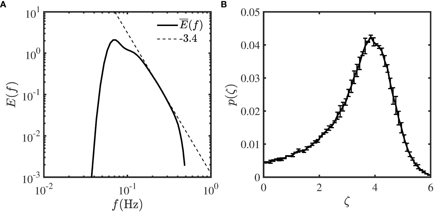
Figure 1 (A) Measured mean wave spectra collected by NDBC buoy 46086. (B) Measured PDF of scaling exponents in the wave spectra. The statistical difference between two subsets with equal sample size is indicated by error bar.

In such cases, the quadratic relation may not be valid (Resio et al., 1999). Indeed, if the f⁻⁵ spectrum in the PM64 theory is replaced by f^−ζ , where the exponent ζ can take different values, one obtains,

$\begin{array}{ll}E\left(f\right)=C_0{g}^2{\left(2\pi \right)}^{-4}{f}^{-\zeta }{e}^{-\frac{5}{4}{(\frac{f_m}{f})}^4}& (4)\end{array}$

According to the spectrum-based definition of Hs, Hs can be derived as,

$\begin{array}{ll}Hs=4\sqrt{\underset{\infty }{\overset{0}{\int }}E\left(f\right)df}& (5)\end{array}$

Note that f_m is also a cutoff frequency, e.g., E(f) is vanishing small for f≤f_m , thus,

$\begin{array}{ll}Hs\simeq 4\sqrt{\underset{\mathrm{fm}}{\overset{\infty }{\int }}E\left(f\right)df}=\sqrt{\frac{C_0}{\zeta -1}}\frac{g}{{\pi }^2}{f}_m^{-\frac{\zeta -1}{2}}& (6)\end{array}$

Finally, considering the relation between f_m and U₁₀, one obtains the wind wave relation as follows,

$\begin{array}{ll}Hs\left(U_{10}\right)\simeq \sqrt{\frac{C_0}{\zeta -1}}\frac{g}{{\pi }^2}{\left(\frac{0.855g}{2\pi }\right)}^{-\frac{\zeta -1}{2}}{U}_{10}^{\frac{\zeta -1}{2}}& (7)\end{array}$

Consequently, the scaling exponent β in the PM64-based wind-wave relation e.g.,

$\begin{array}{ll}Hs\left(U_{10}\right)=\alpha U_{10}^{\beta }& (8)\end{array}$

can be related to ζ as β=(ζ−1)/2. Using the observed range 3≤ζ≤6, one obtains β values in the range 1≤β≤2.5, which corresponds to a generalization of the quadratic law.

The ocean surface gravity waves are mixed products of swell and wind waves. For a better understanding of the relation between wind and waves, a separation of the swell and wind-wave should be considered. There are few choices to make this identification, when additional information is available. For example, the swell can be distinguished by an observer’s visual subjective criteria (Gulev et al., 1998; Gulev and Grigorieva, 2006), but the consistency and accuracy of such visual judgment results highly depend on the experience of the observer. Two objective approaches are also briefly discussed here. The first one is proposed in the framework of the wind-wave relation from the WAM model: Chen et al. (2002) defined the sea state of swell as the situations where the measured Hs is larger than the value predicted by this relation, while the wind waves correspond to the cases where the local measured Hs is smaller than the predicted value. However, as argued by Zheng et al. (2016), the “swell” defined by Chen et al. (2002) is still a sea state of mixed seas, thus the defined “swell” may be overestimated.

Another method which is supposed to be the best way to isolate swell from the wind-wave is the spectral partitioning (or Spectra Energy Partition, SEP) (Gerling, 1992; Hanson and Phillips, 2001; Wang and Hwang, 2001; Hanson and Jensen, 2004; Portilla et al., 2009; Hwang et al., 2012). As aforementioned, swell waves are conventionally thought as “old wind waves”, while the properties of swell waves depend strongly on their propagation history, and a continuous evolution can be detected associated with the distance travelled, life stages such as young, mature, old, etc. Consequently, a progressively clearer frequency could be detected in the wave spectrum to separate wind waves and swell waves. The SEP analysis has strict requirements for the data observations to generate the high frequency directional wave energy spectrum E(f,θ), which is used to describe the distribution of sea surface elevation variance as a function of wave frequency and wave propagation direction (θ). Besides, the wind direction (φ) and the wave phase speed c_p are also needed for the decomposition process. Based on the fact that the wave ages for wind wave and swell are different, the two different wave components can be distinguished in the wave energy spectrum by identifying a separation frequency f_s. For the WAM model, this critical frequency is defined as the frequency corresponding to the wave phase speed c=1.2×28×u_* cos (θ−φ), where the constant 1.2 is an empirical tuning parameter, 28 corresponds to the peak phase speed c_p=28u_*, and u_* is the friction velocity. Finally, the wind wave and swell parts can be estimated by integrating over the high and low frequency parts of the spectrum, respectively. The 2D wave spectrum is not easily obtained; for instance it can be estimated using a High Frequency radar and a buoy equipped with a digital directional wave module. Thus, it is difficult to apply the SEP algorithm to large-scale field observations, due to the lack of wave spectrum information. Nevertheless, SEP is popularly used in wave model data analysis. For the sake of its simplicity, a 1D frequency wave spectrum was developed and can also be used to do the swell identification. There are different ways to define the separation frequency in a 1D wave spectrum (Portilla et al., 2009). For example, f_s can be derived from the peak frequency f_m of the PM64 spectrum as, f_s=0.8f_m (Earle, 1984 Quentin, 2002). Additionally, Wang and Gilhousen (1998) proposed the wave steepness algorithm to extract f_s with a 1D wave spectrum-based wave steepness function. It was further developed by Gilhousen and Hervey (2002) with the consideration of U₁₀. The SEP method has been used by many authors to study the regional or global view of swell and wind wave features (Semedo et al., 2015; Zheng et al., 2016; Portilla-Yandun, 2018). Portilla et al. (2009) compared the performances of various spectral partitioning techniques and methods on the identification of wind waves and swells: significant differences have been found using different partitioning methods, and it was found that the existing spectral partitioning methods may deliver inconsistent output for wave systems. Moreover, the typical number of detected partitions in a measured spectrum is of the order of tens, and associating neighbor wave components at different times becomes intricate. It is therefore difficult to determine a clear frequency to separate the families of wind wave and swell (Gerling, 1992; Portilla et al., 2009).

To take into account the swell wave and to relax the FDS assumption, we propose in the present work a generalized power-law relation between local wind and waves. In the following, we first present the data and methods. Long-term buoy collected wind and wave data are used to verify the new swell identification method, and the local wind wave relation. The method is then validated by the SEP analysis. Then, the global patterns of the swell wave and the wind-wave relations are reported by using a 17-year of JASON altimeter calibrated wind and wave data. Finally, discussions and conclusions are addressed in last two sections.

2 Data

The in situ U₁₀ and Hs data from the NDBC are of high quality and have been extensively used for studying the wind wave interactions, validating model results and calibrating satellite systems (Ebuchi et al., 2002; Evans et al., 2003; Andreas and Wang, 2007; Zieger et al., 2015). Note that, the Hs is not directly estimated by sensors on board the buoys. The buoy-equipped accelerometers or inclinometers measure the heave acceleration or the vertical displacement of the buoy hull during the wave acquisition time. Then a fast Fourier transform is applied to the data to transform the temporal information into the frequency domain. After that, Hs is derived according to Equation (5) typically over the range from 0.0325 to 0.485 Hz.

The hourly averaged wind speed, significant wave height data provided by the NDBC buoy 46086 (located at 32.5^∘N and 118^∘W, with the water depth of 1844 m) for nearly 18 years (i.e., from 6 November 2003 to 31 December 2021) are used to illustrate the new swell identification method. The typical measurement accuracy for the NDBC buoy are 0.55 m/s and 0.2 m respectively for wind speed and significant wave height (Evans et al., 2003). Due to technical reasons, some data are missing, and there are a total of 149,089 valid pairs of wave height and wind speed values. The wind speed is measured by an anemometer located at z=4.1 m above the sea surface, a conversion from U_4.1 to U₁₀ is required before further studying the relation between wind and waves. Assuming that the marine atmospheric boundary layer is in a neutral stability logarithmic state, the surface wind profile is,

$\begin{array}{ll}{U}_z=\frac{u_{*}}{\kappa }\ln \frac{z}{z_0}& (9)\end{array}$

where κ is the von Kármán constant and z₀ is the roughness length, which is usually set as 0.4 and 9.7 ×10⁻⁵ m, respectively; z is the height above the sea surface; u_* is the friction velocity which can be experimentally derived from U₁₀ and the drag coefficient C_d (always set as 1.2 ×10⁻³) as follows,

$\begin{array}{ll}{u}_{*}=\sqrt{C_d}{U}_{10}& (10)\end{array}$

Combining the above two equations, U_z for z>0 can be re-expressed introducing U₁₀. By considering the measured wind speed at a height z₁ we finally have (Ribal and Young, 2019),

$\begin{array}{ll}{U}_{10}=U_{z_1}\sqrt{\frac{{\kappa }^2}{C_d}}\frac{1}{\text{ln} (z_1/z_0)}& (11)\end{array}$

Note that, to keep the self-consistency of this work, the parameters C_d and z₀ are the same as those in the second dataset (Ribal and Young, 2019). Finally, applying z₁=4.1 m in the above equation, the converted wind speed at 10 m can be expressed in a simplified way as U₁₀=1.084U_4.1. A further test shows that a variation of the height, e.g., 3≲z₁≲5  m, will have less than 2% difference in the estimation of U₁₀. Figures 2A, B show the hourly U₁₀ and Hs data collected by the NDBC buoy 46086, where annual cycles for wind speed and wave height are visible. Moreover, the corresponding hourly wave spectra with frequency on the range 0.02≤f≤0.485 Hz are also used to perform the SEP algorithm to retrieve the swell wave and wind waves: see the example of five days wave spectra during 27-31 December 2021 in Figure 2C. Two regimes are distinguished, the one with high frequency (e.g., f≥0.15 Hz) corresponds to the wind waves, and another one with low frequency (e.g., f≤0.15 Hz) indicates the swell waves.

FIGURE 2

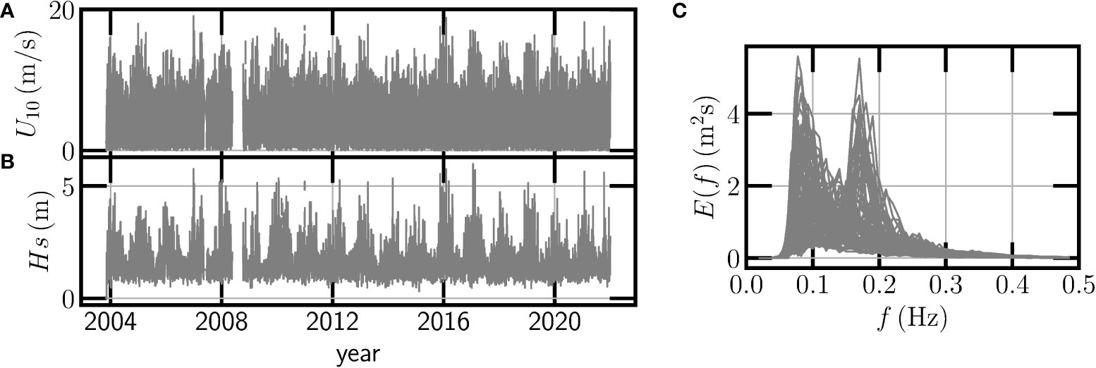
Figure 2 Illustration of the NDBC buoy 46086 collected hourly time series (A) U₁₀ and (B) Hs. (C) The collected wave spectra during 27-31 December 2021.

Another dataset is a 17-year (from 2002 to 2018) calibrated JASON altimeters observed global measurements of U₁₀ and Hs (Ribal and Young, 2019). Different pulses are received by the satellite altimeter, coming from reflections at the ocean’s surface. These different backscattered echos are classically treated using a model of the ocean’s rough surface (Brown, 1977), seen as the convolution of a point source, a flat sea surface, and an assumed probability density function of sea elevation. Based on the fitting of the Brown model echo to the recorded waveforms and the using of a maximum likelihood estimator, the Hs information could be retrieved. The U₁₀ is then estimated by a mathematical relationship with the backscatter coefficient and the Hs using the Gourrion algorithm (Gourrion et al., 2002) and Collard table (Collard, 2005). This dataset was carefully quality controlled and calibrated to ensure long-term stability and cross-mission consistency. The wind and wave data were archived in 1^∘×1^∘ bins in this dataset. It has been shown that this dataset agrees well with those provided by buoy and model reanalysis products (Young and Donelan, 2018; Takbash et al., 2019; Young and Ribal, 2019).

3 Method

3.1 Swell identification

As an example, here, we consider the empirical joint PDF p(U₁₀,Hs) for the wind and wave data collected by NDBC buoy 46086. The measured joint PDF is shown in Figure 3A, where 10 points are considered in each order of magnitude on a logarithmic scale. The conditional PDF of Hs for a given U₁₀ value possesses a well-defined maximum, which can be further confirmed by the individual normalized PDF curve for U₁₀≤4  m/s in Figure 3B, where the black solid curve is the average PDF. A well collapse of these PDFs is observed, indicating that in small wind conditions, the distribution of the measured Hs(U₁₀) are nearly independent of the local wind speed.

FIGURE 3

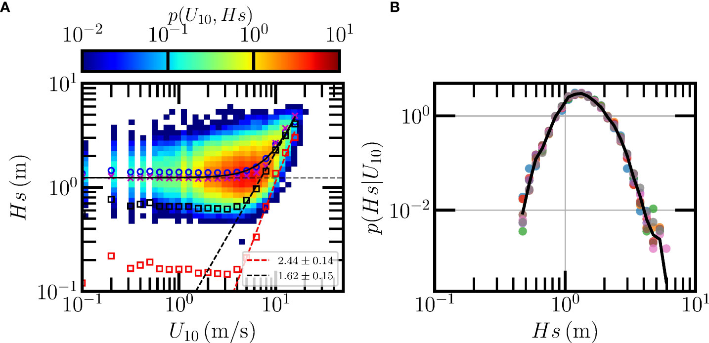
Figure 3 (A) Measured joint PDF of U₁₀ and Hs collected by NDBC buoy 46086, where the open circles (O) are the conditional mean $\overline{H}s\left(U_{10}\right)$; crosses (× ) are the skeleton Hs₀(U₁₀) of the joint PDF; the red squares and black squares are the local significant wave height $\overline{H}{s}_{Ll}\left(U_{10}\right)$ and $\overline{H}{s}_{Le}\left(U_{10}\right)$ derived via the linear decomposition and energy conservation approach, respectively. The dashed lines are the best fittings of the relation between $\overline{H}{s}_L\left(U_{10}\right)$ and U₁₀. The black solid curve is a reconstruction of the $\overline{H}s\left(U_{10}\right)$ based on Equation (16). (B) The conditional PDFs p(Hs|U₁₀) for Hs at small wind speeds, e.g., U₁₀≲4 m/s. The solid curve is the average PDF.

For a given U₁₀ value, we denote as Hs₀ the value of Hs corresponding to this maximum. This defines a new continuous curve, which is denoted as $\widehat{H}{s}_{sw}\left(U_{10}\right)$ with the following formulation,

$\begin{array}{ll}\widehat{H}{s}_{sw}\left(U_{10}\right)=H{s}_0;p\left(U_{10},H{s}_0\right)=\underset{Hs}{\max }\{p(Hs|U_{10})\}& (12)\end{array}$

This corresponds to a so-called skeleton of the joint PDF (Huang et al., 2008), illustrated as crosses in the figure. It is visible that $\widehat{H}{s}_{sw}\left(U_{10}\right)$ is nearly constant for light winds (e.g., U₁₀≲4 m/s), while increasing rapidly for strong winds (e.g., U₁₀≳4 m/s). Thus, it is reasonable to assume that in small wind conditions, the wave height is independent or weakly dependent on the local wind speed, and the local wave is surpassed by regular swell waves that have been generated from distant weather systems. Therefore, we propose here that Hs with maximum probability of Hs at small wind speeds, as the swell significant wave height. In the same figure, the conditional mean $\overline{H}s\left(U_{10}\right)={\int }^{}p\left(U_{10},hs\right)hsdhs$ is also represented and illustrated as circles (e.g.), in the figure. As aforementioned, the maximum probability of Hs(U₁₀) at a given small wind speed is either a constant or weakly dependent on the local wind, one thus can further determine the overall swell significant wave height $\overline{H}{s}_{sw}$ by averaging the almost constant values for low wind speeds,

$\begin{array}{ll}\overline{H}{s}_{sw}=⟨\widehat{H}{s}_{sw}\left(U_{10}\right){〉}_{U_{10}\le U_{cr}}& (13)\end{array}$

where 〈·〉 means average, U_cr is a critical wind speed (e.g., 4 m/s here), above which the local wind wave is then dominated. In this way, a constant swell value $\overline{H}{s}_{sw}$ is extracted from the data. For this case, $\overline{H}$s_sw is found to be 1.24 m.

3.2 Wind-wave identification

Ideally, the collected significant wave height Hs(U₁₀) at a certain local wind speed U₁₀ can be decomposed into two parts: i) the swell significant wave height Hs_sw that propagates from distant seas; ii) the local significant wave height Hs_L(U₁₀) generated by local winds. In the previous section, the average swell $\overline{H}{s}_{sw}$ is extracted by a probability-based approach, then two different wind-wave estimators are introduced here.

3.2.1 Linearly decomposed wind-wave

The first method to do the wind wave identification is based on the idea of linear decomposition. Let us assume that the collected waves are linearly composed by the swell and wind wave. Partially due to its simplicity, this assumption has been taken and used by many authors to construct the relation between wind and waves (Pandey et al., 1986; Chen et al., 2002; Andreas and Wang, 2007). In this way, the local significant wave height can be obtained by subtracting the swell value from the conditional mean as follows,

$\begin{array}{ll}\overline{H}{s}_{Ll}\left(U_{10}\right)=\overline{H}s\left(U_{10}\right)-\overline{H}{s}_{sw}& (14)\end{array}$

Here the subscript l is used to indicate the linearly decomposed local wind-wave. This quantity is represented in Figure 3A as red squares, where a power-law relation with the wind speed above U_cr is evident,

$\begin{array}{ll}\overline{H}{s}_{Ll}\left(U_{10}\right)={\alpha }_l{U}_{10}^{{\beta }_l};U_{10}>U_{cr}& (15)\end{array}$

where α_l=0.0044±0.0014 and β_l=2.44±0.14 are provided by the least square fit algorithm. Note that, as aforementioned, β_l can be different from the value of 2 for the FDS, see the red dashed line of the best fit curve in Figure 3A.

By doing so, that collected $\overline{H}s\left(U_{10}\right)$ can be decomposed into $\overline{H}{s}_{sw}$ and $\overline{H}{s}_{Ll}\left(U_{10}\right)$, the latter one can be related with U₁₀ using a power-law relation. Consequently, $\overline{H}s\left(U_{10}\right)$ is expressed as,

$\begin{array}{ll}\overline{H}s\left(U_{10}\right)=\overline{H}{s}_{sw}+{\alpha }_l{U}_{10}^{{\beta }_l}& (16)\end{array}$

The composite curve, i.e., $\overline{H}{s}_{sw}+{\alpha }_l{U}_{10}^{{\beta }_l}$ is shown as a black solid line in Figure 3A. Visually, this curve agrees well with the measured $\overline{H}s\left(U_{10}\right)$ when U₁₀≲20 m/s, with a relative error ⪅10% or a standard deviation ≃0.15 m. A more careful check shows an average relative error of 5% or a mean absolute error ≃0.1  m when 4≲U₁₀≲20 m/s. For U₁₀≲4 m/s, the reconstructed $\overline{H}s\left(U_{10}\right)$ is overlapped with $\overline{H}{s}_0\left(U_{10}\right)$. Moreover, it is interesting to see a sharp transition of the skeleton $\overline{H}{s}_0\left(U_{10}\right)$ roughly at U₁₀≃8 m/s, which confirms the above assumption that the swell wave dominates during the small winds.

3.2.2 Energy conserved wind-wave

As aforementioned, partially due to its simplicity, the measured significant wave height $\overline{H}s\left(U_{10}\right)$ is linearly associated with the swell $\overline{H}{s}_{sw}$ and the so-called local wind-wave $\overline{H}{s}_{Ll}\left(U_{10}\right)$, see Equation (14). According to ocean wave theory, in the meaning of the energy conservation, the total wave energy (i.e., $\overline{H}{s}^2\left(U_{10}\right)$) is equal to the sum of swell energy (i.e., $\overline{H}{s}_{sw}^2$) and local wind-wave energy (i.e., $\overline{H}{s}_L^2\left(U_{10}\right)$). This independence hypothesis might be violated by the above linear decomposition. To satisfy the energy conservation law, a strict analytical expression of the local significant wave height is written as,

$\begin{array}{ll}\overline{H}{s}_{Le}\left(U_{10}\right)=\sqrt{\overline{H}{s}^2\left(U_{10}\right)-\overline{H}{s}_{sw}^2}& (17)\end{array}$

where the subscript e is adopted here to indicate the wind waves that follow the energy conservation law. The experimental $\overline{H}{s}_{Le}\left(U_{10}\right)$ is shown as black squares in Figure 3A. A power-law behavior is observed in high winds as indicated by the black dashed line, which is expressed as,

$\begin{array}{ll}\overline{H}{s}_{Le}\left(U_{10}\right)={\alpha }_e{U}_{10}^{{\beta }_e};U_{10}>U_{cr}& (18)\end{array}$

For this case, the fitted value of β_e=1.62±0.15, is smaller than the previous one. The values of $\overline{H}{s}_{Le}$ are larger than the ones extracted by the linear decomposition method. The overall significant wave height $\overline{H}s\left(U_{10}\right)$ is then related with U₁₀ as,

$\begin{array}{ll}\overline{H}s\left(U_{10}\right)=\sqrt{\overline{H}{s}_{sw}^2+{\left({\alpha }_e{U}_{10}^{{\beta }_e}\right)}^2}& (19)\end{array}$

Furthermore, it is easy to obtain from Equations (16) and (19) the following relation,

$\begin{array}{ll}\overline{H}{s}_{Le}\left(U_{10}\right)\ge \overline{H}{s}_{Ll}\left(U_{10}\right)& (20)\end{array}$

Additionally for the high wind speed where the swell $\overline{H}{s}_{sw}$ can be ignored, the asymptotic behavior, i.e., $\overline{H}s\left(U_{10}\right)\simeq \overline{H}{s}_{Ll}\left(U_{10}\right)\simeq \overline{H}{s}_{Le}\left(U_{10}\right)$ can be safely applied, and one has

$\begin{array}{ll}{\beta }_l\ge {\beta }_e& (21)\end{array}$

This is partially due to the fact that for moderate wind speeds, the local wind wave $\overline{H}{s}_{Ll}\left(U_{10}\right)$ provided by the linear decomposition is smaller than $\overline{H}{s}_{Le}\left(U_{10}\right)$ provided by the energy conserved formula, see Equation (20). They should reach the same value of the significant wind wave height due to the asymptotic behavior. Therefore, the former one should grow faster than the latter one, indicated by the Equation (21), see an example in Figure 3.

3.3 Validation using the SEP algorithm

With the aforementioned probability analysis, a nominal swell $\overline{H}{s}_{sw}$ can be identified, thus the wind-wave $\overline{H}{s}_L\left(U_{10}\right)$. To verify the extracted swell and wind-wave, the SEP analysis is also performed for the wave partitioning of the data collected by the NDBC buoy 46086. The PM64-based algorithm (e.g., f_s=0.8f_m) is considered (Gilhousen and Hervey, 2002; Portilla et al., 2009). Note that when the wind speed is less than 2.1  m/s, the calculated f_s is then larger than 0.485  Hz. Therefore, in such cases no local wind-wave is extracted. The measured joint PDF of U₁₀ and Hs_sw(U₁₀) derived by the PM64-based SEP approach is shown in Figure 4A, in which the solid red curve is the conditional mean $\overline{H}{s}_{sw}\left(U_{10}\right)$, and the maximum statistical difference between two subsets with equal sample size is indicated by an error bar. It shows that there is roughly a constant value of $\overline{H}{s}_{sw}=1.24\pm 0.12$ m when U₁₀≲ 13 m/s, confirming the above assumption that in small wind conditions, the swell wave is independent or weakly dependent on the local wind speed. Note that the SEP-based $\overline{H}{s}_{sw}$ is coincidentally the same as the value of 1.24 m derived from the probability-based approach for the wind speed U₁₀≤4 m/s. A higher value $\overline{H}{s}_{sw}=1.35$ m is obtained when U₁₀≤5 m/s.

FIGURE 4

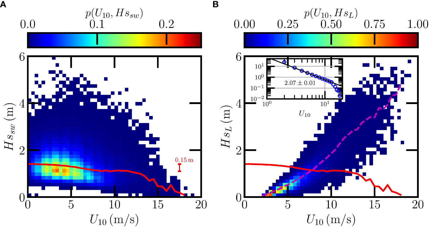
Figure 4 Measured joint PDFs of (A) U₁₀ and Hs_sw, and (B) U₁₀ and Hs_L extracted from the data provided by NDBC buoy 46086 with SEP analysis. The solid and dashed curves are the conditional average Hs_sw and Hs_L, respectively. The inset in (B) shows the ratio between $\overline{H}{s}_{sw}$ and $\overline{H}{s}_L$ at various wind speeds. The solid line indicates the best fit with the slope of −2.07. The maximum statistical difference between two subsets with equal sample size is indicated by an error bar in (A).

Figure 4B shows the joint PDF of U₁₀ and Hs_L, where the conditional mean wind wave $\overline{H}{s}_L\left(U_{10}\right)$ is illustrated by a dashed curve. To emphasize the assumption mentioned above that in small wind conditions the local wind wave is surpassed by the regular swell wave, the ratio between extracted swell wave $\overline{H}{s}_{sw}\left(U_{10}\right)$ and wind wave $\overline{H}{s}_L\left(U_{10}\right)$ is shown in the inset of Figure 4B in a log-log plot. It suggests that the swell wave dominates the collected significant wave height when U₁₀≪8 m/s. Moreover, a power-law decay for the ratio is found, in which an empirical exponent 2.07±0.01 is obtained. These results validate the assumption we made in the probability analysis, namely, that the measured Hs(U₁₀) is dominated by the swell wave for small wind conditions, and that the $\overline{H}{s}_{sw}\left(U_{10}\right)$ is nearly independent of the local wind, which is confirmed also by analyzing the data provided by other buoys (not shown here).

For comparison, the $\overline{H}{s}_{sw}\left(U_{10}\right)$ and $\overline{H}{s}_L\left(U_{10}\right)$ retrieved by our new probability-based methods and the SEP algorithm are reproduced in Figure 5. It shows that the measured $\overline{H}{s}_{sw}\left(U_{10}\right)$ (e.g., 1.35 m for U₁₀≤5 m) from the SEP is slightly larger than the one (e.g., 1.24 m) provided by the joint PDF in small winds. The above-mentioned two assumptions are well satisfied in small wind conditions. When U₁₀≥4 m/s, the SEP-based wind wave $\overline{H}{s}_L\left(U_{10}\right)$ are collapsing well with the $\overline{H}{s}_{Le}\left(U_{10}\right)$ provided by the energy-conserved decomposition. Power-law behavior is observed for the wind wave $\overline{H}{s}_L\left(U_{10}\right)$ provided by all three methods when U₁₀ exceeds 4 m/s with a scaling exponent β=1.69 for the SEP, a value β_l=2.44 is found for the linear decomposition approach, and β_e=1.62 for energy-conserved one.

FIGURE 5

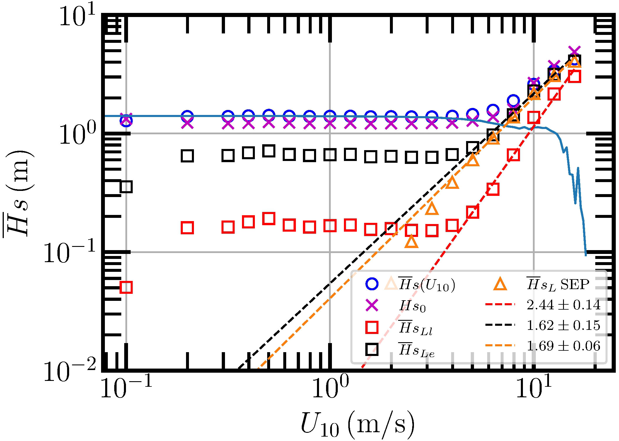
Figure 5 Comparison of the measured skeleton $\overline{H}{s}_0\left(U_{10}\right)$ (× ) for the joint PDF of U₁₀ and Hs provided by the NDBC buoy 46086. The extracted local significant wave heights $\overline{H}{s}_{Ll}\left(U_{10}\right)$ and $\overline{H}{s}_{Le}\left(U_{10}\right)$ by the probability-based approach is illustrated as □ . For comparison, the swell significant wave height $\overline{H}{s}_{sw}\left(U_{10}\right)$ (horizontal solid line) and local significant wave height $\overline{H}{s}_L\left(U_{10}\right)$ (△) extracted by the SEP approach are also shown. The dashed lines are the best fittings for the local significant wave height analysis.

With the proposed probability-based approach, the swell waves can be identified from the observed Hs(U₁₀) without the wave spectrum information. Consequently, the local wind-wave is defined by a linear decomposition or an energy conserved decomposition. After that, a power-law relation between the wind speed and the local wave is visible. One possible disadvantage of the probability-based method is that it requires a large number of data samples to construct the joint PDF p(U₁₀,Hs). The corresponding swell wave $\overline{H}{s}_{sw}$ is valid in an average sense. The main advantages of the current method are summarized as follows: i) only the overall significant wave height is needed when estimating the swell without knowing the wave spectrum a priori; ii) the influence of the anomalous values will be automatically excluded since they are in the tail of the PDFs; iii) the power-law relation between the local wind and waves is recovered for the high wind speeds for which the influence of the swell is nearly excluded.

4 Results

The buoy observations are often close to the coastal area, with few locations sampled over the global ocean, thus are spatially limited. To access global views of the swell and local wind-wave relation, satellite data are also used in this study. Here we combine the data collected by JASON-1 (from January 2002 to June 2013), JASON-2 (from July 2008 to July 2018), and JASON-3 (from February 2016 to July 2018) together (hereinafter referred to as JASON) to study the global distribution and seasonal variation of $\overline{H}{s}_{sw}$, and the relation between U₁₀ and $\overline{H}{s}_L\left(U_{10}\right)$. The calibrated data provided by Ribal and Young (2019) were archived in 1^∘×1^∘ bins. For enhancing the accuracy of the swell wave and local wave decomposition, the data are reassigned in 2^∘×2^∘ boxes. The data in the latitude coverage from 60^∘S to 60^∘N are considered for further analysis in this work.

4.1 Validation of JASON observations

Before processing the JASON data, the wind and wave data recorded by offshore NDBC buoys 41049 (located at 27.49^∘N, 62.94^∘W, with the water depth of 5,459 m) and 46006 (located at 40.77^∘N, 137.38^∘W, with the water depth of 4,323 m) are selected to perform comparisons with JASON observations, in order to examine the data quality. The joint PDFs for U₁₀ and Hs data observed by JASON in the area close to the buoys are estimated, then the skeleton of the joint PDF for the data provided by buoy and JASON are extracted, see Figure 6. The skeleton is overlapped under U₁₀≲ 6 m/s for both cases, except for a deviation found at U₁₀≃ 0.75 m/s for the second case: it might be induced by the uncertainty of satellite observations in extreme low wind conditions. According to the joint PDF, the $\overline{H}{s}_{sw}$ for NDBC buoy 41049, 46006 both equal to 1.25 m. The $\overline{H}{s}_{sw}$ extracted from JASON data which is close to the buoy 41049 is also 1.25 m, and the one corresponding to buoy 46006 is equal to 1.18 m.

FIGURE 6

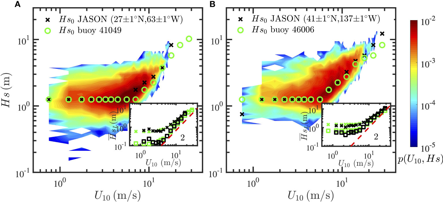
Figure 6 Measured joint PDFs of U₁₀ and Hs recorded by JASON in the areas close to NDBC buoys (A) 41049 and (B) 46006. The black crosses and green circles are the skeletons of the joint PDFs for JASON and buoy data. The insets show the measured $\overline{H}{s}_L$, in which the squares and crosses indicate the $\overline{H}{s}_{Ll}$ from linear decomposition and the $\overline{H}{s}_{Le}$ from energy conserved decomposition, respectively. The colors green and black are used to indicate the results from buoy and satellite data. The dashed line is given as a reference with the slope of 2.

The identified wind-wave is used to estimate the scaling exponents β for the local wind wave relation. Two decomposition methods are both used here, the results are illustrated in the insets in Figure 6, in which the squares and crosses are the wind-wave derived from the linear decomposition method and the energy conservation based approach, respectively. The colors green and black are used to indicate the results from buoy and satellite data. Visually, the derived wind waves are in a good agreement between the buoy and satellite observed data, where a similar scaling feature is obtained. More precisely, for the linear decomposition, the measured β_l for the data recorded by the buoy 41049 and nearby JASON data are 2.03 and 2.11; the results for the buoy 46006 and JASON data are 1.71 and 1.53. On the other hand, for the energy conservation approach β_e for the buoy 41049 and JASON data are 1.37 and 1.49; β_e for the buoy 46006 and JASON data are 1.25 and 1.22. These results show that the JASON data have remarkable performances in the swell identification and the construction of a local wind-wave relation.

4.2 Identified swell wave

The probability-based wave decomposition procedure is performed at each geographic grid to derive $\overline{H}{s}_{sw}$ and $\overline{H}{s}_L\left(U_{10}\right)$. To have a reasonable sampling size for each wind bin, we group the data into the four boreal seasons: Winter (DJF), Spring (MAM), Summer (JJA) and Autumn (SON). The derived swell is found on the range $0.5\le \overline{H}{s}_{sw}\le 4$ m, with a mean value around 1.8  m and a strong seasonal variation, see Figure 7. More precisely, the retrieved swell is stronger in the boreal Winter than in Summer in the Northern Hemisphere. For instance, the average $\overline{H}{s}_{sw}$ around 50^∘N are equal to 2.3 m and 1.2 m in DJF and JJA, respectively. This is partially due to the fact that the swell is highly positively correlated with the wind speed at high latitudes, see Figure 8, in which the black and red curves are the longitudinal averaged $\overline{H}{s}_{sw}$ and U₁₀, respectively. Similar meridional variation trends of $\overline{H}{s}_{sw}$ and U₁₀ are found, especially in high latitudes.

FIGURE 7

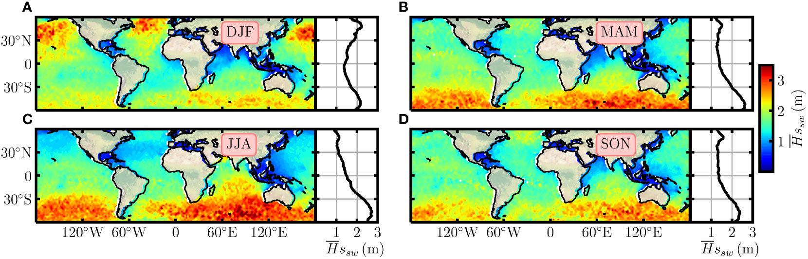
Figure 7 The global distributions of seasonal averaged $\overline{H}{s}_{sw}$ in (A) DJF, (B) MAM, (C) JJA, and (D) SON. The meridional variations are shown in the right panels.

FIGURE 8

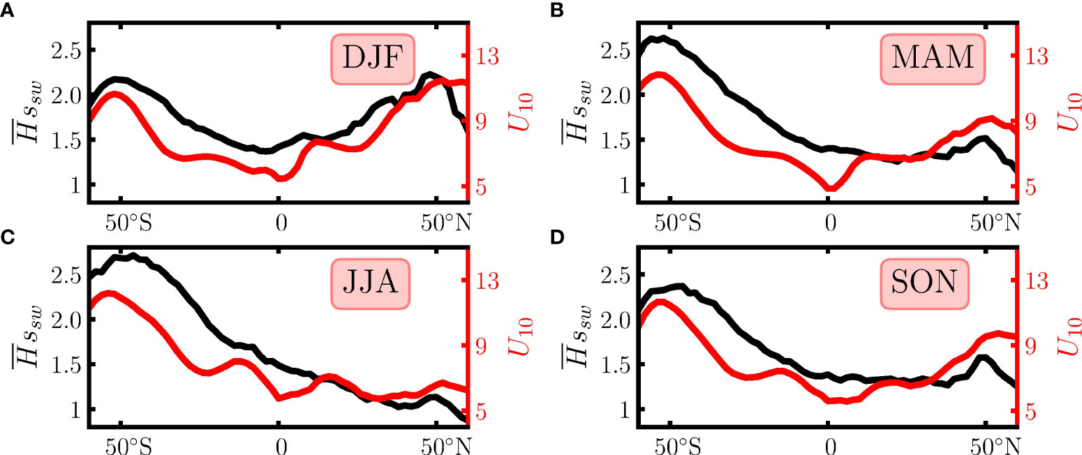
Figure 8 Meridional variations of $\overline{H}{s}_{sw}$ (black curve) and U₁₀ (red curve) in (A) DJF, (B) MAM, (C) JJA, and (D) SON.

The spatial patterns illustrated in Figure 7 agree well with the ones reported by Semedo et al. (2011). For example, in DJF, large swells are seen in the extratropical areas of the Northern Hemisphere, small ones are found in several regions, e.g., the Gulf of Mexico, Indian monsoon area, South China Sea, north and east coast of Australia, to list a few. Additionally, the longitudinal averaged curve shows a nearly symmetric shape, see Figure 7A. In the Southern Hemisphere, high values are mainly found in the Antarctic Circumpolar Current (ACC) region, i.e., roughly from 48^∘S to 58^∘S, where there is almost no influence of the continents. In JJA, the swell is increasing from the north to the south, reaching its maximum value in the ACC region.

4.3 Local wind wave relation

The local wind wave relation is described by a power-law formula in this study, e.g., $\overline{H}{s}_L\left(U_{10}\right)=\alpha U_{10}^{\beta }$, while different definitions of $\overline{H}{s}_L\left(U_{10}\right)$ correspond to distinct power-law features. In this section, the linear decomposition (i.e., Equation (14)) and energy conserved decomposition (i.e., Equation (17)) are both used to generate $\overline{H}{s}_L\left(U_{10}\right)$ with JASON data. The prefactor α and the scaling exponent β in the power-law relation is then estimated by using an automatic search algorithm with a width of half order of the wind speed magnitude above 4 m/s. The choice of a half order is due to the limited range of wind speed values. The global distribution of measured α in DJF and JJA are shown in Figure 9, in which Figures 9A, B are the ones fitted with linearly decomposed $\overline{H}{s}_{Ll}$; Figures 9C, D are the results from the $\overline{H}{s}_{Le}\left(U_{10}\right)$ estimated with energy conserved approach. The fitting algorithm fails on some geolocations due to the fact that the wind speed range is too short. This is observed in the small wind regions around the equator. The values of α_l extracted from $\overline{H}{s}_{Ll}\left(U_{10}\right)$ are smaller than the ones derived from $\overline{H}{s}_{Le}\left(U_{10}\right)$, the differences are around one order. However, as visible in the figures, the spatial patterns for α estimated from two defined $\overline{H}{s}_L\left(U_{10}\right)$ are similar, with small values in the equator and large ones in mid-latitudes. Moreover, seasonal differences are observed, relatively large α are found in the boreal Winter for the Northern Hemisphere.

FIGURE 9

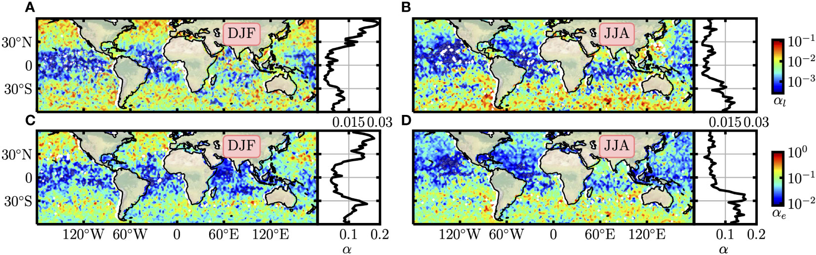
Figure 9 The global distributions of α_l measured with linearly decomposed $\overline{H}{s}_{Ll}$ in (A) DJF and (B) JJA. (C, D) are the α_e derived from the $\overline{H}{s}_{Le}$ decomposed by energy conservation theory. The meridional variations are shown in the right panels.

The corresponding measured β are shown in Figure 10. It is clear that the values of β_l derived from $\overline{H}{s}_{Ll}\left(U_{10}\right)$ (Figures 10A, B) are larger than the ones fitted with $\overline{H}{s}_{Le}\left(U_{10}\right)$ (Figures 10C, D), confirming the Equation (21). Linear decomposition based β_l are found close to the PM64 predicted value, e.g., 2 in the boreal winter for the Northern Hemisphere, where large winds are present. On the other hand, the values of β_e are close to 1.5 in DJF for the Northern Hemisphere. Moreover, seasonal variation and spatial differences for β are also found, large values of β are found mainly from 25^∘S to 25^∘N. The longitudinal averaged β is nearly symmetric in DJF, while is strongly asymmetric in JJA. Furthermore, opposite meridional variations for β are obtained as compared to the ones for α , large β values are found in low latitudes, corresponding to the areas with small winds.

FIGURE 10

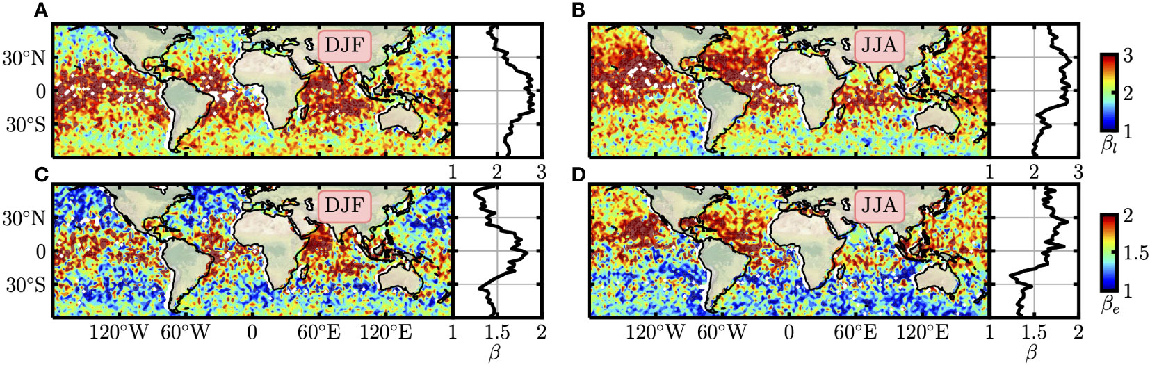
Figure 10 The global distributions of β_l measured with linearly decomposed $\overline{H}{s}_{Ll}$ in (A) DJF and (B) JJA. (C, D) are the β_e derived from the $\overline{H}{s}_{Le}$ decomposed by energy conserved approach. The meridional variations are shown in the right panels.

With the extracted swell $\overline{H}{s}_{sw}$, and α and β for the local wind wave, $\overline{H}{s}_L\left(U_{10}\right)$ can be predicted if the local wind U₁₀ is available. Here, the seasonal average U₁₀ is calculated for the JASON observation to predict $\overline{H}{s}_L$. The results in DJF and JJA are shown in Figure 11, in which Figures 11A, B are the ones derived with the power-law relations corresponding to the linear decomposed local wind waves, and Figures 11C, D are the ones estimated with the parameters from the energy conserved decomposition. The spatial and seasonal variation patterns are the same, with large $\overline{H}{s}_L$ occurring in mid-latitudes and in the boreal Winter for the Northern Hemisphere, except for the Somali coastal jet controlled region, where large $\overline{H}{s}_L$ are observed in JJA. The values of retrieved $\overline{H}{s}_{Ll}$ are smaller than $\overline{H}{s}_{Le}$. For instance, the measured $\overline{H}{s}_{Ll}$ in ACC are close to 1 m and 1.5 m in DJF and JJA, respectively. While the corresponding $\overline{H}{s}_{Le}$ in AAC are around 2.3 m and 3 m for the two seasons, respectively. Further comparison shows that the seasonal average $\overline{H}{s}_{Le}$ reproduced by the energy conservation-based theory are in good agreement with the ones reported by Semedo et al. (2011).

FIGURE 11

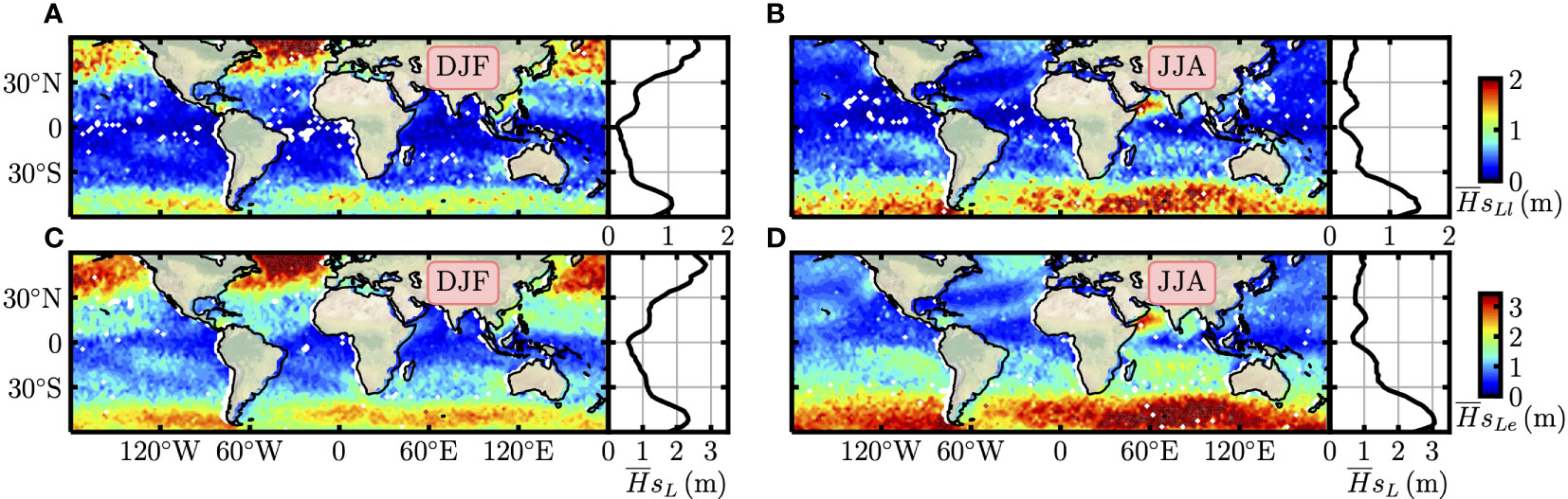
Figure 11 The global distributions $\overline{H}{s}_{Ll}$ predicted with the power-law models derived from linearly decomposed wind waves in (A) DJF and (B) JJA. (C, D) are the $\overline{H}{s}_{Le}$ estimated with the power-law models extracted from the wind waves decomposed by the energy conservation theory. The meridional variations are shown in the right panels. The model input U₁₀ is the seasonal averaged JASON wind.

4.4 Relation between α and β

The empirical PDFs of α and β are shown in Figure 12, in which Figures 12A, C are the PDFs for α_l and β_l , and Figures 12B, D are the ones for α_e and β_e , respectively. For the linear decomposed results, the most probable values (corresponding to the maximum of the PDFs) are α_l≃0.0065 and β_l≃2.11 . The latter one agrees well with the FDS’s prediction by Pierson and Moskowitz (1964), while the former value is found to be roughly one-fourth of their prediction. Globally, nearly one-third of the global ocean has values of β_l in the range of [1.8,2.2]. A longitudinal-averaged plot of the ratio for β_l values belonging to the range of [1.8,2.2] is shown in the inset of Figure 12C. Except for the boreal Summer, this ratio is nearly symmetric with large values in the high latitudes, and small values (e.g., less than 0.2 ) around the equator from 20^∘S to 20^∘N. A special case is observed for the Northern Hemisphere in JJA, for example, a mean value 0.18 is found from 20^∘N to 60^∘N, implying a strong influence of the monsoon. For the energy conserved decomposition, the most probable values for α_e and β_e are around 0.077 and 1.45, respectively, both significantly deviate from FDS’s prediction. The ratio of β_e in the range of [1.8,2.2] is also measured and shown in the inset in Figure 12D. The maxima of the ratio are found close to the equator, with the value of 0.2. Due to the effect of monsoon, the JJA case shows relatively large ratios in the Northern Hemisphere.

FIGURE 12

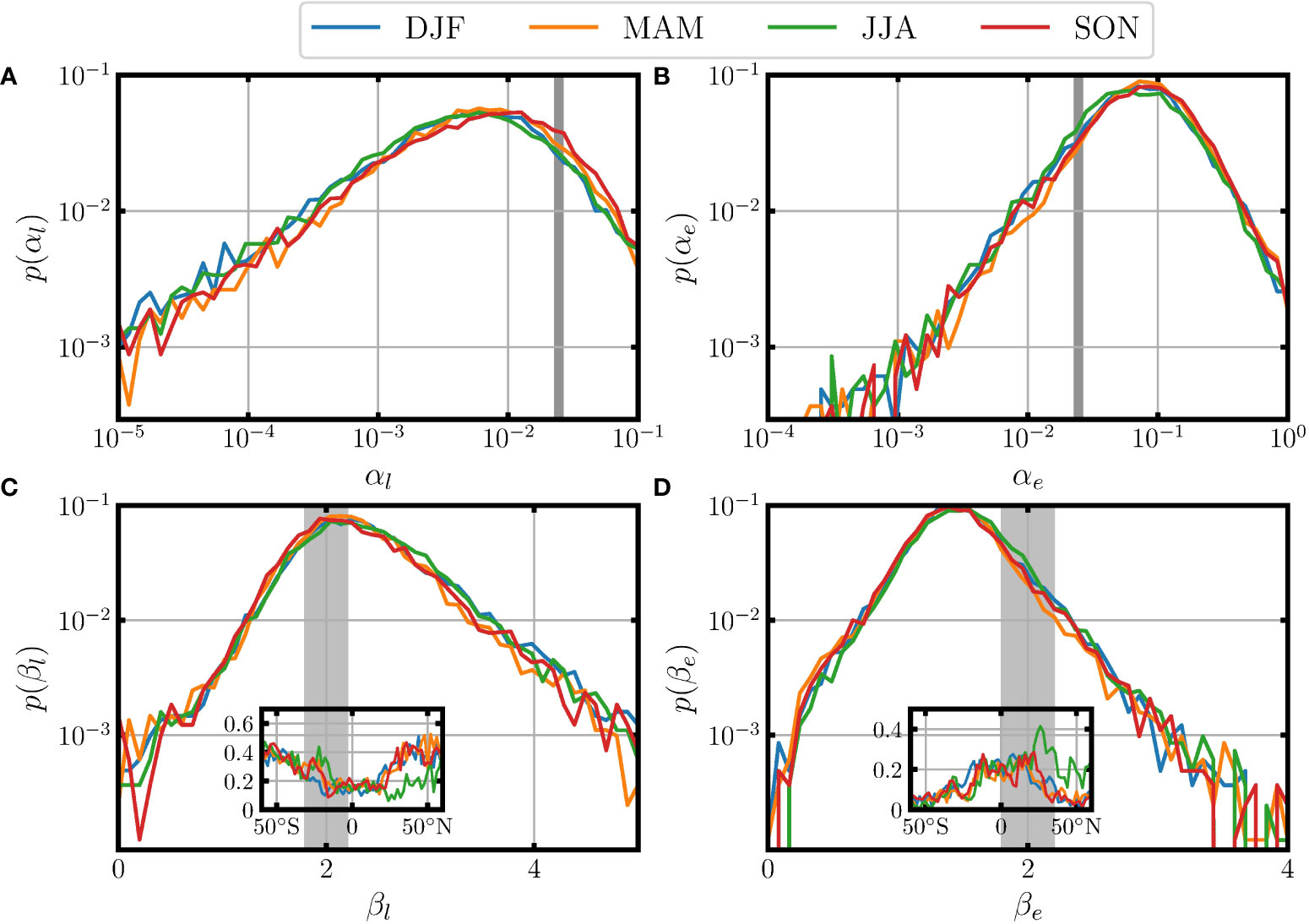
Figure 12 Measured PDFs for (A) α_l, (B) α_e, (C) β_l, and (D) β_e in four seasons. The insets in (C, D) are the ratios for β values in the range of [1.8,2.2] in various latitudes. The curves in different colors indicate different seasons.

To relate the derived α and β , phase diagrams α versus β are shown in Figures 13 in a semilog view, in which the PM64-based curve (see details in the discussion section) is also shown as a solid curve for comparison. It is interesting to see a nearly perfect exponential behavior, which is written as,

FIGURE 13

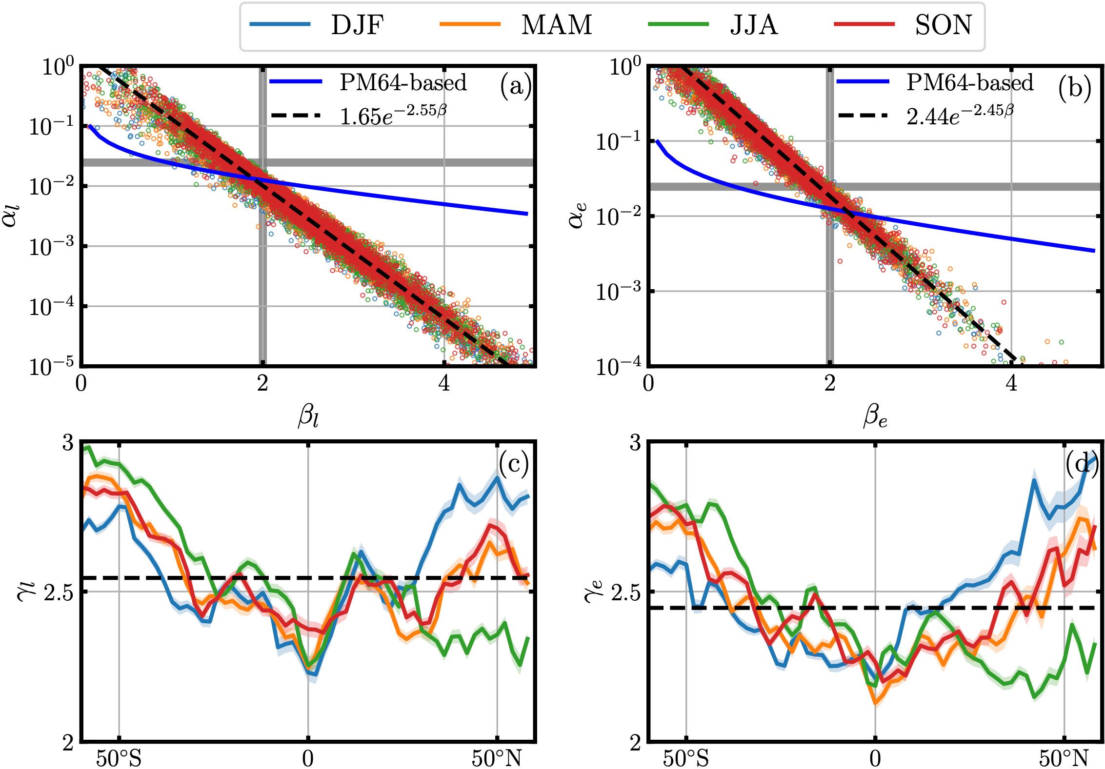
Figure 13 Relations between (A) α_l and β_l, (B) α_e and β_e. The dashed lines are the best fittings for the relation, the blue curve is the theoretical relation between α and β based on PM64 assumption. (C, D) are the meridional variations of the scaling exponents γ_l and γ_e, respectively, in which the dashed line is the average value.

$\begin{array}{ll}\alpha \left(\beta \right)=\omega e^{-\gamma \beta }& (22)\end{array}$

With the least square fitting algorithm, the exponential exponents are found to be ω_l=1.65 and γ_l=2.55. A further examination shows that the values of γ_l are latitude-dependent, e.g., a roughly linear decay is observed in the Southern Hemisphere from their maximum value of 3.0 to a minimum value of 2.25. It is then increasing linearly in the North Hemisphere. However, possibly due to the influence of the monsoon in the Northern Hemisphere, a strong seasonal variation is evident, e.g., a significant difference between the DJF and JJA cases is observed, a decreasing trend is found from 10^∘N to 60^∘N for measured γ_l in JJA. As for the energy conservation case, the fitted ω_e and γ_e are found with the values of 2.44 and 2.45, respectively. Hemispherical symmetric variations for γ_e are also found, with a linear decay from mid-latitudes to the equator, except for the one in the Northern Hemisphere in JJA.

5 Discussion

Without knowing the wave spectrum a priori, the proposed probability-based swell estimator relies on at least two closely related hypotheses: i) the observed significant wave height Hs(U₁₀) is dominated by the swell for the small wind condition and ii) the swell wave $\overline{H}{s}_{sw}\left(U_{10}\right)$ is either weakly dependent or independent of the local wind. These two hypotheses are confirmed by applying the SEP algorithm to the data, see Figure 4. The idea is tested and verified with buoy collected data, then extended to altimeter data. Note that the Hs measured from the buoy and altimeter are in two different ways, namely, buoy-derived and satellite-derived Hs possess conceptual differences. The altimeter data used in this study have been calibrated and validated against NDBC buoy data, the detailed processes can be found in Ribal and Young (2019). Though the concepts for Hs are different, the magnitudes are close to each other. Thus, the extension of the proposed method from buoy data to altimeter data is reasonable.

One advantage of the current proposal is that the influence of anomalous values will be automatically excluded since the skeleton of the joint PDFs is considered. However, to accurately estimate the skeleton (i.e., the nominal swell), a minimum sample size is required. One consequence is that the analysis is performed on a coarse time period, e.g., seasons in this study. Note that both the atmospheric and oceanic movements are driven either directly or indirectly by solar radiations. Therefore, daily and annual cycles due to earth rotation and revolution are expected. The former one is hard to be detected using the current satellite database since it requires a much larger dataset to capture the daily variation, while the latter one is confirmed by our results.

The swell $\overline{H}{s}_{sw}$ derived from the proposed probability-based method is validated against the SEP analysis, see the comparison between $\overline{H}{s}_0$ in small winds and $\overline{H}{s}_{sw}\left(U_{10}\right)$ extracted from SEP approach in Figure 5. Thus, the introduced new method can be used to distinguish the swell $\overline{H}{s}_{sw}$ from collected Hs(U₁₀) without knowing the wave spectra information a priori. The global view of $\overline{H}{s}_{sw}$ was then extracted for the 17-year JASON data. The extracted seasonal variations and spatial distribution pattern for $\overline{H}{s}_{sw}$ are the same as the ones extracted by the SEP analysis of reanalysis data (Semedo et al., 2011). For instance, large $\overline{H}{s}_{sw}$ are found in mid-latitudes during the boreal winter time, and the values of $\overline{H}{s}_{sw}$ in ACC are larger than 2 m.

The local wind-wave $\overline{H}{s}_L\left(U_{10}\right)$ are then identified by either the linear decomposition or energy conserved approach. The results show that the linearly decomposed $\overline{H}{s}_{Ll}\left(U_{10}\right)$ are smaller than the ones extracted based on energy conserved approach, see the Equation (20) and the experimental comparison in Figure 5. The latter one is overlapped with the extracted $\overline{H}{s}_L\left(U_{10}\right)$ from the SEP analysis in high winds since both of them are energy conserved. As illustrated by NDBC buoy data, the power-law relation of the local wind wave $\overline{H}{s}_L\left(U_{10}\right)$ against the local wind speed is recovered for the high values of the wind speed, e.g., U₁₀≥4 m/s, see Figure 3. To have the power-law behavior for at least half order range of wind speed, there should be enough data sample on the range 4≲U₁₀≲25  m/s. This condition might be not satisfied in small wind regions, e.g., the area around the equator, see Figures 9, 10. One possible solution is to fit the scaling exponent by using the fixed wind range, e.g., U₁₀≥4  m/s. Hopefully, with the accumulation of the observed products from the China France Oceanography SATellite (CFOSAT) data (Hauser et al., 2020), where the wind and waves are simultaneously collected, this difficulty will be overcome in the near future.

The fitted β_l for the linearly decomposed $\overline{H}{s}_{Ll}\left(U_{10}\right)$ are closer to the PM64 prediction. For instance, β_l values lie in the range of [1.8,2.2] over one-third of the global ocean. On the contrary, the β_e extracted with energy conservation based $\overline{H}{s}_{Le}\left(U_{10}\right)$ are relatively small, only a small portion have values close to 2. As for the prefactor α in the power-law relation, differences are also found between the two decomposed $\overline{H}{s}_L\left(U_{10}\right)$. The most probable value for α_l is found to be around 0.0065, and the one for α_e is to be around 0.077, one order of magnitude larger.

Moreover, an exponential relation is found between the prefactor α and the scaling exponent β in the proposed wind wave relation, see Figure 13. If one ignores the existence of the swell wave, the relation between α and β could be derived from PM64-like theory. Using β to substitute (ζ−1)/2 in the Equation (7), one obtains the following relation,

$\begin{array}{ll}\alpha \left(\beta \right)=\sqrt{\frac{C_0}{2\beta }}\frac{g}{{\pi }^2}{\left(\frac{0.855g}{2\pi }\right)}^{-\beta }& (23)\end{array}$

The corresponding PM64-based prediction of the relation between α and β is illustrated as solid curves in Figure 13, where an exponential behavior is found when β≳2. With the least square fit algorithm, the scaling exponent γ in the range 2≲β≲5 can be obtained with the value of 0.46, largely different from the measured ones. One possible reason is that the swell wave is excluded in this theoretical prediction. A more realistic model to take the swell into account is required in the future to explain this observed exponential relation.

With the above extracted wind wave power-law relation and the swell information, $\overline{H}s\left(U_{10}\right)$ can be predicted for a given U₁₀ via the synthesizing Equation (16) or (19). By considering its simplicity, the linear synthesizing Equation (16) is recommended to reconstruct $\overline{H}s$ here. For instance, using two years (from January 2020 to December 2021) annual average U₁₀ provided by CFOSAT (Figure 14A), the $\overline{H}s$ are calculated, see the global pattern of the model output in Figure 14C. The spatial pattern is very close to the CFOSAT observed one (Figure 14B): the differences between model output and observation are less than 0.3 m, see Figure 14D. More precisely, a relatively large discrepancy is found in mid-latitudes and a few nearshore regions around the equator. On the contrary, the differences are less than 0.3 m for most areas. More precisely, 88.1 % of the global oceans show differences within 0.25 m. Note that the accuracy for Hs measured by CFOSAT is 0.25-0.3 m or 5% of the mean value (Liu et al., 2020). Thus, the produced $\overline{H}s$ by the wind-wave model is in good agreement with satellite observation in an average sense.

FIGURE 14

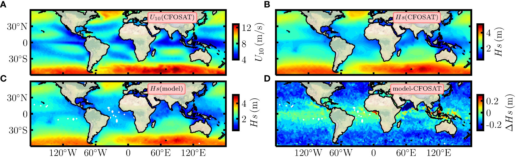
Figure 14 Annual average (A) U₁₀ and (B) Hs from CFOSAT observation. (C) Wind-wave power-law model generated Hs based on annual average U₁₀. (D) The differences between model results and observations.

For other applications, such as marine shipping or offshore industries, the real-time wave information is a key parameter with strong potential implications. In such a framework, the proposed wind wave relation model in this work could be used to predict the instantaneous wave height with the knowledge of the wind field. Here we show an example of using CFOSAT observed wind field on January 16, 2022 with a spatial resolution of 12.5 km to estimate the corresponding Hs, see Figure 15, where Figure 15A is the wind scatterometer observed U₁₀ (12.5 km spatial resolution, with the swath of 1000 km), Figure 15B the along-track Hs provided by the wave scatterometer with a spatial resolution of 1.5 km (Hauser et al., 2020) The model output significant wave height Hs is shown in Figure 15C. The spatial pattern for wave height is close to the one for wind speed. A comparison is made between CFOSAT observed along-track Hs (black dots) and the ones for model produced Hs (red dots) in Figure 15D. Similar meridional variations are found, the model results are close to the real observed ones for most latitudes, except for a small portion in low latitudes with a discrepancy around 0.5 m. The differences are acceptable for most regions when U₁₀≤12 m/s. Therefore, the model is suitable for moderate wind speeds to predict the instantaneous wave field. While the marine environment is complex, retrieved instantaneous wave height with the wind wave relation model may deviate systematically from the observations for the high-intensity wind speeds (figure not shown here). This systematical discrepancy is partially due to the underestimation of the high wind speed (Hauser et al., 2020). It might be corrected by either systematically checking the U₁₀ dependent bias or using a machine learning based model when the accumulation of the CFOSAT data is enough in the future.

FIGURE 15

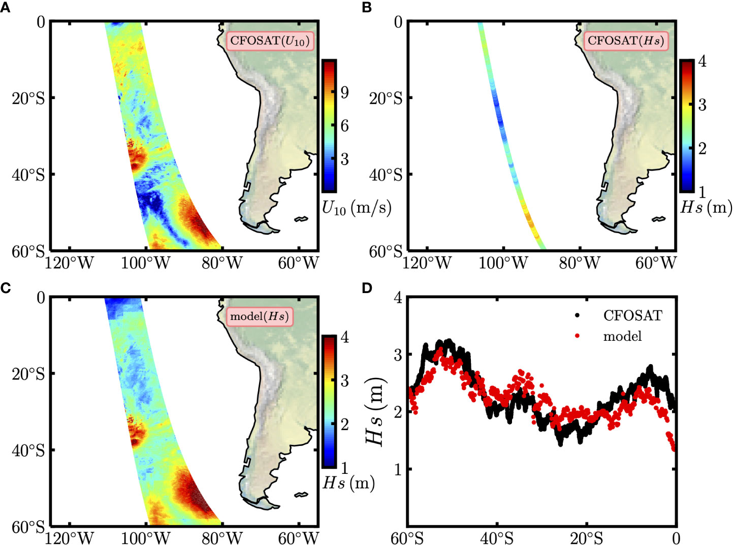
Figure 15 Simultaneously observed (A) U₁₀ and (B) Hs by the CFOSAT on January 16, 2022. (C) Wind-wave power-law model predicted Hs. (D) The meridional variations for CFOSAT along-track Hs (black dots) and the corresponding model predicted Hs (red dots).

6 Conclusions

In summary, a probability-based swell and local wind-wave decomposition is proposed in this work, which does not require the knowledge of the wave spectrum information a priori. Its methodology is first illustrated by the joint probability analysis of a buoy collected wind and wave data, then validated by a comparison with the classical SEP analysis using wave spectra data. The new method is then applied to the 17-year JASON data to retrieve the spatial and seasonal patterns of the swell. Both spatial and temporal patterns agree well with the previous study by Semedo et al. (2011). In this work, two different local wind-wave decomposition approaches are proposed. The first one is a linear decomposition, and the other one is based on an energy conservation hypothesis. Comparisons of the identified wind-wave by the two methods are made. It is shown that the $\overline{H}{s}_{Le}\left(U_{10}\right)$ extracted by the energy conservation based decomposition are close to the ones from SEP analysis, which can be explained by the fact that both are energy conserved approaches.

After the decomposition, a power-law formula of local significant wave height $\overline{H}{s}_L\left(U_{10}\right)$ against the local wind speed U₁₀ , e.g., $\overline{H}{s}_L\left(U_{10}\right)\propto U_{10}^{\beta }$, is advocated by relaxing the FDS hypothesis, where the scaling exponent β is treated as a free parameter. Global patterns of the derived β are presented for the first time. On average, the FDS hypothesis (with a scaling exponent equal to 2) might be satisfied in more than one-third of the oceans, according to the results derived by the linear decomposed $\overline{H}{s}_{Ll}\left(U_{10}\right)$: mainly in the ACC region, and in the high latitude of the Northern Hemisphere in the boreal winter time, where a strong wind is present. The exponent is largely deviating from the FDS’s prediction for the low latitude from 20^∘S to 20^∘N, where a weak wind is observed. On the contrary, the scaling exponents measured from the energy conserved approach $\overline{H}{s}_{Le}(U_{10}$ have relatively small values, with a most probable value of 1.45, which is not compatible with the FDS hypothesis.

Partially due to the influence of the monsoon and coverage of continents in the Northern Hemisphere, there is a strong seasonal variation for all parameters. For instance, in the Northern Hemisphere, the derived swell in JJA is much weaker than that in DJF (see Figure 7); the measured α in DJF is larger than the one in JJA (see Figure 9); the estimated β in JJA is larger than the one in DJF (see Figure 10). Furthermore, an exponential relation between the measured α and β is found, see Figure 13. A fine examination shows that the relation is latitudinal dependent, except for the boreal Summer case, and the exponent γ shows a linear decay from mid-latitudes to the equator, see Figure 13.

With the experimental wind wave relation in this work, a global view of $\overline{H}s$ can be obtained when only the wind speed is available. For example, with the annual average U₁₀, the corresponding global distribution of $\overline{H}s$ can be predicted, see Figure 14. The difference between the empirical model prediction and the so-called ground true value (e.g., the value provided by SWIM instrument of the CFOSAT satellite) is less than 0.3 m. Concerning instantaneous wave field prediction, the model output is quite accurate if the wind speed U₁₀ is correctly measured. Therefore, it can be hoped that, in the near future, with the accumulation of the simultaneous collected wind and wave information by the CFOSAT project, wind and waves can be mutually corrected via a machine learning based approach.

This work provides an efficient approach to identify the swell and the local wind wave. With the accumulation of satellite data, the spatial and temporal features of swell will be more precise and the wind-wave relation will be further improved in the future. We would like to provide a comment on the physical mechanism associated with the wind-wave relation. As aforementioned, the exact mechanism is still a mystery (Pizzo et al., 2021): for instance, there is still no theoretical interpretation of the empirical relation by considering first-principles and the effect of swell. A fully convincing theoretical consideration of the swell and local wave is still to be found, and empirical results such as obtained here could be useful in a such framework.

Data availability statement

Publicly available datasets were analyzed in this study. This data can be found here: www.ndbc.noaa.gov, https://portal.aodn.org.au/.

Author contributions

FS, JH, and YH conceived and designed the experiments. YG and YH performed the experiments and data analysis. YG and YH drafted the original manuscript, and FS and YH revised and edited the manuscript. All authors contributed to the article and approved the submitted version.

Funding

This work was supported by the National Natural Science Foundation of China (91958203, U22A20579 and 11732010). This research has been performed in the frame of the MultiW2 project, funded by the CNES/TOSCA program. Funding of YG’s Cotutella doctoral research project by Région Hauts-de-France and Xiamen University is acknowledged. YH is partially supported by State Key Laboratory of Ocean Engineering (Shanghai Jiao Tong University) (Grant No. 1910). A copy of Python codes to perform the analyses presented in this work can be found at https://github.com/lanlankai.

Conflict of interest

The authors declare that the research was conducted in the absence of any commercial or financial relationships that could be construed as a potential conflict of interest.

Publisher’s note

All claims expressed in this article are solely those of the authors and do not necessarily represent those of their affiliated organizations, or those of the publisher, the editors and the reviewers. Any product that may be evaluated in this article, or claim that may be made by its manufacturer, is not guaranteed or endorsed by the publisher.

References

Andreas E. L., Wang S. (2007). Predicting significant wave height off the northeast coast of the United States. Ocean Eng. 34, 1328–1335. doi: 10.1016/j.oceaneng.2006.08.004

CrossRef Full Text | Google Scholar

Babanin A. (2011). Breaking and dissipation of ocean surface waves (Cambridge, UK: Cambridge University Press).

Google Scholar

Bretschneider C. L. (1952). The generation and decay of wind waves in deep water. EOS Trans. Am. Geophys. Union 33, 381–389. doi: 10.1029/TR033i003p00381

CrossRef Full Text | Google Scholar

Brown G. (1977). The average impulse response of a rough surface and its applications. IEEE Trans. Antennas Propagation 25, 67–74. doi: 10.1109/TAP.1977.1141536

CrossRef Full Text | Google Scholar

Carter D. (1982). Prediction of wave height and period for a constant wind velocity using the JONSWAP results. Ocean Eng. 9, 17–33. doi: 10.1016/0029-8018(82)90042-7

CrossRef Full Text | Google Scholar

Cavaleri L., Abdalla S., Benetazzo A., Bertotti L., Bidlot J.-R., Breivik ø., et al. (2018). Wave modelling in coastal and inner seas. Prog. Oceanogr. 167, 164–233. doi: 10.1016/j.pocean.2018.03.010

CrossRef Full Text | Google Scholar

Chen G., Chapron B., Ezraty R., Vandemark D. (2002). A global view of swell and wind sea climate in the ocean by satellite altimeter and scatterometer. J. Atmos. Ocean. Technol. 19, 1849–1859. doi: 10.1175/1520-0426(2002)019<1849:AGVOSA>2.0.CO;2

CrossRef Full Text | Google Scholar

Collard F. (2005). Algorithmes de vent et période moyenne des vagues JASON à base de réseaux de neurons. Boost Technol.

Google Scholar

Csanady G. T. (2001). Air-sea interaction: laws and mechanisms (Cambridge, UK: Cambridge University Press).

Google Scholar

Donelan M. A., Hamilton J., Hui W. (1985). “Directional spectra of wind-generated ocean waves,” Philos. Trans. Roy. Soc. London 315, 509–562. doi: 10.1098/rsta.1985.0054

CrossRef Full Text | Google Scholar

Earle M. (1984). Development of algorithms for separation of sea and swell. (Hancock County: National Data Buoy Center Tech Rep MEC-87-1) 53, 1–53.

Google Scholar

Ebuchi N., Graber H. C., Caruso M. J. (2002). Evaluation of wind vectors observed by QuikSCAT/SeaWinds using ocean buoy data. J. Atmos. Ocean. Technol. 19, 2049–2062. doi: 10.1175/1520-0426(2002)019<2049:EOWVOB>2.0.CO;2

CrossRef Full Text | Google Scholar

Evans D., Conrad C., Paul F. (2003). Handbook of automated data quality control checks and procedures of the national data buoy center (Stennis Space Center, USA: NOAA National Data Buoy Center Tech. Document, 03–02).

Google Scholar

Faltinsen O. (1990). Wave loads on offshore structures. Annu. Rev. Fluid Mech. 22, 35–56. doi: 10.1146/annurev.fl.22.010190.000343

CrossRef Full Text | Google Scholar

Gao Y., Schmitt F. G., Hu J. Y., Huang Y. X. (2021). Scaling analysis of the China France oceanography satellite along-track wind and wave data. J. Geophys. Res. Oceans 126, e2020JC017119. doi: 10.1029/2020JC017119

CrossRef Full Text | Google Scholar

Gerling T. W. (1992). Partitioning sequences and arrays of directional ocean wave spectra into component wave systems. J. Atmos. Ocean. Technol. 9, 444–458. doi: 10.1175/1520-0426(1992)009<0444:PSAAOD>2.0.CO;2

CrossRef Full Text | Google Scholar

Gilhousen D. B., Hervey R. (2002). “Improved estimates of swell from moored buoys,” in Ocean wave measurement and analysis 2001 (Alexandria, VA, ASCE), 387–393.

Google Scholar

Goda Y. (1997). Directional wave spectrum and its engineering applications. Adv. Coast. Ocean Eng. 3, 67–102. doi: 10.1142/9789812797568_0003

CrossRef Full Text | Google Scholar

Gourrion J., Vandemark D., Bailey S., Chapron B., Gommenginger G., Challenor P., et al. (2002). A two-parameter wind speed algorithm for Ku-band altimeters. J. Atmos. Ocean. Technol. 19, 2030–2048. doi: 10.1175/1520-0426(2002)019<2030:ATPWSA>2.0.CO;2

CrossRef Full Text | Google Scholar

Gulev S. K., Cotton D., Sterl A. (1998). Intercomparison of the north Atlantic wave climatology from voluntary observing ships, satellite data and modelling. Phys. Chem. Earth 23, 587–592. doi: 10.1016/S0079-1946(98)00075-5

CrossRef Full Text | Google Scholar

Gulev S. K., Grigorieva V. (2006). Variability of the winter wind waves and swell in the north Atlantic and north Pacific as revealed by the voluntary observing ship data. J. Clim. 19, 5667–5685. doi: 10.1175/JCLI3936.1

CrossRef Full Text | Google Scholar

Hanson J. L., Jensen R. E. (2004). “Wave system diagnostics for numerical wave models,” in 8th international workshop on wave hindcasting and forecasting (Oahu, Hawaii: Citeseer), 231–238.

Google Scholar

Hanson J. L., Phillips O. M. (2001). Automated analysis of ocean surface directional wave spectra. J. Atmos. Ocean. Technol. 18, 277–293. doi: 10.1175/1520-0426(2001)018<0277:AAOOSD>2.0.CO;2

CrossRef Full Text | Google Scholar

Hasselmann K., Barnett T. P., Bouws E., Carlson H., Cartwright D. E., Enke K., et al. (1973). “Measurements of wind-wave growth and swell decay during the joint north Sea wave project (JONSWAP),” Dtsch. Hydrog. Z. Suppl. A 8.95 (Hamburg, Germany), pp. 8–12.

Google Scholar

Hauser D., Tourain C., Hermozo L., Alraddawi D., Aouf L., Chapron B., et al. (2020). “New observations from the SWIM radar on-board CFOSAT: Instrument validation and ocean wave measurement assessment,” IEEE Trans. Geosci. Remote Sens. 59, 5-26. doi: 10.1109/TGRS.2020.2994372

CrossRef Full Text | Google Scholar

Heimbach P., Hasselmann S., Hasselmann K. (1998). Statistical analysis and intercomparison of WAM model data with global ERS-1 SAR wave mode spectral retrievals over 3 years. J. Geophys. Res. Oceans 103, 7931–7977. doi: 10.1029/97JC03203

CrossRef Full Text | Google Scholar

Holthuijsen L. H. (2007). Waves in oceanic and coastal waters (Cambridge, UK: Cambridge University Press). doi: 10.1017/CBO9780511618536

CrossRef Full Text | Google Scholar

Huang Y., Schmitt F., Lu Z., Liu Y. (2008). An amplitude-frequency study of turbulent scaling intermittency using Hilbert spectral analysis. Europhys. Lett. 84, 40010. doi: 10.1209/0295-5075/84/40010

CrossRef Full Text | Google Scholar

Hwang P. A., Ocampo-Torres F. J., García-Nava H. (2012). Wind sea and swell separation of 1D wave spectrum by a spectrum integration method. J. Atmos. Ocean. Technol. 29, 116–128. doi: 10.1175/JTECH-D-11-00075.1

CrossRef Full Text | Google Scholar

Jones I. S., Toba Y. (2001). Wind stress over the ocean (Cambridge, UK: Cambridge University Press).

Google Scholar

Liu J., Lin W., Dong X., Lang S., Yun R., Zhu D., et al. (2020). First results from the rotating fan beam scatterometer onboard CFOSAT. IEEE Trans. Geosci. Remote Sens. 58, 8793–8806. doi: 10.1109/TGRS.2020.2990708

CrossRef Full Text | Google Scholar

Liu Y., Li S., Yi Q., Chen D. (2017). Wind profiles and wave spectra for potential wind farms in South China Sea. part II: Wave spectrum model. Energies 10, 127. doi: 10.3390/en10010127

CrossRef Full Text | Google Scholar

Pandey P., Gairola R., Gohil B. (1986). Wind-wave relationship from SeaSat radar altimeter data. Bound.-Layer Meteorol. 37, 263–269. doi: 10.1007/BF00122988

CrossRef Full Text | Google Scholar

Pierson J. W.J. (1991). Comment on “Effects of sea maturity on satellite altimeter measurements” by Roman e. glazman and Stuart h. pilorz. J. Geophys. Res. Oceans 96, 4973–4977. doi: 10.1029/90JC02532

CrossRef Full Text | Google Scholar

Pierson W. J., Marks W. (1952). The power spectrum analysis of ocean-wave records. EOS Trans. Am. Geophys. Union 33, 834–844. doi: 10.1029/TR033i006p00834

CrossRef Full Text | Google Scholar

Pierson J. W.J., Moskowitz L. (1964). A proposed spectral form for fully developed wind seas based on the similarity theory of S.A. kitaigorodskii. J. Geophys. Res. 69, 5181–5190. doi: 10.1029/JZ069i024p05181

CrossRef Full Text | Google Scholar

Pizzo N., Deike L., Ayet A. (2021). How does the wind generate waves? Phys. Today 74, 38–43. doi: 10.1063/PT.3.4880

CrossRef Full Text | Google Scholar

Portilla J., Ocampo-Torres F. J., Monbaliu J. (2009). Spectral partitioning and identification of wind sea and swell. J. Atmos. Ocean. Technol. 26, 107–122. doi: 10.1175/2008JTECHO609.1

CrossRef Full Text | Google Scholar

Portilla-Yandún J. (2018). The global signature of ocean wave spectra. Geophys. Res. Lett. 45, 267–276. doi: 10.1002/2017GL076431

CrossRef Full Text | Google Scholar

Quentin C. G. (2002). Study of the ocean surface, its radar signature and its interactions with turbulent momentum fluxes within the framework of the FETCH experiment. Ph.D. thesis, université Pierre and Marie curie-Paris VI.

Google Scholar

Resio D., Swail V. R., Jensen R. E., Cardone V. J. (1999). Wind speed scaling in fully developed seas. J. Phys. Oceanogr. 29, 1801–1811. doi: 10.1175/1520-0485(1999)029<1801:WSSIFD>2.0.CO;2

CrossRef Full Text | Google Scholar

Ribal A., Young I. R. (2019). 33 years of globally calibrated wave height and wind speed data based on altimeter observations. Sci. Data 6, 1–15. doi: 10.1038/s41597-019-0083-9

PubMed Abstract | CrossRef Full Text | Google Scholar

Romeiser R. (1993). Global validation of the wave model WAM over a one-year period using geosat wave height data. J. Geophys. Res. Oceans 98, 4713–4726. doi: 10.1029/92JC02258

CrossRef Full Text | Google Scholar

Rossby C.-G., Montgomery R. B. (1935). The layer of frictional influence in wind and ocean currents. Pap. Phys. Oceanogr. Meteor. 3, 1935-1904. doi: 10.1575/1912/1157

CrossRef Full Text | Google Scholar

Rusu L., Bernardino M., Guedes Soares C. (2014). Wind and wave modelling in the Black Sea. J. Oper. Oceanogr. 7, 5–20. doi: 10.1080/1755876X.2014.11020149

CrossRef Full Text | Google Scholar

Semedo A., Sušelj K., Rutgersson A., Sterl A. (2011). A global view on the wind sea and swell climate and variability from ERA-40. J. Clim. 24, 1461–1479. doi: 10.1175/2010JCLI3718.1

CrossRef Full Text | Google Scholar

Semedo A., Vettor R., Breivik Ø., Sterl A., Reistad M., Soares C. G., et al. (2015). The wind sea and swell waves climate in the Nordic Seas. Ocean Dyn. 65, 223–240. doi: 10.1007/s10236-014-0788-4semedo2015wind

CrossRef Full Text | Google Scholar

Sugianto D. N., Zainuri M., Darari A., Suripin S., Darsono S., Yuwono N. (2017). Wave height forecasting using measurement wind speed distribution equation in Java Sea, Indonesia. Int. J. Civ. Eng. Technol. Vol. 8, 604–619.

Google Scholar

Takbash A., Young I. R., Breivik Ø. (2019). Global wind speed and wave height extremes derived from long-duration satellite records. J. Clim. 32, 109–126. doi: 10.1175/JCLI-D-18-0520.1

CrossRef Full Text | Google Scholar

Toba Y. (1972). Local balance in the air-sea boundary processes. J. Oceanogr. 28, 109–120. doi: 10.1007/BF02109772

CrossRef Full Text | Google Scholar

Tucker M. J., Pitt E. G. (2001). Waves in ocean engineering Vol. 5 (Amsterdam: Elsevier).

Google Scholar

Villas Bôas A. B., Ardhuin F., Ayet A., Bourassa M. A., Brandt P., Chapron B., et al. (2019). Integrated observations of global surface winds, currents, and waves: Requirements and challenges for the next decade. Front. Mar. Sci. 6 425. doi: 10.3389/fmars.2019.00425

CrossRef Full Text | Google Scholar

WAMDI Group (1988). The WAM model–a third generation ocean wave prediction model. J. Phys. Oceanogr. 18, 1775–1810. doi: 10.1175/1520-0485(1988)018<1775:TWMTGO>2.0.CO;2

CrossRef Full Text | Google Scholar

Wang D., Gilhousen D. (1998). “Separation of seas and swells from NDBC buoy wave data,” in Fifth int. workshop on wave hindcasting and forecasting (Florida, FL, ASCE: Environment Canada Melbourne), 155–162.

Google Scholar

Wang D. W., Hwang P. A. (2001). An operational method for separating wind sea and swell from ocean wave spectra. J. Atmos. Ocean. Technol. 18, 2052–2062. doi: 10.1175/1520-0426(2001)018<2052:AOMFSW>2.0.CO;2

CrossRef Full Text | Google Scholar

Wen S. C. (1960). Generalized wind wave spectra and their applications. Scientia Sin. 9, 377–402. doi: 10.1360/ya1960-9-3-377wen1960generalized

CrossRef Full Text | Google Scholar

Wu J. (1968). Laboratory studies of wind–wave interactions. J. Fluid Mech. 34, 91–111. doi: 10.1017/S0022112068001783

CrossRef Full Text | Google Scholar

Young I. R. (1998). Observations of the spectra of hurricane generated waves. Ocean Eng. 25, 261–276. doi: 10.1016/S0029-8018(97)00011-5

CrossRef Full Text | Google Scholar

Young I. R., Donelan M. (2018). On the determination of global ocean wind and wave climate from satellite observations. Remote Sens. Environ. 215, 228–241. doi: 10.1016/j.rse.2018.06.006

CrossRef Full Text | Google Scholar

Young I. R., Ribal A. (2019). Multiplatform evaluation of global trends in wind speed and wave height. Science 364, 548–552. doi: 10.1126/science.aav9527

PubMed Abstract | CrossRef Full Text | Google Scholar

Young I. R., Verhagen L. (1996). The growth of fetch limited waves in water of finite depth. part 2. Spectral evolution. Coast. Eng. 29, 79–99. doi: 10.1016/S0378-3839(96)00007-5

CrossRef Full Text | Google Scholar

Zhang F. W., Drennan W. M., Haus B. K., Graber H. C. (2009). On wind-wave-current interactions during the shoaling waves experiment. J. Geophys. Res. Oceans, 114. doi: 10.1029/2008JC004998

CrossRef Full Text | Google Scholar

Zheng K., Sun J., Guan C., Shao W. (2016). Analysis of the global swell and wind sea energy distribution using WAVEWATCH III. Adv. Meteorol. 2016, 8419580. doi: 10.1155/2016/8419580

CrossRef Full Text | Google Scholar

Zieger S., Babanin A. V., Rogers W. E., Young I. R. (2015). Observation-based source terms in the third-generation wave model WAVEWATCH. Ocean Model. 96, 2–25. doi: 10.1016/j.ocemod.2015.07.014

CrossRef Full Text | Google Scholar