 Kangzhuang Liang
 Wei Li1,2,3*
 Guijun Han
 Xuan Wang
- 1Tianjin Key Laboratory for Oceanic Meteorology, Tianjin, China
- 2Tianjin Institute of Meteorological Science, Tianjin, China
- 3School of Marine Science and Technology, Tianjin University, Tianjin, China
The analytical four-dimensional ensemble variational (A-4DEnVar) data assimilation scheme inherits the advantages of the conventional four-dimensional variational (4D-Var) data assimilation scheme and removes the adjoint model. However, compatible operational improvements such as the reduction of the computational costs and the localization method should be considered when it is used in realistic systems. In this paper, the computational complexity of calculating the inverse of background error covariance (the B matrix) is decreased by a precondition transform method, i.e., introducing a new state variable whose product with the B matrix is the original state variable to be optimized in the cost function. Furthermore, an independent point (IP) scheme is combined to construct an implicit localization method and further decreases the computational cost. Based on the Princeton Ocean Model with the generalized coordinate system (POMgcs), the operational improved A-4DEnVar is applied to optimize the spatially varying bottom friction coefficients (BFCs) of the M2 constituent in the Bohai and Yellow seas. A twin experiment with idealized observations is designed to validate the effectiveness of the proposed method. In practical experiments, with no more than 10 IPs, the algorithm can assimilate observations from the National Astronomical Observatory (NAO) dataset and obtain a good simulation. The experimental performances increase with the increase of either the IPs or observations, which indicates the efficacy of the proposed algorithm.
1. Introduction
Modern numerical weather prediction (NWP) and/or ocean prediction suffer from the uncertainty of initial conditions and parameters in numerical models. Data assimilation methods are widely implemented to provide better initial fields and parameters by blending numerical models with information extracted from a variety of observations. The four-dimensional variational data assimilation method (4D-Var, Courtier and Talagrand, 1987; Talagrand and Courtier, 1987; Rabier et al., 2000; Stammer et al., 2002; Rawlins et al., 2007 and Wunsch and Heimbach, 2013) and ensemble Kalman filter (EnKF) are two major advanced data assimilation methods (Evensen, 1994; Evensen, 2004). They have been successfully applied in many operational centers, and both of them have great characteristics (Kalnay et al., 2007; Buehner et al., 2010a; Buehner et al., 2010b). As a non-sequential data assimilation method, 4D-Var can assimilate asynchronous observations so that the analysis results from 4D-Var are continuous in a long data assimilation window. Developed from the Kalman filter and extended Kalman filter, EnKF benefits from the estimation of a flow-dependent analysis error covariance. However, the two well-accepted powerful data assimilation schemes are also hampered by their deficiencies. On the one hand, a defection for 4D-Var is its high dependency on the adjoint model (of the forecast model) that usually costs a lot of human resources and is difficult to maintain or transplant to other systems. Furthermore, the lack of flow-dependent background error covariance (denoted as B) reduces the performance of 4D-Var. On the other hand, by considering observations sequentially, the EnKF can hardly assimilate all observations spread in a long data assimilation window simultaneously. The discontinuous analysis fields are not consistent with the natural facts.
A suite of cutting-edge hybrid data assimilation methods has been proposed to possess the advantages of 4D-Var and EnKF and avoid their disadvantages. En4DVar and 4DEnVar methods are both outstanding schemes of them (Goodliff et al., 2015; Lorenc et al., 2015; Liu and Xue, 2016). The En4DVar constructs the B matrix as a linear combination of a static part with a flow-dependent part estimated from ensemble members (Buehner, 2005). Since it retains the structure of 4D-Var, the adjoint model is also necessary for the En4DVar scheme. The 4DEnVar is devoted to not only introduce a flow-dependent B matrix into the form of 4D-Var but also remove the adjoint model. To this end, the 4DEnVar utilizes some ensemble perturbation evolutions to approximate the tangent linear model. Liu et al. (2008; 2009) and Liu and Xiao (2013) proposed the primary formulation of the 4DEnVar in which the analysis field is a linear combination of the ensemble mean with observation perturbations. Other studies like Tian et al. (2018) noticed the shortcomings of the 4DEnVar schemes that the ensemble members and thereby the values of the adjoint model are unchanged in iteration loops. To improve the performance, Tian et al. (2018) proposed a series of non-linear least squares En4DVar (NLSi-En4DVar) methods. Especially, the fifth variant (NLS5-En4DVar) is a so-called iterative improvement scheme. NLS5-En4DVar is composed of inner loops and outer loops in which the conventional 4DEnVar and update of ensemble members are implemented, respectively. A multigrid scheme is also developed in Zhang and Tian (2018). The ill-posedness of the inverse problem caused by the increase of the number of variables to be estimated or optimized should be eliminated by reducing the dimensions of variables or introducing useful regularizations. Nowadays, Tian and Zhang (2019a); Tian and Zhang (2019b) studied the generation of ensemble members and expanded the cost function with a regularization (Tian et al., 2020). The most significant superiority of the 4DEnVar schemes beyond others is that it inherits the performance of the conventional 4D-Var and avoids the usage of the adjoint model. As assumed explicitly or implicitly in the above studies, to estimate a reasonable adjoint model, the ensemble perturbations need to be as small as possible. Large perturbations are not compatible with the framework of the 4DEnVar schemes. However, in these above works, the ensemble covariance is set to be the same as the B matrix like EnKF does. To overcome this drawback, Liang et al. (2021) constructed the ensemble covariance by multiplying a small scaling factor (denoted as μ) to the B matrix. It is demonstrated that only if the scaling factor is less than 10-6 for the Lorenz-63 model, the value of the adjoint model and the gradients estimated by ensemble members would be close enough to the value obtained from the conventional 4D-Var. Otherwise, the assertion that 4DEnVar is equivalent to the conventional 4D-Var only holds for short data assimilation windows where the non-linearity is limited. Compared to other schemes, A-4DEnVar proposed by Liang et al. (2021) is a more rigorous framework. The superiority of the method has been proven not only in theory but also in ideal twin experiments, especially with long data assimilation windows.
Beyond these advantages, A-4DEnVar lacks of discussions in realistic models. In practice, the dimensions of the state variables in operational systems are often large. For ensemble-based methods, operational improvements and/or modifications are necessary to avoid the high computational cost of the inverse of the B matrix and restrain the spurious correlations caused by insufficient ensemble members. For the first issue, to remove the inverse of the B matrix, the usual process is introducing a new state variable, denoted as ω, for example, and preconditioning the cost function using the transformation (Oddo et al., 2016; Storto et al., 2018) or , where is the state variables or perturbations in the physical space. For the second issue, a straightforward way to eliminate the spurious correlations is to modify the background error covariance matrix through a localization operator or function. Some improvements and variants are also studied. Liu et al. (2009) proposed a reasonable localization approach through multiplying ensemble members by the first M empirical orthogonal functions (EOFs) of the Schur operator. Although the approach is well accepted in ensemble-based algorithms, the necessary computational cost increases because it increases the ensemble size by M times. Despite the above methods, some simple and convenient strategies are enlightening. One of these methods, the so-called independent point (IP) or feature point (FP) scheme, is proposed in the studies of Zhang and Lu (2008); Zhang and Lu (2010) and Zhang et al. (2011) and is used in Zhang and Wang (2014); Guo et al. (2017), and Qian et al. (2021) to optimize the open-boundary conditions of tidal currents and/or bottom friction coefficients (BFCs) of the tidal constituent. In this scheme, only the values of several selected nodes are optimized, and the value of other rest nodes is calculated by Cressman linear interpolation. As they demonstrated, both the dimension of the parameter space and the ill-posedness of inverse problems are reduced. Apparently, the IPs scheme is easy to implement, especially for the estimation of spatially or temporally distributed parameters. Pan et al. (2017) discussed the IP interpolation methods in detail. While the conventional adjoint method is implemented in the above studies, a natural question is how to integrate this convenient approach into A-4DEnVar and exploit its ability on some realistic operational systems.
We address the above questions in this paper. We not only constructed an operational improvement variant of A-4DEnVar with a precondition transformation but also combined it with the IP scheme and explored its potential for the BFC estimation problems. At the beginning of the paper, the preconditioning transformation is introduced to A-4DEnVar to avoid the inverse of the B matrix. The algorithm is decomposed as inner and outer loops to further improve its ease of implementation. Following the derivation and combining with the IP scheme, we estimate the spatially varying BFCs using the newly improved variant. The estimation is based on the external mode of the Princeton Ocean Model general coordinate system (POMgcs, Ezer and Mellor, 2004), which is, in fact, a two-dimensional shallow water equation. The effectiveness and good performance of A-4DEnVar are validated by a twin experiment with some known and randomly chosen BFCs. A practical experiment in which the sea-level evaluation observations are generated from the NAO (Matsumoto et al., 2000) tidal harmonic constant datasets (https://www.miz.nao.ac.jp/staffs/nao99/data/nao99Jb.tar.gz) is implemented to investigate the distribution of BFCs in the Bohai and Yellow seas.
The remainder of this paper is organized as follows. In section 2, the formulations and derivations of the operational improved variant algorithm are described in detail. Section 3 introduces the numerical model and datasets. The data assimilation experiment setups and their results are shown in section 4. The last section lists the discussions and conclusions of this study.
2. Methodology
2.1. Preconditioning of the cost function
For the conventional 4D-Var scheme, the cost function is defined as
where x0 and λ are the initial conditions and the parameters in dynamic models. xb and B are the background initial conditions and the corresponding background error covariance. Here, a priori or background parameter λb and error covariance C are also included for the combined estimation problem, but they are not always explicit in practice. The dynamic model evolving from t0 to ti is denoted as ℳi =. The observation operator at time step ti is ℋi . yi and Ri are the observations and their error covariances, respectively. Although the cost function mentioned above contains the estimation of the initial conditions and parameters simultaneously, it is convenient to reconstruct it to the estimation problems in which only initial condition or parameters are considered. However, to simplify the descriptions below, we consider Equation 1 directly and without any modifications for both initial condition estimation and parameter estimation problems.
The cost function in A-4DEnVar is similar with that in conventional 4D-Var except for the expression of independent variables that are composed of an approximation of the truth (denoted as and λ*) and their perturbations (denoted as and ) to better illustrate an iterative algorithm. That is
If there are no precondition processes, a straight way to obtain the minimum of the cost function is to calculate its gradient as done in the original A-4DEnVar. In the initial optimization problems, for the fixed , the gradient of the cost function with respect to perturbations are
Due to the large dimensions of the background error covariances, accurate calculations for the inverse matrix B-1 require a lot of computational resources. If the localizations are not considered, an elegant way is to estimate them with the covariances of several (often less than 100) ensemble members so that the inverse is, in fact, replaced with the pseudo-inverse matrix [see the appendix of Liang et al. (2021) for details)]. However, localizations play a significant role in the construction of the background error covariances and are often irreplaceable in operational systems to eliminate the long-distance pseudo-correlations. The elegant way would introduce some unexpected errors into gradient. Similar questions also exist in parameter estimations if the dimension of parameters is large. A convenient way is to remove the inverse matrix in Equations 2 and 3 through a precondition process as described below.
To avoid the calculation of the inverse of B, one often preconditions the independent variable using . The cost function is hence expressed as
In fact, the terms corresponding to the parameters are treated as constants in the initial condition estimation problem. The gradient of the cost function is
where Hi denotes the tangent linear model of the observation operator ℋi. It should be noted that the value of tangent linear model and, hence, the structure of cost function depends on , the prior approximation of the truth. Thus, to achieve the minimization of the cost function in Equation 1, should be updated iteratively.
Since is a small perturbation, the Taylor expansions of the dynamic model operators indicate that
or it can be further simplified as
in which is the tangent linear model of ℳi. Equation 7 provides an efficient way to estimate the tangent linear model. The processes are similar to what was mentioned in Liang et al. (2021). Once there are N sufficient samples of and , denoted as and respectively, the tangent linear model satisfies
The least squares estimation of the tangent linear model is
if the dimension of state variables is not large and is full rank. It is clear that for different (although the is different in this situation), Equations 8 and 9 are satisfied. Thus, the generation of ensemble does not influence the estimation of the tangent linear models and adjoint models. Otherwise,
where a pseudo-inverse of denoted as is adopted. In this situation, the estimations of tangent linear models are different with the difference of space generated by ensemble members. The widely used EOFs should be used to construct reasonable ensembles. However, due to the fact that the IP scheme is adopted in this paper, this situation is avoided actually. Substituting the into Equation 5 yields the estimation of the gradient
Equation 11 is the gradient of cost functions with respect to the precondition variables in the initial condition optimization problems. The construction details of are related to the generation of the ensemble members, which will be discussed in the next subsections.
For the parameter estimation, the processes and derivations are similar as what was derived in the initial condition estimation except for some details. Set parameters are composed of prior components and perturbation components. That is
and, again, assume that
The parameter perturbations have
where the tangent linear model is about the parameter variables λ*.
Let
be a matrix with N samples of as its columns and their corresponding state variable perturbations also be composed of a matrix named as . Then, the estimation of
Mi|λ* is
when the is full rank. Otherwise, the estimation is
where is the pseudo-inverse of .
The cost function for parameter estimation is expressed as
The gradient with respect to ω is
Again, the generation of ensemble members will be discussed in the next sections.
Since the gradients are obtained, combining with a suitable optimization method [e.g., the linear research gradient descent method, the Newton descent method, and the limited-memory quasi-Newton method (L-BFGS) method], the minimization of the cost function can be calculated.
2.2. Generation of the ensemble perturbations
In subsection 2.1, we presented the framework of A-4DEnVar with precondition variables. The remaining question is how to generate reasonable ensemble perturbations in practice. To ensure an accurate estimation of tangent linear models in Equations 10 and 16, the basic assumption is that the magnitudes of perturbations should be much smaller than that of independent variables. It must be mentioned that the errors generated by a probability density distribution with the covariance B (for initial estimation) or C. (for parameter estimation) are usually not available. However, for initial conditions, it is presented above
or
and, for parameters,
or
If setting the ensemble perturbation covariances to be
and
The inverse terms in Equations 19–21 are eliminated. For initial condition estimation, the gradient is
For parameter estimation, the gradient is
Note that the gradients in Equations 25 and 26 are calculated through ensemble perturbations under the assumption that and λ* are fixed. Thus, once the convergence of prediction variable ω is achieved, and λ* should be updated. The complete algorithm is composed of two parts, i.e., the iterations of ω and the updates of and/or λ*. A further development is to leave the iterations into outer loops in which several inner loops are included. The steps for the operational improved A-4DEnVar are described below in Figure 1.
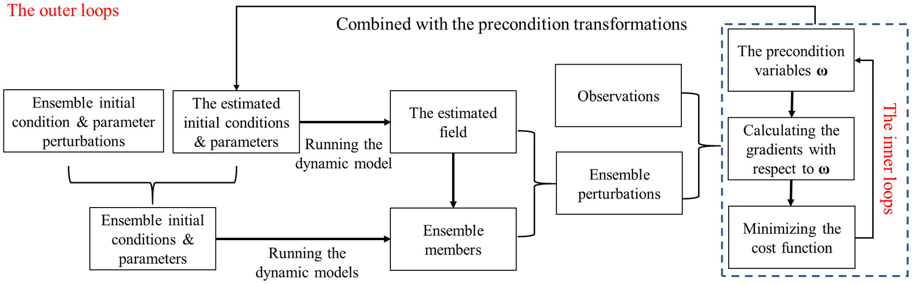
Figure 1 The flowchart of the operational improved analytical four-dimensional ensemble variational (A-4DEnVar).
In the outer loops, the ensemble perturbations are generated based on the μB (and/or μC), and then, they are added to the approximation state variables to obtain the initial conditions or parameters of the ensemble members. The ensemble initial field and parameters are reconstructed in the outer loops of each cycle. The main computational costs for the integrations of ensemble members are only needed in the outer loops, whereas the inner loops focus on the iteration of precondition state variables.
2.3. The independent point scheme
The basic assumption of IP scheme is that the features or characters of the variables to be optimized (such as spatially distributed BFCs) can be determined by the variables located at some key points (Wang et al., 2021). In data assimilation, only these key variables are optimized directly, whereas other general variables are optimized by using interpolation methods (such as Cressman method and uniform or nonuniform spline interpolation methods) based on these key variables. The IP scheme restricts estimation problems from the variable space to the IP space. In practice, the key points are often chosen to be far away from each other so that they are considered to be independent. The background error covariance in the IP space is thus simplified as a diagonal matrix. Meanwhile, the interpolation coefficients are determined by the distances between points; hence, the adjacent points have similar values, obviously. It can be seen that the IP scheme not only reduces the dimension complexity but also introduces an implicit localization in data assimilation schemes.
If the Cressman method (Cressman, 1959) is adopted, it can be described as
where Fg denotes the variable located at a general point, Fi is the variable located at a key point and/or IP, and Wgi is the Cressman coefficient that is determined by the distance between the general point and the IP i.e., dgi, and a predefined parameter R.
3. The numerical model
3.1. Governing equations of forward model
Here, the external mode of the Princeton Ocean Model (POM, Blumberg and Mellor, 1987) is used to simulate tides and tidal currents. The attributes of the POM model include the sigma-coordinate system, curvilinear orthogonal coordinates with an Arakawa C differencing scheme in the horizontal grid, explicit horizontal time differencing, and implicit vertical time differencing. The free surface and split time step method is adopted in which the two-dimensional external mode uses a short time step for a high-accuracy surface simulation and the three-dimensional internal mode uses a long-time step to reduce the computational cost. Based on the framework of POM, the POMgcs is extended to a mixed coordinate system to make the z-coordinate and sigma-coordinate compatible.
After the variables are integrated in the original three-dimensional model from the bottom to the top, the governing equations in the external mode (in z-coordinate) for BFC estimation is
where is a Hamilton operator in the horizontal directions. The meanings of other symbols are listed in Table 1.
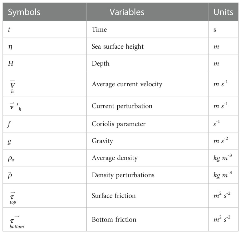
Table 1 The symbols in the external mode of the Princeton Ocean Model with the generalized coordinate system.
The bottom friction is calculated by
where Cd is the BFCs to be optimized.
3.2. Model setting
The model domain is the Bohai and Yellow seas, which covers from 35°N to 41°N in latitudes and 117.5°E to 127.25°E in longitudes. The gridded topography is interpolated from the ETOPO5 datasets. It is shown (in Figure 2) that the depths are all less than 85 m, such that the tide is a basic and major motion in this area. The spatial resolutions are all 1/12° in the east and north directions. In POMgcs, the integration time step is 4 s, which is much enough to simulate the M2 constituent.
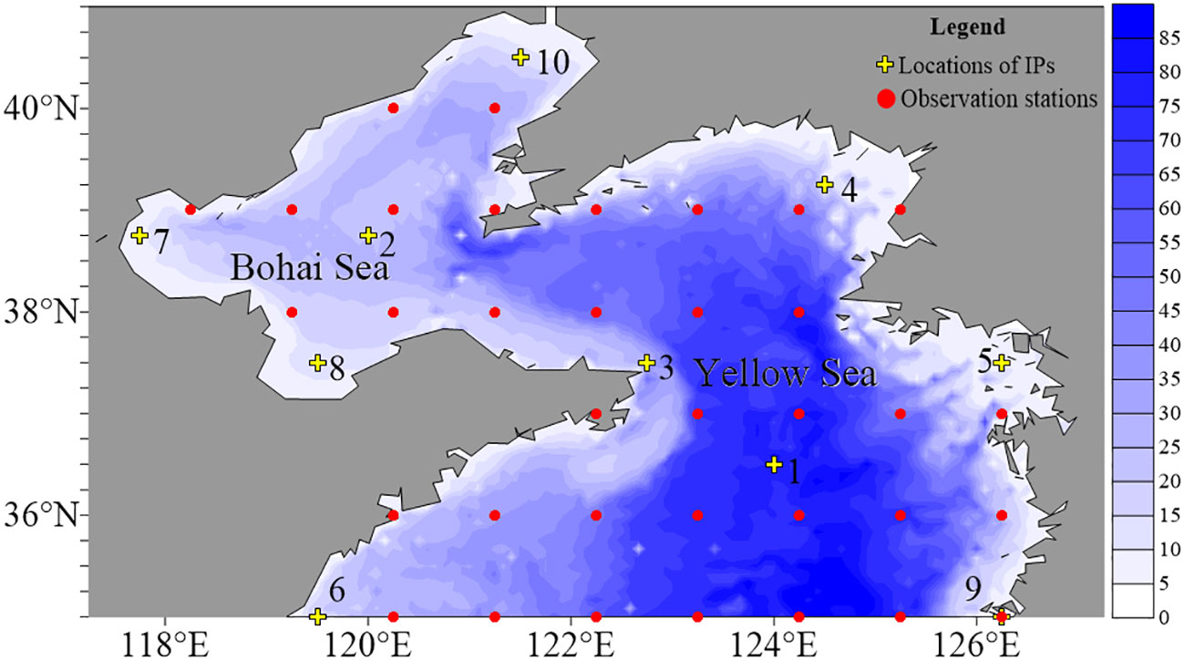
Figure 2 The locations of independent points (IPs; marked with yellow crosses) and the observation stations in EXP 1 to EXP 5 (marked with red dots) for bottom friction coefficient (BFC) optimization.
A static initial condition with zero sea surface height and current velocity is used to spin up the model. Due to the fact that the external mode of POMgcs (a shallow water model) is adopted, the temperature and salinity in initial and open-boundary conditions are constant. The open-boundary conditions including the tide (sea-level height evolution) and tidal currents. Both of them are fixed in the BFC optimization experiments. The open-boundary tide sea-level heights are calculated through the tidal harmonic constants from the same datasets that used to generate the observations, i.e., the NAO datasets. However, because the NAO datasets do not provide the harmonic constants of tidal currents, we have to generate tidal currents from the harmonic constants of TPXO7 (Egbert and Erofeeva, 2002) datasets. To eliminate the misfits of tide and tidal currents, we assimilated the same observations with a fixed-background BFC (that is 0.0025 as used in below experiments) value to provide the optimized open-boundary tidal currents before the inversion of BFCs. The data assimilation method we used is also the operational improved A-4DEnVar. The fixed value is consistent with or close to what was used in other studies. In Yao et al. (2012), the open-boundary conditions of the M2 tidal constituent in the Bohai and the Yellow seas are optimized with the BFCs 0.003. Fan et al. (2019) demonstrated that the value of BFCs in the East China Shelf Seas varies from 0.001 to 0.003. Wang et al. (2021) set the initial BFCs to 0.002 in their experiments. Following these studies, we think that 0.0025 is a reasonable and acceptable value in our study. Moreover, the forcing terms from the sea surface such as wind stress, sensible and/or latent heat flux, and precipitation are not included. The Coriolis parameter takes the local value. The model ran from the 1st to the 7th of January in 2000 in which the first 6 days were used to spin up. All observations are the sea-level heights of the M2 tidal constituent. After that, data assimilation based on A-4DenVar is implemented.
3.3. The locations of IPs and observation stations
The factors that influence the BFC coefficients include topography, water depth, and sediments. Regardless of the attributes of these factors in detail, the distributions of BFCs ought to be continuous and smooth in most regions. The trends and/or characters of the distributions are able to be described through several control points (namely, IPs mentioned above) as indicated in studies. We followed these studies and conducted a twin experiment (denoted as EXP 1) with 10 IPs and a suite of practical experiments (denoted as EXP 2 to EXP 5) with 1, 4, 7, and 10 IPs, respectively. With 10 IPs, we also tested the impacts of observations on the data assimilation performances (EXP 1 and 5). In the last suite of experiments (EXP 6 and EXP 7), density IP stations evenly distributed on an 1°×1° grids are used so that smaller Cressman parameters would be acceptable.
As the main purpose of this paper is to show an operational implementation for A-4DEnVar, we do not discuss how to design a very strict optimal solution for IP locations. Empirically, the selection principle of IPs is that they should be distributed evenly and cover the entire simulation area as much as possible. In EXP 1 to EXP 5, the locations of these points are artificial and presented in Figure 2 (marked with yellow crosses). The observations are calculated from either a twin model (in EXP 1) or the tidal constants of the NAO model (in EXP 2 to EXP 5). The observations are located on stations that gradually increase from 1°×1° (for both the EXP 1 and EXP 2), 1/2°×1/2°,1/4°×1/4° and 1/12°×1/12° in EXP 1 and 5 (the station locations are not shown here). In EXP 6 and EXP 7, the observational stations are only on the 1/12°×1/12° grids. Furthermore, at each station, the simulated observation lasts for 1 day at a frequency of 1 h. The Cressman parameter is set to 5° and fixed so that the whole simulation domain is covered even with only one IP in EXP 1 to EXP 5, whereas it is set to be 2.5° and 1.5° in EXP 6 and EXP 7, respectively.
4. Numerical experiments
4.1. The twin experiments (EXP 1)
The twin experiments are conducted to evaluate the feasibility of A-4DEnVar, and the implementations are expressed in the following steps. First, a suite of random values varying from 1×10⁻⁴ to 3 × 10⁻³ are assigned to the BFCs of the 10 IPs. Second, with these values, the BFCs of the general locations are calculated by the Cressman interpolation method. Starting from the static initial condition and open- boundary conditions mentioned in the above sections, the external mode is integrated for 7 days. In the last 24 h, observations without noise are provided from the simulated “true” sea-level heights at the observation stations. Finally, the operational improved A-4DEnVar is implemented for data assimilation.
Due to the fact that the perfect observations are assimilated in the twin experiment, the optimizations should trust the observations as much as possible. To this end, the algorithm starts from an initial iteration BFC value that is 0.0025 and the background error covariance terms of the cost function are not included. The ensemble size is set to be 10, which is equal to the dimension of state variables, and the factor μ is fixed to 10-6. The stopping criteria for inner loops in each outer loop is important to ensure the coverages of the algorithm. However, the ensemble members and hence the value of tangent linear models and the adjoint models are only updated in the outer loop; it is not necessary to achieve a very exact global minimum in every inner loop where the value of the adjoint models are fixed. Given the balance between effectiveness and the computational cost, empirically, it is convenient to limit the inner loops less than five times in this paper. The outer loop iterations are terminated once the value of the cost function does not decrease significantly.
Figure 3 shows the changes of the cost function value with inner iterations when 1°×1° observational grids are employed. Here, the zero IPs or the zero iterations mean the result without data assimilation. It is clear that, with the iterations, the value of the cost function decreases continually. The experiment results indicate that the model after data assimilation is indeed restrained by the observations. With only one outer loop containing five inner loops, the cost function decreases by more than 77% of the initial cost function value. After 10 iterations, the algorithm converges to a local minimum of the cost function. At the end of the iterations, the cost function value is only 1.2% of the initial cost function value and is much close to zero. However, because the influences of BFCs to the evolutions of sea-level heights are complicated, it is hard to achieve the global minimum for any gradient-based optimization algorithm.
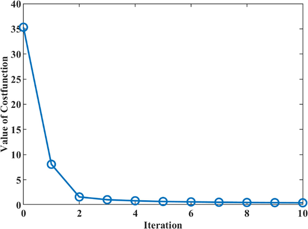
Figure 3 The cost function value decreases with iterations in the twin experiment with perfect observations on the 1°×1° grids.
The distributions of the BFCs are presented in Figure 4 of which Figure 4A is the truth, Figures 4B to E are the experiment results with increasing observational grids, i.e., 1°×1°, 1/2°×1/2°, 1/4°×1/4° and 1/12°×1/12°, respectively, and Figure 4F shows the difference between the results in Figures 4E and 4A. These patterns from EXP 1 are much similar with each other and the experiment result performance is slightly better with the increases of observations. With either sparse or density observations, the proposed algorithm converges to a local minimum of the cost function. Compared with the true BFCs, all the absolute values of these misfits are under 4.5×10⁻⁴ which is much less than the values of BFCs. Specifically, in most areas, the BFC values from experiment results are very close to the truth but are larger in the west of the Yellow seas, near the open boundary, and are smaller in the north of Bohai seas.
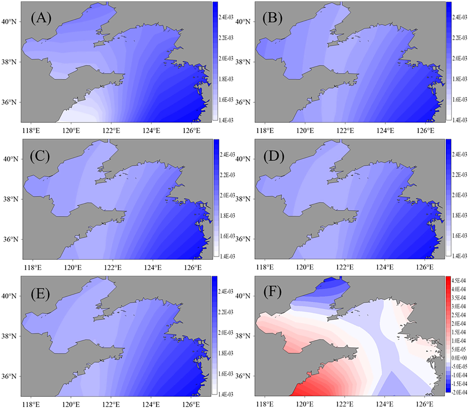
Figure 4 Distributions of the true BFCs (A) and that of experiment results with the 1°×1° (B), 1/2°×1/2° (C), 1/4°×1/4° (D), and 1/12°×1/12° (E) observational grids. (F)is the difference between (E) and (A).
4.2. The practical experiments with different IPs (EXP 2 to EXP 5)
As mentioned above, we designed four experiments (denoted as EXP 2 to EXP 5) with 1, 4, 7, and 10 IPs, respectively, to estimate the BFCs in Bohai and Yellow seas. The settings of practical experiments are similar to that of the twin experiment except for the number of IPs and the generation of observations. The locations of these IPs are the same as what was mentioned in the twin experiments, whereas the observations are calculated from the harmonic constants of the M2 tidal constituent derived from the NAO tide model dataset on their corresponding observation stations.
A great difference between the twin experiment and the practical experiments is that not only the uncertainty from BFCs but also that from other model parameters should be considered simultaneously. However, how to distinguish these uncertainties is complex and beyond the scope of this paper. Instead of discussing them in detail, we assume that these uncertainties are reflected through the observations and the observational errors are Gaussian white noise with a standard deviation of 0.1 m. In the cost function, the background values of BFCs are 0.0025 with a standard deviation of 0.001 (dimensionless). The iteration processes in the practical experiments are set to be the same with that in the twin experiments.
For the experiment with 1°×1° observational grids, Figure 5A shows the impact of the number of IPs on the converged cost function values in EXP 2 to EXP 5. What should be mentioned is that, influenced by other uncertainties in the dynamic model, the cost function values at the beginning and the end of the iterations are both larger than that in the twin experiments. The cost function value decreases by approximately 14% when only one IP is used. The trend that the minimum values of the cost function obtained by A-4DEnVar decreases with the increase of the IPs indicates that the distributions of BFCs are better described with more IPs. When the number of IPs is 7 (in EXP 4), the optimization effect tends to be stable. After that, increasing the number of IPs would not significantly improve the performance. Figure 5B presents the cost function values changes with iterations while 10 IPs are used. Like what we see in the twin experiment, the cost function values also decrease rapidly. In the first five inner iterations, the algorithm almost converges with the fixed ensemble members. After that, once the ensemble members are updated in the outer loop, cost function values decrease a rather big step and then converges again in the inner loops. When 10 inner iterations are implemented, cost function values decrease by approximately 29.6%.
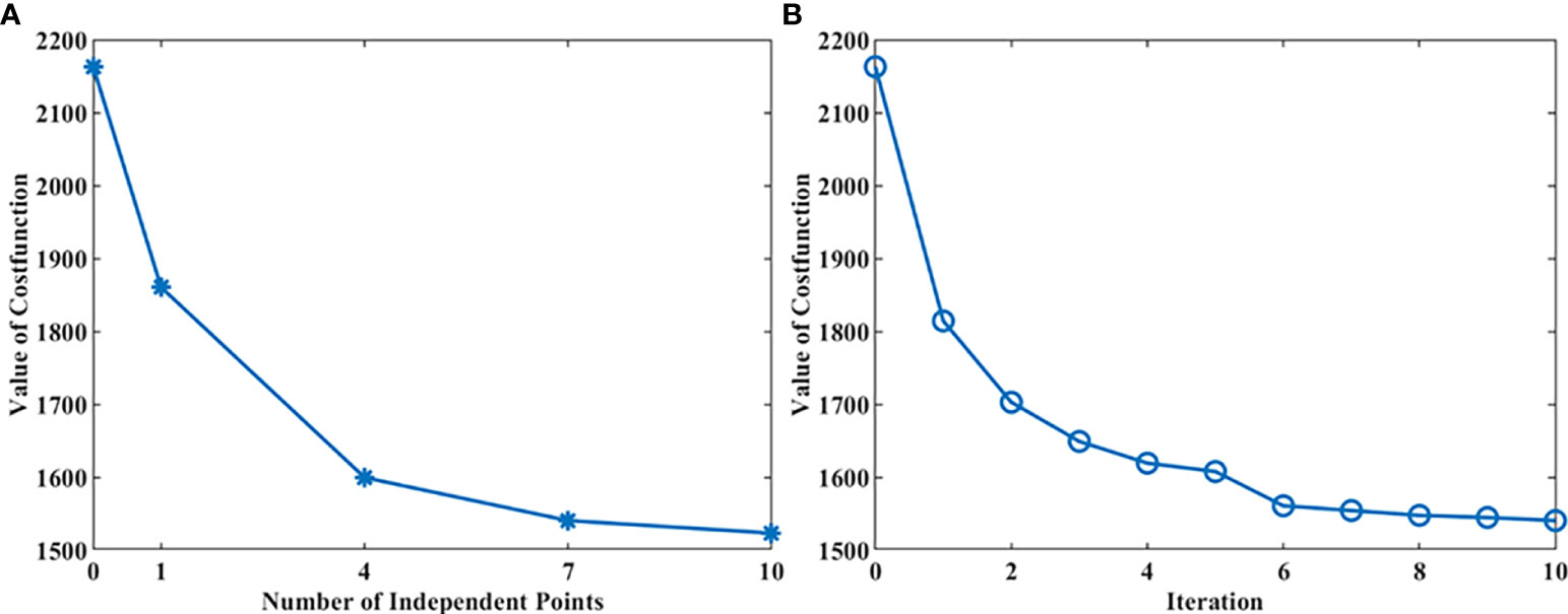
Figure 5 The left (A) shows the impact of the number of IPs on the cost function values when EXP 2 to EXP 5 converged. The right (B) shows the impact of the iterations on the cost function values when 10 IPs are used in EXP. 4.
The amplitudes and phases of M2 tidal constituents are also calculated by the harmonic analysis process. In Figure 6, the cotidal chart from the study of Wang et al. (2021, Figure 6A) and the NAO dataset (Figure 6B) are shown, respectively. Compared to them, it is clear that three amphidromic points in the simulated area and the results we obtained are consistent with those from other studies.
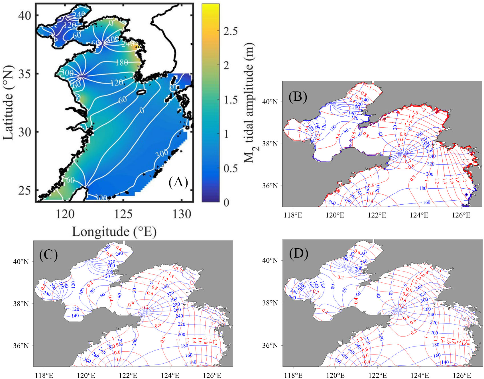
Figure 6 (A, B) are the cotidal charts from Wang et al. (2021) and the National Astronomical Observatory (NAO) data, respectively. (C, D) are the cotidal charts before and after data assimilation.
The cotidal chart differences between the control model results (“CTL” in figures) before data assimilation and that from the NAO model are shown in Figure 7A (for the amplitudes denoted as “H”) and (B) (for the phases denoted as “g”). Figures 7C, D are similar with those in Figures 7A, B but for the results after data assimilation (“DA” in figures). Comparing Figures 7A with C, it is shown that the amplitudes in the north of the Yellow Sea and the middle of the Bohai Sea are much improved. For the phases, great improvements are presented in the north of the Yellow seas around the amphidromic point near (123.5°E, 37.5°N) and the middle of the Bohai Sea. The misfits around (120°E, 40°N) in the north of the Bohai Sea are caused by the different locations of the amphidromic points from the results after data assimilation and NAO datasets. Considering the amplitudes in these areas are almost zeros, although the phases are not close enough to that from the NAO datasets, the sea-level evolutions are, in fact, much closer.
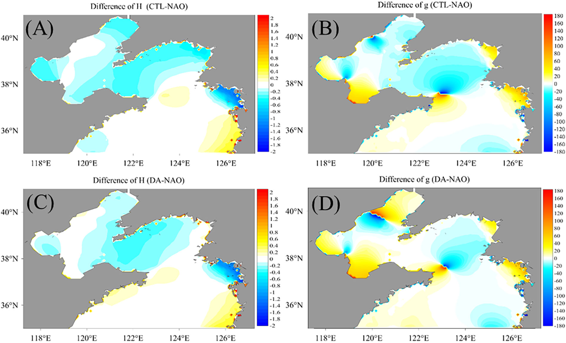
Figure 7 (A, B) are the differences of amplitudes and phases between the control model and NAO datasets, respectively. (C, D) are similar with (A, B) but for the differences between data assimilation results and NAO datasets.
Specifically, Figure 8 shows the data assimilation results in EXP 5 with 10 IPs and different observation densities. Again, consistent with the results in the twin experiment in the above subsections, the patterns are much similar with each other.
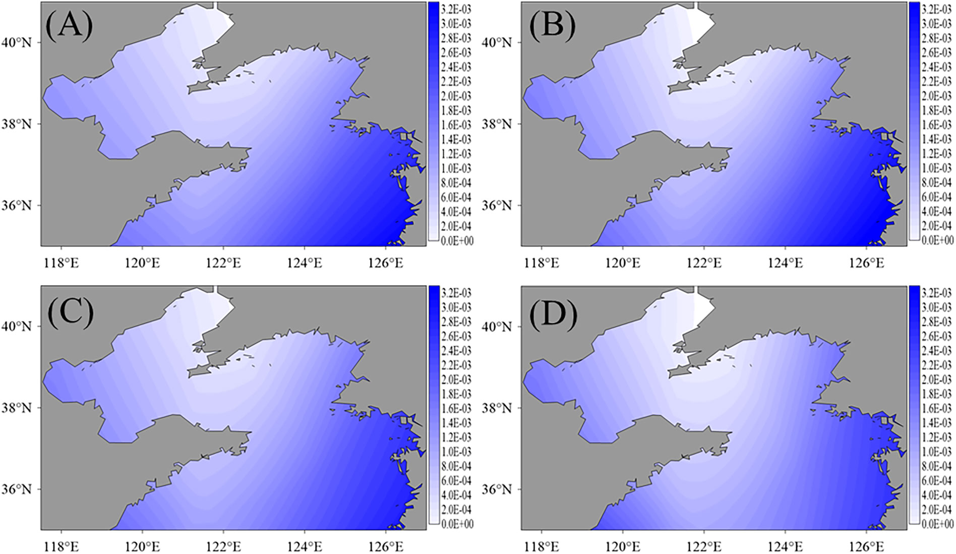
Figure 8 The BFC values after data assimilation from EXP 2 (A), EXP 3 (B), EXP 4 (C) and EXP 5 (D) with different observational grids.
The distributions of BFCs obtained here are much smooth. This is mainly because only 10 IPs and a larger Cressman interpolation parameter are used. For the experiment result in Figure 8A, for example, the average BFC value in the simulation areas is 1.323×10⁻³ and the maximum and minimum values are 3.179×10⁻³ and 9.276×10⁻⁵, respectively. For the same longitude, the values of BFCs in the north are less, and, for the same latitude, the values near the middle of the area are less than that in the east or west areas.
4.3. The practical experiments with different Cressman parameters (EXP 6 and EXP 7)
The last suite of experiments consists of EXP 6 and EXP 7. For both of them, 35 IPs and the 1/12°×1/12° observational grids are used. The optimization processes for them are the same as those in the above subsections. The only differences between them are the Cressman parameters, which are 2.5° and 1.5° in EXP 6 and EXP 7 as mentioned in subsection 3.3.
The experiment results are shown in Figure 9. A larger Cressman parameter might introduce some compensations within the BFC values of IPs. Thus, in the above subsections, the patterns are smoother and the optimization process is more stable than what we obtained here, and, in Figure 9, the pattern from EXP 6 is smoother than that from EXP 7. In Figure 9A, the minimum values of BFCs are located near (37°N, 123°E) in the Yellow seas and the north of the Bohai seas. The maximum values are approximately 5.487×10⁻³ and distributed along the east shores in the Yellow seas. In Figure 9B, with a smaller Cressman parameter, the distribution of the BFCs shows more local features and details. The maximum values are also distributed along the east shores in the Yellow seas, whereas the minimum values appear at (37°N, 123°E).
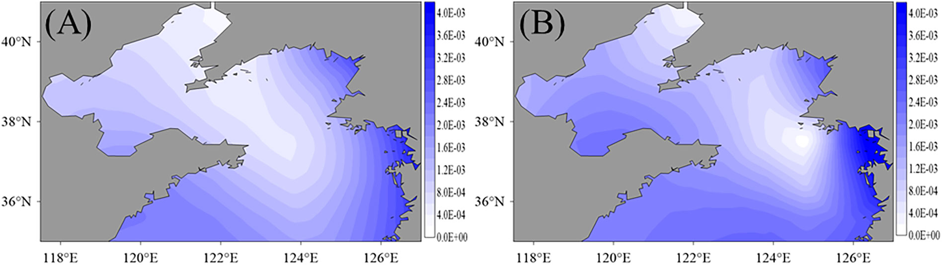
Figure 9 The BFC distributions after data assimilation with the same 35 IPs, 1/12°×1/12° observational grids but with Cressman parameter 2.5° (A) in EXP 6 and 1.5° (B) EXP 7.
A straight intuitive comparison of the data assimilation results is provided through the cotidal charts from EXP 6 and EXP 7 in Figures 10A, B. The differences between the NAO dataset and EXP 6 [amplitudes in (Figure 10C) and phase in (Figure 10D)] are also presented. Compared to Figures 7A, C, it is clear that the differences of amplitudes are further decreased in the Bohai seas and the north of the Yellow seas. A slight increase occurs in the west of the Yellow seas. The differences of phases are not changed significantly here.
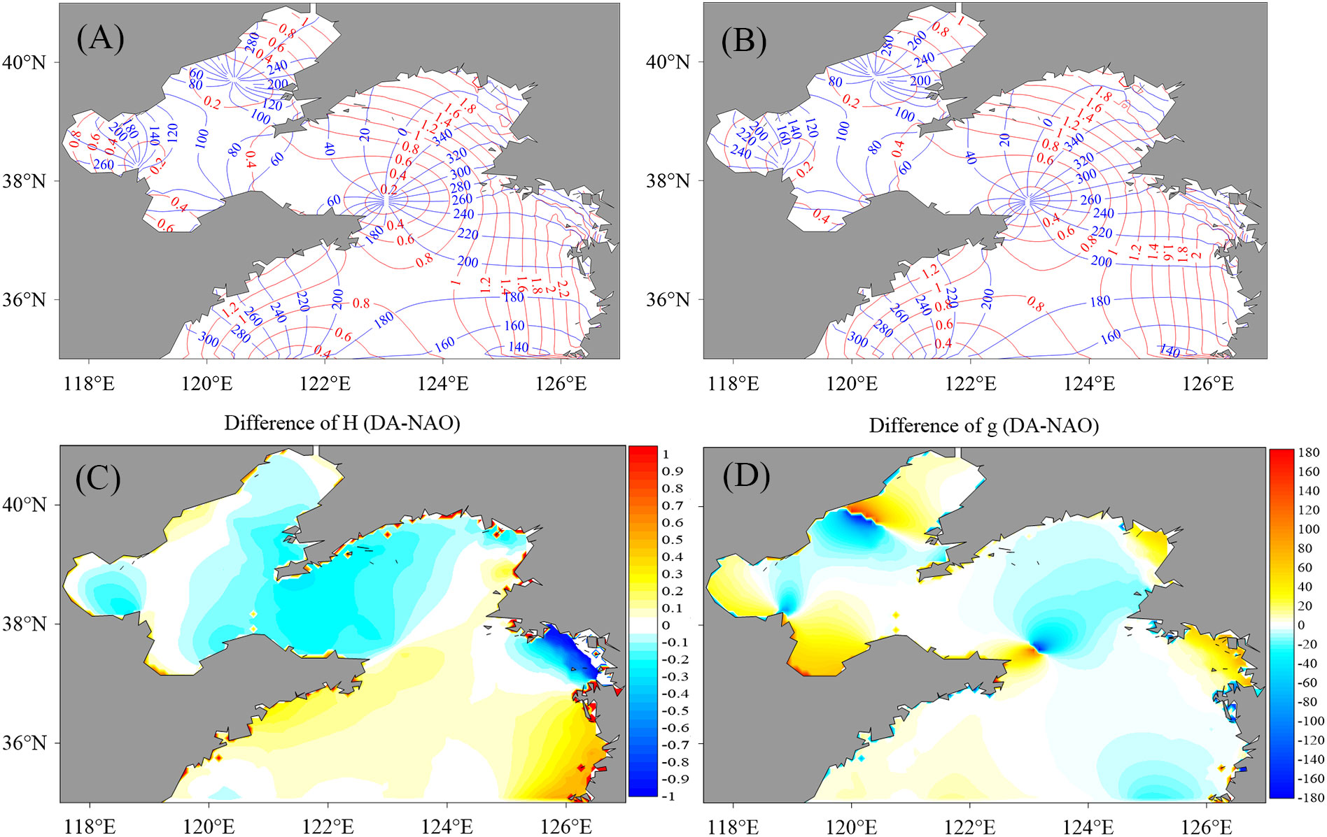
Figure 10 The cotidal chart from EXP 6 (A) and EXP 7 (B) and the differences between EXP 6 and NAO for amplitudes (C) and phases (D).
How to choose the best Cressman parameter is a complex issue to be discussed. The basic principle is to ensure that the interpolation result can cover the full simulation domain. Furthermore, if the stability of data assimilation processes can be guaranteed, one should choose the parameter so that the cost function convergences to a lower value. In Lu and Zhang (2006), the Cressman parameter is set to 2° for a 1° IP grid. In this paper, the cotidal charts from EXP 6 and EXP 7 are much similar to each other and the difference between their cost function values after convergences is less than 2% of its initial value. Based on this evidence, we think that both of the two parameters are acceptable. A more objective and accurate approach might be discussed in the future.
5. Summary
A-4DEnVar is one of the most cutting-edge hybrid data assimilation schemes. In early studies, both theoretical and experimental studies based on ideal chaos dynamic models have shown its equivalence to the conventional 4D-Var and avoided the adjoint models. As we all know, there are still several issues to be explored if one wants to apply the theory and algorithm ideas into an operational system.
This paper is a bridge from the theoretical algorithm to practical operational developments. To reduce the computational cost caused by the inverse of the B matrix, precondition variables are introduced. The algorithm is further designed as an outer–inner loop structure. The ensemble members and hence the estimated corresponding adjoint model values in 4D-Var are updated only in the outer loops so that too-frequent updates of the ensemble members are avoided. The inner loops focus on the gradient-based optimization of the precondition variables. The local minimum of the precondition variables is combined to the increments of state variables in outer loops.
The IP scheme is, in fact, an implicit localization method to construct an empirical B matrix. In practice, the values of the IPs are optimized using data assimilation, and the values of other general points are calculated through interpolation methods such as the Cressman method, linear method, and spline interpolation method. Due to the fact that only IPs are explicitly optimized, the IP scheme can reduce the freedom degree and the complicity of the data assimilation process. In the framework of the operational improved A-4DEnVar, the combination of independent schemes makes it possible to restrict the optimization problems on the IP space. Considering that the number of IPs is much less than that of original variables, the ill-posedness is, in fact, limited. Moreover, the IP scheme also introduces an implicit localization that increases the stability of the algorithm.
We constructed the twin experiments and practical experiments to validate the performance of the improvement variant of the A-4DEnVar on the optimization of the BFCs in the Bohai and Yellow seas. In the twin experiment, the perfect observations are used and the cost function decreases rapidly. In the practical experiment, the observations calculated from the tidal harmonic constants of the NAO tide model are used. Compared with the cotidal chart from the original NAO datasets, both the tidal heights and lag phases are improved. After assimilation, the BFCs of the open-sea areas are larger than that of the coastal areas for the same latitude, and, for the same longitude, the BFCs of the Bohai Sea are slightly smaller than that of the Yellow Sea. It is concluded that the operational improved variant of A-4DEnVar works well in the spatially distributed parameter estimation problems.
We demonstrate that, if without the operational improvement, it is a difficult task for the original A-4DEnVar to optimize the BFCs in such vast areas. On the one hand, to construct a full-rank background error covariance and ensure a proper estimation of the adjoint model, the original A-4DEnVar has to generate more than 4,000 (which is the number of BFCs in the POMgcs model) ensemble members. It is clear that the burden of computation cost is too high if the IP scheme is not considered. On the other hand, the local correlations of these BFCs are hard to construct if the Cressman interpolation (or other interpolation skill) method is not considered. It would be a trouble to calculate the inverse of such a big background error covariance matrix, too. In summary, although better improvements might be proposed for A-4DEnVar in the future, in this stage, the IP scheme is necessary and cannot be replaced or ignored in the experiments.
In addition to the issues above, there are some points that are beyond the scope of this paper, but they should be studied in our future studies. On the one hand, this paper explores the performance of A-4DEnVar on the parameter estimation with an implicit localization method, but the proposed algorithm should be widely validated in the initial condition field estimation with large freedom degrees. On the other hand, only the M2 tide constituent is mentioned in this paper. However, many tidal constituents are combined with each other in the real world. It is worthwhile to apply the improved scheme to the inversion of BFCs under a more realistic model.
Data availability statement
The original contributions presented in the study are included in the article/Supplementary Material. Further inquiries can be directed to the corresponding author.
Author contributions
KL and WL had the conceptualization and methodology; GH and XW validated the result; KL wrote the manuscript and WL, GH, XW, and XQ reviewed it. All authors have read and agreed to the published version of the manuscript.
Funding
This research was funded by grants from the National Key Research and Development Program (2022YFC3104804 and 2021YFC3101501) and the National Natural Science Foundation (41876014) of China.
Acknowledgments
The authors acknowledge valuable discussions with Hanyu Liu, Song Hu, and Ru Wang from the School of Marine Science and Technology of Tianjin University.
Conflict of interest
The authors declare that the research was conducted in the absence of any commercial or financial relationships that could be construed as a potential conflict of interest.
Publisher’s note
All claims expressed in this article are solely those of the authors and do not necessarily represent those of their affiliated organizations, or those of the publisher, the editors and the reviewers. Any product that may be evaluated in this article, or claim that may be made by its manufacturer, is not guaranteed or endorsed by the publisher.
References
Blumberg A. F., Mellor G. L. (1987). “A description of a three-dimensional coastal ocean circulation model,” in Three-dimensional coastal ocean models, coastal estuarine studies 4. Ed. Heaps N. S. (Washington: American Geophysical Union), 1–16.
Buehner M. (2005). Ensemble-derived stationary and flow-dependent background-error covariances: Evaluation in a quasi-operational NWP setting. Q.J.R. Meteorol. Soc 131 (607), 1013–1043. doi: 10.1256/qj.04.15
Buehner M., Houtekamer P. L., Charette C., Mitchell H. L., He B. (2010a). Intercomparison of variational data assimilation and the ensemble kalman filter for global deterministic NWP. part I: Description and single-observation experiments. Mon. Wea. Rev. 138 (5), 1550–1566. doi: 10.1175/2009MWR3157.1
Buehner M., Houtekamer P. L., Charette C., Mitchell H. L., He B. (2010b). Intercomparison of variational data assimilation and the ensemble kalman filter for global deterministic NWP. part II: One-month experiments with real observations. Mon. Wea. Rev. 138 (5), 1567–1586. doi: 10.1175/2009MWR3158.1
Courtier P., Talagrand O. (1987). Variational assimilation of meteorological observations with the adjoint vorticity equation II: Numerical results. Q.J.R. Meteorol. Soc 113, 1329–1347. doi: 10.1002/qj.49711347813
Cressman G. P. (1959). An operational objective analysis system. Monthly Weather Rev. 87, 10, 367–374. doi: 10.1175/1520-0493(1959)087<0367:AOOAS>2.0.CO;2
Egbert G. D., Erofeeva S. Y. (2002). Efficient inverse modeling of barotropic ocean tides. J. Atmospheric Oceanic Technology. 19, 183–204. doi: 10.1175/1520-0426(2002)019<0183:EIMOBO>2.0.CO;2
Evensen G. (1994). Sequential data assimilation with a nonlinear quasi-geostrophic model using Monte-Carlo methods to forecast error statistics. J. Geophys. Res. 99, 10143–10162. doi: 10.1029/94JC00572
Evensen G. (2004). Sampling strategies and square root analysis schemes for the EnKF. Ocean Dynam. 54, 539–560. doi: 10.1007/s10236-004-0099-2
Ezer T., Mellor G. L. (2004). A generalized coordinate ocean model and a comparison of the bottom boundary layer dynamics in terrain-following and in z-level grids. Ocean Modelling. 6 (3-4), 379–403. doi: 10.1016/S1463-5003(03)00026-X
Fan R., Zhao L., Lu Y., Nie H., Wei H. (2019). Impacts of currents and waves on bottom drag coefficient in the East China shelf seas. J. Geophysical Research: Oceans 124 (11), 7344–7354. doi: 10.1029/2019jc015097
Goodliff M., Amezcua J., Van Leeuwen P. J. (2015). Comparing hybrid data assimilation methods on the Lorenz 1963 model with increasing non-linearity. Tellus A 67 (1). doi: 10.3402/tellusa.v67.26928
Guo Z., Pan H. D., Fan W., Lv X. Q. (2017). Application of surface spline interpolation in inversion of bottom friction coefficients. J. Atmos. Ocean. Technol. 34 (9), 2021–2028. doi: 10.1175/JTECH-D-17-0012.1
Kalnay E., Li H., Miyoshi T., Yang S. C., Ballabrera J. (2007). 4D-var or ensemble kalman filter? Tellus A. 59 (5), 758–773. doi: 10.1111/j.1600-0870.2007.00261.x
Liang K., Li W., Han G., Shao Q., Zhang X., Zhang L., et al. (2021). An analytical four-dimensional ensemble-variational data assimilation scheme. J. Adv. Modeling Earth Syst. 13, e2020MS002314. doi: 10.1029/2020MS002314
Liu C., Xiao Q. (2013). An ensemble-based four-dimensional variational data assimilation scheme. part III: Antarctic applications with advanced research WRF using real data. Mon. Wea. Rev. 141 (8), 2721–2739. doi: 10.1175/MWR-D-12-00130.1
Liu C., Xiao Q., Wang B. (2008). An ensemble-based four-dimensional variational data assimilation scheme. part I: Technical formulation and preliminary test. Mon. Wea. Rev. 136 (9), 3363–3373. doi: 10.1175/2008MWR2312.1
Liu C., Xiao Q., Wang B. (2009). An ensemble-based four-dimensional variational data assimilation scheme. part II: Observing system simulation experiments with advanced research WRF (ARW). Mon. Wea. Rev. 137 (5), 1687–1704. doi: 10.1175/2008MWR2699.1
Liu C. S., Xue M. (2016). Relationships among four-dimensional hybrid ensemble-variational data assimilation algorithms with full and approximate ensemble covariance localization. Mon. Wea. Rev. 144, 591–606. doi: 10.1175/MWR-D-15-0203.1
Lorenc A. C., Bowler N. E., Clayton A. M., Pring S. R., Fairbairn D. (2015). Comparison of hybrid-4DEnVar and hybrid-4DVar data assimilation methods for global NWP. Mon. Wea. Rev. 143 (1), 212–229. doi: 10.1175/MWR-D-14-00195.1
Lu X. Q., Zhang J. C. (2006). Numerical study on spatially varying bottom friction coefficient of a 2D tidal model with adjoint method. Continental Shelf Res. 26 1905–1923. doi: 10.1016/j.csr.2006.06.007
Matsumoto K., Takanezawa T., Ooe M. (2000). Ocean tide models developed by assimilating TOPEX/POSEIDON altimeter data into hydrodynamical model: A global model and a regional model around Japan. J. Oceanography. 56, 567–581. doi: 10.1023/A:1011157212596
Oddo P., Storto A., Dobricic S., Russo A., Lewis C., Onken R., et al. (2016). A hybrid variational-ensemble data assimilation scheme with systematic error correction for limited-area ocean models. Ocean Sci. 12 (5), 1137–1153. doi: 10.5194/os-12-1137-2016
Pan H., Guo Z., Lv X. (2017). Inversion of Tidal Open Boundary Conditions of the M2 Constituent in the Bohai and Yellow Seas. J. Atmospheric and Oceanic Tech. 34 1661–1672. doi: 10.1175/JTECHD-16-0238.1
Qian S. H., Wang D. S., Zhang J. C., Li C. Y. (2021). Adjoint estimation and interpretation of spatially varying bottom friction coefficients of the M2 tide for a tidal model in the bohai, yellow and East China seas with multi-mission satellite observations. Ocean Modelling. 161. doi: 10.1016/j.ocemod.2021.101783
Rabier F., Järvinen H., Klinker E., Mahfouf J.-F., Simmons A. (2000). The ECMWF operational implementation of four-dimensional variational assimilation. I: Experimental results with simplified physics. Q.J.R. Meteorol. Soc 126, 1143–1170. doi: 10.1002/qj.49712656415
Rawlins F., Ballard S. P., Bovis K. J., Clayton A. M., Li D., Inverarity G. W., et al. (2007). The met office global four-dimensional variational data assimilation scheme. Q.J.R. Meteorol. Soc 133, 347–362. doi: 10.1002/qj.32
Stammer D., Wunsch C., Giering R., Eckert C., Heimbach P., Marotzke J., et al. (2002). Global ocean circulation during 1992–1997, estimated from ocean observations and a general circulation model. J. Geophys. Res. 107 (C9), 3118. doi: 10.1029/2001JC000888
Storto A., Oddo P., Cipollone A., Mirouze I., Lemieux B. (2018). Extending an oceanographic variational scheme to allow for affordable hybrid and four-dimensional data assimilation. Ocean Modelling. 128, 67–86. doi: 10.1016/j.ocemod.2018.06.005
Talagrand O., Courtier P. (1987). Variational assimilation of meteorological observations with the adjoint vorticity equation. I: Theory. Q.J.R. Meteorol. Soc 113, 1311–1328. doi: 10.1002/qj.49711347812
Tian X., Han R., Zhang H. (2020). An adjoint-free alternating direction method for four-dimensional variational data assimilation with multiple parameter tikhonov regularization. Earth Space Sci. 7, e2020EA001307. doi: 10.1029/2020EA001307
Tian X., Zhang H. (2019a). A big data-driven nonlinear least squares four-dimensional variational data assimilation method: Theoretical formulation and conceptual evaluation. Earth Space Sci. 6, 1771–1774. doi: 10.1029/2019EA000735
Tian X., Zhang H. (2019b). Implementation of a modified adaptive covariance inflation scheme for the big data-driven NLS-4DVar algorithm. Earth Space Sci. 6, 2593–2604. doi: 10.1029/2019EA000963
Tian X., Zhang H., Feng X., Xie Y. F. (2018). Nonlinear least squares En4DVar to 4DEnVar methods for data assimilation: Formulation, analysis, and preliminary evaluation. Mon. Wea. Rev. 146, 77–93. doi: 10.1175/MWR-D-17-0050.1
Wang D., Zhang J., Wang Y. p. (2021). Estimation of bottom friction coefficient in multi-constituent tidal models using the adjoint method: Temporal variations and spatial distributions. J. Geophysical Res. Oceans 126, e2020JC016949. doi: 10.1029/2020JC016949
Wunsch C., Heimbach P. (2013). Dynamically and kinematically consistent global ocean circulation and ice state estimates. Int. Geophysics 103, 553–579. doi: 10.1016/B978-0-12-391851-2.00021-0
Yao Z., He R., Bao X., Wu D. X., Song J. (2012). M2 tidal dynamics in bohai and yellow seas: a hybrid data assimilative modeling study. Ocean Dynamics 62, 753–769. doi: 10.1007/s10236-011-0517-1
Zhang J. C., Lu X. Q. (2008). Parameter estimation for a three-dimensional numerical barotropic tidal model with adjoint method. Int. J. Numer. Methods Fluids 57, 47–92. doi: 10.1002/fld.1620
Zhang J. C., Lu X. Q. (2010). Inversion of three-dimensional tidal currents in marginal seas by assimilating satellite altimetry. Comput. Methods Appl. Mech. Eng. 199, 3125–3136. doi: 10.1016/j.cma.2010.06.014
Zhang J. C., Lu X. Q., Wang P., Wang Y. P. (2011). Study on linear and nonlinear bottom friction parameterizations for regional tidal models using data assimilation. Continental Shelf Res. 31, 6, 555–573. doi: 10.1016/j.csr.2010.12.011
Zhang H., Tian X. (2018). A multigrid nonlinear least squares four-dimensional variational data assimilation scheme with the advanced research weather research and forecasting model. J. Geophys. Res. Atmos. 123, 5116–5129. doi: 10.1029/2017JD027529
Keywords: A-4DEnVar, hybrid, bottom friction coefficients, Bohai and Yellow Seas, localization
Citation: Liang K, Li W, Han G, Wang X and Qiu X (2023) An operational improvement of A-4DEnVar and its application to the estimation of the spatially varying bottom friction coefficients of the M2 constituent in the Bohai and Yellow seas. Front. Mar. Sci. 9:1084159. doi: 10.3389/fmars.2022.1084159
Received: 30 October 2022; Accepted: 19 December 2022;
Published: 13 January 2023.
Edited by:
Yasumasa Miyazawa, Japan Agency for Marine-Earth Science and Technology (JAMSTEC), JapanReviewed by:
Jicai Zhang, Zhejiang University, ChinaShuhei Masuda, Japan Agency for Marine-Earth Science and Technology (JAMSTEC), Japan
Copyright © 2023 Liang, Li, Han, Wang and Qiu. This is an open-access article distributed under the terms of the Creative Commons Attribution License (CC BY). The use, distribution or reproduction in other forums is permitted, provided the original author(s) and the copyright owner(s) are credited and that the original publication in this journal is cited, in accordance with accepted academic practice. No use, distribution or reproduction is permitted which does not comply with these terms.
*Correspondence: Wei Li, bGl3ZWkxOTc4QHRqdS5lZHUuY24=; Guijun Han, Z3VpanVuX2hhbkB0anUuZWR1LmNu