 Fuad Azminuddin
 Chan Joo Jang
 Dongchull Jeon2
- 1Department of Oceanography, University of Science and Technology, Daejeon, South Korea
- 2Ocean Circulation Research Division, Korea Institute of Ocean Science and Technology, Busan, South Korea
The New Guinea Coastal Undercurrent (NGCUC) is considered a bottleneck in the western tropical Pacific (WTP), carrying upper-to-intermediate waters from the south to the northwestern Pacific, thereby playing a fundamen tal role in the interhemispheric water mass exchange. However, how the NGCUC links to the circulation in the WTP was insufficiently studied. This work explores the destination of NGCUC waters, its spatiotemporal changes, and possible physical processes linked with the downstream NGCUC using ocean reanalysis for 22 years (1994 – 2015). Lagrangian particle tracking discloses eight major destinations of the NGCUC: The Equatorial Undercurrent (EUC, 35.26%), the North Equatorial Countercurrent (NECC, 12.3%), the North (13.33%) and South (8.85%) Subsurface Countercurrents, the Equatorial Deep Jet (11.49%), the Mindanao Undercurrent (13.24%), and the Indonesian (3.47%) and Halmahera (0.86%) Throughflows. The NGCUC waters are distributed mainly to the east (81.65%) and their dissemination varies markedly with depth. These destinations exhibit significant variations on seasonal and interannual time scales. The NGCUC strengthens (weakens) during summer (winter) and more NGCUC waters are distributed westward and northeastward (eastward). Interannually, the distribution of the NGCUC water is influenced by El Niño-Southern Oscillation, in which most of its eastward-distributed waters shift northward (equatorward) in El Niño (La Niña) phase joining the strengthened NECC (EUC). Changes in the NGCUC water destination can transform the water mass properties in the WTP. The findings of this study also emphasize the fundamental role of eddies in trapping and redistributing the NGCUC waters and linking the currents in the WTP.
1. Introduction
The western tropical Pacific (WTP) is the home of the largest area of permanent warm water (>28°C) in the world ocean, which is so-called western Pacific warm pool (Hu et al., 2020), and is characterized by the complex ocean circulation including the narrow alternating zonal flows and intense boundary current system, namely the Pacific western boundary currents (WBC) (Hu and Cui, 1991; Hu et al., 2020). The east coast of the Philippines and the north coast of New Guinea Island are two regions in the WTP with prominent boundary currents at both surface and subsurface layers. The Pacific WBC includes the Kuroshio Current (KC), Mindanao Current (MC), and New Guinea Coastal Current (NGCC) at the upper layer, and the Luzon Undercurrent, Mindanao Undercurrent (MUC), and New Guinea Coastal Undercurrent (NGCUC) below the thermocline (see Figure 1).
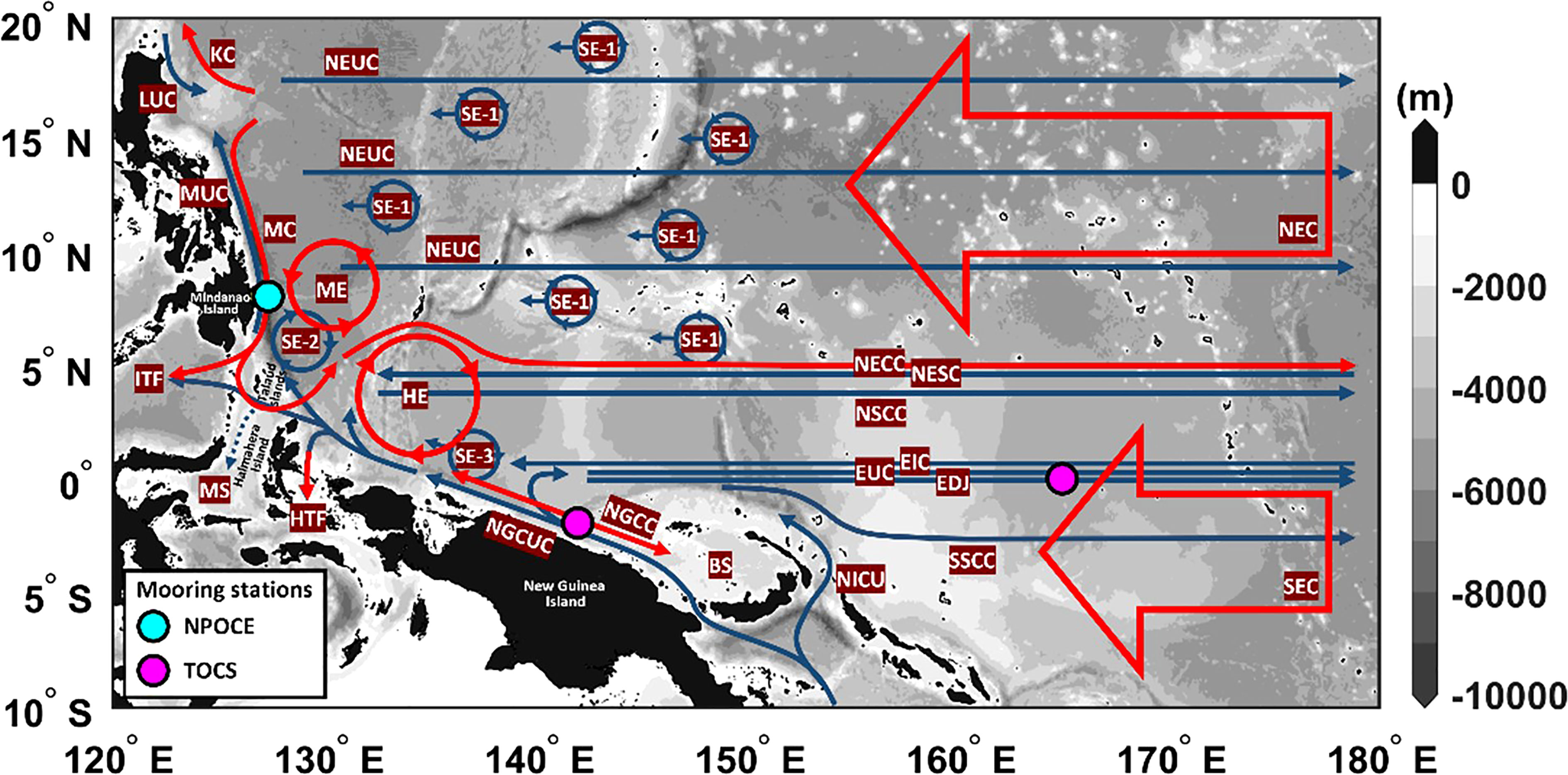
Figure 1 General pattern of the surface (red arrows) and subsurface (blue arrows) currents and eddies in the tropical western Pacific. The surface currents and eddies are the NEC (North Equatorial Current), the KC (Kuroshio Current), the MC (Mindanao Current), the NECC (North Equatorial Countercurrent), the SEC (South Equatorial Current), the NGCC (New Guinea Coastal Current), the ITF (Indonesian Throughflow), HTF (Halmahera Throughflow), the HE (Halmahera Eddy), and the ME (Mindanao Eddy). The subsurface currents and eddies are the NEUC (North Equatorial Undercurrent), the LUC (Luzon Undercurrent), the MUC (Mindanao Undercurrent), the NESC (North Equatorial Subsurface Current), the NSCC (North Subsurface Countercurrent), the EUC (Equatorial Undercurrent), EIC (Equatorial Intermediate Current), EDJ (Equatorial Deep Jets), the NGCUC (New Guinea Coastal Undercurrent), the NICU (New Ireland Coastal Undercurrent), the SE-1 (westward-propagating Subthermocline Eddy), the SE-2 (anticyclonic Subthermocline Eddy southeast of Mindanao Island), and the SE-3 (northwestward-propagating Subthermocline Eddy). The colored circles indicate the ADCPs mooring stations. The color shading indicates bathymetry (m).
The WTP has also rich eddy activity. There are two prominent surface eddies, i.e., Mindanao Eddy (ME) and Halmahera Eddy (HE), in which nonlinearity on a β plane is previously suggested as the possible mechanism responsible for their establishment (Arruda and Nof, 2003). The ME and HE are thought to be quasi-stationary eddies with cyclonic and anticyclonic polarities, respectively, and are located at the retroflection points of the MC and NGCC/NGCUC, respectively, connecting these equatorward WBC with the eastward-flowing North Equatorial Countercurrent (NECC) (Kashino et al., 2013). Below the surface, there are, at least, two groups of subthermocline eddies (SEs): one is originated from the central Pacific and the other is originated from the New Guinea coast (e.g., Chiang and Qu, 2013; Chiang et al., 2015). In addition, a recent study has suggested that there is a distinct anticyclonic SE southeast of Mindanao Island (Azminuddin et al., 2022). Less is known about its characteristics and driving mechanism. While its presence remains uncertain, the establishment of this eddy feature is possibly due to the tilting of HE poleward with increasing depth (Qu et al., 1999; Kashino et al., 2013). In this study, the westward-propagating SEs, the anticyclonic SE southeast of Mindanao Island, and the northwestward-propagating SEs from the New Guinea Coast are then called SE(s)-1, SE-2, and SE(s)-3, respectively (see Figure 1).
It has been largely known that the WTP is a meeting place for intermediate waters. There are the northern, southern, and equatorial Pacific-sourced intermediate waters (Bingham and Lukas, 1994; Max et al., 2016). The NGCUC serves as the primary throughflow that transfers the South Pacific waters, e.g., South Pacific Tropical Water (SPTW) and Antarctic Intermediate Water (AAIW), into the northwestern tropical Pacific through the Vitiaz Strait, crossing the equator near 140°E and influencing the intermediate water properties and heat content in the North Pacific (e.g., Fine et al., 1994; Wang and Hu, 1998; Qu and Lindstrom, 2004; Kawabe et al., 2008; Hu et al., 2015). But the complexity of the current system in the WTP has made it challenging to accurately investigate how the South Pacific waters spread out over the northwestern Pacific.
Studies have confirmed that a large part of water masses carried by NGCUC are transported eastward mainly through Equatorial Undercurrent (EUC) and Northern Subsurface Countercurrent (NSCC), in which the NGCUC splits into some branches at different depths in the region between Mindanao and New Guinea (Wang et al., 2016b; Li et al., 2020; Zhang et al., 2020; Li et al., 2021). The eastward-flowing EUC centered around the equator over a depth range of 100 – 300 m, while NSCC lies just north of EUC and south of 4°N at the deeper layer around the depths of 200 – 600 m (Wang et al., 2016b; Song et al., 2018). In addition, using Lagrangian trajectory computation Wang et al. (2019) suggested that the NGCUC water is also partly distributed into NECC at the shallower depth centered around 100 m.
While most of the NGCUC waters are transferred eastward, some portions are also distributed poleward through MUC. Some studies have made it evident that South Pacific water, i.e., AAIW, exists east of the Mindanao coast (e.g., Qu and Lindstrom, 2004). The NGCUC strengthening, topographic features, and SEs are hypothesized to facilitate their connection (Qu et al., 2012; Wang et al., 2016a). Although the poleward distribution of AAIW through MUC has been widely investigated, to date, the pathway and underlying process of AAIW into MUC have not been properly established presumably owing to a lack of direct measurements in the subsurface. Furthermore, mechanisms responsible for the NGCUC water allocation into several major destinations, i.e., EUC, NSCC, NECC, MUC, etc., and how they change over time have not been researched intensively. In the present study, ocean reanalysis data is analyzed for investigating the fate of NGCUC waters, its spatiotemporal changes, and how the NGCUC links to the currents in the WTP. We also consider the possible impacts of eddies on this circulation system that was previously suggested (e.g., Chiang and Qu, 2013; Wang et al., 2014).
The following sections of this paper are organized as follows: Section 2 briefly describes the data and methods used for the present study. The main results are described in Section 3, which presents the data validations, describes the mean structure of the currents that are possibly connected to the NGCUC, investigates the destination of the NGCUC, their spatiotemporal changes, and explores their implications on the characteristics and transformation of waters in the WTP. Section 4 discusses the potential roles of eddies and the possible currents’ linkages. Section 5 summarizes the outcomes of the present study.
2. Data and methods
2.1. Data
In this study, 22 years (from 1994 to 2015) of velocity data from three widely-used global ocean reanalysis datasets are utilized. They are the daily Global Ocean Reanalysis and Simulation Version 4 (GLORYS2V4) produced by Mercator Ocean (http://marine.copernicus.eu) (Lellouche et al., 2013), 3-daily Oceanic General Circulation Model for the Earth Simulator (OFES) that driven by National Centers for Environmental Prediction winds (http://apdrc.soest.hawaii.edu/las_ofes) (Sasaki et al., 2008), and 3-hourly Hybrid Coordinate Ocean Model (HYCOM) version 2.2.99DH, which is the Global Ocean Forecasting System 3.1, (http://www.hycom.org) (Chassignet et al., 2009). The GLORYS2V4 has a horizontal resolution of 0.25° and 75 vertical layers, with a layer thickness that increases gradually from 1 m near the surface to approximately 200 m in the deep layer. The OFES has a horizontal resolution of 0.1°, 54 vertical layers, and a vertical resolution of 5 m near the surface to approximately 330 m in the deep layer. While the HYCOM has a horizontal resolution of 1/12°, 41 vertical layers, and a vertical resolution of 2 m near the surface to approximately 1,000 m in the deep layer. Detailed descriptions of these models are available in the above respective links and research papers.
Also included in this study are moored acoustic Doppler current profiler (ADCP) datasets from the Northwestern Pacific Ocean Circulation and Climate Experiment (NPOCE) (http://npoce.org.cn/) and the Tropical Ocean Climate Study (TOCS) (http://www.jamstec.go.jp/) programs (see Figure 1) to validate the model outputs. One mooring from NPOCE was deployed at the east of Mindanao Island (8°N, 127.3°E) from 1 December 2010 to 7 December 2012. The moored ADCPs have recorded velocities from the near-surface down to the depth deeper than 1,200 m by using an upward- and a downward-looking 75 kHz ADCPs manufactured by Teledyne RD Instruments (TRDI) that were mounted on the mooring line at about 400 m. More details of this mooring can be found in Zhang et al. (2014). Two moorings, which are provided by TOCS, were deployed at the north of New Guinea Island (2°S, 142°E) from 12 July 1995 to 5 September 1998 and at the equatorial pacific (165°E) from 31 January 1997 to 8 July 2001. Both recorded velocities of upper ~300 m by using upward-looking 150 kHz ADCPs manufactured by TRDI. Detailed information on these two moorings can be obtained in Kuroda (2000) and Kutsuwada and McPhaden (2002), respectively. These three mooring stations were selected to validate the reanalyses and to provide observational evidence for the MUC, NGCUC, and EUC, respectively.
2.2. Methods
2.2.1. Lagrangian particle tracking and experimental design
One possible way to understand the destination of NGCUC is by tracing its water parcels. In the present study, the Lagrangian particle tracking method (LPTM) is applied to track water parcels that originate from the NGCUC region, assuming that the water parcels are passive tracers. Following Seo et al. (2020) but without the wind drift (since subsurface water parcels rather than floating objects at the surface), the trajectories of each tracer can be calculated as follows:
where is the tracer’s position (x,y ) at time t , ∆t is the time interval (daily), is the velocity of ocean current. The last term in (1) is a random walk component to resolve sub-grid scale phenomenon, e.g., submesoscale turbulent flow (North et al., 2006). R is a normally distributed random number between -1 and 1, and Kh is a horizontal diffusion coefficient using the Smagorinsky diffusivity scheme (Smagorinsky, 1963),
where A is an adjustment constant defined as 0.02, and ∆x and ∆y are the grid spacing (Choi et al., 2018).
This method allows us to trace the destination (forward integration) of water parcels from the given initial position. To accurately calculate the travel distance, we applied the Runge-Kutta 4th-order method for time integration (Dormand and Prince, 1980). The particle tracking was calculated by using the output of ocean reanalysis data, which is spatially discretized into a grid structure. To estimate the trajectories of each tracer, the velocities that are closest to the corresponding tracer are interpolated using bilinear interpolation, and then the tracer’s position is updated daily. If a tracer reaches a land grid, it is set to be reflected to the nearest ocean grid since it cannot be beached. The reliability of the LPTM is further discussed in Section 3.1.
Tracing a water parcel below the surface, which consists of horizontal and vertical movements, is rather complicated. Nevertheless, it is much easier to move along isopycnals than across them (diapycnal). Therefore, the water flow typically tends to follow isopycnal layers, although diapycnal advection sometimes occurs due to mixing (Ledwell et al., 1993). To more reliably track the tracers, we applied the LPTM along the potential density (σθ ) surface rather than the depth surface. We selected several isopycnal layers that cover most of the NGCUC’s vertical range and are expected to represent the typical depth of the NGCUC destinations, i.e., 23, 25, 26, 26.75, 27, and 27.2 σθ . Detailed descriptions of these layers will be provided in Section 3.2.
For each isopycnal layer, we released 50 tracers from the NGCUC region (see Figure 2 for the tracers’ initial position). The tracers were released every day from 1994 to 2013 with the travel time of two years, which is limited by computing resources. So, a total of 365,250 tracers were simulated at each layer. Preliminary experiments using GLORYS2V4 suggested that there are eight major destinations of NGCUC. Five destinations are the zonally eastward currents including the EUC, the NECC, the NSCC, the Southern Subsurface Countercurrent (SSCC), and the Equatorial Deep Jet (EDJ). The rest are the western route including the poleward MUC and the western (via Sulawesi Sea) and eastern (via Halmahera Sea) passages of the Indonesian throughflow (ITF). In this study, the main passage at the western is called the ITF, while that at the eastern is called the Halmahera throughflow (HTF).
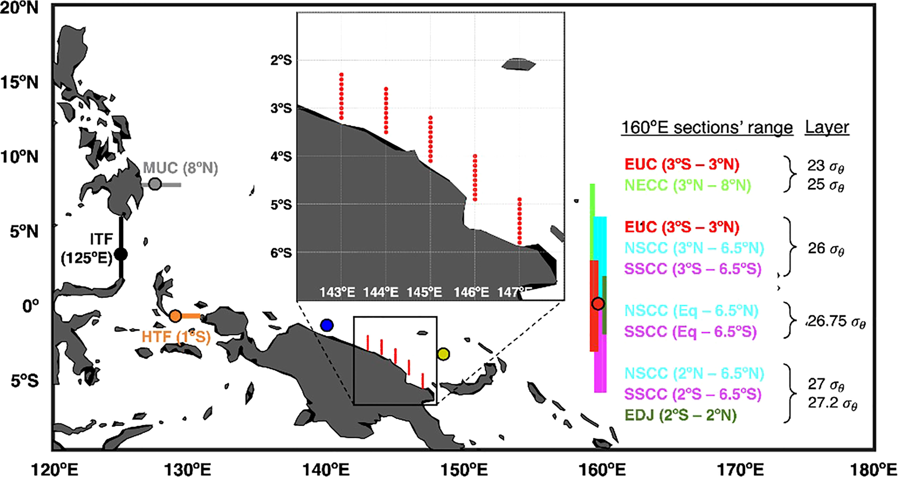
Figure 2 Experimental design of LPTM. The 50 red dots along the New Guinea coast are the locations where tracers were released. The color lines denote the location of the sections used to classify the tracers’ major destinations. Color circles denote the locations that are selected to estimate θ -S diagrams.
To classify the tracers’ destination, we defined a section at each designated current. We selected the section along 8°N (Mindanao coast – 130°N), 125°E (1.5° – 6°N), and 1°S (128° – 130.5°E) for MUC, ITF, and HTF, respectively. For the eastern route, we located the section along the longitude of 160°E. Placing the section too western may be difficult to distinguish the currents as some of them are typically found merging or are not even clearly formed yet far western (see Figure 1). On the other hand, placing the section farther east needs more time to arrive especially the tracers at the deeper layers (i.e., 27 and 27.2 σθ ), which may lead to reducing the number of tracers that are successfully classified. Please notice that the horizontal range of the same section could be disparate at the different layers and not all sections are defined in each isopycnal layer. It certainly depends on the currents’ vertical and horizontal ranges. The location and range of the sections that represent the tracer’s destination are provided in Figure 2.
3. Results
3.1. Validations of datasets
The reliability of the model results was first assessed by comparing them to observations and suggested that, overall, the models reproduce reasonably well the ADCP’s velocity profiles and their variability (see Figure 3). However, some notable discrepancies are clearly shown in OFES and HYCOM as compared to the observations, especially in simulating the weakening (strengthening) of the eastward-flowing EUC during the strong El Niño-Southern Oscillation (ENSO) event in 1997 (1998) (Figures 3I, O). Moreover, HYCOM seems to overestimate the northward-flowing MUC (Figure 3M). In comparison, the velocity profiles of GLORYS2V4 are in better agreement with the observed velocities in all regions.
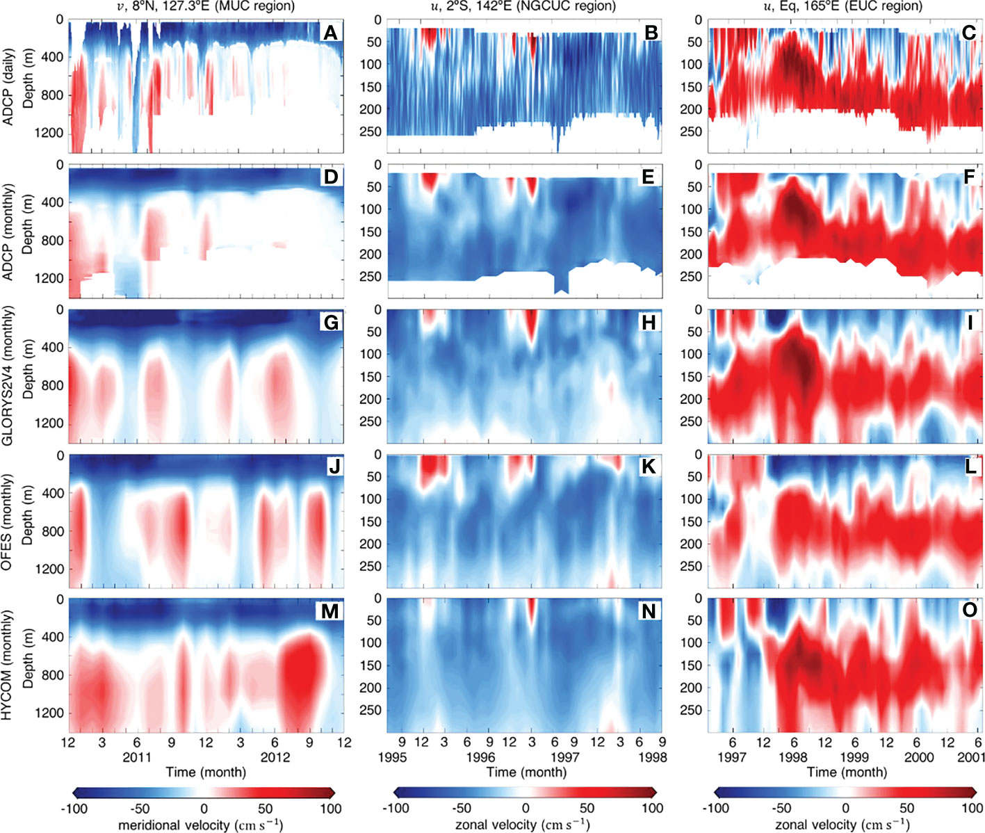
Figure 3 Time-depth sections of velocities (cm s-1) from [first-row panels (A-C)] daily ADCPs, [second-row panels (D-F)] monthly ADCPs, [third-row panels (G-I)] monthly GLORYS2V4, [fourth-row panels (J-L)] monthly OFES, and [fifth-row panels (M-O)] monthly HYCOM at approximately (left panels) 8°N, 127.3°E, (middle panels) 2°S, 142°E, and (right panels) Equator, 165°E. The left, middle, and right panels are meridional, zonal, and zonal velocities, respectively.
To further test the validity of the model results in representing the undercurrents, we compared their time series with that of the observations (Figure 4). We used monthly mean velocity data and selected the depths of 650, 200, and 150 m for the moored ADCP’s location deployed at the MUC, NGCUC, and EUC regions, respectively (see Figure 3). Based on the data used in these time series, we applied Taylor diagram analysis (Taylor, 2001) to examine how well each model matches the observation using three distinct statistics, i.e., centered RMSD, correlation coefficient, and STD. In the Taylor diagram, the closer the model is to the observation, which is represented by the RMSD, the better the model approximates the observation. This method determines the error (RMSD) that comes from the discrepancies in pattern similarity (correlation) or from the discrepancies in variance (STD). The results of the Taylor diagram clearly show that the GLORYS2V4 is closest to the observations at the MUC and EUC regions with the correlation coefficient of more than 0.6 and 0.8, respectively (see Figures 4B, F). In the NGCUC region, all models well approximate the observation with the correlation of more than 0.7. The GLORYS2V4 is slightly higher correlation than others. But, in terms of variance, HYCOM is closest to the observation. However, in this region, HYCOM seems to underestimate the eastward-flowing NGCC (see Figure 3N).
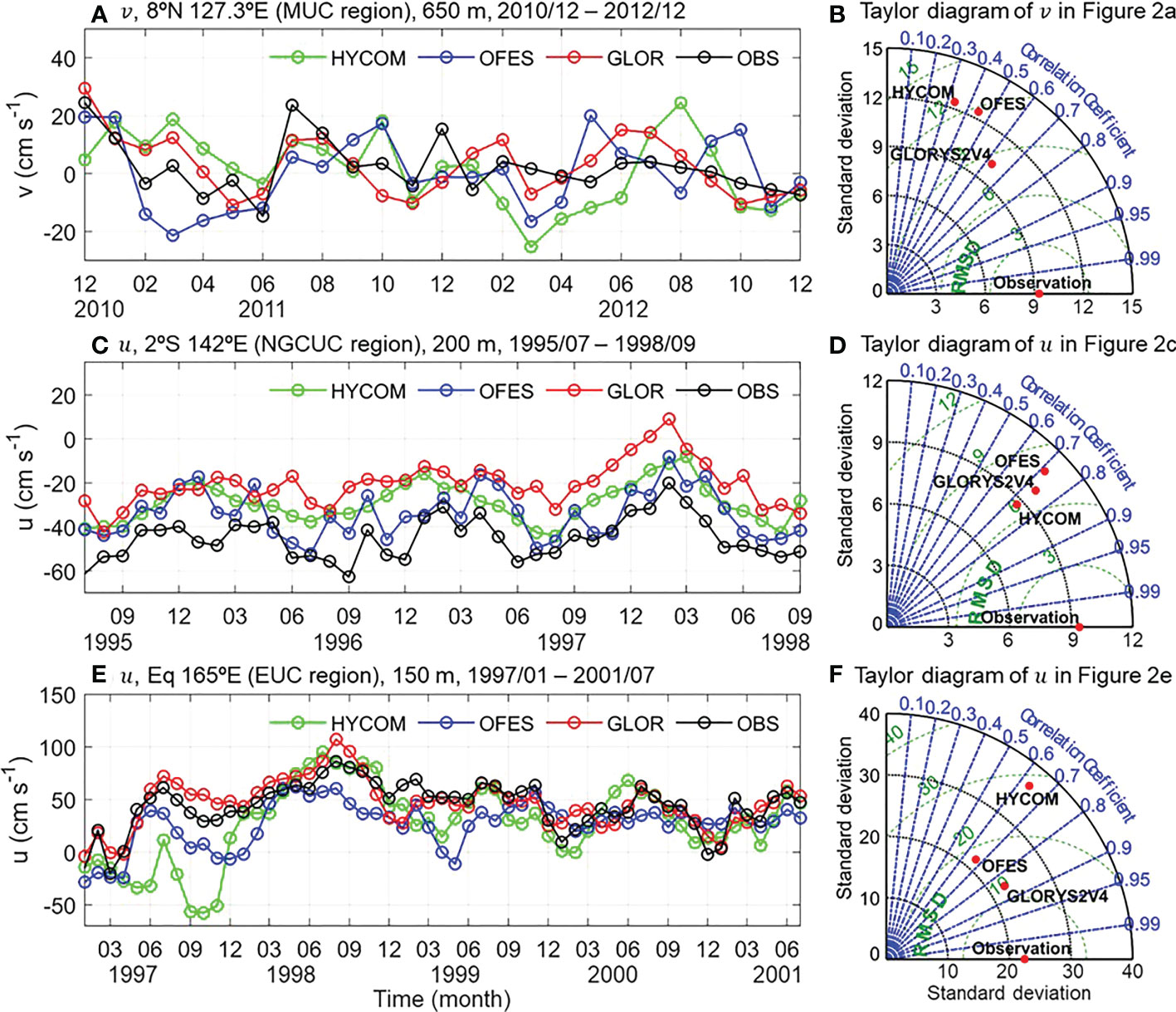
Figure 4 (A) Comparison of monthly meridional velocities (cm s-1) from mooring observation (black line) and the model outputs from GLORYS2V4 (red line), OFES (blue line), and HYCOM (green line) from December 2010 to December 2012 at approximately 8°N, 127.3°E and at the depth of approximately 650 m. (B) The Taylor diagram compares the velocities from mooring observation to the model outputs in Figure 4A. (C) and (D) are same as (A) and (B), respectively but monthly zonal velocities (cm s-1) from July 1995 to September 1998 at approximately 2°S, 142°E and at the depth of approximately 200 m. (E) and (F) are same as (A) and (B), respectively but monthly zonal velocities (cm s-1) from January 1997 to July 2001 at approximately Equator, 165°E and at the depth of approximately 150 m.
While the OFES and HYCOM datasets have been extensively used in a number of earlier studies to investigate ocean circulation in the WP (e.g., Chiang and Qu, 2013; Wang et al., 2016b; Nan et al., 2019; Wang et al., 2019; Zhang et al., 2020; Zhang et al., 2021), the GLORYS2V4 is less utilized in this region. Nevertheless, our results have shown that among the models GLORYS2V4 best approximates the observations in three different regions and thereby reasonably well reproduces the regional circulation around the WP. Therefore, we believe that the results of this study can provide a better view of the physical processes in the WTP. As such, in the present study, we only utilize the reanalysis data from GLORYS2V4, including the temperature, salinity, and horizontal velocities.
To evaluate the reliability of GLORYS2V4-based LPTM, we applied this analysis to track the trajectory of surface drifting buoys, obtained by the Global Drifter Program (see Elipot et al., 2022 and https://www.aoml.noaa.gov/phod/gdp/hourly_data.php for details). We selected 5 drifters deployed in the WTP to validate the LPTM analysis. The detailed information of the drifters used in this simulation, e.g., initial location, initial date, and tracking time, is provided in Supplementary Table 1. The surface zonal and meridional velocities from GLORYS2V4 were utilized in this LPTM simulation. Figure 5 shows the trajectories of both drifters (red line) and tracer-tracking results (blue line). In general, the result of LPTM can reasonably approximate the trajectory of the drifters, in agreement with the background surface currents (see Figure 1). Therefore, this result confirms the reliability of the LPTM in tracing water parcels in the WTP. The slight discrepancies may result from unresolved submesoscale dynamics, which is beyond the scope of our study, possibly due to spatial and temporal discretization of the model. Nevertheless, we believe that the LPTM is still reliable and the above limitation will not significantly change the final destination of the tracer.
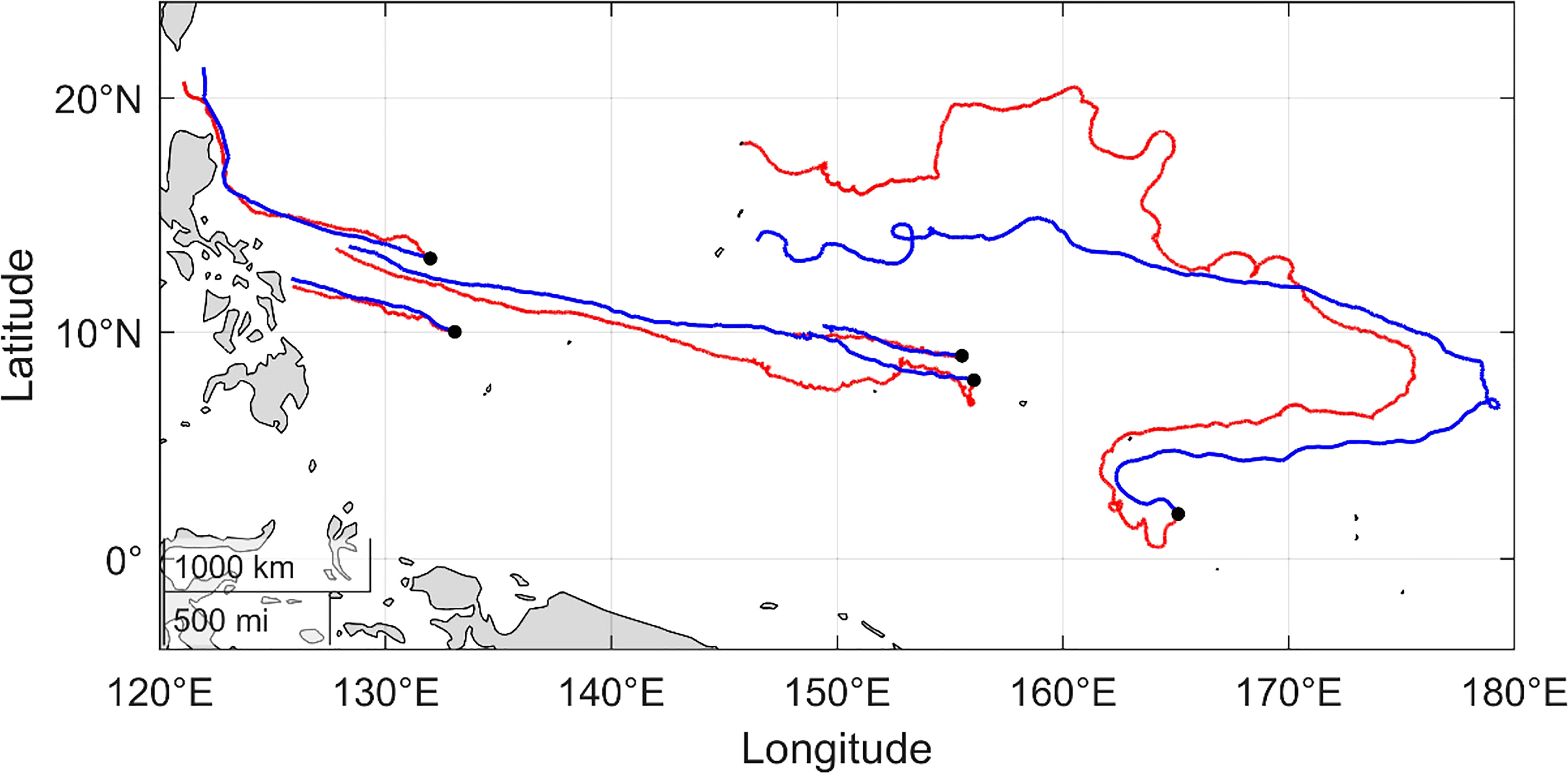
Figure 5 The trajectory of (red line) drifters and (blue line) LPTM results. The black dots denote the initial locations.
3.2. Mean structure
Before going into the results of the LPTM, it is beneficial to identify the mean structure of the currents that are possibly linked to the NGCUC. Figure 6 displays the vertical profiles of velocity overlaid with the contours of potential density at several sections. The results presented in this figure are based on model outputs from 1994 to 2015, where the first-, second-, and third-row panels are time average and composite during El Niño and La Niña phases, respectively. The sections were selected to show the typical structure of NGCUC and to preliminary identify its potential destinations. There are 180°E, 140°E, 125°E, 8°N, and 1°S sections to show the equatorial eastward currents (e.g., NECC, EUC, NSCC, SSCC, and EDJ), the NGCUC, the ITF, the MUC, and the HTF, respectively. In general, the vertical distribution of mean velocities from the model results shows consistency with previous studies (e.g., Qu et al., 2012; Wang et al., 2019; Delpech et al., 2020; Li et al., 2020; Zhang et al., 2020), displaying the typical formation of zonal or meridional velocities along each section.
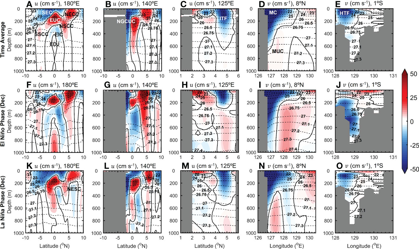
Figure 6 Latitude (longitude)-depth sections of zonal (meridional) velocities (cm s-1) from GLORYS2V4 along [first-column panels, (A, F, K)] 180°E, [second-column panels, (B, G, L)] 140°E, [third-column panels, (C, H, M)] 125°E, [fourth-column panels, (D, I, N)] 8°N, and [fifth-column panels, (E, J, O)] 1ºS. The first-, second-, and third-row panels are time average and composite during El Niño and La Niña phases, respectively, from January 1994 to December 2015. The black contours denote the zero velocity. The black dashed-contours denote the isopycnal layers (σθ), which are displayed for 22, 23, 24, 25, 26, 26.5, 26.75, 27, 27.1, 27.2, 27.3, and 27.4σθ.
The mean state of zonal velocity along 140°E shows that NGCUC ranges from nearly surface down to almost 800 m (or 27.2σθ ) and extends almost 200 km from the coast (Figure 6B). Please note that the wider range of westward flow near the surface is due to merging with SEC, instead of the wider NGCUC (Wang et al., 2019). The maximum of the mean westward velocity of approximately 68 ± 16 cm s-1 is found around the depth of 163 m (~25σθ ), which represents the NGCUC core.
In 180°E section (Figure 6A), a series of alternating zonal currents in the equatorial region is clearly shown, generally consistent with the results of previous studies (e.g., Delpech et al., 2020; Li et al., 2020). The result shows five eastward (i.e., NECC, EUC, NSCC, SSCC, and EDJ) and two westward (i.e., SEC and EIC) currents. The eastward currents shown in this figure are suspected to be the escape routes of the NGCUC waters into the central Pacific. Note that there might be some currents that do not appear in the mean state. For example, the westward core of EDJ (Delpech et al., 2020) and the westward-flowing NESC (Figure 6K, Li et al., 2020).
Multiple cores of ITF are shown along 125°E section (Figure 6C). The main core, which is centered at approximately 4.75°N, is a surface-intensified westward velocity (above 27σθ ) with the maximum mean velocity reaching 60 cm s-1. This core is mainly sourced from the MC that turns westward at the southern tip of Mindanao Island (Feng et al., 2018). Another core is much weaker (~3 cm s-1) and is centered at approximately 3.25°N and 27.2σθ . The source of this core is unknown yet but could be from the equatorial Pacific via NESC (Li et al., 2021) or from the South Pacific via NGCUC. The lower core of ITF along 125°E section will be further investigated in Section 3.3.
Figure 6E shows the vertical profile of southward-flowing HTF. In the mean state, this flow is quite strong with the maximum mean velocity reaching 68 cm s-1 near the surface. Along 1°S section, the HTF core is mainly centered at the western part of the channel (~128.5°E) along the east coast of Halmahera Island. The result in Figure 6J suggests that the velocity core of the HTF is revealed deepening during El Niño phase. A detailed analysis of this event will be described in section 3.5.
Section 8°N shows a core of northward-flowing MUC with the maximum mean velocity reaching 4.5 cm s-1 at the depth of around 560 m (Figure 6D). This core extends approximately 120 km offshore and is found below 400 m (or below ~26.75σθ ). Previous studies have confirmed that this current is a quasi-permanent current with strong intraseasonal variability, which is closely related to SE-1 and SE-2 activities (Azminuddin et al., 2022).
3.3. Destination of NGCUC
The destination of NGCUC is deduced from the trajectories of tracers released from the NGCUC region using LPTM. Figures 7A–F display the resulting trajectories that represent the pathways of tracers in all selected density layers. The color shading denotes the mean probability distribution of NGCUC water parcels at each grid cell (0.25°×0.25°). The probability was estimated as the ratio between the number of tracers passing through grid cells and the total number of tracers released. The grid cells with higher probability are the region where the tracers pass more frequently. This interpretation can identify the destination of NGCUC including predicting its water mass distribution. The results show that the dissemination of NGCUC tracers varies markedly with depth, but in general, most tracers are distributed to the east, which is consistent with previous studies (Wang et al., 2016b; Li et al., 2020; Zhang et al., 2020; Li et al., 2021).
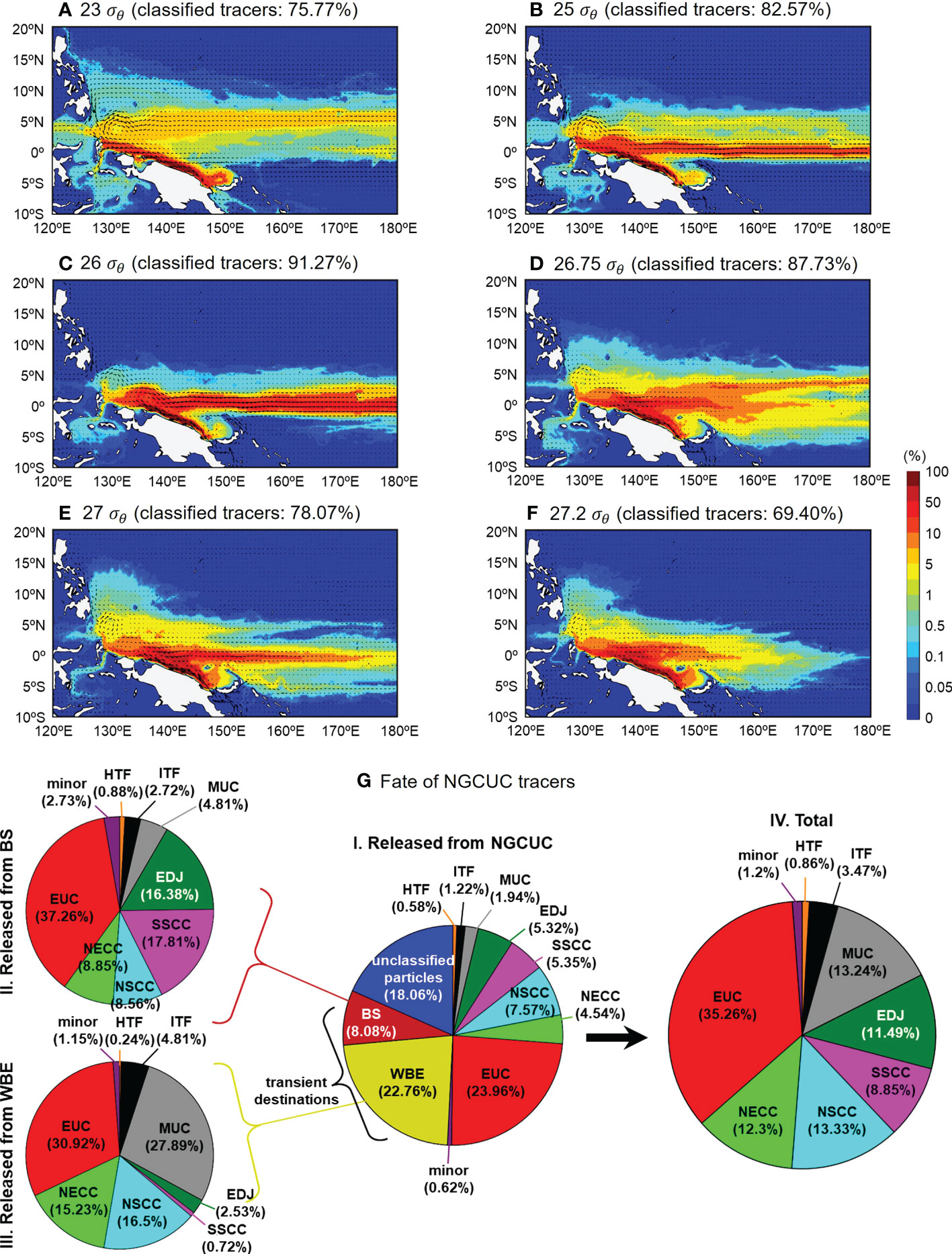
Figure 7 Mean probability distribution of tracers (%) released at the NGCUC region (see Figure 2 for the initial position of each tracer) at the isopycnal layers of (A) 23, (B) 25, (C) 26, (D) 26.75, (E) 27, and (F) 27.2 σθ . The tracers (50 tracers/layer) were released every day from 1994 to 2013 with the travel time of two years. The black arrows indicate current vectors. (G) Pie charts I, II, and III show the ratio of tracers’ destinations released directly from the NGCUC, BS, and WBE regions. Pie chart IV shows the ratio of tracers’ major and minor destinations from the total tracers released from the NGCUC region, including tracers that were temporarily trapped in the BS and WBE regions.
As described in Section 2.2, some predefined sections were selected to quantitatively classify the destination of each tracer (see Figure 2). The classification of the NGCUC tracers’ fate from all isopycnal layers is summarized in Figures 7G-I. Within two years’ travel time of tracer tracking, approximately 50.48%, 0.62%, and 30.84% of tracers are classified as major, minor, and transient destinations, respectively. Note that the total classified tracers into these destinations explain only 81.94% of the total tracers that were released daily from 1994 to 2013. The classified tracers are those that reach a predefined section, meaning the remaining unclassified portions (18.06%) do not pass through any predefined sections within the given travel time, possibly due to being slowed down by turbulence or the effect of a random-walk component in Eq. 1 that could suddenly change the direction of tracers’ motion before reaching any destinations.
The tracers classified as the transient destinations are those that are trapped in the Pacific Western Boundary Eddies (hereafter called the WBE, defined here as the HE and SE-2 regions) or the Bismarck Sea (BS). The present study considers both WBE and BS as transient destinations (or transit locations) rather than major destinations of NGCUC, in which the tracers need more travel time to escape from there and be redistributed into one of the major or minor destinations. The results show that approximately 22.76% (8.08%) of total tracers are trapped in the WBE (BS).
To confirm this assumption and to further identify the fate of tracers trapped in those transient destinations, we released tracers in both WBE and BS and applied the same scenario of LPTM (see Figures 7G-II-III). It implies that the portion of NGCUC tracers trapped in the WBE and the BS will be distributed according to these respective ratios. The maps of mean probability distribution of tracers released at these regions can be seen in Supplementary Figures 1 and 2. The result reveals an overall decrease (increase) in the tracers distributed to the eastern destinations for the WBE (BS)-originated tracers as compared to the NGCUC-originated tracers. Notably, the tracers distributed to the MUC account for more than one-fourth of all tracers released from the WBE (Figure 7G-III) – a much bigger slice of the destination pie than the tracers directly released from the NGCUC region (i.e., 1.94%) (Figures 7G-I). Consequently, the total ratio of NGCUC’s tracers distributed northward through the MUC increases up to 11.3% becoming 13.24% (Figure 7G-IV). A large portion of the WBE-originated tracers distributed to the MUC region is also clearly shown in Supplementary Figures 2D–F. This implies a critical role of eddy in trapping and transporting the NGCUC waters, and in connecting the NGCUC to the MUC, which is typically disconnected. A more detailed analysis of the WBE will be provided in Section 4.
By considering all NGCUC tracers directly originated from the NGCUC region, and the tracers temporarily trapped in the WBE and BS, the present study suggests the total destinations’ ratio of the NGCUC tracers as summarized in Figure 7G-IV and Table 1. The results confirm that a large amount of the NGCUC waters is distributed to the central Pacific through the EUC, NECC, NSCC, SSCC, and EDJ. It accounts for 81.65% of all tracers released. Most of the remaining portions are distributed westward into the MUC, ITF, and HTF. This result may reflect the distribution’s ratio of the total NGCUC transport.
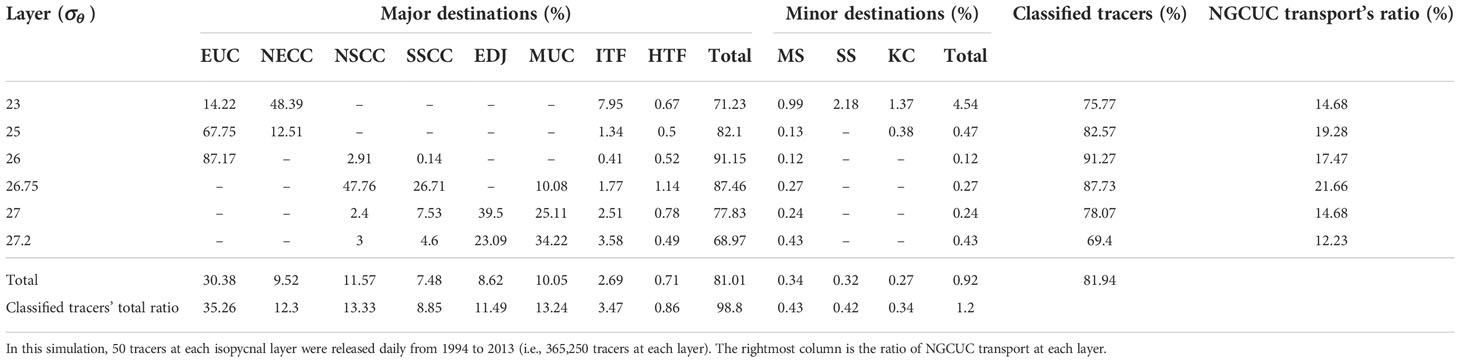
Table 1 Classification of tracers that were released at the NGCUC region within two years’ travel time, including the tracers that were temporarily trapped in the BS and WBE regions.
By means of LPTM, various destinations of NGCUC are observed, but only eight major destinations are further analyzed in the present study. There are NECC (12.3%), EUC (35.26%), NSCC (13.33%), SSCC (8.85%), EDJ (11.49%), MUC (13.24%), ITF (3.47%), and HTF (0.86%). These are suggested as the major destinations considering the relatively high percentage (>0.5%) and the persistency of tracers passing through their territory or tracks. In addition, it is also observed that a few portions of tracers move toward the Maluku Sea (MS) (0.43%) and the Solomon Sea (SS) (0.42%), and the KC (0.34%). The tracers distributed into these minor destinations (i.e., SS, MS, and KC) explain approximately 1.2% of the total tracers released. The finding of these minor destinations, especially the KC and the SS, is surprising and beyond what we expected at the beginning of this study. Note that the upper NGCUC waters can be advected back to the SS by the southeastward-flowing NGCC. We suggest that some tracers, especially above 25σθ , can be advected northwestward to the KC after joining the NECC to the east and then the NEC to the west possibly due to the strong NEC phase (see Figures 5, 7A, B). This implies a possible connection between the NGCUC and the KC. However, further investigations with observational evidence are required to confirm this finding.
The results of LPTM show that different isopycnal layers can have disparate distributions of NGCUC waters. Along the isopycnal layers of 23 and 25σθ , only about 75.77 and 82.57% of total tracers, respectively, are successfully classified as major destinations. Most of the remaining portions are instead being trapped in the HE and the BS. A similar situation may also apply for the deeper layer, but being trapped in the SE-3 and the BS. Please note that the percentage of classified tracers is not only affected by the eddy’s and the BS’s trapping effects but also by the velocity of the flow itself. At the deeper layer, the current’s velocity becomes slower and thus the tracers need more time to reach any destinations’ section. For this reason, the total classified tracers are getting lower at the deeper layer (see Table 1). The percentage of classified tracers may increase with longer travel time, but we believe that it will not significantly change the ratio of the major destinations.
In the probability map (Figures 7A–F), the spreading of tracers is clear. The results show that the majority of NGCUC’s water parcels turn eastward to the central Pacific through several eastward-flowing currents. However, their portions vary by isopycnal layers. Along the uppermost isopycnal surface (i.e., 23σθ ), more than 67% (19%) of total classified tracers are distributed toward the east into NECC (EUC) around 5°N (equator). In comparison, at the isopycnal layers of 25 and 26σθ , most of the tracers (82.5% and 95.6%, respectively) turn eastward along the equator representing the core of EUC. At the deeper layer (26.75σθ ), this prominent eastward core disparts into northern and southern branches representing NSCC (54.6%) and SSCC (30.5%), respectively. The probability map shows that a core of equatorial eastward flow re-emerges at the isopycnal layer of 27σθ representing EDJ (50.7%), while the NSCC and SSCC branches are vastly lessened. These three eastern destinations keep appearing at the deepest isopycnal layer (27.2σθ ) but with a shorter zonal extent and their cores seem to merge and are unclearly distinguished. Please notice that the vertical and latitudinal ranges of these eastern destinations are consistent with the result of the mean zonal velocity distribution shown in Figure 6A. Their cores are well represented by the tracer distribution, implying the reliability of the LPTM result.
The portions of tracers that are distributed to the western destinations (i.e., MUC, ITF, and HTF) also vary by isopycnal layers. Up to 13.24% of total classified tracers are distributed poleward along the Philippine coast joining MUC. This portion is evident at the isopycnal layers below 26.75σθ (see Figures 7D–F) and the tracers may reach up to 15°N. This probability distribution is consistent with the poleward extent of AAIW (up to 15°N along the Philippine coast), which originates from the South Pacific via NGCUC, reported by Qu and Lindstrom (2004).
Around 3.47% of tracers are distributed to the ITF entrance (Celebes Sea) mainly through the south of Talaud Islands. These tracers are evident in most layers but mainly distributed at the uppermost (23σθ ) and lowermost (27.2σθ ) isopycnal layers which explain about 11.2% and 5.2% of total classified tracers, respectively. This result is consistent with the distribution of mean westward flow along 125°E section that also shows the westward cores around both 23σθ and 27.2σθ isopycnal layers (see Figure 6C). The LPTM results confirm that the southern westward flows (2.5° – 4°N) are mainly sourced from the NGCUC, while that at the northern (4° – 5.5°N) is obviously mainly sourced from the MC.
Other portions of NGCUC tracers also enter the Indonesian Sea, but through the eastern passage via Jailolo Strait (i.e., HTF). The number of tracers crossing HTF’s section was only 0.86% from the total classified tracers. Although the percentage is relatively small, the results from LPTM confirm that the NGCUC tracers persistently pass through this route, especially at the upper layers. After entering the Jailolo Strait, the tracers flowed toward the eastern part of ITF route, including the Halmahera Sea, Seram Sea, Lifamatola Passage, and Banda Sea before finally arriving in the Indian Ocean through Ombai Strait or Timor Passage. South Pacific water advected into these Indonesian Seas through the HTF has been previously confirmed (e.g., Gordon et al., 2003), which is consistent with our results.
3.4. Spatiotemporal change of the destination
In Section 3.3, various destinations of the NGCUC have been identified. Nevertheless, the ratio of the destination may change over time. To identify the major signals that significantly control the spatiotemporal variation of the NGCUC destination, we applied the power spectral density function for the transport of the NGCUC and its major destinations. In most regions, the power spectrum results show peaks at seasonal and interannual periods (see Supplementary Figure 3). Further analyses using LPTM also confirm that the ratio of NGCUC destinations evidently changes with both timescales. Therefore, this study will focus mainly on seasonal and interannual variations.
3.4.1. Seasonal variation
Figure 8G shows the monthly climatology (1994 – 2015) of the volume transport anomaly of the NGCUC and its major destinations. The result confirms that there is seasonality in the NGCUC transport, in which the volume transport of NGCUC is greatest in August (boreal summer) and weakest in February (boreal winter), which is consistent with previous studies (e.g., Kuroda, 2000; Kawabe et al., 2008; Zhang et al., 2020). These studies have suggested that the seasonal variations of currents off the northern coast of New Guinea are closely related to the monsoon. In boreal summer (winter), the northwestward current is intensified (weakened) in response to the southeasterly (northwesterly) monsoonal winds. In this subsection, we mainly focus on how the destination of NGCUC waters changes seasonally.
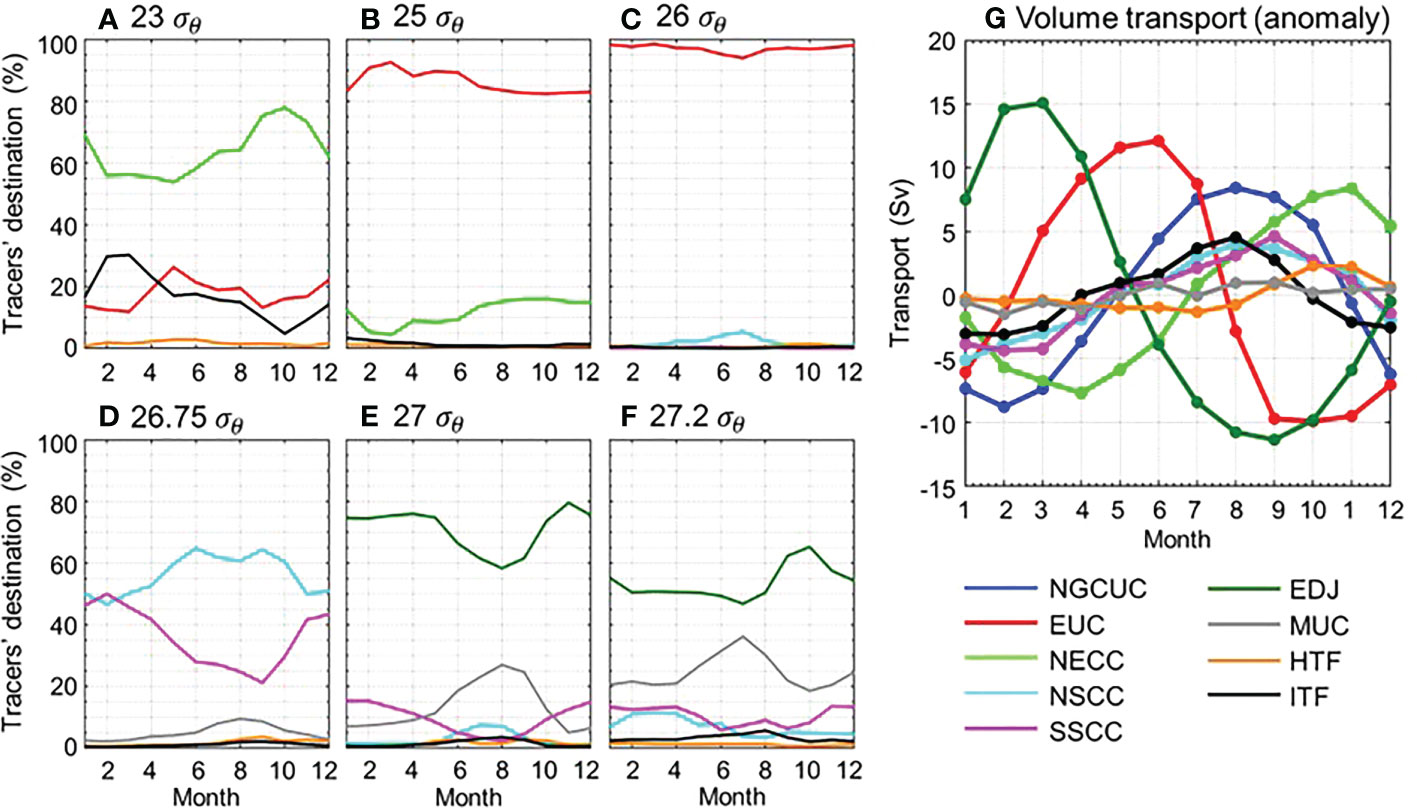
Figure 8 Monthly climatology (1994 – 2013) of the tracers’ ratio that arrived at the predefined sections of destination (%) at the density layers of (A) 23, (B) 25, (C) 26, (D) 26.75, (E) 27, (F) 27.2σθ . (G) Monthly climatology (1994 – 2015) of volume transport’s anomaly (Sverdrup) of NGCUC and its major destinations.
To evaluate the seasonal change of the NGCUC destination, we applied the LPTM to track the NGCUC tracers released in boreal summer (July – September) and boreal winter (December – February) from 1994 to 2013. The composite maps of the mean probability distribution of the NGCUC tracers during both seasons are shown in Figure 9. The results display the seasonal change of the pathways of tracers in all selected density layers. In some regions, the number of tracers’ distribution changes remarkably between summer and winter. Notably, along the 23 – 25σθ density layers (first- and second-row panels in Figure 9), the probability of tracers distributed to the NECC is higher in summer than in winter. At 26σθ density layer (third-row panel in Figure 9), where more than 87% of the NGCUC tracers are distributed to the EUC (Table 1), more tracers are distributed westward joining the HTF and the HE in summer than in winter. Below 26.75σθ (fourth-, fifth-, and sixth-row panels in Figure 9), the probability of tracers distributed poleward along the Philippine coast (i.e., MUC) is higher in summer than in winter.
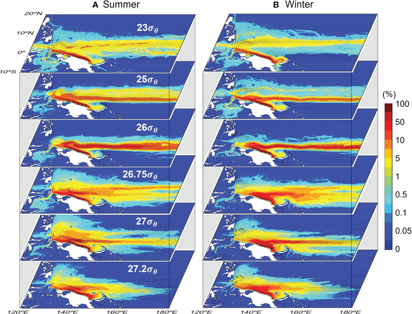
Figure 9 Composite map of mean probability distribution of NGCUC water parcels (%) at the isopycnal layers of 23, 25, 26, 26.75, 27, and 27.2 σθ . The probability at each layer was estimated from 50 tracers that were released around NGCUC region every day during (A) Summer and (B) Winter phases from 1994 to 2013 with the travel time of two years. The black arrows indicate current vectors.
To quantitatively analyze the seasonality of the NGCUC destination, we estimated the monthly climatology of the tracers’ ratio that arrived at each destination (Figures 8A–F). Note that the monthly ratio represents the percentage of tracers at a month when the tracers were released at the NGCUC region, not when they arrived at the destination. The results exhibit significant seasonal variations in some destinations which further confirm the results shown in Figure 9. The ratio of NGCUC tracers distributed to the NECC is highest in late summer (September – October) and is lowest in spring (May) and late winter (February – March) at 23 and 25σθ density layers, respectively (Figures 8A, B). The result also confirms that along 23σθ the ratio of NGCUC tracers distributed to the ITF is highest (lowest) in late winter (late summer), which is the opposite seasonality to the NECC at 23σθ and the ITF below 26.75σθ (Figures 8D–F). This indicates that the upper and lower cores of the ITF have different seasonality. In addition, the upper HTF shows a higher (lower) tracers’ ratio in early summer (winter). But that at the deeper layer doesn’t clearly show the seasonal variation.
Along 25σθ density layer, the seasonal change of tracers’ ratio distributed to the EUC and NECC reverse seasonally with a nearly opposite phase (Figure 8B). Although the tracers’ ratio of EUC upper 25σθ shows quite different seasonality, that at the 26σθ layer, which is the main location of the EUC core, shows a lower (higher) tracers’ ratio in summer (winter), which is the opposite seasonality to the NSCC at the same layer (Figure 8C). Along this isopycnal layer, the NSCC can also be considered as the lower part of the NECC (see Figure 6A). So, the tracers distributed northeastward after joining HE and becoming NECC at the upper layer can be represented by the tracers joining the NSCC at the lower layer and their seasonality is generally consistent with each other. Below 26σθ , the seasonal change of the NGCUC destinations can be clearly seen. The tracers’ ratio of NSCC and MUC (SSCC and EDJ) is higher (lower) in summer and is the opposite in winter.
In summary, in summer more NGCUC tracers are distributed westward and northeastward increasing the ratio of NECC, NSCC, MUC, upper HTF, and lower ITF. While in winter more NGCUC tracers are distributed eastward increasing the ratio of EUC, SSCC, and EDJ. These results imply that the seasonality of the NGCUC strength may influence the seasonality of its water distribution. During summer, the strengthened NGCUC brings the more water further northwestward than the typical state. While during winter, when the NGCUC flow is weak, most waters turn clockwise to spread eastward decisively along the equator.
3.4.2. Interannual variation
Located in the equatorial WP, the interannual variability of the NGCUC destination is most likely related to the ENSO cycle. Zhang et al. (2020) confirmed that the NGCUC exhibits interannual variations associated with ENSO, in which its velocity core shoaling (deepening) during El Niño (La Niña), consistent with our results (see Figures 6G, L). In terms of volume transport, although weak, our result suggests that the NGCUC is negatively correlated with the ENSO cycle with the correlation coefficient of -0.36, estimated from 22 years monthly mean GLORYS2V4 outputs and Ocean Niño Index (ONI) 3.4.
To investigate how the spreading of the NGCUC waters varies interannually, we also applied the LPTM to track the NGCUC tracers released in El Niño and La Niña phases from 1994 to 2013. There were four El Niño (i.e., 1994/1995, 1997/1998, 2002/2003, and 2009/2010) and six La Niña (1995/1996, 1998/1999, 1999/2000, 2007/2008, 2010/2011, and 2011/2012) events during the whole time series from 1994 to 2013. The composite maps of mean probability distribution of the NGCUC tracers during El Niño and La Niña are shown in Figure 10. The results demonstrate the different pathways of tracers between El Niño and La Niña events in all selected isopycnal layers.

Figure 10 Same as Figure 8 except the tracers were released during (A) El Niño and (B) La Niña.
Note that in this LPTM simulation, the movement of tracers is fully controlled by ocean currents. This implies that the distribution of NGCUC tracers can reflect the strengthening or weakening of its destinated currents. For example, during El Niño, the NECC is strengthened (Figure 6F), at the same time the portion of NGCUC tracers into NECC is greater than that in La Niña phase (first-row panels in Figure 10). Along 25 – 26σθ density layers (second- and third-row panels in Figure 10), the probability of tracers distributed to the EUC is much higher in the La Niña than that in El Niño, which coincides well with the strong eastward-flowing EUC during La Niña (Figure 6K). These results suggest that, interannually, the distribution of the NGCUC water is controlled by the strength of its destination currents associated with the ENSO cycle, in which more (less) NGCUC tracers are distributed to the strengthened (weakened) currents.
To quantitatively analyze the interannual change of the tracers’ distribution, we estimated the daily time series of the ratio (%) of the tracers that arrived at the predefined sections from 1994 to 2013 and compared the results to the ONI 3.4 as shown in Figure 11. Note that the ratio represents the percentage of tracers on a day when the tracers were released at the NGCUC region, not when they arrived at the destination. The right panels denote the box plot of the time lag (days), which is the travel time from the NGCUC region to arrive at the predefined sections.
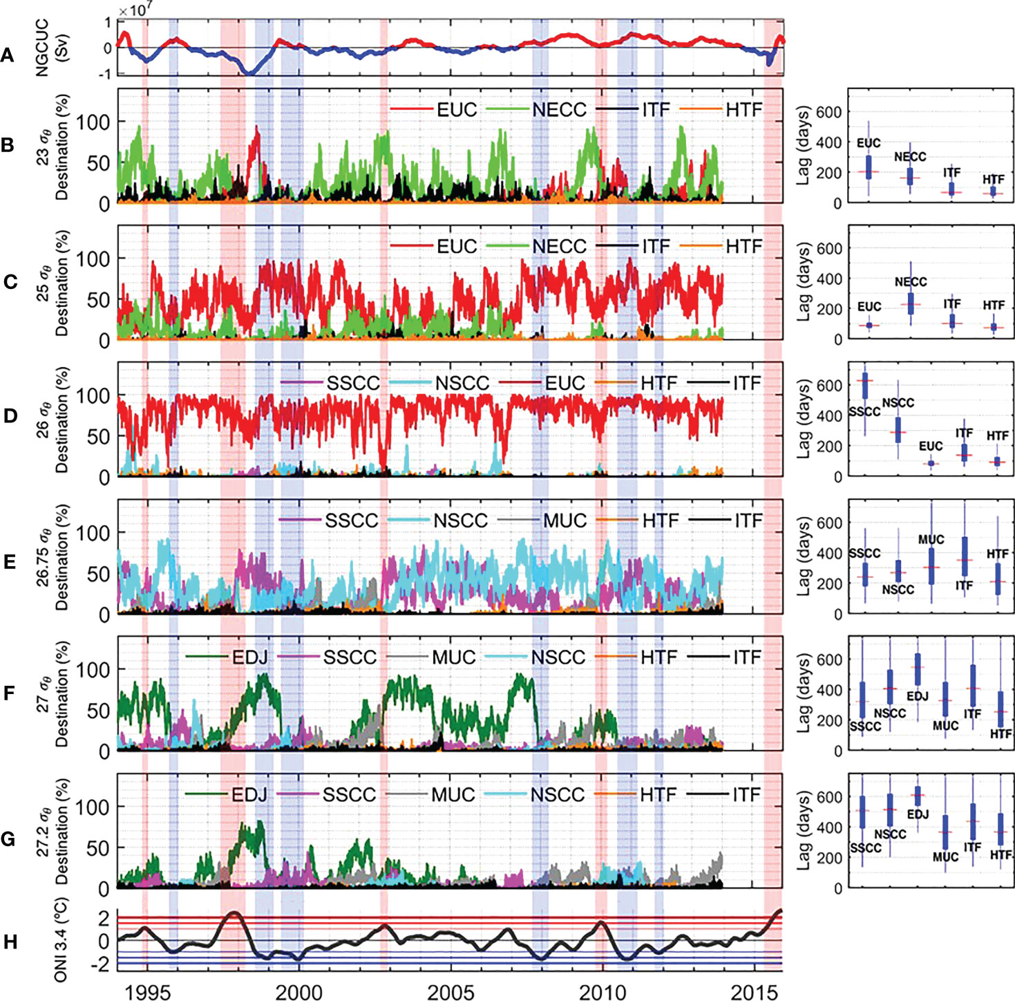
Figure 11 (A) The NGCUC transport’s anomaly (Sverdrup) from 1994 to 2015. Percentage of the tracers released from the NGCUC region that arrived at the predefined sections of destination from 1994 to 2013 at the isopycnal layers of (B) 23, (C) 25, (D) 26, (E) 26.75, (F) 27, and (G) 27.2σθ . The right panels are box plot of the time lag (days), which is the travel time from the NGCUC region to arrive at the predefined sections. (H) Ocean Niño Index 3.4 (°C) from 1994 to 2015.
In general, the time series of tracers’ ratio in most destinations exhibits no significant correlation with ENSO. But in some cases, the strong ENSO event may significantly change the distribution of the tracers. The 1997 – 1999 El Niño/La Niña phase is among the most remarkable ENSO event. A notable change in the tracers’ distribution can be observed during this event. During the 1998/1999 La Niña event, most NGCUC tracers at the upper layer (23σθ ), which typically feed the NECC (see Figure 7A), shift equatorward becoming EUC, which is indicated by a significant increase in the tracers’ ratio of EUC in 1998 (red line in Figure 11B), possibly due to the weakening of the NECC and strengthening of the EUC. It implies the vertical movement of the EUC core from 26σθ to 23σθ , closing the surface. This remarkable event was evidently observed by a moored ADCP, which was also well reproduced by the GLORYS2V4 model, as shown in Figures 3C, F, I. A similar situation may also occur during the 2009 – 2011 El Niño/La Niña event that shows a shoaling core of the EUC in 2010, but not as strong as that in 1998.
The results shown in Figures 11B, C further confirm that the El Niño events do not significantly increase the number of NGCUC tracers going into the NECC, considering the increasing number of these tracers also occurred in other periods, e.g., in summer 2006 and 2012. But these results highlight the particular impact of La Niña in decreasing the tracers going into the NECC as clearly shown in all six La Niña events. On the other hand, Figures 11B–D also show that La Niña does not play a role in increasing the number of NGCUC tracers going into the EUC, but the ratio of the EUC decreases in El Niño events, especially clearly seen at the 26σθ isopycnal layer. In summary, our results suggest that the ENSO cycle can meridionally shift the NGCUC waters that are distributed eastward, in which most of its eastward-distributed waters shift northward (equatorward) in El Niño (La Niña) phase joining the strengthened NECC (EUC).
3.5. Water mass transformation
Although LPTM has been able to estimate the spatiotemporal change of NGCUC’s destinations, the real distribution of NGCUC water mass at each destination has remained to be clarified. We then further analyze the water mass characteristics at each region by using θ -S diagram. Figures 12A, B display θ -S diagrams at the NGCUC region and its major destinations, which are estimated from model outputs and averaged from 1994 to 2015. To estimate the θ -S diagram, a point, where tracers pass more frequently, is selected as a proxy for each destination (i.e., 1.5°S, 140°E [NGCUC]; 8°N, 127.5°E [MC/MUC]; 1°S, 128.75°E [HTF]; 3.25°N, 125°E [ITF]; 3.5°S, 148.5°E [BS]; equator, 160°E [EUC/EDJ], see Figure 2).
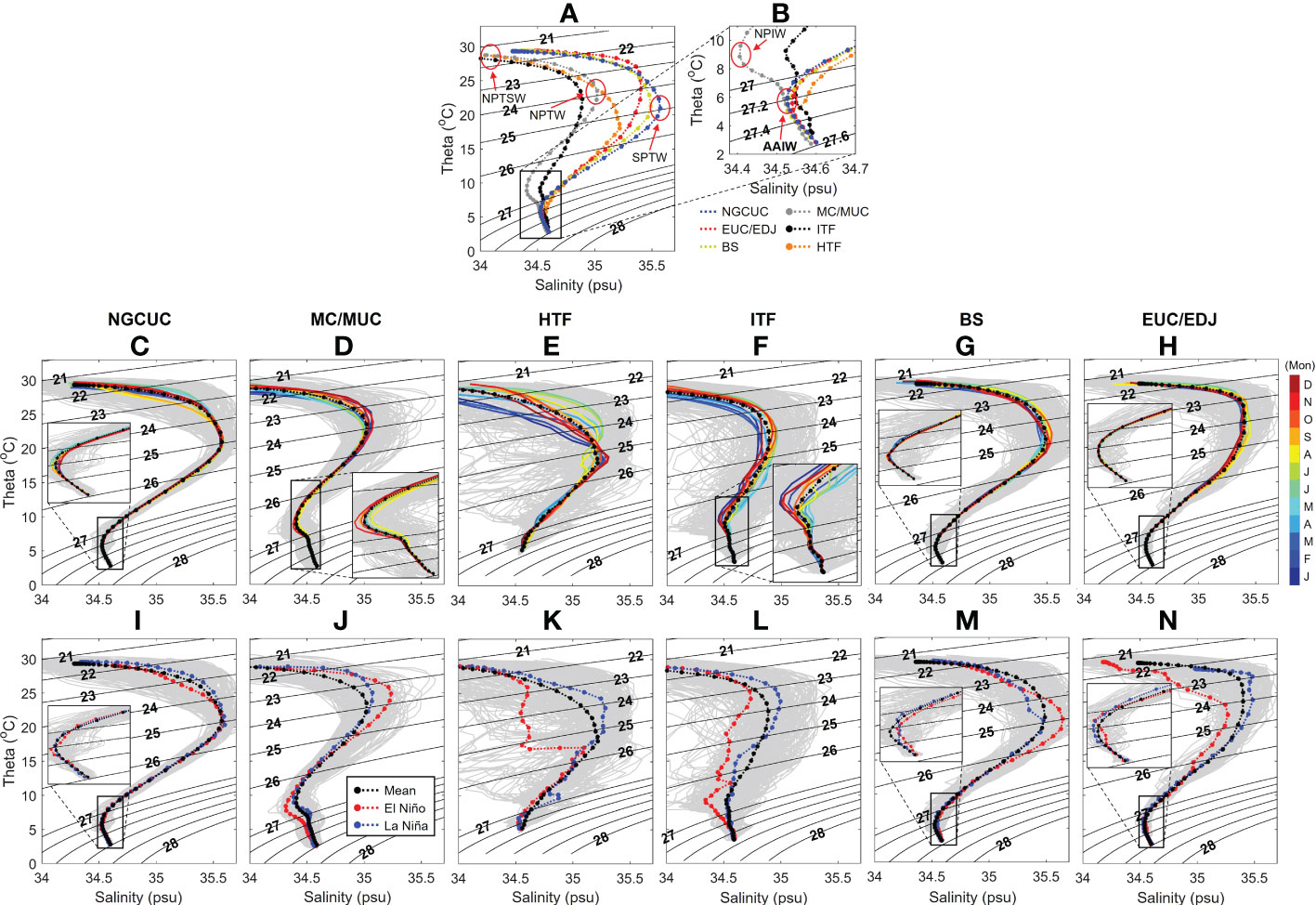
Figure 12 (A) θ -S diagrams at six locations (i.e., 1.5°S, 140°E [blue, NGCUC]; 8°N, 127.5°E [grey, MC/MUC]; 1°S, 128.75°E [orange, HTF]; 3.25°N, 125°E [black, ITF]; 3.5°S, 148.5°E [yellow, BS]; equator, 160°E [red, EUC/EDJ], see Figure 2) estimated from model outputs and averaged from 1994 to 2015. (B) Same as (A) but for the θ -S ranges of black rectangular that shown in (A). Except (A) and (B), the first- to sixth-column panels represent the θ -S diagrams at NGCUC (C, I), MC/MUC (D, J), HTF (E, K), ITF (F, L), BS (G, M), and EUC/EDJ (H, N) regions, respectively. The second- (third-) row panels are θ -S diagrams with monthly climatology (ENSO) phases. In the second- and third-row panels, the daily (mean) θ -S diagrams along whole period are shown by grey (black) lines.
Based on θ -S diagram analysis, the upper NGCUC water is characterized by a salinity maximum core (>35.1 psu) centered at 25σθ representing the SPTW that originates from the subtropical South Pacific (Fine et al., 1994; Qu et al., 1999). At the intermediate layer, NGCUC carries AAIW, which is characterized as salinity minimum water (34.55 psu) at 27.2σθ , originating from the Antarctic convergence zone (Qu and Lindstrom, 2004). The signatures of SPTW and AAIW, which are carried by NGCUC, can be found in most of the selected θ -S diagram points but with various transformations. Along 25σθ , the SPTW carried by the NGCUC is transformed into fresher water at BS and EUC regions. While at the other regions (i.e., HTF, ITF, and MC), the upper-layer water is mainly characterized by the fresher water NPTW, instead of the SPTW. It implies that upper-layer waters at the Pacific equatorial western boundary are mainly sourced from the MC that carries the NPTW.
At the MC/MUC region (8°N, 127.5°E), the θ -S diagram is characterized by the North Pacific waters, which is obvious, including the North Pacific Tropical Surface Water (NPTSW, a surface salinity minimum), the North Pacific Tropical Water (NPTW, a subsurface salinity maximum in the thermocline), and the North Pacific Intermediate Water (NPIW, a salinity minimum in the subthermocline) (Grey line in Figure 12B). However, below 27σθ the South Pacific water, i.e., AAIW, is confirmed, which is consistent with previous studies (e.g., Bingham and Lukas, 1994; Fine et al., 1994; Wang et al., 2016a). The results in Figures 6D and 12B suggest that in this region the fresher water NPIW is carried by the southward-flowing MC and the saltier water AAIW is transported by the northward-flowing MUC below 26.75σθ . The possible mechanism of how the South Pacific waters are transported to the Philippine coast has been suggested in our previous study (Azminuddin et al., 2022), which is carried by the NGCUC and the SE-2. This result is also well represented by the LPTM results in Section 3.3, implying the reliability of the particle tracking method.
Figures 12C–H show the θ -S diagrams with climatologically monthly mean (color θ -S diagrams) in all locations. The seasonal change of the water mass properties is clearly found in some regions, especially in the HTF region (Figure 12E). The results show that at the upper 24.5σθ , the HTF water transforms from relatively warm and salty water in summer to colder and fresher water in winter. This implies that during summer when the NGCUC is strengthened, the upper layer of HTF is transformed into saltier water possibly carrying the SPTW from NGCUC. While in winter, the upper layer of HTF is mainly sourced from the NPTW, which is characterized by relatively cold and fresh water. Note that this seasonal change is altered around the isopycnal layers of 25 – 25.7σθ . The results of LPTM further confirm that at the isopycnal layer of 23σθ the tracers are distributed more to the HTF in summer than in winter, but the case is reversed at the isopycnal layer of 25σθ (see first- and second-row panels in Figure 9). This result suggests that seasonal changes in the NGCUC strength can substantially magnify the seasonal water mass transformation of the HTF.
The interannual change of the θ -S diagrams at each region is also estimated as shown in Figures 12I–N. The black, red, and blue lines denote the time average and composite during El Niño, and La Niña, respectively, from 1994 to 2015. The AAIW at the MUC region is clearly defined in the La Niña phase. But the clarity is slightly lessened, which is fresher during El Niño years possibly mixing with the fresher water of NPIW. Figure 6I confirms that during El Niño the MC is strengthened and deepened, shifting the MUC further offshore. This event may transport more North Pacific waters to the MUC region and transform the intermediate water mass into becoming NPIW.
Figure 12K displays a noticeable water mass transformation of the HTF associated with the ENSO cycle, in which the upper HTF water is transformed into colder and fresher (warmer and saltier) water in the El Niño (La Niña) phase. This result implies that in addition to the NPTW and SPTW, the upper HTF can be sourced from another region. During La Niña (stronger NGCUC), more SPTW waters enter the HTF resulting in warmer and saltier water. However, during El Niño the source of fresh and cold waters that lead to a unique water mass remains uncertain. It can be either from NPTW or Indonesian Seas (e.g., Banda Sea). Koch-Larrouy et al. (2006) confirmed that the Banda Sea is characterized by a relatively constant salinity (around 34.58 psu) below 20°C. This is consistent with the upper HTF water during El Niño phase (red line in Figure 12K). Moreover, the velocity core of the HTF is revealed deepening during El Niño phase (see Figure 6J), and its velocity upper 25.5σθ reverses becoming a northward current, flowing from the Indonesian Sea to the Pacific Ocean. So, we suggest that during El Niño the upper HTF water mainly comes from the Banda Sea.
4. Discussion
The uncertainty of water masses’ movement in the ocean is tightly linked to turbulence or eddy. Previous studies have confirmed various effects of mesoscale eddies on ocean circulation by, for example, influencing their strength (Azminuddin et al., 2022), transport (Lien et al., 2014), and generation (Qiu et al., 2013; Qiu et al., 2015). The eddies also act as an “underwater mixer” of intermediate waters (Nan et al., 2019). Unlike current that transports water masses continuously, eddy can trap fluid parcels within its core and transport them discretely (Zhang et al., 2014), thereby complicating the assessment of the spreading of NGCUC water mass.
To evaluate the contributions of eddies to the NGCUC’s pathways, we released tracers at the core of the Pacific WBE at each density layer as shown in Supplementary Figure 2. In addition, we also estimated the travel time of the tracers (see Figure 13). These experimental approaches enable us to explore how long the NGCUC tracers are trapped in the Pacific WBE and how the trapped tracers are dispersed in the WTP. To identify the strength and core location of an eddy, we applied eddy kinetic energy (EKE) and Okubo-Weiss parameter (OWP) methods following Azminuddin et al. (2021). The OWP identifies eddy by quantifying the relative contribution of deformation and vorticity in the fluid flow. In this study, we selected the threshold value of 5×10-12 s-2 to define the eddy boundary.
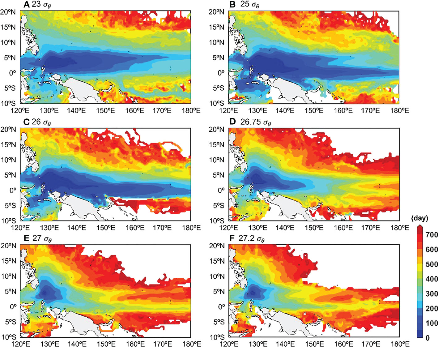
Figure 13 Mean travel time distribution of tracers (day) released at the WBE region at the isopycnal layers of (A) 23, (B) 25, (C) 26, (D) 26.75, (E) 27, and (F) 27.2 σθ . The tracers (50 tracers/layer) were released every day from 1994 to 2013 with the travel time of two years.
The results of the mean probability distribution map show that the tracers released from the WBE are distributed to similar destinations to those released from the NGCUC (except the BS and SS), but with different ratios (see Figure 7 and Supplementary Figure 2). It is obvious that no (or very rare) tracer is found in the New Guinea coast, BS, and SS regions, in which the tracers are blocked by the northwestward-flowing NGCUC. The ratio of the tracers’ distribution has been detailed in Section 3.3. The result reveals an overall increase in the tracers distributed to the western destinations for the Pacific WBE-originated tracers as compared to the NGCUC-originated tracers. But still, most tracers released at the Pacific WBE are distributed eastward (> 66%). This implies that the presence of eddy enables the westward-distributed waters to return eastward, indicating the role of eddies in redistributing the NGCUC water.
The contribution of eddies to the NGCUC’s pathways can be explained in part by estimating the transit time of tracers in the WBE that represents the trapping effect of the eddy. In this study, we define the transit time as the period (in days) of tracers to escape from the WBE. The results confirm that the transit time is getting longer at the deeper isopycnal layer (Figure 13), which is obvious as the water flow is getting slower in the deeper layer. The mean transit time of tracers in the WBE is approximately 34, 45, 49, 78, 102, and 107 days at the 23, 25, 26, 26.75, 27, and 27.2σθ isopycnal layers, respectively. In relation to the eddy strength, the results confirm that the tracers typically stay longer (shorter) in the WBE with lower (higher) EKE. So, the strengthened (weakened) WBE, which has faster (slower) water flow, traps the tracers shorter (longer).
Although the turbulence-driven dispersion of water parcels is not fully resolved in model outputs due to spatial and temporal discretization (Rühs et al., 2018), a random walk component () with the Smagorinsky diffusivity scheme was applied in the LPTM to approximate unresolved processes, e.g., sub-grid scale turbulent motion (North et al., 2006). Therefore, the results of LPTM can reasonably capture the path of tracers that were trapped and redistributed by the Pacific WBE. We believe that unresolved processes due to eddy (turbulent) diffusion do not significantly change the total ratio of the NGCUC destination, considering the dominance of eastern destination currents (i.e., EUC, NECC, NSCC, SSCC, and EDJ), which are robust. Nevertheless, future studies need to take this into account.
In addition, WBE also plays an important role in linking the currents. The HE has been widely known to link the NGCUC to the NECC (Arruda and Nof, 2003). The results further confirm that below the surface this prominent eddy partially connects the NGCUC to the EUC and the NSCC, in which some tracers temporarily trapped in the HE were also distributed to these eastward flows. The present study suggests another fundamental linkage below the surface. The results confirm that the NGCUC can also be connected to the MUC by the SE-2. Unlike the HE, which continuously links the currents owing to its quasi-permanent nature and larger scale, this undercurrent linkage is intermittently connected, which highly depends on the NGCUC strength and behavior of the SE-2. Further analysis of these eddy-related current linkages is beyond the scope of the present study and is important as a subject for future studies.
5. Summary
The NGCUC spreads South Pacific water into the North Pacific, influencing the circulation and water mass characteristics. Therefore, it is important to investigate the geographical distribution of the NGCUC waters and its spatiotemporal changes to better understand the evolving circulation and water mass characteristics in the WTP.
The destination of NGCUC was deduced from the trajectories of tracers released from the NGCUC region daily from 1994 to 2013 with two years of travel time using forward LPTM. The lagrangian diagnostics allow us to document the lifecycle of NGCUC tracers before arriving at any destination including splitting, merging, and interacting with eddies. In general, the destinations of South Pacific waters carried by NGCUC into the NWP can be divided into two escape routes: the eastern and western routes. The western route is divided into the northwestern route and the Indonesian Seas route. Within these routes, we reveal eight major destinations of NGCUC: EUC (35.26%), NECC (12.3%), NSCC (13.33%), SSCC (8.85%), EDJ (11.49%), MUC (13.24%), ITF (3.47%), and HTF (0.86%). In addition, the particle tracking results suggest that a few portions of NGCUC waters are also distributed to three minor destinations, i.e., MS (0.43%), SS (0.42%), and KC (0.34%).
The ratio of NGCUC destinations exhibits pronounced seasonal variations closely associated with the seasonal change of the NGCUC strength. The NGCUC strengthens (weakens) during summer (winter) and more NGCUC waters are distributed westward and northeastward (eastward) into the MUC, lower ITF, upper HTF, NECC, and NSCC (EUC, SSCC, and EDJ). In addition, the results reveal that on interannual timescales the distribution of the NGCUC water is controlled by the ENSO cycle that modulates the strength of the currents linked with the downstream NGCUC. Most of its eastward-distributed waters shift northward (equatorward) in El Niño (La Niña) phase joining the strengthened NECC (EUC). These spatiotemporal changes of the NGCUC destination contribute to the water mass characteristics and their seasonal and interannual transformations. Detailed dynamic processes associated with the spatiotemporal changes of the NGCUC destination will be investigated in further studies.
Approximately 22.76% (8.08%) of tracers were temporarily trapped in the equatorial Pacific WBE (BS) before being redistributed. In the present study, the effects of eddies on the pathways of NGCUC’s waters are evaluated. The results suggest that eddies could regionally affect water mass properties by trapping and redistributing the water mass. The presence of eddy enables the westward-distributed NGCUC waters to return eastward. Finally, the results suggest the fundamental role of the Pacific WBE in linking the currents in the equatorial WP, including the SE-2 that links the NGCUC to the MUC.
Data availability statement
The datasets presented in this study can be found in online repositories. The names of the repository/repositories and accession number(s) can be found below: The mooring data used in this study were provided by the Northwestern Pacific Ocean Circulation and Climate Experiment (NPOCE) (http://npoce.org.cn/dateAcc.aspx) and the Tropical Ocean Climate Study (TOCS) (https://www.jamstec.go.jp/e/database/ocean.html) programs. The GLORYS2V4 data are freely available from Mercator Ocean (https://doi.org/10.48670/moi-00024). The HYCOM data are freely available from the HYCOM consortium (http://www.hycom.org/dataserver/gofs-3pt1/reanalysis). The OFES data are freely available from APDRC Live Access Server (http://apdrc.soest.hawaii.edu/las_ofes). The drifter data are freely available from NOAA-AOML (https://www.aoml.noaa.gov/phod/gdp/hourly_data.php).
Author contributions
FA proposed the main ideas, collected the data, performed the data analysis, and wrote the original manuscript. CJ critically reviewed the data analysis results. All authors participated in the discussion, contributed to the improvement of the manuscript, and approved the submitted version.
Funding
This study was supported by the projects titled Korea-China Joint Ocean Research Center (20220407)” and “KIOS (Korea Indian Ocean Study): Korea-US Joint Observation Study of the Indian Ocean (20220548, PM63180)” funded by the Korean Ministry of Oceans and Fisheries, Korea, and the project titled "Projection and evaluation of ocean climate and extreme events based on AR6 scenarios (KMI2021-01511)" funded by the Korea Meteorological Administration.
Conflict of interest
The authors declare that the research was conducted in the absence of any commercial or financial relationships that could be construed as a potential conflict of interest.
Publisher’s note
All claims expressed in this article are solely those of the authors and do not necessarily represent those of their affiliated organizations, or those of the publisher, the editors and the reviewers. Any product that may be evaluated in this article, or claim that may be made by its manufacturer, is not guaranteed or endorsed by the publisher.
Supplementary material
The Supplementary Material for this article can be found online at: https://www.frontiersin.org/articles/10.3389/fmars.2022.1080314/full#supplementary-material
References
Arruda W. Z., Nof D. (2003). The Mindanao and halmahera eddies – twin eddies induced by nonlinearities. J. Phys. Oceanogr. 43, 2815–2830. doi: 10.1175/1520-0485(2003)033<2815:TMAHEE>2.0.CO;2
Azminuddin F., Jeon D., Kim Y. H., Jang C. J., Park J.-H. (2021). A newly observed deep countercurrent in the subtropical northwest pacific. J. Geophys. Res. Oceans 126, e2021JC017272. doi: 10.1029/2021JC017272
Azminuddin F., Lee J. H., Jeon D., Shin C.-W., Villanoy C., Lee S., et al. (2022). Effect of the intensified sub-thermocline eddy on strengthening the Mindanao undercurrent in 2019. J. Geophys. Res. Oceans 127, e2021JC017883. doi: 10.1029/2021JC017883
Bingham F. M., Lukas R. (1994). The southward intrusion of north pacific intermediate water along the Mindanao coast. J. Phys. Oceanogr 24, 141–154. doi: 10.1175/1520-0485(1994)024%3C0141:TSIONP%3E2.0.CO;2
Chassignet E. P., Hurlburt H. E., Metzger E. J., Smedstad O. M., Cummings J. A., Halliwell G. R., et al. (2009). US GODAE: Global ocean prediction with the HYbrid coordinate ocean model (HYCOM). Oceanography 22 (2), 64–75. doi: 10.5670/oceanog.2009.39
Chiang T.-L., Qu T. (2013). Subthermocline eddies in the Western equatorial pacific as shown by an eddy-resolving OGCM. J. Phys. Oceanogr. 43, 1241–1253. doi: 10.1175/JPO-D-12-0187.1
Chiang T.-L., Wu C.-R., Qu T., Hsin Y.-C. (2015). Activities of 50–80 day subthermocline eddies near the Philippine coast. J. Geophys. Res. Oceans 120, 3606–3623. doi: 10.1002/2013JC009626
Choi J.-G., Jo Y.-H., Moon I.-J., Park J., Kim D.-W., Lippmann T. C. (2018). Physical forces determine the annual bloom intensity of the giant jellyfish Nemopilema nomurai off the coast of Korea. Reg. Stud. Mar. Sci. 24, 55–65. doi: 10.1016/j.rsma.2018.07.003
Delpech A., Cravatte S., Marin F., Morel Y., Gronchi E., Kestenare E. (2020). J. Phys. Oceanogr 50, 281–304. doi: 10.1175/JPO-D-19-0132.1
Dormand J. R., Prince P. J. (1980). A family of embedded runge-kutta formulae. J. Comput. Appl. Math. 6 (1), 19–26. doi: 10.1016/0771-050X(80)90013-3
Elipot S., Sykulski A., Lumpkin R., Centurioni L., Pazos M. (2022) Hourly location, current velocity, and temperature collected from global drifter program drifters world-wide. subset: The hourly dataset version 2.00 (NOAA National centers for Environmental Information) (Accessed 09-Nov-2022).
Feng M., Zhang N., Liu Q., Wijffels S. (2018). The Indonesian throughflow, its variability and centennial change. Geosci. Lett. 5 (3), 1–10. doi: 10.1186/s40562-018-0102-2
Fine R. A., Lukas R., Bingham F. M., Warner M. J., Gammon R. H. (1994). The western equatorial pacific: A water mass crossroads. J. Geophys. Res. Oceans 99, 25063–25080. doi: 10.1029/94JC02277
Gordon A. L., Giulivi C. F., Ilahude A. G. (2003). Deep topographic barries within the Indonesian seas. Deep Sea Res. II 50, 2205–2228. doi: 10.1016/S0967-0645(03)00053-5
Hu D., Cui M. (1991). The western boundary current of the pacific and its role in the climate. Chin. J. Oceanol. Limnol. 9 (1), 1–14. doi: 10.1007/BF02849784
Hu D., Wang F., Sprintall J., Wu L., Riser S., Cravatte S., et al. (2020). Review on observational studies of western tropical pacific ocean circulation and climate. J. Oceanol. Limnol. 38 (4), 906–929. doi: 10.1007/s00343-020-0240-1
Hu D., Wu L., Cai W., Gupta A. S., Ganachaud A., Qiu B., et al. (2015). Pacific western boundary currents and their roles in climate. Nature 522, 299–308. doi: 10.1038/nature14504
Kashino Y., Atmadipoera A., Kuroda Y., Lukijanto (2013). Observed features of the halmahera and Mindanao eddies. J. Geophys. Res. Oceans 118, 6543–6560. doi: 10.1002/2013JC009207
Kawabe M., Kashino Y., Kuroda Y. (2008) Variability and linkages of new Guinea coastal undercurrent and lower equatorial intermediate current J. Phys. Oceanogr. 38, 8, 1780–1793. doi: 10.1175/2008JPO3916.1
Koch-Larrouy A., Madec G., Bouruet-Aubertot P., Gerkema T., Bessieres L., Molcard R. (2006). On the transformation of pacific water into Indonesian throughflow water by internal tidal mixing. Geophys. Res. Lett. 34, L04604. doi: 10.1029/2006GL028405
Kuroda Y. (2000). Variability of currents off the northern coast of New Guinea. J. Oceanogr. 56, 103–116. doi: 10.1023/A:1011122810354
Kutsuwada K., McPhaden M. (2002). Intraseasonal variations in the upper equatorial pacific ocean prior to and during the 1997–98 El nino. J. Phys. Oceanogr. 32 (4), 1133–1149. doi: 10.1175/1520-0485(2002)032<1133:IVITUE>2.0.CO;2
Ledwell J. R., Watson A. J., Law C. S. (1993). Evidence for slow mixing across the pycnocline from an open-ocean tracer release experiment. Nature 364, 701–703. doi: 10.1038/364701a0
Lellouche J.-M., Le Galloudec O., Drevillon M., Regnier C., Greiner E., Garric G., et al. (2013). Evaluation of global monitoring and forecasting systems at Mercator ocean. Ocean Sci. 9, 57–81. doi: 10.5194/os-9-57-2013
Lien R.-C., Ma B., Cheng Y.-H., Ho C.-R., Qiu B., Lee C. M., et al. (2014). Modulation of kuroshio transport by mesoscale eddies at the Luzon strait entrance. J. Geophys. Res. Oceans 126, 2129–2142. doi: 10.1002/2013JC009548
Li X., Yang Y., Li R., Zhang L., Yuan D. (2020). Structure and dynamics of the pacific north equatorial subsurface current. Sci. Rep. 10, 11758. doi: 10.1038/s41598-020-68605-y
Li M., Yuan D., Gordon A. L., Gruenburg L. K., Li X., Li R., et al. (2021). A strong sub-thermocline intrusion of the north equatorial subsurface current into the makassar strait in 2016–2017. Geophys. Res. Lett. 48 (8), e2021GL092505. doi: 10.1029/2021GL092505
Max L., Rippert N., Lembke-Jene L., Mackensen A., Nurnberg D., Tiedemann R. (2016). Evidence for enhanced convection of north pacific intermediate water to the low-latitude pacific under glacial conditions. Paleoceanogr 32, 41–55. doi: 10.1002/2016PA002994
Nan F., Yu F., Ren Q., Wei C., Liu Y., Sun S. (2019). Isopycnal mixing of interhemispheric intermediate waters by subthermocline eddies east of the Philippines. Sci. Rep. 9, 2957. doi: 10.1038/s41598-019-39596-2
North E. W., Hood R. R., Chao S. Y., Sanford L. P. (2006). Using a random displacement model to simulate turbulent particle motion in a baroclinic frontal zone: A new implementation scheme and model performance tests. J. Mar. Syst. 60 (3-4), 365–380. doi: 10.1016/j.jmarsys.2005.08.003
Qiu B., Chen S., Rudnick D. L., Kashino Y. (2015). A new paradigm for the north pacific subthermocline low-latitude Western boundary current system. J. Phys. Oceanogr. 45, 2407–2423. doi: 10.1175/JPO-D-15-0035.1
Qiu B., Chen S., Sasaki H. (2013). Generation of the north equatorial undercurrent jets by triad baroclinic rossby wave interactions. J. Phys. Oceanogr. 43, 2682–2698. doi: 10.1175/JPO-D-13-099.1
Qu T., Chiang T.-L., Wu C.-R., Dutrieux P., Hu D. (2012). Mindanao Current/Undercurrent in an eddy-resolving GCM. J. Geophys. Res. 117, C06026. doi: 10.1029/2011JC007838
Qu T., Lindstrom E. J. (2004). Northward intrusion of Antarctic intermediate water in the Western pacific. J. Phys. Oceanogr. 34 (9), 2104–2118. doi: 10.1175/1520-0485(2004)034<2104:NIOAIW>2.0.CO;2
Qu T., Mitsudera H., Yamagata T. (1999). A climatology of the circulation and water mass distribution near the Philippine coast. J. Phys. Oceanogr. 29, 1488–1505. doi: 10.1175/1520-0485(1999)029<1488:ACOTCA>2.0.CO;2
Rühs S., Zhurbas V., Koszalka I., Durgadoo J. V., Biastoch A. (2018). Eddy diffusivity estimates from Lagrangian trajectories simulated with ocean models and surface drifter data – a case study for the greater agulhas system. J. Phys. Oceanogr. 48 (1), 175–196. doi: 10.1175/JPO-D-17-0048.1
Sasaki H., Nonaka M., Masumoto Y., Sasai Y., Uehara H., Sakuma H. (2008). “An eddy-resolving hindcast simulation of the quasiglobal ocean from 1950 to 2003 on the earth simulator,” in High resolution numerical modelling of the atmosphere and ocean. Eds. Hamilton K., Ohfuchi W. (New York, NY: Springer), 157–185. doi: 10.1007/978-0-387-49791-4_10
Seo S., Park Y.-G., Kim K. (2020). Tracking flood debris using satellite-derived ocean color and particle-tracking modeling. Mar. Pollut. Bull. 161, 111828. doi: 10.1016/j.marpolbul.2020.111828
Smagorinsky J. (1963). General circulation experiments with the primitive equations. Mon. Weather Rev. 91 (3), 99–164. doi: 10.1175/1520-0493(1963)091<0099:GCEWTP>2.3.CO;2
Song L., Li Y., Wang F., Wang J., Liu C. (2018). Subsurface structure and variability of the zonal currents in the northwestern tropical pacific ocean. Deep Sea Res. I 141, 11–23. doi: 10.1016/j.dsr.2018.09.004
Taylor K. E. (2001). Summarizing multiple aspects of model performances in a single diagram. J. Geophys. Res. 106, 7183–7192. doi: 10.1029/2000JD900719
Wang F., Hu D. (1998). Dynamic and thermohaline properties of the Mindanao undercurrent, part II: Thermohaline structure. Chin. J. Oceanol. Limnol. 16, 206–213. doi: 10.1007/BF02845177
Wang F., Song L., Li Y., Liu C., Wang J., Lin P., et al. (2016a). Semiannually alternating exchange of intermediate waters east of the Philippines. Geophys. Res. Lett. 43, 7059–7065. doi: 10.1002/2016GL069323
Wang Q., Wang F., Feng J., Hu S., Zhang L., Jia F., et al. (2019). The equatorial undercurrent and its origin in the region between Mindanao and new Guinea. J. Geophys. Res. Oceans 124, 1–18. doi: 10.1029/2018JC014842
Wang F., Wang J., Guan C., Ma Q., Zhang D. (2016b). Mooring observations of equatorial currents in the upper 1000 m of the western pacific ocean during 2014. J. Geophys. Res. Oceans 121, 3730–3740. doi: 10.1002/2015JC011510
Wang Q., Zhai F., Wang F., Hu D. (2014). Intraseasonal variability of the subthermocline current east of Mindanao. J. Geophys. Res. Oceans 119 (12), 8552–8566. doi: 10.1002/2014JC010343
Zhang L., Hu D., Hu S., Wang F., Wang F., Yuan D. (2014). Mindanao Current/Undercurrent measured by a subsurface mooring. J. Geophys. Res. Oceans 119, 3617–3628. doi: 10.1002/2013JC009693
Zhang L., Hui Y., Qu T., Hu D. (2021). Seasonal variability of subthermocline eddy kinetic energy east of the Philippines. J. Phys. Oceanogr 51 (3), 685–699. doi: 10.1175/JPO-D-20-0101.1
Keywords: New Guinea Coastal Undercurrent, seasonal variability, interannual variability, undercurrent linkage, Lagrangian particle tracking
Citation: Azminuddin F, Jang CJ and Jeon D (2022) Destination of New Guinea Coastal Undercurrent in the western tropical Pacific: Variability and linkages. Front. Mar. Sci. 9:1080314. doi: 10.3389/fmars.2022.1080314
Received: 26 October 2022; Accepted: 16 November 2022;
Published: 29 November 2022.
Edited by:
Shi-Di Huang, Southern University of Science and Technology, ChinaReviewed by:
Shuang-Xi Guo, South China Sea Institute of Oceanology, Chinese Academy of Sciences (CAS), ChinaJin-Han Xie, Peking University, China
Copyright © 2022 Azminuddin, Jang and Jeon. This is an open-access article distributed under the terms of the Creative Commons Attribution License (CC BY). The use, distribution or reproduction in other forums is permitted, provided the original author(s) and the copyright owner(s) are credited and that the original publication in this journal is cited, in accordance with accepted academic practice. No use, distribution or reproduction is permitted which does not comply with these terms.
*Correspondence: Chan Joo Jang, Y2pqYW5nQGtpb3N0LmFjLmty; Fuad Azminuddin, ZnVhZC5hem1pbnVkZGluQGdtYWlsLmNvbQ==