Tropical cyclone size estimation based on deep learning using infrared and microwave satellite data

Tropical cyclone (TC) size is an important parameter for estimating TC risks such as wind damage, rainfall distribution, and storm surge. Satellite observation data are the primary data used to estimate TC size. Traditional methods of TC size estimation rely on a priori knowledge of the meteorological domain and emerging deep learning-based methods do not consider the considerable blurring and background noise in TC cloud systems and the application of multisource observation data. In this paper, we propose TC-Resnet, a deep learning-based model that estimates 34-kt wind radii (R34, commonly used as a measure of TC size) objectively by combining infrared and microwave satellite data. We regarded the resnet-50 model as the basic framework and embedded a convolution layer with a 5 × 5 convolution kernel on the shortcut branch in its residual block for downsampling to avoid the information loss problem of the original model. We also introduced a combined channel-spatial dual attention mechanism to suppress the background noise of TC cloud systems. In an R34 estimation experiment based on a global TC dataset containing 2003–2017 data, TC-Resnet outperformed existing methods of TC size estimation, obtaining a mean absolute error of 11.287 nmi and a Pearson correlation coefficient of 0.907.

1. Introduction

Tropical cyclones (TCs), also known as typhoons, hurricanes, or cyclones are severe weather systems that form and develop over warm tropical oceans. TC landfall can pose a significant threat to life and property (Chen et al., 2018; Chen et al., 2020). Global TC warning centers routinely estimate the maximum radial extents of 34, 50, and 64 kt winds (R34, R50, and R64, respectively, where 1 kt = 0.514 m/s) for TC advisory and warning (Knaff et al., 2016; Kim et al., 2022). These estimates are often collectively called wind radii in describing TC sizes; of these wind radii, R34 is the most frequently analyzed and probably the best observed for measuring TC sizes (Knaff and Sampson, 2015; Sampson et al., 2018). The size of a TC is directly related to the extent of its damage area (Kim et al., 2022). Real-time wind radius estimates help initialize numerical weather prediction (NWP) models (Kurihara et al., 1993; Tallapragada and Coauthors, 2016). They are also utilized as inputs to many operations, such as the calculation of wind speed probabilities by the National Hurricane Center (NHC) (DeMaria et al., 2013), modeling of potential infrastructure damage (Quiring et al., 2014), and storm surge forecasts (NHC, 2016). However, despite the importance of TC wind radii in business prediction, studies on TC wind radii are rare compared with studies on TC trajectories and intensities (Chavas et al., 2015). This is because TC wind radius estimates are often generated subjectively by the institutions concerned, which affects data accuracy and consistency (Landsea and Franklin, 2013; Knaff et al., 2017; Cha et al., 2020; Kim et al., 2022).

Wind radii are usually provided by three NWP models, namely, the Global Forecast System, Hurricane Weather Research and Forecasting, and Geophysical Fluid Dynamics Laboratory Hurricane models (Sampson et al., 2017). In addition to NWP models, some statistical-based methods use various TC-related parameters to estimate TC sizes. Demuth et al. (2006) developed a statistical model based on linear regression that uses 24 estimated parameters, including 18 parameters obtained from the Advanced Microwave Sounding Unit (AMSU), for objective, almost-real-time TC size estimation; their model was introduced to NHC/Tropical Prediction Center (NHC/TPC) operation in 2005. Kossin et al. (2007) presented a statistics-based method for estimating TC surface wind structures without aircraft reconnaissance and this method uses the regression relationships of current storm intensity, storm location, storm age, and principal components retrieved from infrared imagery to obtain wind radius estimates. Dolling et al. (2016) combined spatial information from deviation angle variance (DAV) maps with information from the Cooperative Institute for Research in the Atmosphere’s extended best-track archive and the Statistical Hurricane Intensity Prediction Scheme model to create a statistical regression model of the TC wind radius parameters in the North Atlantic basin. Lee and Kwon (2015) used four parameters, namely, center location, maximum sustained wind, radius of the maximum wind, and relaxation coefficient for the decreasing rate with TC distances, to construct a regression model for TC size estimation. Mueller et al. (2006) used geostationary IR satellite data, radius of the maximum wind, and maximum sustained wind speeds to derive a statistical regression model for TC size measurement.

However, these traditional methods heavily rely on large amounts of prior meteorological knowledge and complex manual intervention, which brings the difficulty of obtaining wind radii. Motivated by the successful application of deep learning methods to TC intensity research (Chen et al., 2019; Zhang et al., 2019; Miller et al., 2017; Pradhan et al., 2017; Lee et al., 2019), researchers have recently proposed the use of deep learning–based methods to overcome the abovementioned problem in TC size estimation. Meng et al. (2021) developed a convolutional neural network (CNN) to estimate R34 based on IR satellite images, and it obtained a mean absolute error (MAE) of 24.4 nmi. Zhuo and Tan (2021) constructed a multitask model with a VGGNet backbone for wind radius estimation based on geostationary IR satellite images. Baek et al. (2022) used a multitask model with a CNN backbone for wind radius estimation. These deep learning–based methods overcome the shortcomings of traditional approaches and achieve good TC size estimation results. However, TC cloud systems are more complex than normal animal or vehicle images because they contain more background noise resembling the target subject. Current deep learning–based methods have not paid attention to this problem.

The accuracy of TC size estimates is greatly affected by data. Infrared and microwave satellite data are the main data used in TC size estimation. Infrared satellite data are widely used in TC size estimation due to their effective continuous observation of TC structures. Stark et al. (2019) developed a DAV-based multiple linear regression wind radius model using IR satellite imagery for the North Atlantic basin. Dolling et al. (2016) developed a multiple linear regression model for the TC wind radius parameters of the North Atlantic basin based on long-wave IR satellite images; the model was used to estimate 34, 50, and 64 kt wind radii on a half-hourly time scale, yielding MAEs of 20.8, 12.5, and 7.3 nmi, respectively. Lee and Kwon (2015) used COMS IR imagery to estimate TC sizes. Although microwave satellite data are too rough for TC observation, they are suitable for TC research (Demuth et al., 2004). The low-horizontal-resolution microwave data provided by the AMSU cannot individually estimate clear wind structures, but they can be used feasibly for R34, R50, and R64 estimation via statistics-based methods (Bessho et al., 2006). Demuth et al. (2006) developed a statistical model based on AMSU data for the Atlantic Ocean (AL) and the eastern Pacific Ocean (EPAC) to estimate the azimuthal mean of TCs objectively. However, current deep learning–based methods base on IR satellite data to estimate R34, ignoring the applicability of microwave data. Although IR satellite and microwave data come from different sources, they both describe observed TC structures from their perspectives. The effect of incorporating microwave satellite data into deep learning–based methods of TC size estimation should therefore be explored.

In this paper, we constructed a deep learning–based model named TC-Resnet, which combines infrared and microwave data for R34 estimation. The model improves the Conv-block (the residual block used to downsample the feature map) of the ResNet-50 model (He et al., 2016) to avoid the loss of detailed features. A combined channel–spatial dual attention mechanism (CBAM) was introduced into the model to suppress background noise and enhance target features. We conducted sensitivity experiments on various input satellite data. The main contributions of this study are as follows:

1. This study proposes a deep learning–based model named TC-Resnet, which can attenuate the influence of the unique background noise of TC cloud systems and obtain accurate, effective features. Experiments on a large amount of data showed that our deep learning–based method achieved promising results.

2. To our knowledge, this study is the first to combine infrared and microwave satellite data for R34 estimation. We found that the combination of the two data types is significantly better than the use of infrared data alone for wind radius estimation.

The rest of this paper is structured as follows. The second section describes the materials and methods. The third section presents the results and analysis of the experiments, and the conclusion is the last section.

2. Materials and methods

2.1. Data

In this study, we used the TC image-intensity regression (TCIR) dataset (Chen et al., 2018), which provides four satellite channels: CDR-quality infrared window (IR1) channel (near 11 μm), Infrared water vapor (WV) channel (near 6.7 μm), Visible (VIS) channel (near 0.6 μm), and passive microwave (PMW). The satellite images and associated timestamps in this work are from two open sources: GridSat (Knapp et al., 2011) and CMORPH (Joyce et al., 2004). The dataset contains global TC images from 2003 to 2017; these images cover six TC-generating regions: AL, EPAC, western Pacific Ocean (WPAC), central Pacific Ocean (CPAC), Indian Ocean (IO), and Southern Hemisphere (SH). As VIS channel data are unavailable at night, we chose the IR1, WV, and PMW channels for this study (Figure 1). The spatial resolution of the images is 0.07° latitude/longitude, and all TCs are in the centers of the images. The size of all images is 201 × 201 points, and the actual spatial distance between points is about 7 km. The temporal resolution of the images is 3 h. The TCIR dataset integrates the best-track datasets from the Joint Typhoon Warning Center and the revised Atlantic hurricane database (HURDAT2) to create labels for R34.

FIGURE 1

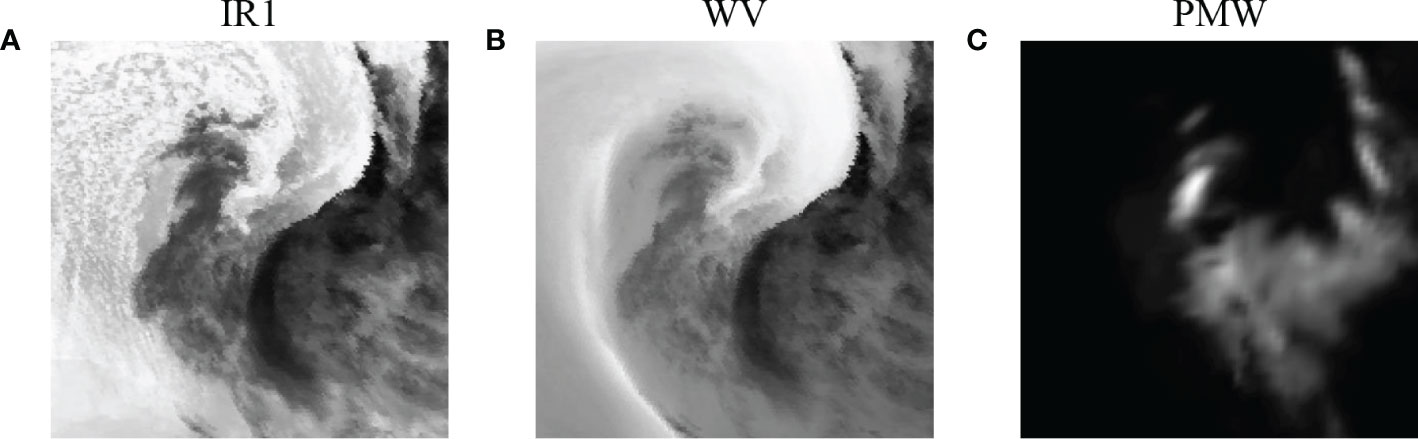
Figure 1 Examples of three channels from TCIR. They are scaled to the range [0, 256) and presented in grayscale.

It should be noted that there were a lot of near-dissipating or immature tropical cyclones in the dataset with size designated as 0, so we selected basin images with TC sizes larger than 0 for this study. Therefore, our final experimental data contain 44,161 frames with three channels of IR1, WV, and PMW per frame.

In the dataset, there exist some damaged values. There are two groups of them, one is NAN values, and another is extremely large values. These damaged values will have a negative impact on the performance of wind radius estimation, so we refer to the method of previous researchers (Chen et al., 2018) to assign the NAN values as 0, and replace the value greater than 1000 with 0. We scaled the image size to 64 × 64 by bilinear interpolation to reduce the computational cost. The dataset was randomly divided into training, validation, and test sets in the ratio of 80:5:15 (Table 1). The training dataset was used to learn the intrinsic association of the images with R34, and the validation dataset was used to find the best super-parameters in the model to obtain the best-performing CNN solution. Finally, the best-performing CNN scheme was applied to the test data for an independent evaluation of its performance.

TABLE 1

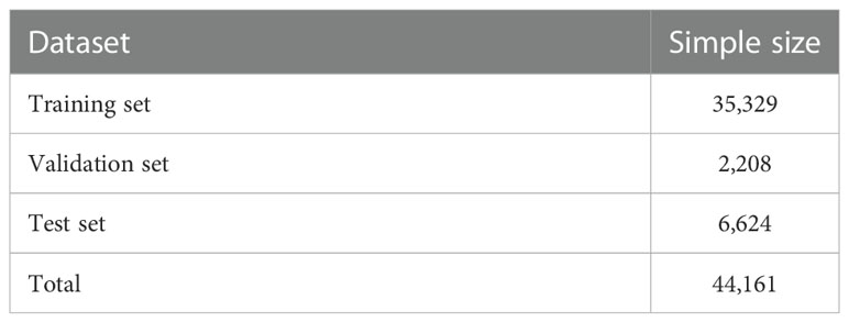
Table 1 Sample data used in the study.

2.2. Problem definitions

Deep learning methods can automatically learn important features related to the target from large amounts of data and establish a relationship between the data and the target (Fei et al., 2022). The proposed deep learning method is designed to discover the intrinsic relationship between the TC image data and R34 to provide accurate R34 estimates. Thus, our problem is a regression problem for image data. Multisource satellite data are inputted into the deep learning model. After several nonlinear operations, the regression result of this image (R34) is outputted (Figure 2).

FIGURE 2

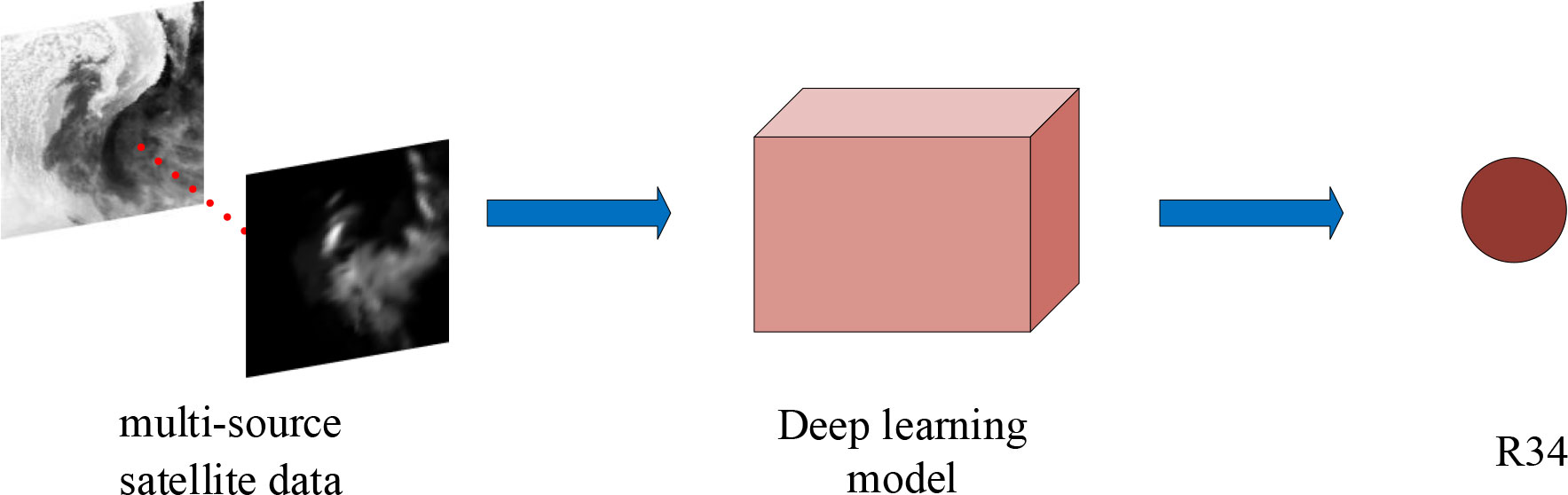
Figure 2 Problem definition framework.

2.3. Architecture of TC-Resnet model

Considering the good performance of the ResNet-50 model in image processing tasks (Ray, 2018; Dong et al., 2020; Walvekar and Shinde, 2020; Torres and Fraternali, 2021; Oerlemans et al., 2022), we chose it as the basic framework for TC-Resnet (Figure 3) and improved it: the Conv-block (Figure 4A) in the standard resnet50 model was replaced with our proposed improved residual block (Figure 4B), and a combined channel–spatial dual attention mechanism (Woo et al., 2018) was applied to our model. TC-Resnet uses three convolution blocks with different convolution layers and filter sizes. The first type of convolution block consists of a convolution layer with a 7 × 7 convolution kernel and a maximum pooling layer. This convolution block acts as the input layer of the model, and the input contains 12,288 (3 × 64 × 64) values. The second type of convolution block consists of three convolution layers with 1 × 1, 3 × 3, and 1 × 1 convolution kernels. Each convolution layer in this convolution block uses a unique number of filters. The third type of convolution block has a two-branch structure that can be used for downsampling according to the input requirements of the model. Each branch of this convolution block consists of three convolution layers; one branch has 1 × 1, 3 × 3, and 1 × 1 convolution kernels, and the other has 1 × 1, 5 × 5, and 1 × 1 convolution kernels. These convolution blocks are stacked in a certain number of repetitions to form the main structure of TC-Resnet for extracting features. The output feature maps are then successively inputted into a channel attention mechanism and a spatial attention mechanism to suppress irrelevant features and enhance the target regions. The computed feature maps are compressed into 2,048 1 × 1 feature maps by applying a global average pooling operation after the attention mechanism. These feature maps are flattened and then fed into the fully connected (FC) layer for wind radius computation.

FIGURE 3

Figure 3 Overall structure of TC-Resnet.

FIGURE 4

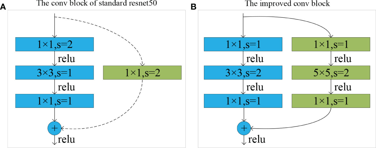
Figure 4 (A) Conv-block of standard resnet-50 and (B) improved residual block. “⊕” denotes add, which is the element-by-element addition of the values. “s” is the acronym for Stride, which indicates the step size when the convolution kernel traverses the feature map.

Padding is applied to all convolution layers to avoid removing features from the outer regions of the TC. “1 × 1, Conv, 64, s = 2” in Figure 3 indicates a convolution operation with a step size of 2 that uses 64 filters with a 1 × 1 convolution kernel. “3 × 3, Pool, 64, s = 2” indicates a maximum pooling operation with a range of 3 × 3 and a step size of 2 for the feature maps. The other expressions follow this naming convention. The dashed sections, namely, X3, X3, X5, and X2, indicate that the corresponding residual structures are repeated 3, 3, 5, and 2 times, respectively. “Avg pool” denotes the average pool, and “Flatten” denotes the conversion of a multidimensional feature to a one-dimensional feature so that it can be fed to the FC layer.

2.3.1. Improvement of residual blocks

If the input and output feature maps of the residual unit are not the same size, then the shortcut branch cannot be directly added to the trunk branch. The Conv-block of the standard ResNet-50 network uses a 1 × 1 convolution kernel with a step size of 2 in the shortcut branch for downsampling to make both feature maps the same size (He et al., 2016) (Figure 4A).

Since the convolution kernel width (kernel = 1) is smaller than the step size (s = 2), it cannot traverse all the feature information in the feature map. Only the information in the red boxed part of Figure 5A can be passed to the next layer. None of the information in the nonboxed part is involved in the convolution calculation; thus, 3/4 of the information is missing, and some fine features in the data are not captured. For neighboring time-node cloud systems with small feature differences, such missing information prevents the model from extracting deeper spatial pixel information, thereby reducing recognition accuracy. The 1 × 1 convolution kernel of the shortcut branch can reduce dimensionality by linearly combining information from different channels but cannot extract feature information, thus decreasing the utilization of the shortcut branch. Therefore, we improved the convolution block by adding one 1 × 1, stride = 1 convolution layer to the shortcut branch for up-dimensioning and a 5 × 5, stride = 2 convolution layer for spatial and channel feature extraction (Figure 4B). The original downsampling process of the shortcut branch was transferred to the new 5 × 5 convolution layer, and the large convolution kernel can traverse all the information of the feature map, hence solving the information loss issue of the original model (Figure 5B). The ReLu activation function was then introduced to enhance nonlinear fitting.

FIGURE 5

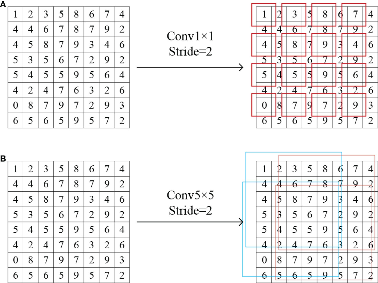
Figure 5 (A) Feature information traversal before improvement and (B) feature information traversal after improvement.

2.3.2. Integration of attention mechanism

The complex atmospheric factors during typhoon formation make features within the cloud spiral radius obscure (Zhou et al., 2020), which makes wind radius estimation difficult. We introduced CBAM into TC-Resnet, so that the model could actively learn to focus on the contours of the target wind radius in an image while suppressing irrelevant background regions for excellent wind radius estimation. The CBAM attention module combines the spatial and channel dimensions (Figure 6). Compared with SENet, CBAM can achieve better results because the latter uses an attention mechanism that focuses on the channel only (Hu et al., 2018; Chen et al., 2021).

FIGURE 6

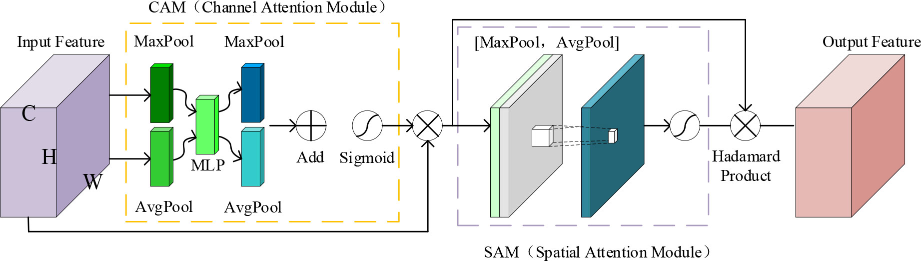
Figure 6 Structure of the CBAM. The left part represents the channel attention module and the right part represents the spatial attention module. The feature map passes first through the left part and then through the right part.

CBAM is implementated as follows.

The first step is to generate the channel attention map. Global maximum pooling and global average pooling are performed on the input feature map F in the HW direction respectively, and the information in the HW direction is aggregated into two C × 1 × 1 vectors, which are then passed to a multilayer perceptron MLP for calculation respectively. Both share the weight values of the MLP, and the results of the two calculations are summed to regenerate a C × 1 × 1 vector. The sigmoid function is applied to this regenerated vector to generate the channel attention map. This process is expressed as follows:

$$C\left(F\right)= Sigmoid\left(MLP\left(Maxpool\left(F\right)\right)+MLP\left(Avgpool\left(F\right)\right)\right)$$

Next, the spatial attention map is generated. F first performs global maximum pooling and global average pooling in the direction of channel C to generate two 1 × H × W feature maps. The two feature maps are spliced in the channel dimension to obtain a 2 × H × W feature map, which is then convolved to generate a 1 × H × W feature map. Finally, the sigmoid function is applied to generate the spatial attention map. This process is expressed as follows:

$$S\left(F\right)=Sigmoid\left(Conv\left(Concat\left(Maxpool\left(F\right),Avgpool\left(F\right)\right)\right)\right)$$

where Conv represents the convolution operation applied to the feature map and Concat represents that two feature maps are concatenated together in the channel direction.

The overall operation process of CBAM can be expressed as follows:

$$\{\begin{array}{c}{F}^{\prime }=C\left(F\right)\otimes F\\ F^{″}=S\left(F^{\prime }\right)\otimes F^{\prime }\end{array}$$

where ⊗ represents the Hadamard product, F′ is the intermediate variable of the feature map F passing through the channel attention module, and F″ represents the output passing through the spatial attention module.

CBAM combines channel and spatial attention mechanisms sequentially, thereby effectively improving the extraction of key features from the feature maps and suppressing unnecessary features. The channel attention mechanism automatically calculates the weight of each channel feature map so that the model learns to focus on the key information channels that contain considerable weight. The spatial attention mechanism can calculate the importance of each region of the image. Thus, the model learns to filter out unimportant background noise information and enhance the feature regions of the target to obtain critical features. The application of CBAM to wind radius estimation can enhance the model’s ability to extract key features from TC cloud maps and improve its wind radius estimation performance.

2.4. Model validation and optimization

We use the Pearson correlation coefficient (R) and Mean absolute error (MAE) to evaluate model performance.

MAE: the average of the distance between the model-prediction (R34 estimation) and the sample’s true value (Best-track R34). MAE can be defined as:

$$MAE=\frac{1}{n}\sum _{i=1}^n\left|\left(\widehat{y_i}-y_i\right)\right|$$

where n is the number of samples, $\widehat{y_i}$ is the R34 estimation, and y_i is the true value (Best-track R34).

R: the quotient of the covariance and standard deviation between two variables (R34 estimation and Best-track R34). R can be defined as:

$$R=\frac{{\sum }_{i=1}^n\left(y_i-\overline{y_i}\right)\left(\widehat{y_i}-\overline{\widehat{y_i}}\right)}{\sqrt{{\sum }_{i=1}^n{\left(y_i-\overline{y_i}\right)}^2}\sqrt{{\sum }_{i=1}^n{\left(\widehat{y_i}-\overline{\widehat{y_i}}\right)}^2}}$$

where n is the number of samples, $\widehat{y_i}$ is the R34 estimation, and y_i is the Best-track R34.

For the optimizer, adaptive moment estimation (Adam) is used because this optimizer is commonly adopted and properly considers the direction and learning rate to find the optimal loss (Nair and Hinton, 2010; Kingma and Ba, 2014).

Comparison of model performance: We compare several deep learning models commonly used in image processing, namely, ResNet-18 (He et al., 2016), ResNet-50 (He et al., 2016), VGGNet (Simonyan and Zisserman, 2014), and GoogLeNet (Szegedy et al., 2015), on the same dataset to evaluate the performance of our model.

The size of the convolution kernel in each layer is sensitive to the characteristics of the input data. The smaller the convolution kernel, the better the model can capture the local features of the input image. Large convolution kernels are suitable for acquiring the general pattern of the input image (Li et al., 2017). Therefore, the optimal convolution kernel size suitable for the characteristics of satellite TC images should be determined. Therefore, we experimented with the size of the convolution kernel of the downsampled convolution layer in the modified residual block to select the size (from 3 to 9, with increments of 2) that best fits TC image characteristics.

3. Results and discussion

The model was trained using the CUDA-enabled PyTorch framework (Python). After testing different learning rates, we finally determined the learning rate to be 0.0001. For epoch selection, we used the early stop strategy, which is a method of informing when to stop running the iterative algorithm during training to improve the overall performance of the CNN model by reducing model overfitting (Raskutti et al., 2014). The validation loss is the model error of the validation data from a specified loss function, which tells the CNN model when to stop training. In the training process of this study, we set the iteration period to 20 epochs, and the model training process was stopped when the validation loss stopped decreasing within a certain period (Figure 7).

FIGURE 7

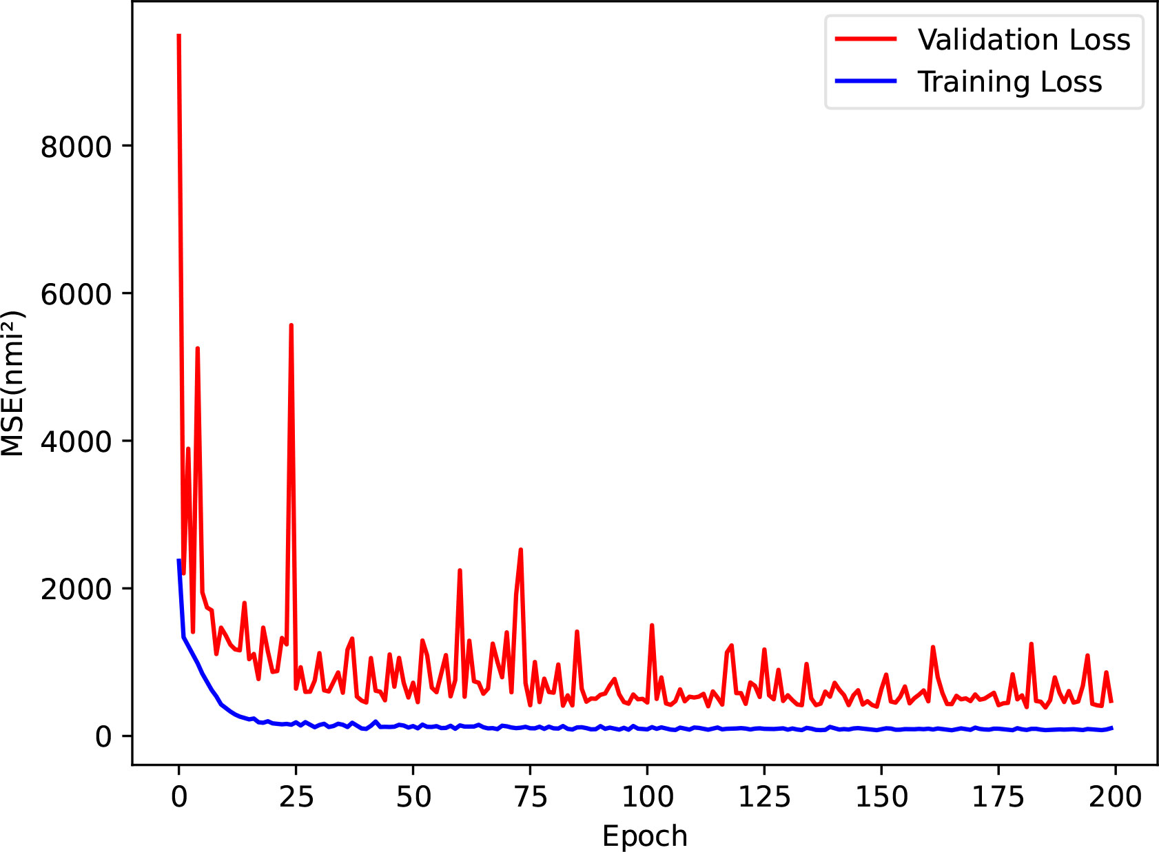
Figure 7 Plot of the decreasing loss values of the model on the training and validation sets. An epoch indicates that all training samples are computed in the model once in full and MSE indicates mean squared error.

3.1. Test on independent datasets

We used 2,208 (validation) and 6,624 (test) satellite images to analyze the performance of TC-Resnet. The optimal-parameter-based TC-Resnet model configuration on the validation set yields MAE and R values of 10.958 nmi and 0.918, respectively, in R34 estimation (Figure 8A). MAE and R values of 11.287 nmi and 0.907, respectively, are obtained from the model application to the test dataset (Figure 8B). The scatterplots in Figure 8 suggest that our results fit well; the R34 estimates obtained from our model are highly correlated with the Best-track R34, although there are some outliers. Both the validation and test sets contain peculiar outliers (in the red boxes in Figure 8); this anomalous part shows that the model gives estimates of around 210 nmi regardless of the true wind radius. This is because some of the images in our dataset had large numbers of missing values and unusually large values; in some cases, the entire image was empty. To investigate the robustness of our model to large quantities of missing values and outliers, we did not remove them. Instead, we simply set them to 0. After this method, TC images with a small number of damaged values can still get good R34 estimates by the calculation of our model, and these weakened images also make the model enhanced to handle low-quality images. It is worth noting that some images with a large number of damaged values have considerable similarity after such processing, so the model can easily mistake them for the same type of TC images and predict very close R34 values (about 210 nmi) for them. These close R34 values depend on the distribution of anomalous data in the satellite data and vary with the data, so we did not set a specific threshold in the model to attenuate the side effects of the damaged data because this threshold is difficult to determine. This type of anomalous image is a very low percentage of the dataset, only about 1%, so we allowed it to exist. The fact that the test set had more data than the validation set (red boxes) is the reason the test set has weaker results than the validation set.

FIGURE 8

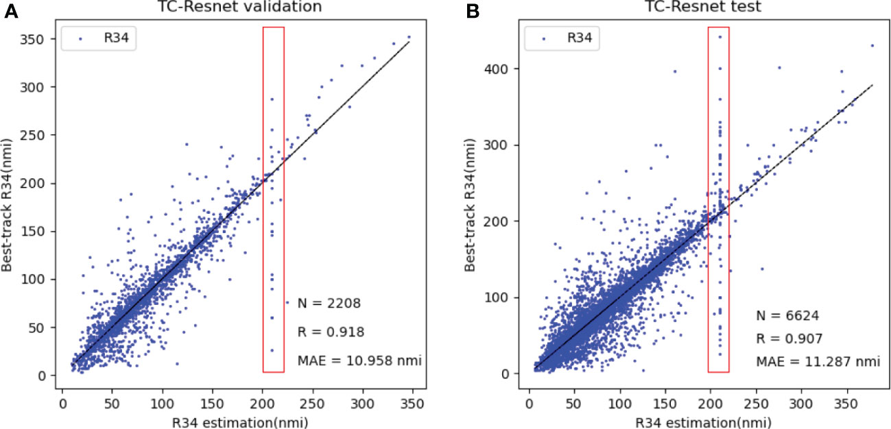
Figure 8 Scatter plot of model results on the (A) validation and (B) test sets.

As shown in Figure 9, we examined 60 predictions randomly selected from the test set, whose MAE and R were 8.675 nmi and 0.923, respectively, which were similar to the evaluation indicators of the whole independent test set. The predicted values fit well with the actual values for most points, which indicates that our deep learning model performs well on the independent dataset.

FIGURE 9

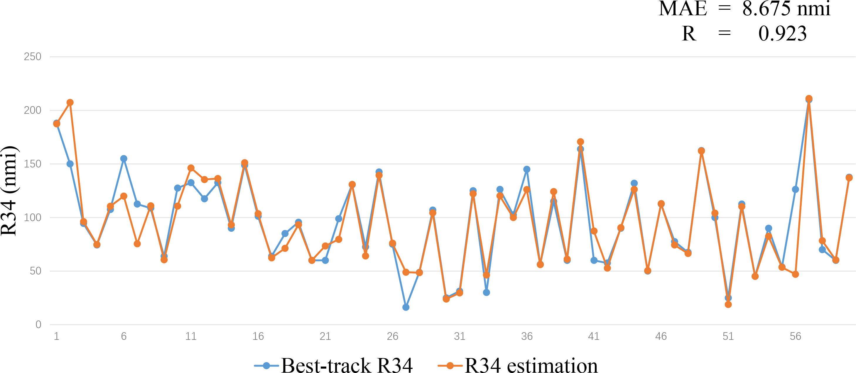
Figure 9 Comparison of predicted results and labeled values for 60 randomly selected test sets.

3.2. Sensitivity experiment of data sources

Researchers mainly use infrared satellite data in TC size studies because their high resolution reveals substantial observational information. Nonetheless, despite the low resolution of microwave satellite data, they can penetrate most clouds beyond the top layer, which is a beneficial feature when a central dense overcast exists (Demuth et al., 2004) and play a crucial role in revealing convective organization and eyewall structure (Xiang et al., 2019; Hawkins et al., 2001; Wimmers and Velden, 2010). Therefore, we investigated the effect of data sources on wind radius estimates. The experimental results are shown in Figure 10. In wind radius estimation, the MAE values of the R34 estimation errors based on IR1, WV, and PMW channel data are 15.266 nmi, 13.751 nmi, and 17.882 nmi, respectively, when only single-channel data are considered, which shows that the infrared data perform significantly better than the microwave data. When considering the dual-channel data for wind radius estimation, the performance of the WV and PMW dual-channel data (MAE=11.684 nmi) is significantly better than that of the IR1 and WV dual-channel data (MAE=12.357 nmi) and the IR1 and PMW dual-channel data (MAE=13.254 nmi). We found that the WV channel and PMW channel each seem to have more complementary information about the wind radius features. Wind radius estimation was further improved by adding IR1 channel data to the combined WV and PMW channel data. Findings show that the combined use of infrared and microwave data provides more valid features about wind radii than single-channel infrared data and single-channel microwave data in wind radius estimation. The wind radius estimation results obtained from the use of multisource data (combined infrared and microwave data) are better by about 26% than those from the use of infrared data alone, which is the common practice.

FIGURE 10

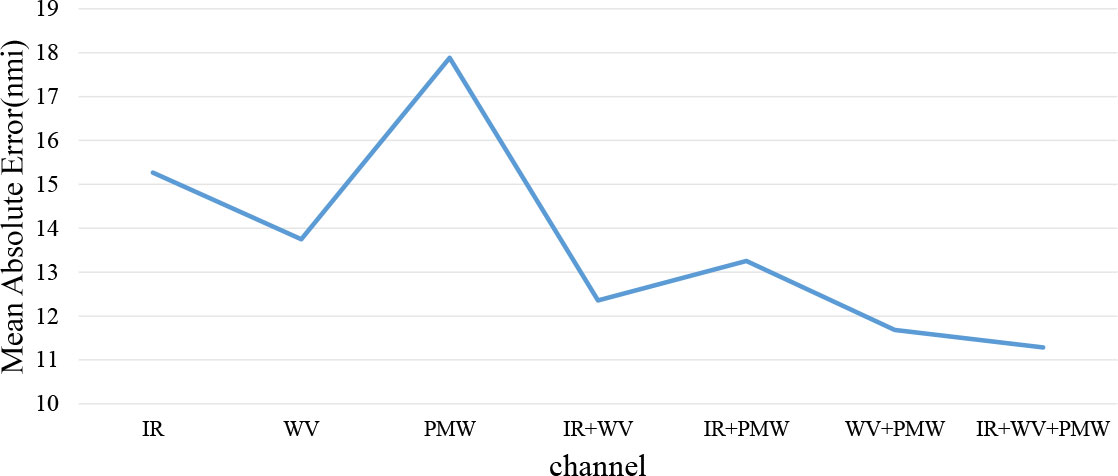
Figure 10 Performance of different channels of satellite data and their combinations.

3.3. Determination of optimal model parameters

In improving the convolution block, we configured the appropriate convolution kernel size for the downsampling layer to avoid information loss and optimize the model. As shown in Figure 11, the configuration of different convolution kernel sizes significantly affects the wind radius estimation performance of the model. In the validation dataset, the improved model does not totally outperform the standard ResNet-50; only the 3 × 3 and 5 × 5 convolution kernel configurations perform better, indicating that the model is sensitive to the convolution kernel size. When the convolution kernel size is 5 × 5, the model obtains MAE and R values of 11.375 nmi and 0.907, respectively. The wind radius estimation performance is better compared with that under the three other convolution kernel sizes. This may be because a smaller convolution kernel loses some important information due to the step size (s = 2), whereas a larger convolution kernel does not capture local features well.

FIGURE 11

Figure 11 Scatterplot of different parameter settings on validation set. (A) Unimproved residual blocks, (B) with added 3 × 3 convolution kernel, (C) with added 5 × 5 convolution kernel, (D) with added 7 × 7 convolution kernel, and (E) with added 9 × 9 convolution kernel. In each figure, the horizontal axis is the R34 estimation of the model output, the vertical axis is the corresponding label, and the bottom-right corner shows the N, R, and MAE values.

To explore whether reducing the background noise of the TC cloud system by the attention mechanism can improve the wind radius estimation results, we added CBAM behind the last convolution layer. And we tested the model with different configurations after introducing the attention mechanism and made the scatterplot in Figure 12. By comparing Figure 11, 12, it can be found that after reducing the background noise of the TC cloud system, the performance of the Resnet-50 model, the 5×5 convolution kernel configuration, the 7×7 convolution kernel configuration, and the 9×9 convolution kernel configuration show 2.46%, 3.66%, 3.74%, and 2.31% improvement in the R34 estimation task, respectively, and only the performance of the model with the 3×3 convolution kernel configuration decreases by 0.83%. Accordingly, we believe that not every model can effectively reduce the background noise of the TC cloud system and thus optimize the R34 estimation with the help of the attention mechanism. However, the attention mechanism can suppress the image background noise well in most cases to achieve better operational performance. Based on the test results, we chose a model with a 5×5 convolutional kernel configuration embedded with an attention mechanism as our final operational model. This model is able to fully capture the important detailed features of the TC cloud system as well as reduce the background noise of the TC cloud system to achieve better performance.

FIGURE 12

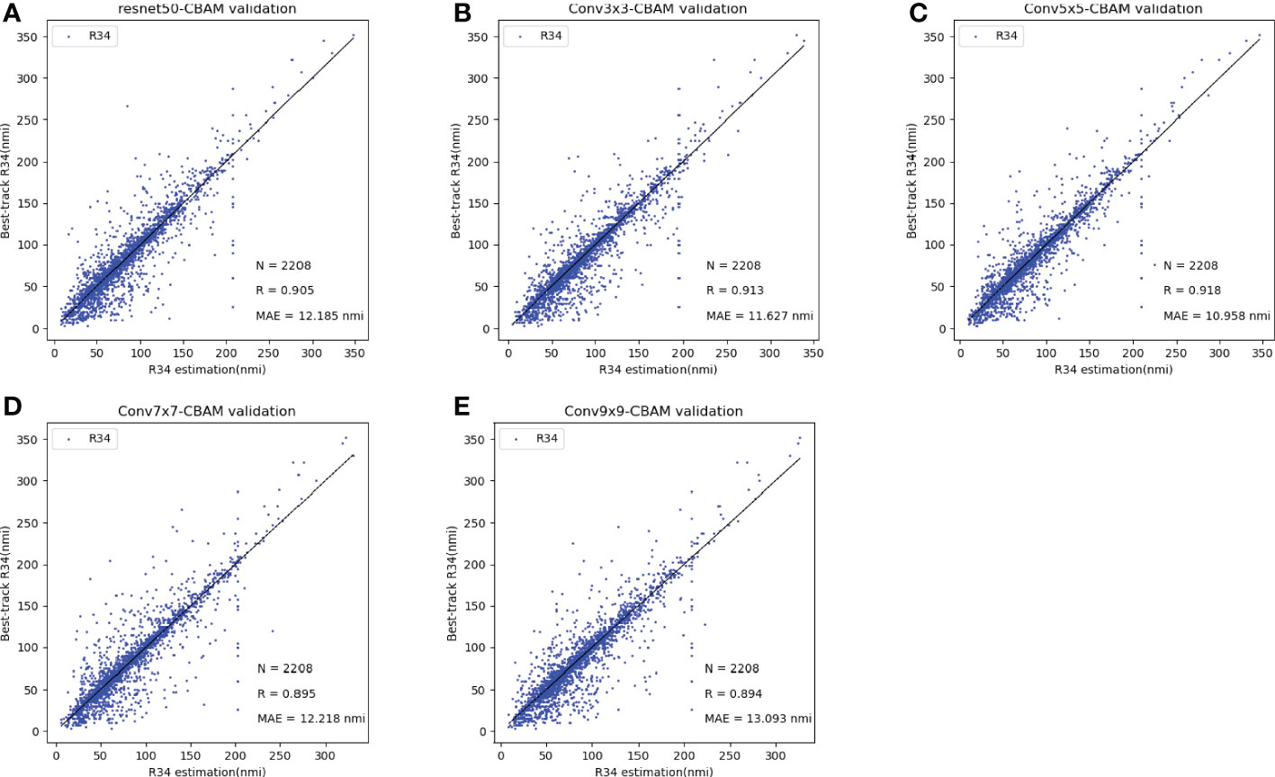
Figure 12 Scatterplot of results obtained after incorporation of attention mechanism (CBAM) based on Figure 11. (A) Unimproved residual blocks, (B) with added 3 × 3 convolution kernel, (C) with added 5 × 5 convolution kernel, (D) with added 7 × 7 convolution kernel, and (E) with added 9 × 9 convolution kernel. In each figure, the horizontal axis is the R34 estimation of the model output, the vertical axis is the corresponding label, and the bottom-right corner shows the N, R, and MAE values. .

3.4. Comparison with other deep learning models and previous studies

We evaluated several widely used deep learning models on the same dataset and compared the performance of TC-Resnet with previous research results (Table 2). Among these commonly used deep learning models, the ResNet-50 model performs the best, with MAE and R values of 12.788 nmi and 0.892, respectively. However, the performance of TC-Resnet, with MAE and R values of 11.287 nmi and 0.907, respectively, is better by 11.73% compared with that of ResNet-50. Our model also performs excellently compared with previous models. However, a direct quantitative comparison with previous research results was difficult because of the studies’ differences in study periods and regions. Nonetheless, we used TC data with the longest period (2003–2017) and the most comprehensive spatial coverage (global), yet our R34 estimation performance is better compared with that of the other operational products. Therefore, the proposed method should be an effective tool for TC size estimation.

TABLE 2

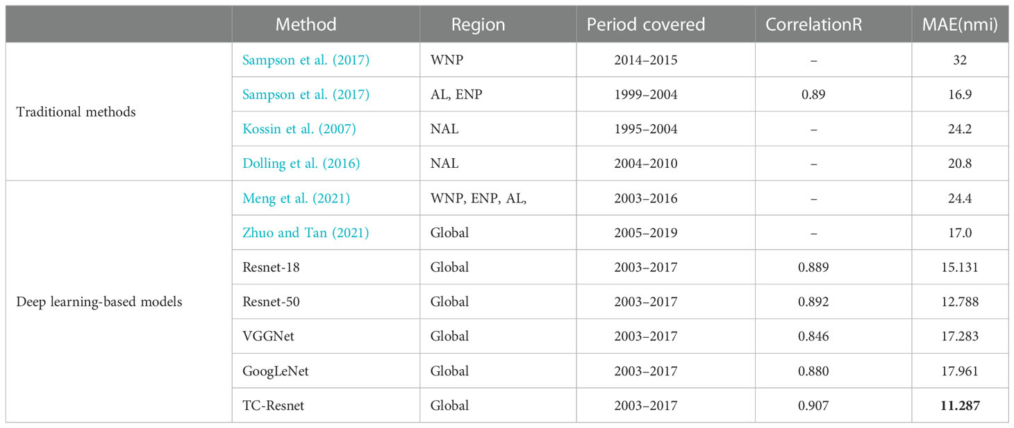
Table 2 Comparison of TC size estimation models in terms of correlation and MAE. WNP: western north Pacific; ENP: eastern north Pacific; NAL: north Atlantic.

4. Conclusions

This study proposes TC-Resnet, a deep CNN model that automatically estimates wind radii based on combined infrared and microwave satellite data. In light of the considerable blurring and background noise in TC cloud systems, we introduced CBAM to suppress such background noise while enhancing target features and improved the traditional residual structure to enhance the model’s ability to capture detailed features. We trained, validated, and independently tested TC-Resnet, and the results show that our method, which does not require specialized domain knowledge or manual operation, is easy to operate and outperforms traditional methods. Our method also performs better than widely used deep learning–based methods. Thus, TC-Resnet can obtain vital information about wind radius features.

To our knowledge, this study is the first to estimate R34 using a deep learning model that combines infrared and microwave satellite data. In previous studies, although microwave data were considered suitable for investigating TC structures, their low spatial resolution limited their application. Current deep learning–based methods of R34 estimation focus only on infrared satellite data; they ignore the applicability of microwave data to wind radius estimation. According to the results of the current study, in R34 estimation, the use of combined infrared and microwave satellite data outperforms the use of microwave or infrared satellite data alone. The use of such combined data produces a performance improvement of about 26% compared with the use of infrared data alone. Therefore, this new method can be a powerful tool for TC size estimation.

In this study, infrared and microwave satellite data were used to estimate wind radii. Although satisfactory results were obtained, the possibility of optimizing the model by adding other environmental data, such as wind field data, needs further study. In addition, according to JTWC data, tropical cyclones usually have asymmetric wind fields. Lu et al. (2011) found that larger radii are usually found in the northeast quadrant, followed by the southeast and southwest quadrants. However, this study only used the average of 34kt wind radii in the four quadrants and did not consider the asymmetric situation of tropical cyclones due to low-level environments, such as enhanced cross equatorial flow and low/mid-level relative humidity (Mohapatra and Sharma, 2015). The study of tropical cyclone asymmetries is important for more accurate predictions of TC-related hazardous areas, which is a priority for future research.

Data availability statement

The original contributions presented in the study are included in the article/Supplementary Material. Further inquiries can be directed to the corresponding authors.

Author contributions

JX and XW developed the idea. JX designed the research, analyzed the data, and wrote the manuscript. XW and HaW guided the whole study and revised the manuscript. CZ, HuW, and JZ contributed significantly to the text. All authors contributed to the article and approved the submitted version.

Funding

This research is partially supported by the National Natural Science Foundation of China (Grant No. 61802424), the National Natural Science Foundation of China (Grant No. 42276205) and the Natural Science Foundation of Shandong Province (Grant No. ZR2021MD068)

Acknowledgments

Special thanks to the Institute of Numerical Meteorology and Oceanography, College of Meteorology and Oceanography, National University of Defense Technology for the equipment support.

Conflict of interest

The authors declare that the research was conducted in the absence of any commercial or financial relationships that could be construed as a potential conflict of interest.

Publisher’s note

All claims expressed in this article are solely those of the authors and do not necessarily represent those of their affiliated organizations, or those of the publisher, the editors and the reviewers. Any product that may be evaluated in this article, or claim that may be made by its manufacturer, is not guaranteed or endorsed by the publisher.

References

Baek Y. H., Moon I. J., Im J., Lee J. (2022). A novel tropical cyclone size estimation model based on a convolutional neural network using geostationary satellite imagery. Remote Sens. 14 (2), 426. doi: 10.3390/rs14020426

CrossRef Full Text | Google Scholar

Bessho K., DeMaria M., Knaff J. A. (2006). Tropical cyclone wind Retrievals from the advanced microwave sounding unit: Application to surface wind analysis. J. Appl. Meteorology Climatology 45, 3, 399–415. doi: 10.1175/JAM2352.1

CrossRef Full Text | Google Scholar

Cha E. J., Knutson T. R., Lee T. C., Ying M., Nakaegawa T. (2020). Third assessment on impacts of climate change on tropical cyclones in the typhoon committee region–part II: Future projections. Trop. Cyclone Res. Rev. 9 (2), 75–86. doi: 10.1016/j.tcrr.2020.04.005

CrossRef Full Text | Google Scholar

Chavas D. R., Lin N., Emanuel K. (2015). A model for the complete radial structure of the tropical cyclone wind field. part I: Comparison with observed structure. J. Atmospheric Sci. 72 (9), 3647–3662. doi: 10.1175/JAS-D-15-0014.1

CrossRef Full Text | Google Scholar

Chen B., Chen B. F., Lin H. T. (2018). “Rotation-blended CNNs on a new open dataset for tropical cyclone image-to-intensity regression,” in Proceedings of the 24th ACM SIGKDD international conference on knowledge discovery & data mining. (New York: Assoc Computing Machinery), 90–99.

Google Scholar

Chen L., Tian X., Chai G., Zhang X., Chen E. (2021). A new CBAM-P-Net model for few-shot forest species classification using airborne hyperspectral images. Remote Sens. 13 (7), 1269. doi: 10.3390/rs13071269

CrossRef Full Text | Google Scholar

Chen R., Wang X., Zhang W., Zhu X., Li A., Yang C. (2019). A hybrid CNN-LSTM model for typhoon formation forecasting. GeoInformatica 23 (3), 375–396. doi: 10.1007/s10707-019-00355-0

CrossRef Full Text | Google Scholar

Chen R., Zhang W., Wang X. (2020). Machine learning in tropical cyclone forecast modeling: A review. Atmosphere 11 (7), 676. doi: 10.3390/atmos11070676

CrossRef Full Text | Google Scholar

DeMaria M., Knaff J. A., Brennan M. J., Brown D., Knabb R. D., DeMaria R. T., et al. (2013). Improvements to the operational tropical cyclone wind speed probability model. Weather Forecasting 28 3, 586–602. doi: 10.1175/WAF-D-12-00116.1

CrossRef Full Text | Google Scholar

Demuth J. L., DeMaria M., Knaff J. A. (2006). Improvement of advanced microwave sounding unit tropical cyclone intensity and size estimation algorithms. J. Appl. Meteorology Climatology 45 (11), 1573–1581. doi: 10.1175/JAM2429.1

CrossRef Full Text | Google Scholar

Demuth J. L., DeMaria M., Knaff J. A., Vonder Haar T. H. (2004). Evaluation of advanced microwave sounding unit tropical-cyclone intensity and size estimation algorithms. J. Appl. Meteorology 43 2, 282–296. doi: 10.1175/1520-0450(2004)043<0282:EOAMSU>2.0.CO;2

CrossRef Full Text | Google Scholar

Dolling K., Ritchie E. A., Tyo J. S. (2016). The use of the deviation angle variance technique on geostationary satellite imagery to estimate tropical cyclone size parameters. Weather Forecasting 31 (5), 1625–1642. doi: 10.1175/WAF-D-16-0056.1

CrossRef Full Text | Google Scholar

Dong R., Xu D., Jiao L., Zhao J., An J. (2020). A fast deep perception network for remote sensing scene classification. Remote Sens. 12 (4), 729. doi: 10.3390/rs12040729

CrossRef Full Text | Google Scholar

Fei T., Huang B., Wang X., Zhu J., Chen Y., Wang H., et al. (2022). A hybrid deep learning model for the bias correction of SST numerical forecast products using satellite data. Remote Sens. 14 (6), 1339. doi: 10.3390/rs14061339

CrossRef Full Text | Google Scholar

Hawkins J. D., Lee T., Turk F., Richardson K., Sampson C., Kent J. (2001). Mapping tropical cyclone characteristics via passive microwave remote sensing. In Proceedings of the 11th Conference on Satellite Meteorology and Oceanography, Madison, WI, USA, 15–18.

Google Scholar

He K., Zhang X., Ren S., Sun J. (2016). “Deep residual learning for image recognition,” in Proceedings of the IEEE conference on computer vision and pattern recognition. (New York: IEEE), 770–778.

Google Scholar

Hu J., Shen L., Sun G. (2018). “Squeeze-and-excitation networks,” in Proceedings of the IEEE conference on computer vision and pattern recognition. (New York: IEEE), 7132–7141.

Google Scholar

Joyce R. J., Janowiak J. E., Arkin P. A., Xie P. (2004). CMORPH: A method that produces global precipitation estimates from passive microwave and infrared data at high spatial and temporal resolution. J. Hydrometeorology 5 (3), 487–503. doi: 10.1175/1525-7541(2004)005<0487:CAMTPG>2.0.CO;2

CrossRef Full Text | Google Scholar

Kim H. J., Moon I. J., Oh I. (2022). Comparison of tropical cyclone wind radius estimates between the KMA, RSMC Tokyo, and JTWC. Asia-pacific J Atmospheric Sci. 58, 563–576. doi: 10.1007/s13143-022-00274-5

CrossRef Full Text | Google Scholar

Kingma D. P., Ba J. (2014). Adam: A method for stochastic optimization. arXiv preprint arXiv 1412, 6980. doi: 10.48550/arXiv.1412.6980

CrossRef Full Text | Google Scholar

Knaff J. A., Sampson C. R. (2015). After a decade are Atlantic tropical cyclone gale force wind radii forecasts now skillful? Weather Forecasting 30 (3), 702–709. doi: 10.1175/WAF-D-14-00149.1

CrossRef Full Text | Google Scholar

Knaff J. A., Sampson C. R., Chirokova G. (2017). A global statistical–dynamical tropical cyclone wind radii forecast scheme. Weather Forecasting 32 (2), 629–644. doi: 10.1175/WAF-D-16-0168.1

CrossRef Full Text | Google Scholar

Knaff J. A., Slocum C. J., Musgrave K. D., Sampson C. R., Strahl B. R. (2016). Using routinely available information to estimate tropical cyclone wind structure. Monthly Weather Rev. 144, 1233–1247. doi: 10.1175/MWR-D-15-0267.1

CrossRef Full Text | Google Scholar

Knapp K. R., Ansari S., Bain C. L., Bourassa M. A., Dickinson M. J., Funk C., et al. (2011). Globally gridded satellite observations for climate studies. Bull. Am. Meteorological Soc. 92 (7), 893–907. doi: 10.1175/2011BAMS3039.1

CrossRef Full Text | Google Scholar

Kossin J. P., Knaff J. A., Berger H. I., Herndon D. C., Cram T. A., Velden C. S., et al. (2007). Estimating hurricane wind structure in the absence of aircraft reconnaissance. Weather Forecasting 22 1, 89–101. doi: 10.1175/WAF985.1

CrossRef Full Text | Google Scholar

Kurihara Y., Bender M. A., Ross R. J. (1993). An initialization scheme of hurricane models by vortex specification. Monthly Weather Rev. 121 (7), 2030–2045. doi: 10.1175/1520-0493(1993)121<2030:AISOHM>2.0.CO;2

CrossRef Full Text | Google Scholar

Landsea C. W., Franklin J. L. (2013). Atlantic Hurricane database uncertainty and presentation of a new database format. Monthly Weather Rev. 141 (10), 3576–3592. doi: 10.1175/MWR-D-12-00254.1

CrossRef Full Text | Google Scholar

Lee J., Im J., Cha D. H., Park H., Sim S. (2019). Tropical cyclone intensity estimation using multi-dimensional convolutional neural networks from geostationary satellite data. Remote Sens. 12 (1), 108. doi: 10.3390/rs12010108

CrossRef Full Text | Google Scholar

Lee Y. K., Kwon M. (2015). An estimation of the of tropical cyclone size using COMS infrared imagery. Atmosphere 25 (3), 569–573. doi: 10.14191/Atmos.2015.25.3.569

CrossRef Full Text | Google Scholar

Li L., Jamieson K., DeSalvo G., Rostamizadeh A., Talwalkar A. (2017). Hyperband: A novel bandit-based approach to hyperparameter optimization. J. Mach. Learn. Res. 18, 6765–6816. doi: 10.48550/arXiv.1603.06560

CrossRef Full Text | Google Scholar

Lu X., Yu H., Lei X. (2011). Statistics for size and radial wind profile of tropical cyclones in the western north pacific. Acta Meteorol Sin. 25, 104–112. doi: 10.1007/s13351-011-0008-9

CrossRef Full Text | Google Scholar

Meng F., Xie P., Li Y., Sun H., Xu D., Song T. (2021). “Tropical cyclone size estimation using deep convolutional neural network,” in 2021 IEEE international geoscience and remote sensing symposium IGARSS. (New York: IEEE), 8472–8475.

Google Scholar

Miller J., Maskey M., Berendes T. (2017). “Using deep learning for tropical cyclone intensity estimation,” in AGU fall meeting abstracts. Washington: Amer Geophysical Union, vol. 2017. IN11E–IN105.

Google Scholar

Mohapatra M., Sharma M. (2015). Characteristics of surface wind structure of tropical cyclones over the north Indian ocean. J. Earth Syst. Sci. 124, 1573–1598. doi: 10.1007/s12040-015-0613-6

CrossRef Full Text | Google Scholar

Mueller K. J., DeMaria M., Knaff J., Kossin J. P., Vonder Haar T. H. (2006). Objective estimation of tropical cyclone wind structure from infrared satellite data. Weather Forecasting 21 (6), 990–1005. doi: 10.1175/WAF955.1

CrossRef Full Text | Google Scholar

Nair V., Hinton G. E. (2010). “Rectified linear units improve restricted boltzmann machines,” in Icml. New York: Assoc Computing Machinery.

Google Scholar

NHC. (2016). Introduction to storm surge. Natl. Hurricane Center/Storm Surge Unit. pp. 5. Available at: http://www.nhc.noaa.gov/surge/surge_intro.pdf.

Google Scholar

Oerlemans S. C., Nijland W., Ellenson A. N., Price T. D. (2022). Image-based classification of double-barred beach states using a Convolutional neural network and transfer learning. Remote Sens. 14 (19), 4686. doi: 10.3390/rs14194686

CrossRef Full Text | Google Scholar

Pradhan R., Aygun R. S., Maskey M., Ramachandran R., Cecil D. J. (2017). Tropical cyclone intensity estimation using a deep convolutional neural network. IEEE Trans. Image Process. 27 (2), 692–702. doi: 10.1109/TIP.2017.2766358

CrossRef Full Text | Google Scholar

Quiring S., Schumacher A., Guikema S. (2014). Incorporating hurricane forecast uncertainty into decision support applications. Bull. Amer. Meteor. Soc 95, 47–58. doi: 10.1175/BAMS-D-12-00012.1

CrossRef Full Text | Google Scholar

Raskutti G., Wainwright M. J., Yu B. (2014). Early stopping and non-parametric regression: An optimal data-dependent stopping rule. J. Mach. Learn. Res. 15, 335–366. doi: 10.48550/arXiv.1306.3574

CrossRef Full Text | Google Scholar

Ray S. (2018). Disease classification within dermascopic images using features extracted by resnet50 and classification through deep forest. arXiv preprint arXiv 1807, 05711. doi: 10.48550/arXiv.1807.05711

CrossRef Full Text | Google Scholar

Sampson C. R., Fukada E. M., Knaff J. A., Strahl B. R., Brennan M. J., Marchok T. (2017). Tropical cyclone gale wind radii estimates for the Western north pacific. Weather Forecasting 32 (3), 1029–1040. doi: 10.1175/WAF-D-16-0196.1

CrossRef Full Text | Google Scholar

Sampson C. R., Goerss J. S., Knaff J. A., Strahl B. R., Fukada E. M., Serra E. A. (2018). Tropical cyclone gale wind radii estimates, forecasts, and error forecasts for the western north pacific. Weather Forecasting 33, 1081–1092. doi: 10.1175/WAF-D-17-0153.1

CrossRef Full Text | Google Scholar

Simonyan K., Zisserman A. (2014). Very deep convolutional networks for large-scale image recognition. arXiv preprint arXiv 1409, 1556. doi: 10.48550/arXiv.1409.1556

CrossRef Full Text | Google Scholar

Stark C., Ritchie E. A., Tyo J. S. (2019). “Modelling tropical cyclone wind radii in the Australian region using the deviation angle variance technique,” in IGARSS 2019-2019 IEEE international geoscience and remote sensing symposium. New York: IEEE, 9342–9345.

Google Scholar

Szegedy C., Liu W., Jia Y., Sermanet P., Reed S., Anguelov D., et al. (2015). “Going deeper with convolutions,” in Proceedings of the IEEE conference on computer vision and pattern recognition. (New York: IEEE), 1–9.

Google Scholar

Tallapragada V., and Coauthors (2016). Hurricane weather research and forecasting (HWRF) model: 2015 scientific documentation, august 2015 – HWRF v3.7a. NCAR Dev. Testbed Center Boulder CO, 123. doi: 10.5065/D6ZP44B5

CrossRef Full Text | Google Scholar

Torres R. N., Fraternali P. (2021). Learning to identify illegal landfills through scene classification in aerial images. Remote Sens. 13 (22), 4520. doi: 10.3390/rs13224520

CrossRef Full Text | Google Scholar

Walvekar S., Shinde D. (2020). “Detection of COVID-19 from CT images using resnet50,” in 2nd international conference on communication & information processing (New York: ICCIP).

Google Scholar

Wimmers A. J., Velden C. S. (2010). Objectively determining the rotational center of tropical cyclones in passive microwave satellite imagery. J. Appl. Meteorol. Climatol. 49, 2013–2034.

Google Scholar

Woo S., Park J., Lee J. Y., Kweon I. S. (2018). “Cbam: Convolutional block attention module,” in Proceedings of the European conference on computer vision (Germany: ECCV), pp. 3–19.

Google Scholar

Xiang K., Yang X., Zhang M., Li Z., Kong F. (2019). Objective Estimation of Tropical Cyclone Intensity from Active and Passive Microwave Remote Sensing Observations in the Northwestern Pacific Ocean. Remote Sens. 11, 627. doi: 10.3390/rs11060627

CrossRef Full Text | Google Scholar

Zhang R., Liu Q., Hang R. (2019). Tropical cyclone intensity estimation using two-branch convolutional neural network from infrared and water vapor images. IEEE Trans. Geosci. Remote Sens. 58 (1), 586–597. doi: 10.1109/TGRS.2019.2938204

CrossRef Full Text | Google Scholar

Zhou J., Xiang J., Huang S. (2020). Classification and prediction of typhoon levels by satellite cloud pictures through GC–LSTM deep learning model. Sensors 20 (18), 5132. doi: 10.3390/s20185132

PubMed Abstract | CrossRef Full Text | Google Scholar

Zhuo J. Y., Tan Z. M. (2021). Physics-augmented deep learning to improve tropical cyclone intensity and size estimation from satellite imagery. Monthly Weather Rev. 149 (7), 2097–2113. doi: 10.1175/MWR-D-20-0333.1

CrossRef Full Text | Google Scholar