 Yonglan Miao
 Xuefeng Zhang
 Yunbo Li2
- 1School of Marine Science and Technology, Tianjin University, Tianjin, China
- 2Hydrology and environmental protection department, Army 91001 of Chinese People's Liberation Army, Beijing, China
- 3Key Laboratory of Marine Environmental Information Technology, National Marine Data and Information Service, Ministry of Natural Resources, Tianjin, China
Sea surface temperature anomalies (SSTAs) and sea surface height anomalies (SSHAs) are indispensable parts of scientific research, such as mesoscale eddy, current, ocean-atmosphere interaction and so on. Nowadays, extended-range predictions of ocean dynamics, especially in SSTA and SSHA, can provide daily prediction services in the range of 30 days, which bridges the gap between synoptic-scale weather forecasts and monthly average scale climate predictions. However, the forecast efficiency of extended range remains problematic. With the development of ocean reanalysis and satellite remote sensing products, large amounts datasets provide an unprecedented opportunity to use big data for the extended range prediction of ocean dynamics. In this study, a hybrid model, combing convolutional neural network (CNN) model with transfer learning (TL), was established to predict SSTA and SSHA at monthly scales, which makes full use of these data resources that arise from delayed gridding reanalysis products and real-time satellite remote sensing observations. The proposed model, where both ocean and atmosphere reanalysis datasets serve as the pretraining dataset and the satellite remote sensing observations are employed for fine-tuning based on the transfer learning (TL) method, can effectively capture the evolving spatial characteristics of SSTAs and SSHAs with low prediction errors over the 30 days range. When the forecast lead time is 30 days, the root means square errors for the SSTAs and SSHAs model results are 0.32°C and 0.027 m in the South China Sea, respectively, indicating that this model has not only satisfactory prediction performance but also offers great potential for practical operational applications in improving the skill of extended-range predictions.
1. Introduction
Sea surface temperature anomalies (SSTAs) and sea surface height anomalies (SSHAs), which play a crucial role in ocean dynamic processes, such as mesoscale eddy, current. Moreover, they are also important indicators to evaluate the ocean-atmosphere interaction phenomena (such as El Niño/Southern Oscillation, tropical storms, etc.). Therefore, it is significant to predict SSTA and SSHA accurately. However, the prediction of SSTA and SSHA still faces great challenges due to the rapid changes of the ocean and the nonlinear dynamics of complex factors. Generally, common SSTA and SSHA forecast methods consist of numerical and conventional statistical methods, which are two main methods of predicting marine variables. Due to the prediction uncertainty caused by errors related to the initial conditions, boundary conditions and various discretization/parameterization approximations, the numerical prediction model is substantially limited in terms of improving the prediction time (Peng and Xie, 2006; Hervieux et al., 2019). Since Charney et al. (1950) made the first numerical 24 hour weather prediction in 1950, the numerical methods have made significant progress in prediction skills and temporal range. However, according to nonlinear predictability theory, the limit to the daily numerical weather prediction range is approximately 2 weeks (Lorenz, 1963) since the information regarding the initial parameterization of the ocean field cannot remain stationary for long due to nonlinear chaos. At present, numerical ocean models can predict 7-10 days at the synoptic scale, and most of the numerical models mainly focus on short- and medium-range or seasonal forecast systems. Although some numerical models can be used for extended-range prediction, such as the National Centers for Environmental Prediction (NCEP) Climate Forecast System (CFSv2) and the European Centre for Medium-Range Weather Forecasts (ECMWF) Variable Resolution Ensemble Prediction System for monthly predictions (VarEPS-monthly), they still suffer from lower prediction skill (Saha et al., 2014; Nageswararao et al., 2022). The theoretical limit of the validity of numerical prediction is 2 weeks, and the correlation coefficient of the predictions is less than 0.5.
With the increased adoption and development of artificial intelligence (AI), new deep learning based statistical prediction methods now outperform the general statistical methods in terms of predicting marine dynamics. At present, various deep learning neural networks have emerged, such as convolutional neural networks (CNNs) (Karpathy et al., 2014; Kim, 2014; LeCun et al., 2015; Shelhamer et al., 2017; Kohler and Langer, 2020), long short term memory networks (LSTMs) (Hochreiter and Schmidhuber, 1997; Chen et al., 2022), convolutional long short term memory networks (ConvLSTM) (Shi et al., 2015; Tong et al., 2022), and transformers (Vaswani et al., 2017; Wang et al., 2022). As one of the most popular models, CNNs have the advantages of offering 1) powerful self-learning ability, 2) high processing efficiency for multiple-dimensional data, and 3) self-adaptability (Krizhevsky et al., 2012; Oquab et al., 2014; LeCun et al., 2015). These models can be potentially beneficial in geoscience studies and have been successfully used in object detection (Salberg, 2015; Liu et al., 2016; Long et al., 2017; Zhao et al., 2019; Santana et al., 2022), classification (Castelluccio et al., 2015; Luus et al., 2015; Chen et al., 2016; Masoumi, 2021), extreme weather prediction (Gorricha et al., 2013; Zhuang and Ding, 2016; Castangia et al., 2023), etc. In addition, these models are also used for predicting marine variables. Braakmann-Folgmann et al. (2017) combined CNN and recurrent neural network (RNN) models to predict sea level anomalies (SLA) and analyze the spatiotemporal evolution of the northern and central Pacific Ocean. Han et al. (2019) utilized SST, SSH, and sea surface salinity (SSS) to predict subsurface temperature (ST) based on a CNN model. Wang et al. (2022) combined ensemble empirical mode decomposition (EEMD) with ConvLSTM to construct a hybrid model to predict sea level anomalies (SLA). It is also worthwhile to note that CNN model was used to predict the El Niño/Southern Oscillation (ENSO) for 1.5 years by Ham et al. (2019), which was a substantial achievement for ENSO predictions. The function of a CNN model is to extract hierarchical characteristics from the input data through a convolution filter, which makes the model suitable for extracting spatial features from marine meteorology data. Meanwhile, the model also offers superior performances in terms of time series analysis by inputting continuous time series data. Based on the ability of CNNs to learn from gridded data and spatiotemporal features, it is a suitable tool for the prediction of SSTA and SSHA in this study. In addition, transfer learning (TL) is also a popular technology that has been successfully applied in research, which was proposed by Pan to solve the problem of limited training samples (Pan and Yang, 2010). The goal of TL methods is to transfer knowledge learned in cases of sufficient source data to target domains consisting of less data. Additionally, this method can solve similar difficult tasks by fine tuning a pretrained model. TL has been actively applied in many studies. For instance, Ham et al. (2019) applied the transfer learning technique to train a CNN model by utilizing CMIP5 outputs and then used SODA data to retrain the model on the basis of the former trained weights.
Currently, large amounts of relatively stable and mature ocean-atmosphere reanalysis data can be acquired easily. Ocean (Atmosphere) reanalysis gridded datasets are able to reproduce historical oceanic (atmospheric) states by combining oceanic (atmospheric) observations from multiple sources with a state-of-the-art numerical ocean (atmosphere) model using robust data assimilation techniques. The development of reanalysis products has provided an unprecedented golden opportunity for deep learning to explore time series statistical predictions methods (Song et al., 2021). With the development of numerical models and the increase in grid resolution, as well as the improvement of data assimilation skills, long sequential and higher quality reanalysis data products have begun to emerge to serve as indicators of global/local climate and ecological change. However, there is a gap with the gridded reanalysis data between the short term and monthly extended-range prediction owing to the absent of the real-time reanalysis products, which means that it is inconvenient to directly use the reanalysis data as indicators of initial conditions for extended-range predictions of ocean elements in time. Fortunately, real-time and/or quasi-real-time satellite remote sensing observations of the Earth’s resources over the past several decades have made notable contributions in monitoring and understanding oceanic and atmospheric variability at both global and regional scales. The use of ocean and atmosphere reanalysis datasets as the pretraining datasets within neural network frameworks, followed by TL-based fine tuning with satellite remote sensing observations, can be expected to improve the skill of extended-range predictions of ocean elements to some degree.
The structure of this study is as follows. Section 2 introduces the study area and data preparation, as well as the CNNTL method. Then, the experimental results are presented and discussed in section 3. Based on those results, section 4 provides a summary to discuss the contribution of this work and future research.
2. Materials and methods
2.1. Study area
As shown in Figure 1, the area focused in this study is the South China Sea (SCS), located in the Western Pacific Ocean (5°-24.75°N, 105°-124.75°E). This region is connected to the Indian Ocean, Sulu Sea, Pacific Ocean, and East China Sea through numerous straits. The SCS is a semienclosed marginal sea featuring complex ocean dynamic processes, such as many mesoscale ocean eddies, multiple circulation systems, internal waves and other ocean conditions due to complex submarine topography and a large north-south span (Wang et al., 2012; Hu et al., 2014). Moreover, it is also a typical monsoon area located in the middle of the world’s largest source of oceanic heat, the Asian-Australian monsoon region. Monsoons can lead to complex thermodynamics and kinetics in the upper SCS. Thus, this is a sensitive area where significant ocean-atmosphere interactions frequently occur that play a crucial role in changes to global and regional climate. Therefore, the ocean-atmosphere processes in the region can have significant impacts on economies, fisheries, and regional transportation.
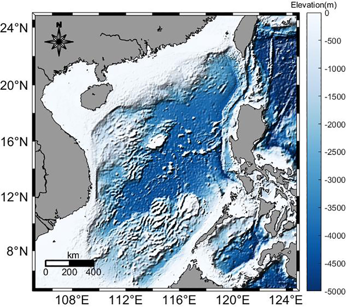
Figure 1 The study area.
2.2. Data
Considering the significance of oceanic predictions in the SCS, the goals of this study involve making extended-range predictions of SSTA and SSHA using convolutional neural networks and transfer learning technology (CNNTL) that are based on remote sensing observations. Moreover, this study also takes the sea surface dynamic processes into account, using the wind speed along with SSTA as input variables to predict SSTA. Both ocean and atmosphere reanalysis data and remote sensing data are used in this study. The reanalysis datasets shown in Table 1, downloaded from Copernicus Marine and Environment Monitoring Service (CMEMS, download from https://resources.marine.copernicus.eu/products) and European Centre for Medium-Range Weather Forecasts (ECMWF, download from https://www.ecmwf.int/en/forecasts/datasets/browse-reanalysis-datasets), are used for the pretraining. These data range from 1 January 1993 to 31 December 2018. Due to data availability, the satellite remote sensing data are restricted to a 3 year period, from 1 January 2018 to 31 December 2020, and are divided into a training set (from 2018 to 2019) and a testing set (2020) for the transfer learning model training. The spatial resolution is the same as that of the reanalysis data, which is 0.25°×0.25°. The data were extracted from an area located at 5°N to 24.75°N and 105°E to 124.75°E; thus, the total number of grids was 80×80. These blended satellite products were used to build and test this deep learning model. The SSH satellite observations are mainly built by combining multiple satellite altimeter missions (Jason-3, Sentinel-3A, HY-2A, Saral/AltiKa, Cryosat-2, Jason-2, Jason-1, T/P, ENVISAT, GFO, ERS1/2) processed by the DUACS multimission altimeter data processing system. SST satellite observations are multiproduct ensembles produced by the GHRSST multiproduct ensemble (GMPE) system at the Met Office. In addition, the 6-hourly blended wind speed is from the WindSat radiometer onboard the Coriolis satellite.

Table 1 Description of reanalysis and satellite remote sensing data.
To eliminate the influence of climate variability on model training, the daily SSHA and SSTA values are calculated based on reanalysis data to train the pretraining model by using the daily values minus the average over the 26 years between 1993 and 2018. In addition, the 6-hourly blended wind speed data was used to calculate daily means.
2.3. CNNTL model
Convolutional neural networks have been adopted to conduct studies successfully since LeCun et al. proposed them in 1998 (LeCun et al., 1998). Generally, CNNs mainly contain an input layer, convolution layer, pooling layer, and fully connected layer (FC). Figure 2 shows an example of a CNN. In the image classification field, the input layer represents the pixel matrix of an image as two dimensional or three-dimensional tensors to input the network. The introduction of convolution and pooling layers makes it superior to traditional neural networks. The convolution layer extracts feature from the network model through a convolution operation, which is a weighted evaluation process that involves sliding convolution filters.
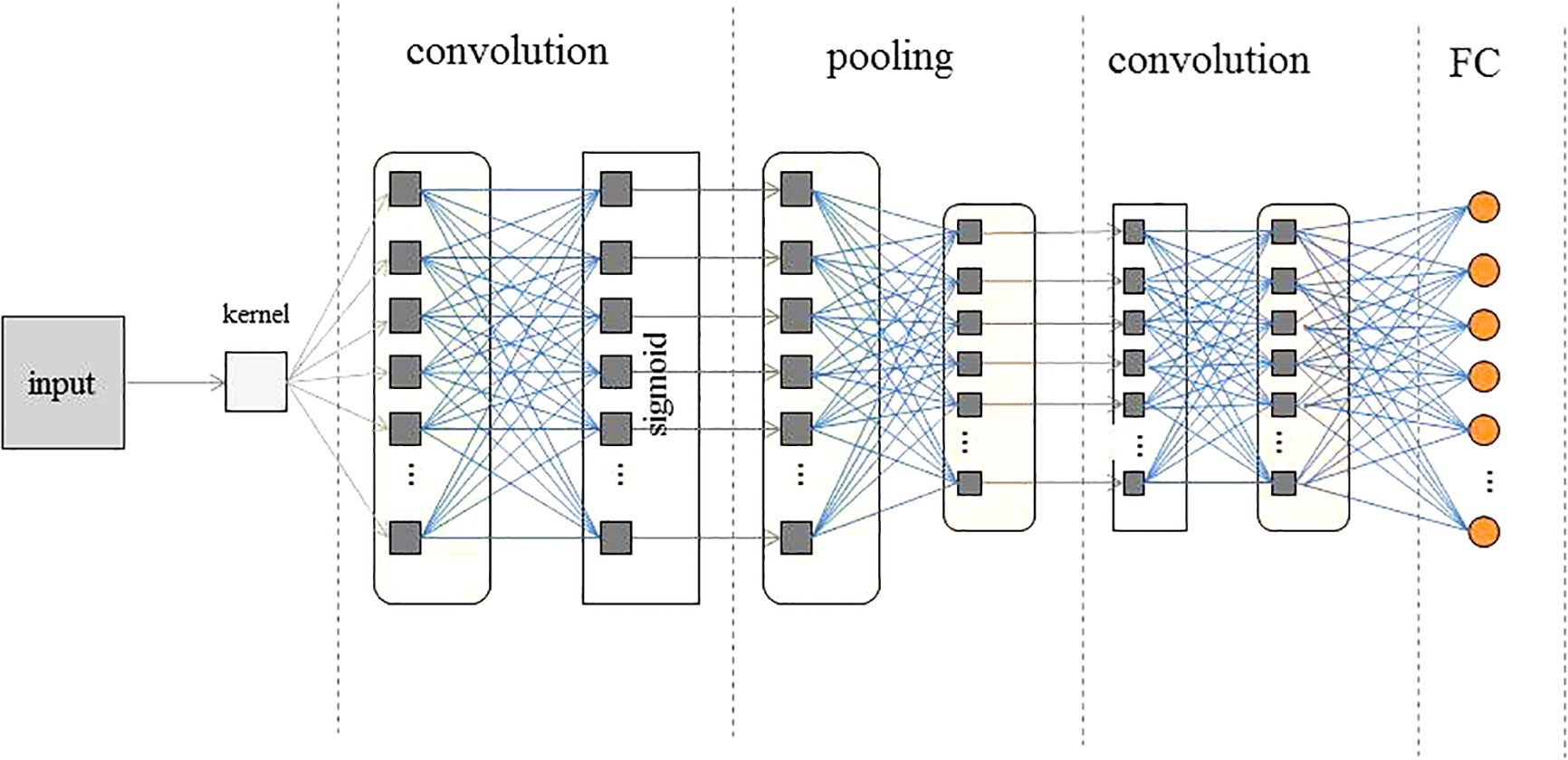
Figure 2 An example structure of a CNN.
As one of the most crucial parts of CNNs, the pooling layer aims to reduce the resolution for further layers and controls overfitting. Mean pooling and max pooling are two main methods. Due to special linear changes in the convolution operation, an activation function layer must be adopted to increase the network nonlinearity before transferring the results to the pooling layer. The common activation functions are sigmoid, ReLU, tanh, Elu, and so on. In addition, a fully connected layer is used to acquire outputs, which integrates the extracted features from the convolution and pooling processes. To accelerate the convergence speed of the gradient descent algorithm and establish a robust model, it is necessary to normalize the training data to a mean of 0 and a variance of 1 with normalization before model training.
In this study, a CNNTL model was constructed for extended-range scale (30 days) predictions of SSHA and SSTA in the SCS. The structure of the CNNTL model is shown in Figure 3. It is mainly composed of 10 convolution layers, 2 pooling layers, 1 fully connected layer and 2 transposed convolution layers. There are 300 convolution kernels for the first two convolution layers with a size of 5×5. The other layers have 30 convolution kernels with sizes of 5×5 (C3 to C5 layer) and 3×3 (C6 to C10 layer). In addition, there is a batch normalization layer after each convolution layer to solve internal covariate shifts in neural network training. This approach was proposed by Ioffe and Szegedy (2015) to improve the generalization ability and training speed of the network. The convolution is a linear process that is difficult to solve linearly inseparable and complex problems in reality. Therefore, to increase the network’s nonlinearity, the activation function, as an effective nonlinear method, is generally used after the convolution layer. The rectified linear unit (ReLU) is a popular activation function that has been widely used in recent studies due to its fast calculation time. The ReLU is defined by selecting the max value between the input data and 0, which leads to the problem of dying neurons, the formula is as follows: φ(z)=max {0, z}. However, the normalized data in this study may have negative values, which indicates that the ReLU is not suitable for using with the data in this study. To avoid this problem, an exponential linear unit (ELU) was used as the activation function here, which was introduced by Clevert et al, 2016. Generally, pooling layers are added to process feature mapping results obtained through convolution operations. These layers summarize the eigenvalues of a position and adjacent positions as the value of this new position. Therefore, this method can reduce the resolution for further layers and avoid overfitting. This study used maximum pooling as a downsampling method to achieve resolution reduction with a size of 2×2, and hence, the feature map dimension can be reduced by half. In addition, the dropout layers are also used to avoid overfitting, which randomly discards the neurons in the training neural network. In this CNNTL model, they are set behind two max pooling layers and the flattened layer with a probability of 0.5. To acquire the same dimension for the output matrix as the input, transposed convolution, an upsampling method, plays an important role in neural networks. This is set to two layers with 30 kernels, and the kernel sizes are 3×3 and 5×5.

Figure 3 Structure of the CNNTL model. This model is composed of ten convolutional layers, ten BN layers, two max pooling layers, one fully connected layer and two upsampling layers.
The CNNTL consists of two main parts. First, a CNN model was trained by reanalysis data to predict SSTA and SSHA at extended ranges (30 time steps, or days). Second, the transfer learning models were retrained by remote sensing data on the basis of the CNN model. The framework of this proposed method is demonstrated in Figure 4.
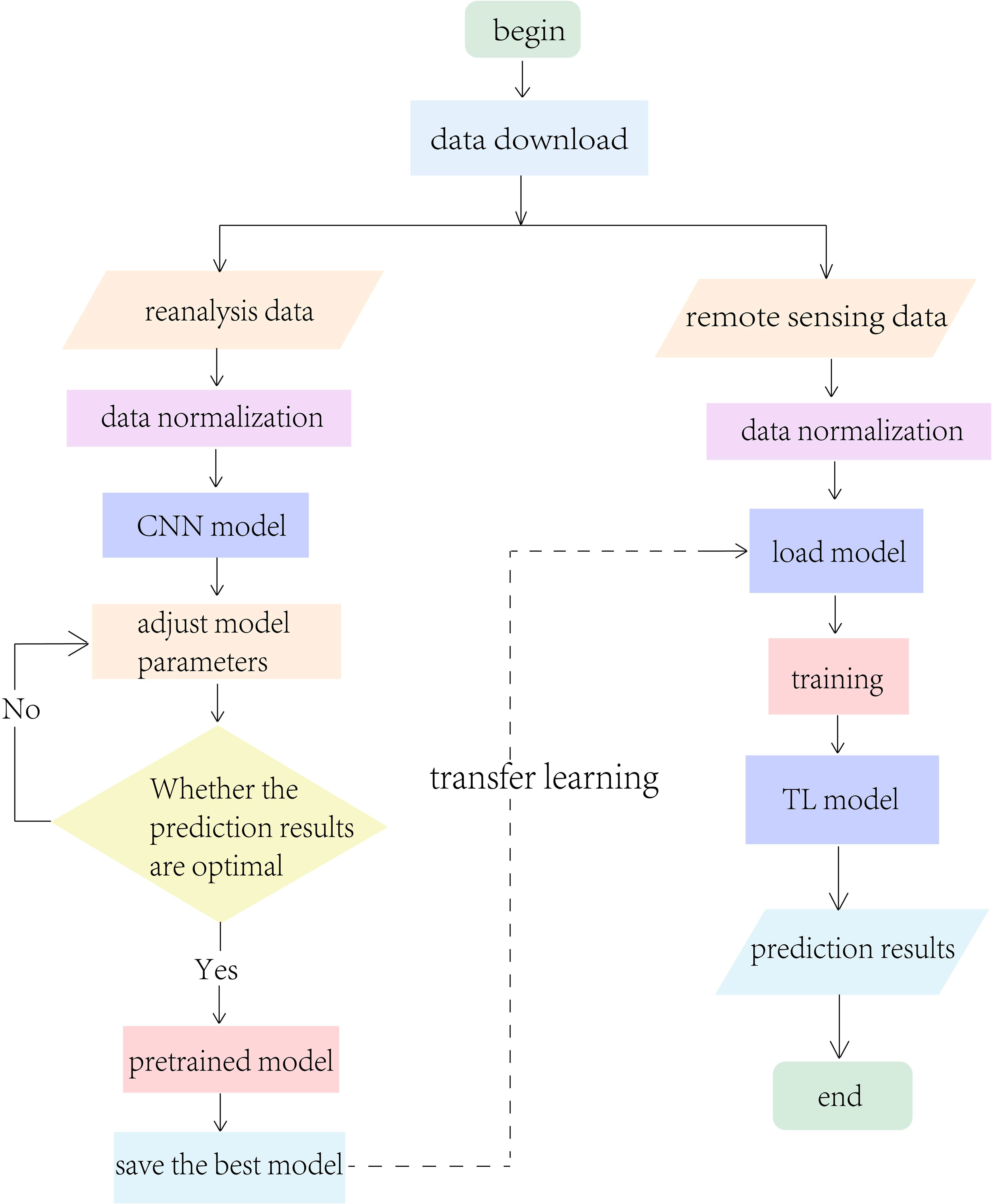
Figure 4 Framework of the proposed prediction model.
The SSTA time series for the previous 14 and current time steps (T-14 to T, i.e., the 1st to 15th steps) along with wind speed data for the future 10 time steps (from T to T+10, i.e., the 1st to 10th steps) were used to predict 30 days of future SSTAs (T+1 to T+30, i.e., the 1st to 30th steps). Notably, the wind speed is the future rather than historical data, and the reasons for this selection are as follows: the wind stress has an obvious correlation with SSTA. It can mix sea water, affect oceanic dynamic processes, and influence latent heat flux by accelerating evaporation, which leads to changes in SSTA. Therefore, the wind speed can play an important role in SSTA prediction. In addition, if this model is adopted for actual applications, the wind speed forecast products (e.g., the ECMWF 10-day wind speed forecast products) can be acquired as input data. In contrast, the SSHA is mainly influenced by quasi-geostrophic currents. Thus, only SSHA was used as an input variable in this study to predict the monthly extended SSHAs. The SSHA time series for the previous 14 and current time steps (i.e., T-14 to T, i.e., the 1st to 15th steps) were used to predict the SSHA of the following 30 time increments. Therefore, the full range of the SSTA (SSHA) time dimension is 25 (15). In this study, “T” indicates the current time. Here, the length of the original reanalysis data sequence was 9490, where the sliding window was set to 1 day. Therefore, 9445 samples were acquired to train the CNN model, and then it was divided into a training dataset and validation dataset, 70% and 30%, respectively. The length of the remote sensing training data sequence was 730 from 2018 to 2019. The data from 2020 were selected as the test dataset. The original remote sensing data were also processed as reanalysis data.
Parameter selection is important for neural networks, such as the loss function and optimizer. The loss function used in this study is the mean squared error (MSE), which intuitively reflects the model’s training quality according to the difference between the training and validation phases. The smaller value of the loss function is, the smaller the deviation between the results obtained by the model and the real value is, that is, the model is more accurate. The optimizer is used to adjust the parameters to reduce the value of the loss function. The Adam optimizer, a deep neural network method for the adaptive learning rate, is used in this study. It dynamically adjusts the learning rate of each parameter using first- and second-order moment estimators of the gradient. Furthermore, the batch size and epoch size are also crucial parameters to reflect the speed of the model convergence and fitting degree, which are set to 128 and 10, respectively.
2.4. Prediction performance evaluation
In this study, the correlation coefficient (CC) and root mean squared error (RMSE) are metrics used to evaluate the performance of the CNNTL model. The CC reflects the degree of linear correlation between variables. As a common measure of the difference between values, the value of the RMSE is usually the metric used to reflect model performance. The smaller RMSE is, the smaller the prediction difference is, and the better the performance of the model is. Specifically, the two metrics are defined as follows:
where N denotes the number of samples and X and Y denote the true matrix and prediction matrix, respectively. Meanwhile, the temporal trends of CC and RMSE are calculated sample by sample at spatial grids during the forecast lead time (30 days).
3. Results and discussions
3.1. Accuracy during the test period
This study constructed a CNNTL model based on transfer learning using satellite remote sensing data to predict the monthly scale extended SSTA and SSHA in the SCS. To better express the degree of accuracy for the extended range scale predictions from the model, a time series of regionally averaged CCs and RMSEs were calculated among the test samples and presented in Figure 5 and Table 2. In general, the CCs and RMSEs of SSTA (SSHA) are stable, fluctuating between 0.6 to 0.79 (0.8 to 0.89) and 0.22°C to 0.32°C (0.020 m to 0.027 m), respectively. Figure 5 shows that the CCs (RMSEs) of the dataset gradually decrease (increase) with an increase in time. When the lead time is 30 days, the CC of SSTA (SSHA) exceeds 0.5 (0.7), indicating that the extended monthly predictions of the CNNTL model is ideal.
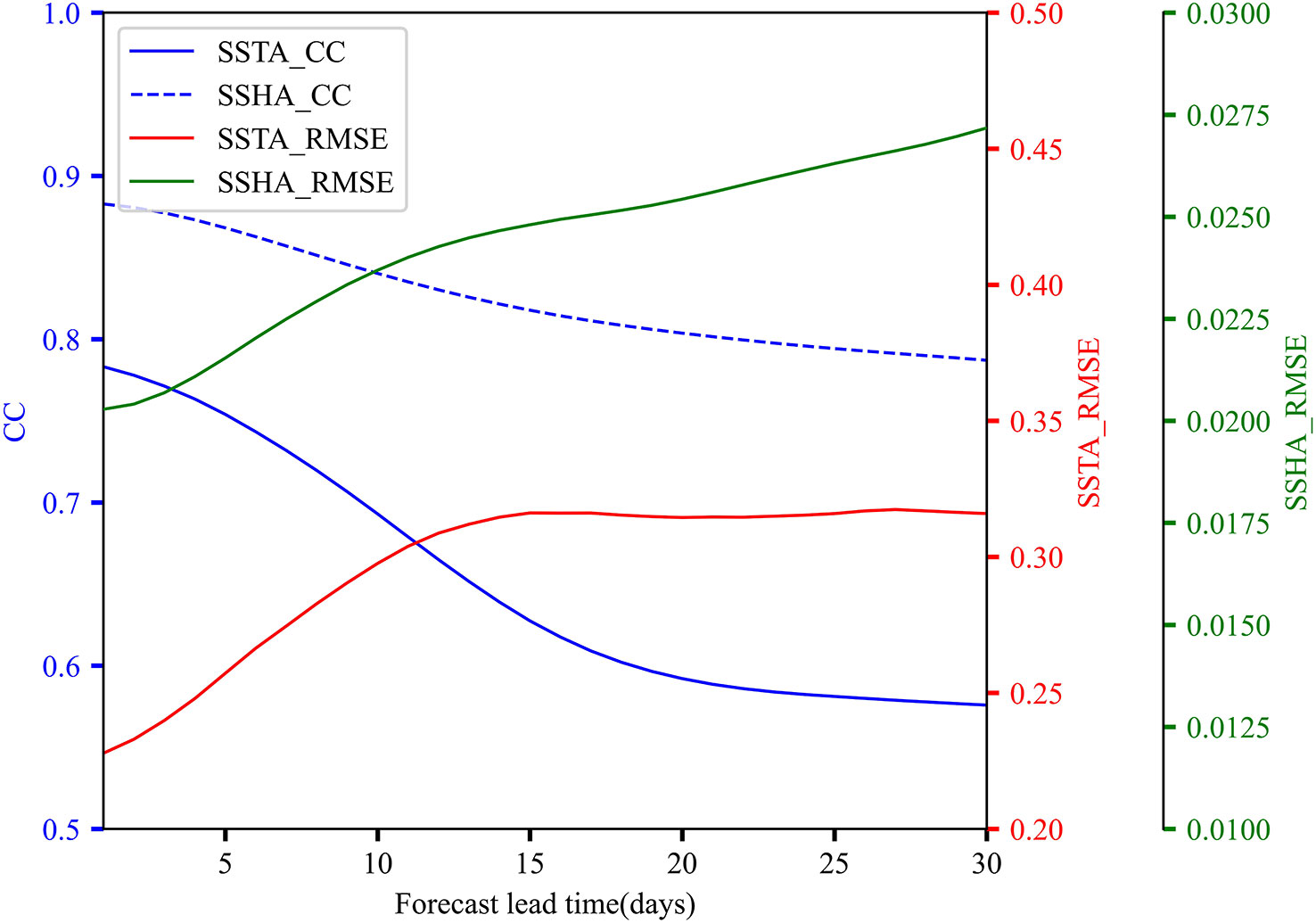
Figure 5 Accuracy of the CNNTL model during the forecast lead time (30 days). Temporal trend of CC (blue solid line: SSTA, blue dotted line: SSHA) and RMSE (red solid line: SSTA, unit: °C; green solid line: SSHA, unit: m).

Table 2 The experimental results of 10-, 20-, and 30-day forecasts.
Furthermore, the spatial distributions of average CC and RMSE of the CNNTL model are given in Figure 6. The average CCs and RMSEs of the prediction made from the 2020 test dataset were calculated grid by grid from daily data over an extended range scale (30 days). As shown in Figure 6A, the CCs of the SSTAs are mainly above 0.6 over most areas of the SCS, showing the availability of the CNNTL model in extended-range prediction. As the predictions progressed, the CCs decreased significantly, indicating that the predictions became less stable as time increased. The overall RMSEs of the SSTAs (Figure 6C) during the prediction are mostly between 0.2-0.5°C, except in the coastal sea region and the south-central SCS. The RMSE in the central sea basin increases distinctly with increasing number of forecast lead days. For the SSHA, CCs are mainly above 0.8 (Figure 6B), and RMSEs (Figure 6D) are mainly 0.01-0.04 m during the prediction. Unlike the SSTAs, the CCs of the SSHA showed greater stability as prediction time increases, indicating the strong prediction ability of SSHA in the SCS. The areas in the northeast along with the north to the west of the SCS have larger RMSEs than the others, which is because these areas have complicated dynamic processes that influence the variation SSHA, more details of which are discussed in section 3.4.
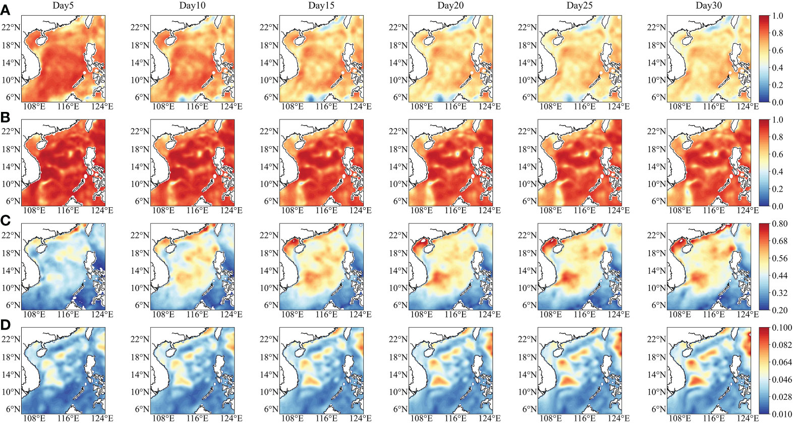
Figure 6 Spatial distribution maps of CC and RMSE on 5, 10, 15, 20, 25, and 30 days. (A) SSTA CC, (B) SSHA CC, (C) SSTA RMSE, unit: °C, (D) SSHA RMSE, unit: m.
3.2. SSTA and SSHA spatial-temporal evolution patterns
Figure 7 shows an example (from 14 June to 13 July 2020) of SSTA spatial maps of satellite observations, predictions, and differences at different prediction times with an interval of 5 days. A strong similarity between satellite observations and predictions can be seen in this figure, which indicates that the CNNTL model has good prediction ability. However, the spatial characteristics between them are slightly different. From Figure 7A, there is mainly a positive anomaly in most areas of the SCS, while the coastal marine area presents a negative anomaly. The SSTA prediction results shown in Figure 7B are consistent with the observations in the most areas of SCS. However, the location and intensity of the negative and positive anomalies have large disagreements with the observations during the prediction lead days, especially along the northern coast. Moreover, from Figure 7A, it can be seen that there was a distinct high value center in the southeast Vietnam, especially when the lead time is 25-days and 30-days. However, it is not obvious in the prediction maps (Figure 7B). The reason may be that this area is the appearance of Vietnam cold eddy which was largely depended by the wind speed. If the wind stress is weaker, the cold eddy may not significant, which makes SSTA higher than the normal. Though the CNNTL model was embedded in wind speed, it only contained future 10 days, which played a minor role in extended-scale prediction. In addition, the spatial distributions differences between prediction and observation are shown in Figure 7C. The differences have no obvious changes during prediction time. The higher values are mainly focus on the Beibu Gulf, southeast Vietnam where the complex dynamic processes occur frequently. The prediction results are overestimated in the northern SCS. However, they are underestimated in most areas of the SCS.
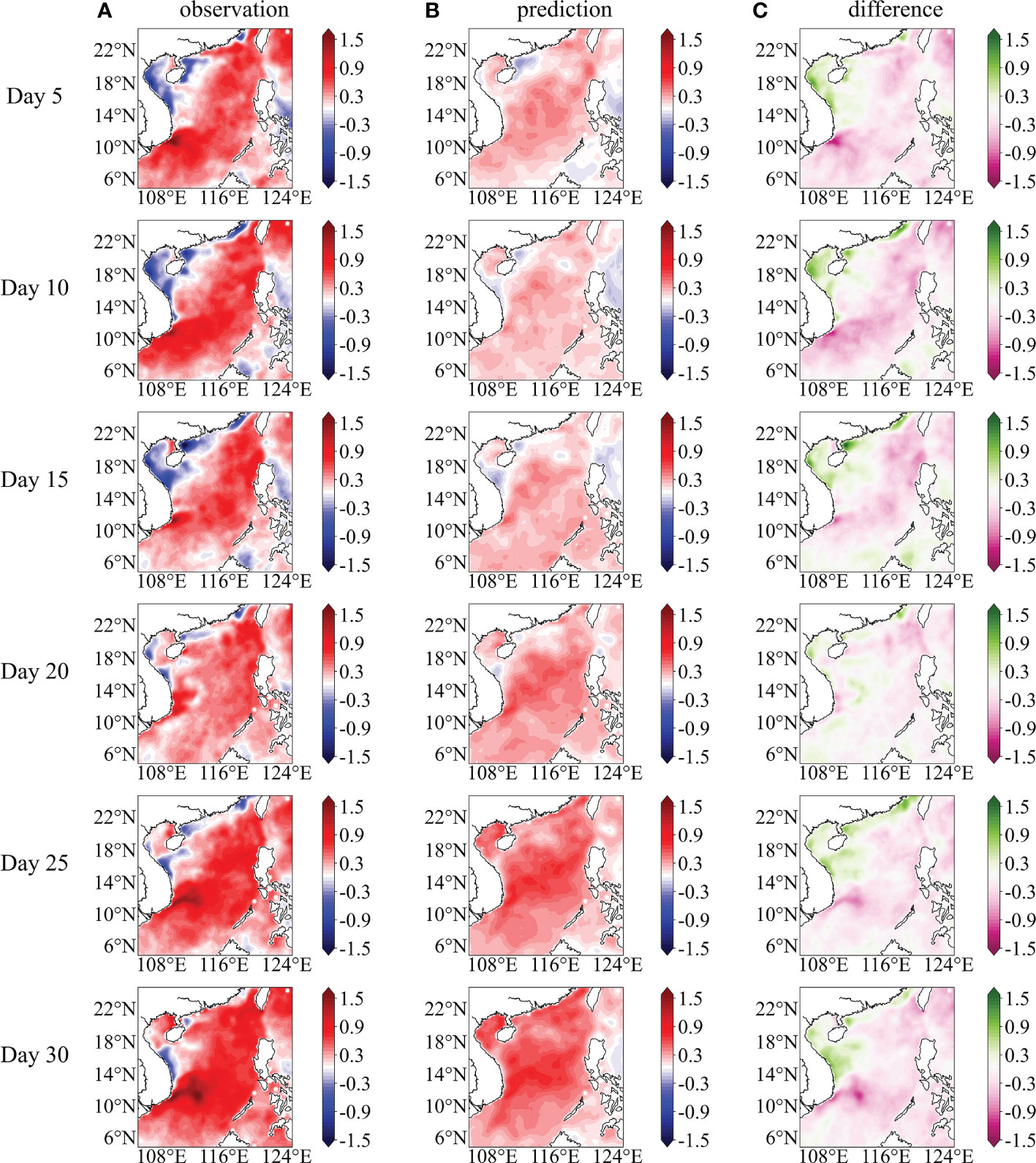
Figure 7 Observation (A), prediction (B), and difference (C) snapshots of sea surface temperature anomaly (SSTA, °C) prediction for 1–30 days (interval of 5 days), corresponding to June 14 to July 13, 2020.
Compared to SSTA prediction, the CNNTL model can capture the spatial-temporal distribution of SSHA more accurately (shown in Figure 8). Figure 8A shows that there was an obvious dipole double eddy structure in the eastern of Vietnam during the period from June 14 to July 13, 2020. In addition, there were obvious warm eddies in the eastern part of Taiwan Island (labeled eddy “a” in Figure 8A-Day 5, the same below) and the eastern part of Luzon Strait (eddy “b”), and cold eddies in the Luzon Strait (eddy “c”), southeastern part of Vietnam (eddy “d”) and western part of Luzon Island (eddy “e” and “f”). Figure 8B shows the prediction results of CNNTL model, it can be seen that there was a strong similarity between satellite observations and the CNNTL predictions in terms of the overall pattern and the characterization of eddies. Specifically, the warm eddies in the eastern Luzon Strait (eddy “a” and “b”), the southwest of Taiwan Island (eddy “g”), the eastern and southeastern Indo-China Peninsula (eddy “h” and “i”) were well captured during the prediction interval. Although the predicted intensity was relatively weaker compared with the satellite observations, the trend of gradual attenuation of two warm eddies in eastern and southeastern Vietnam (eddy “h” and “i”) during the period of June 14 to July 13 was well captured. The cold eddy in southeast Vietnam (eddy “d”) developed gradually during this period. However, this temporal evolution trend was not captured by CNNTL. The model can sufficiently capture the locations of the cold eddies in eastern and western Luzon Strait (eddy “c” and “j”) and the eastern Indo-China Peninsula (eddy “k”), but the prediction intensity is weaker than the actual observations. As the prediction time increases, the spatio-temporal prediction patterns of the CNNTL model can also consistent with the observations, which demonstrates the high performance offered by the model for extended range scale predictions. Figure 8C shows spatial differences of SSHA, it can be seen that the difference displayed nonuniform patterns. The difference values are higher in the locations of mesoscale eddies. According to Figures 8A, B, the areas of warm eddies (the northern and central regions of the SCS) are underestimated, while the areas of cold eddies are overestimated. This pattern remains almost unchanged as the predication time increases, which was consisted with the patterns of the warm eddies and cold eddies. The main reason for this may be that SSHA is mainly affected by the quasi-geostrophic current, showing significant seasonal and interannual variation characteristics and changes slowly over the extended-range scale.

Figure 8 Observation (A), prediction (B), and difference (C) snapshots of sea surface height anomaly (SSHA, m) prediction for 1–30 days (interval of 5 days), corresponding to June 14 to July 13, 2020.
Figures 9 and 10 shows the evolutionary characters of satellite observation and prediction SSHA during prediction lead time (from June 14 to July 13, 2020) at the 21.5°N section and 118°E section, respectively. From the Figure 9, it showed that there was a cold eddy in the eastern of the Luzon Strait, and this pattern can be well captured by the CNNTL model. With the prediction lead time increasing, this cold eddy gradually attenuated firstly, then became stronger and presented a trend of westward motion. Fortunately, the westward motion trend of the CNNTL model prediction was in good agreement with those satellite observations. However, the prediction strength was much weaker than the actual observation. The reason for this may be that influenced by Kuroshio extension and complex topography prominently, the dynamic processes of this area are extremely complicated, which makes the CNNTL model predict difficultly. From the evolutionary maps at the 118°E section shown in Figure 10, the overall patterns of prediction was consistent with observation well within the 10 days prediction windows. But this pattern was not last longer, the prediction strength was much weaker than observation after 10 days. Specially, the cold eddy at approximately 16°N presented a trend of northward motion. The CNNTL model cannot capture this trend too well. The reason may be that Kuroshio intrudes onto the SCS in summer through Luzon Strait in large scale, contributing to the Luzon Strait cold eddy moved northward. And the strength of Kuroshio intruding is influenced by many factors, making the dynamic processes of this area more complex, which makes it more difficult for the model to predict.
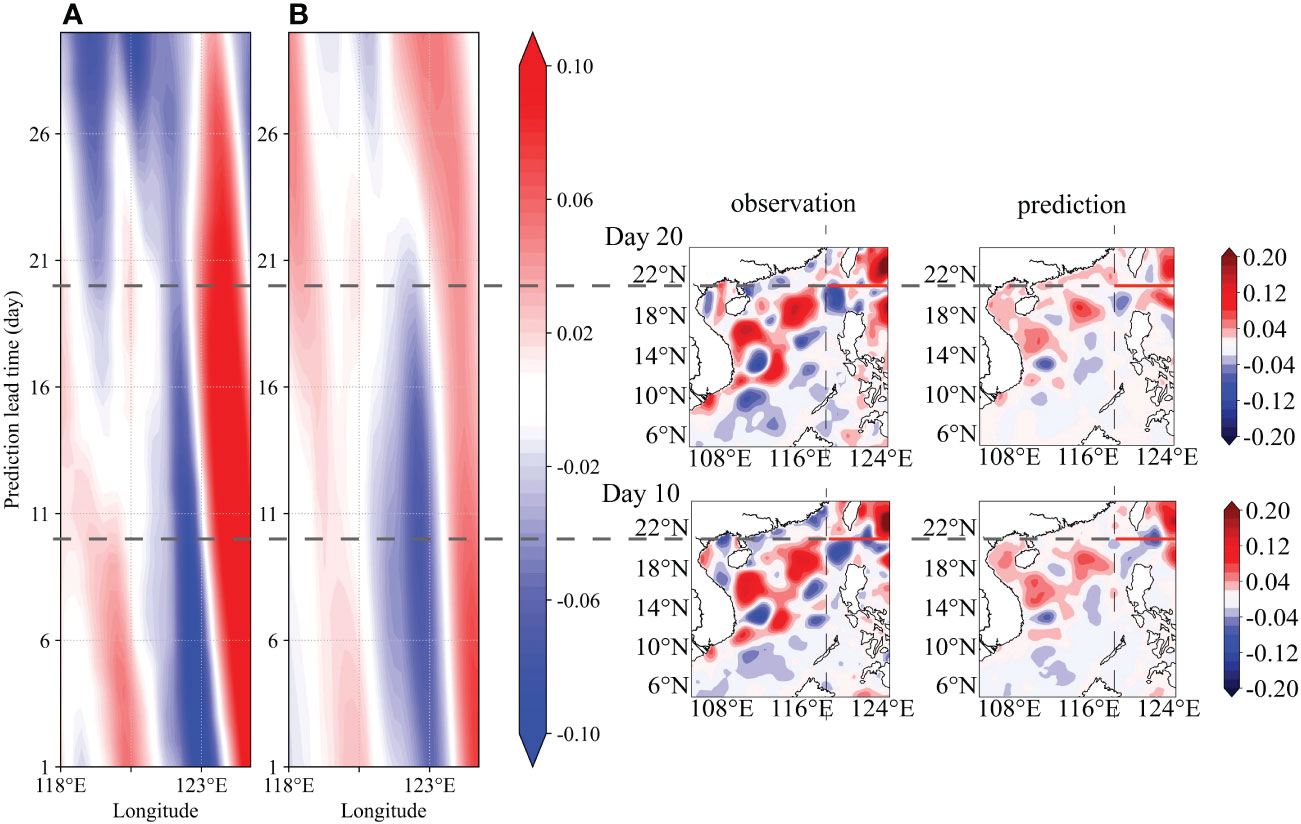
Figure 9 Longitude-time maps at the 21.5°N section. (A) observation, (B) prediction. The red solid line is the longitude range (118°E-124.75°E) of the section.
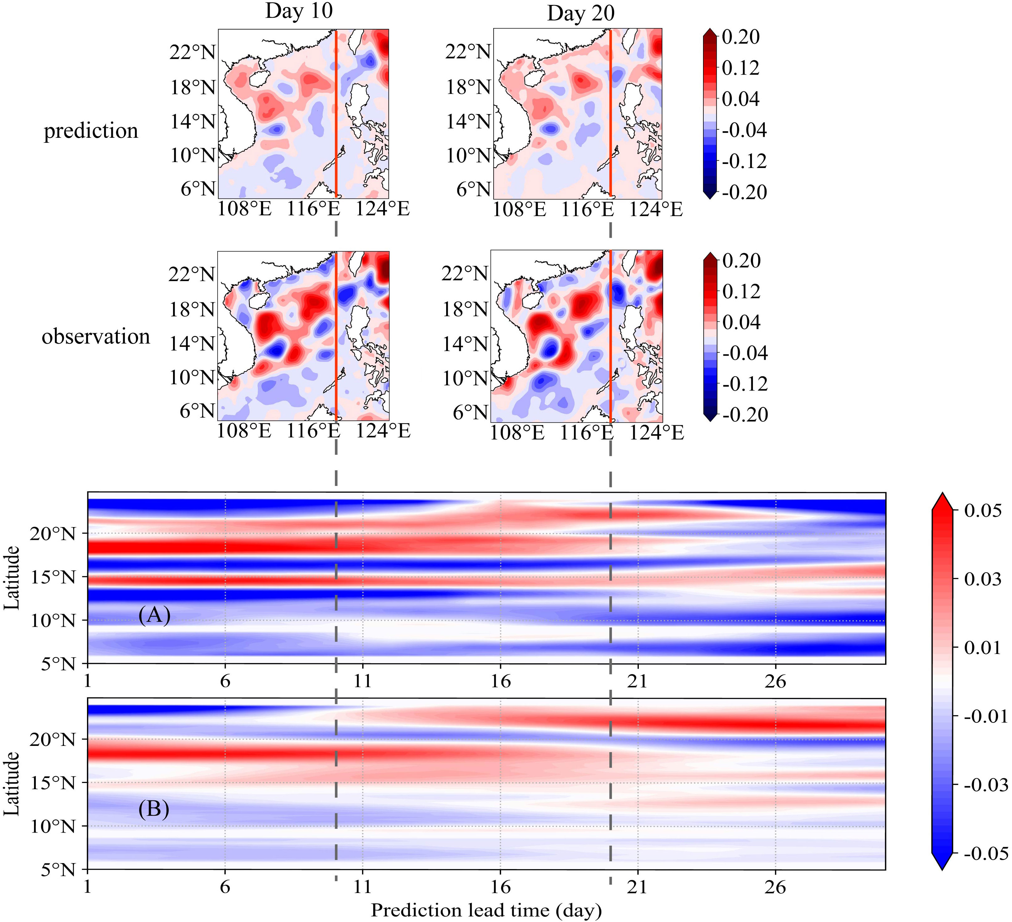
Figure 10 Latitude-time maps at the 118°E section. (A) observation, (B) prediction. The red solid line is the latitude range (5°N-24.75°N) of the section.
Statistical histograms of the SSTA differences and SSHA differences between the predictions and observations over forecast lead days in 2020 are displayed in Figure 11. It can be seen that the statistics of this model have a lower bias and there is a higher proportion of SSTA (SSHA) differences within a range of ±0.5°C ( ± 0.035 m).
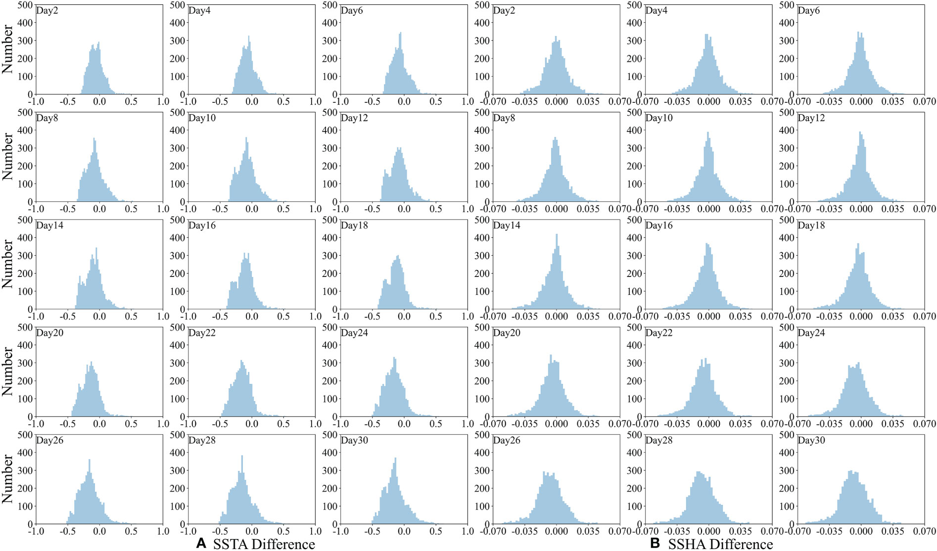
Figure 11 Statistics of the SSTA differences (°C) and SSHA differences (m) between the predictions and the observations in 2020. (A) Shows the SSTA differences (°C) and (B) shows the SSHA differences (m) with leading times from 1 to 30 days.
3.3. Comparison with other models
The comparison of the CNNTL model with the transformer and ConvLSTM model was further quantified. Taking the prediction of SSHA as an example, the RMSEs are shown in Figure 12. It showed that the prediction error of the CNNTL model was stable in the range 0.02-0.03 m within extended-range, with an average RMSE of 0.024 m. Compared with the CNNTL model, the RMSE from the transformer model was less stable and increases significantly with prediction days increasing. It had small error in the initial first day, indicating its suitability for a very short-term prediction. However, it does not preform very well for extended-scale prediction. The average RMSE of transformer model was 0.061 m during the prediction lead time. Besides, the prediction error of ConvLSTM model was more stable than the transformer, but it had higher RMSE during prediction window than the CNNTL model, with the average RMSE of 0.037 m. The RMSEs of tansformer, ConvLSTM, and CNNTL at the end of the prediction window were approximately 0.087 m, 0.041 m, and 0.027 m, respectively. This indicates that the CNNTL model is better than those other two models and has outstanding performance for extended-scale prediction. Notably, both the transformer model and ConvLSTM model used in this study are the basic network models without using other tricks. From the view of the model advancement, both the transformer and ConvLSTM models are more sophisticated than the easy-to-use CNN model, which usually contain the more parameters that need to be fine-tuned to avoid the overfitting and underfitting, thus more data samples are needed to perform the training process for further improving the forecast accuracy.
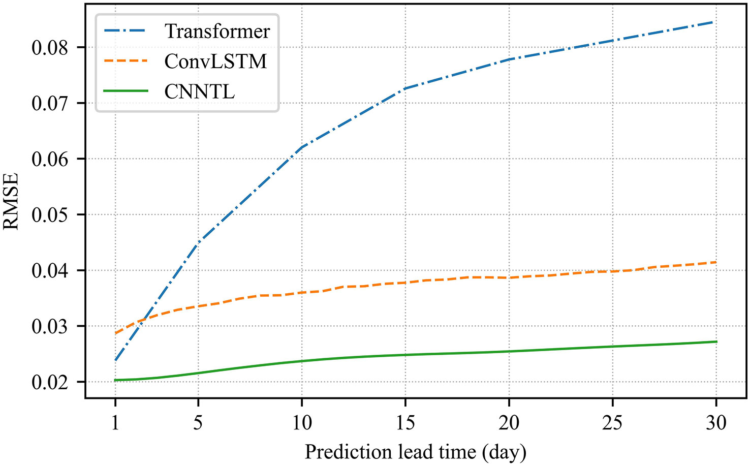
Figure 12 The root mean square error (RMSE, unit: m) of SSHA. The CNNTL model was compared with a transformer model (blue dot dash line), a convolutional long short term memory networks (ConvLSTM) model (orange dashed line), and CNNTL (green solid line).
3.4. Discussion
Based on the above results, when the forecast time is 30 days, the RMSEs of these model predictions for SSTA and SSHA are approximately 0.32°C and 0.027 m, indicating that the CNNTL model performs satisfactorily on an extended range scale. The SCS is one of the most complicated dynamic oceanic areas in the world, having nonlinear and chaotic hydrodynamic processes. From the spatial distribution maps of the RMSEs, the performances of areas are quite different. The RMSEs of the SSTAs and SSHAs are higher in the northern SCS and southeast of Taiwan Island. This is because the area has strong nonlinear dynamical processes, which bring about strong impacts on the CNNTL model prediction and hence lead to a higher RMSE in this area. The predictions are very similar to the satellite observations in terms of the overall pattern and the characteristics, although the changes are not captured well in some areas. From the difference maps of the spatial distribution, the differences in SSTA obviously change in the central sea basin with increasing forecast days. The reasons for these results may be as follows: in principle, the wind stress, which disturbed the sea surface water, can intensify the instability of the SSTAs; in addition, SSTAs are also influenced by other various factors, such as local advection and heat flux, while this CNNTL model only considers wind stress without other factors. Therefore, it limits the performance of this model. The differences in SSHA are higher in the northern part of the central basin. In the SCS, mesoscale eddies are quite active and mainly focus on southwestern Taiwan Island, northwestern and southwestern Luzon Island, and the open sea of Vietnam. They are mainly caused by the following two reasons. First, wind stress forces the upper layer of seawater to move, which can lead to Ekman pumping through divergence and convergence, influencing the eddy kinetic energy (EKE) and then contributing to the strength of mesoscale eddies. Second, the Kuroshio intrusion and baroclinic instability of the background current can change the distributions of SSHAs, which mainly appear in the north of the SCS. Although the accuracy of CNNTL is influenced by those factors, it also offers good results for SSTA and SSHA prediction.
4. Conclusions
Currently, limited by nonlinear chaos predictability, substantial difficulties exist in developing realistic numerical prediction models that operate over longer temporal ranges. However, the rules influencing complicated oceanic processes are hidden within large volumes of spatiotemporal data and can be revealed. Therefore, the growing availability of reanalysis and satellite sensing data makes powerful deep learning technology a promising alternative for predictions and can circumvent certain temporal restrictions. Based on this, a hybrid statistical predication model (CNNTL) for extended predictions of SSTA and SSHA at monthly scales was adopted in this study. This model accurately predicted the spatiotemporal variations in the SSTA and SSHA that are consistent with the satellite observations. For a forecast time of 30 days, the CCs of the model forecasts for SSTA and SSHA were approximately 0.58 and 0.79, respectively. The RMSEs were 0.32°C and 0.027 m, respectively, which are much smaller than those of transformer model and ConvLSTM model. The forecast assuracy of the more robust models are expected to be further improved throuth increasing the data samples and/or using the fine-tune skills. The spatial distribution of the CCs and RMSEs demonstrate that the RMSEs of SSTA are mainly between 0.2-0.5°C during the course of the predication, and the CCs are mainly above 0.6. Except for some sensitive areas that have complex dynamic processes, the CCs and RMSEs of the SSHA are approximately above 0.8 and within 0.05 m, respectively. To further evaluate the model’s performance, this study also analyzed differences in the predication and the satellite observations. For the SSTA results, the positive anomalies were mainly distributed in the northern SCS. For the SSHA, influenced by wind stress, the Kuroshio intrusion and the baroclinic instability of background current, it is obvious that the differences are higher in the central basin, where mesoscale eddies frequently appear. Although influenced by these factors, the CNNTL model demonstrated remarkable performances not only in the temporal trend but also the spatial distribution, indicating that it has sufficient capacity for monthly scale extended predictions. Moreover, the latitude and longitude section results showed that this model can capture the eddy evolutionary accurately. Although the CNNTL model improves the skill of the extended SSTA and SSHA predictions, it can be further improved for applications in the near future. First, the model can be used as a more advanced method to predict monthly scale SSTAs and SSHAs, such as by applying the self-attention mechanism. Second, more factors can be included to more accurately forecast SSTAs and SSHAs and to explore its stability under extreme weather conditions.
Data availability statement
The original contributions presented in the study are included in the article/supplementary material. Further inquiries can be directed to the corresponding authors.
Author contributions
XZ and YM conceived and designed the experiments. YM conducted the data analysis, model validation, writing, and visualization. XZ, YL, DZ, and LZ conducted the formal analysis, review, editing, and supervision. All authors contributed to the article and approved the submitted version.
Funding
This study was funded by the National Key R&D Program of China (2021YFC2803003) and the Open Fund Project of Key Laboratory of Marine Environmental Information Technology, Ministry of Natural Resources of the People’s Republic of China.
Conflict of interest
The authors declare that the research was conducted in the absence of any commercial or financial relationships that could be construed as a potential conflict of interest.
Publisher’s note
All claims expressed in this article are solely those of the authors and do not necessarily represent those of their affiliated organizations, or those of the publisher, the editors and the reviewers. Any product that may be evaluated in this article, or claim that may be made by its manufacturer, is not guaranteed or endorsed by the publisher.
References
Braakmann-Folgmann A., Roscher R., Wenzel S., Uebbing B., Kusche J. (2017). Sea Level anomaly prediction using recurrent neural networks. arXiv. doi: 10.48550/arXiv.1710.07099
Castangia M., Grajales L. M. M., Aliberti A., Rossi C., Macii A., Macii E., et al. (2023). Transformer neural networks for interpretable flood forecasting. Environ. Modell. Software 160, 105581. doi: 10.1016/j.envsoft.2022.105581
Castelluccio M., Poggi G., Sansone C., Verdoliva L. (2015). Land use classification in remote sensing images by convolutional neural networks. arXiv. doi: 10.48550/arXiv.1508.00092
Charney J. G., Fjortoft R., Neumann V. (1950). Numerical integration of the barotropic vorticity equation. Tellus 2, 237–254. doi: 10.3402/tellusa.v2i4.8607
Chen Y., Jiang H., Li C., Jia X., Ghamisi P. (2016). Deep feature extraction and classification of hyperspectral images based on convolutional neural networks. IEEE Trans. Geosci. Remote Sens. 54, 6232–6251. doi: 10.1109/TGRS.2016.2584107
Chen J., Wang X., Xu X. (2022). GC-LSTM: graph convolution embedded LSTM for dynamic network link prediction. Appl. Intell. 52, 7513–7528. doi: 10.1007/s10489-021-02518-9
Clevert D. A., Thomas U., Sepp H. (2016). Fast and accurate deep network learning by exponential linear units (ELUs). arXiv. doi: 10.48550/arXiv.1511.07289
Gorricha J., Lobo V., Costa A. C. (2013). A framework for exploratory analysis of extreme weather events using geostatistical procedures and 3d self-organizing maps. Int. J. Adv. Intelligent Systems 6, 16–26.
Ham Y. G., Kim J. H., Luo J. J. (2019). Deep learning for multi-year ENSO forecasts. Nature 573, 568–572. doi: 10.1038/s41586-019-1559-7
Han M., Feng Y., Zhao X., Sun C., Hong F., Liu C. (2019). A convolutional neural network using surface data to predict subsurface temperatures in the pacific ocean. IEEE Access 7, 172816–172829. doi: 10.1109/ACCESS.2019.2955957
Hervieux G., Alexander M. A., Stock C. A. (2019). More reliable coastal SST forecasts from the north American multimodel ensemble. Clim. Dyn. 53, 7153–7168. doi: 10.1007/s00382-017-3652-7
Hochreiter S., Schmidhuber J. (1997). Long short-term memory. Neural Comput. 9, 1735–1780. doi: 10.1162/neco.1997.9.8.1735
Hu W., Wu R., Liu Y. (2014). Relation of the south China Sea precipitation variability to tropical indo-pacific SST anomalies during spring-to-summer transition. J. Climate 27, 5451–5467. doi: 10.1175/JCLI-D-14-00089.1
Ioffe S., Szegedy C. (2015). Batch normalization: accelerating deep network training by reducing internal covariate shift. arXiv. doi: 10.48550/arXiv.1502.03167
Karpathy A., Toderici G., Shetty S., Leung T., Sukthankar R., Fei-Fei L. (2014). “Large-Scale video classification with convolutional neural networks,” in 2014 IEEE Conference on Computer Vision and Pattern Recognition. 1725–1732. doi: 10.1109/CVPR.2014.223
Kim Y. (2014). Convolutional neural networks for sentence classification. arXiv. doi: 10.48550/arXiv.1408.5882
Kohler M., Langer S. (2020). Statistical theory for image classification using deep convolutional neural networks with cross-entropy loss. arXiv. doi: 10.48550/arXiv.2011.13602
Krizhevsky A., Sutskever I., Hinton G. E. (2012). ImageNet classification with deep convolutional neural networks. Commun. ACM 60, 1097–1105. doi: 10.1145/3065386
LeCun Y., Bottou L., Bengio Y., Haffner P. (1998). Gradient-based learning applied to document recognition. P. IEEE 86, 2278–2324. doi: 10.1109/5.726791
Liu Y., Racah E., Correa J., Collins W. (2016). Application of deep convolutional neural networks for detecting extreme weather in climate datasets. arXiv. doi: 10.48550/arXiv.1605.01156
Long Y., Gong Y., Xiao Z., Liu Q. (2017). Accurate object localization in remote sensing images based on convolutional neural networks. IEEE Trans. Geosci. Remote Sens. 55, 2486–2498. doi: 10.1109/TGRS.2016.2645610
Lorenz E. N. (1963). Deterministic nonperiodic flow. J. Atmos. Sci. 20, 130–141. doi: 10.1175/1520-0469(1963)020<0130:DNF>2.0.CO;2
Luus F. P., Salmon B. P., Van den Bergh F., Maharaj B. T. J. (2015). Multiview deep learning for land-use classification. IEEE Geosci. Remote Sens. Lett. 12, 2448–2452. doi: 10.1109/LGRS.2015.2483680
Masoumi M. (2021). Ocean data classification using unsupervised machine learning: Planning for hybrid wave-wind offshore energy devices. Ocean. Eng. 219, 108387. doi: 10.1016/j.oceaneng.2020.108387
Nageswararao M. M., Zhu Y., Tallapragada V. (2022). Prediction skill of GEFSv12 for southwest summer monsoon rainfall and associated extreme rainfall events on extended range scale over India. Weather Forecast 37, 1135–1156. doi: 10.1175/WAF-D-21-0184.1
Oquab M., Bottou L., Laptev I., Sivic J. (2014). “Learning and transferring mid-level image representations using convolutional neural networks,” in Proc. IEEE Conf. on Computer Vision And Pattern Recognition. 1717–1724. doi: 10.1109/CVPR.2014.222
Pan S. J., Yang Q. (2010). A survey on transfer learning. IEEE T. Knowl. Data En. 22, 1345–1359. doi: 10.1109/TKDE.2009.191
Peng S. Q., Xie L. (2006). Effect of determining initial conditions by four-dimensional variational data assimilation on storm surge forecasting. Ocean Model. 14, 1–18. doi: 10.1016/j.ocemod.2006.03.005
Saha S., Moorthi S., Wu X. (2014). The NCEP climate forecast system version 2. J. Climate 27, 2185–2208. doi: 10.1175/JCLI-D-12-00823.1
Salberg A.-B. (2015). “Detection of seals in remote sensing images using features extracted from deep convolutional neural networks. 2015 IEEE int,” in Geoscience and remote sensing symp (Milan, Italy: IEEE), 1893–1896. doi: 10.1109/IGARSS.2015.7326163
Santana O. J., Hernández-Sosa D., Smith R. N. (2022). Oceanic mesoscale eddy detection and convolutional neural network complexity. Int. J. Appl. Earth Obs 113, 102973. doi: 10.1016/j.jag.2022.102973
Shelhamer E., Long J., Darrell T. (2017). Fully convolutional networks for semantic segmentation. IEEE T. Pattern. Anal. 39, 640–651. doi: 10.1109/TPAMI.2016.2572683
Shi X. J., Chen Z. R., Wang H., Yeung D. Y., Wong W. K., Woo W. (2015). Convolutional LSTM network: A machine learning approach for precipitation nowcasting. arXiv. doi: 10.48550/arXiv.1506.04214
Song T., Han N., Zhu Y. (2021). Application of deep learning technique to the sea surface height prediction in the south China Sea. Acta Oceanol. Sin. 40, 68–76. doi: 10.1007/s13131-021-1735-0
Tong B., Wang X., Fu J. Y., Chan P. W., He Y. C. (2022). Short-term prediction of the intensity and track of tropical cyclone via ConvLSTM model. J. Wind Eng. Ind. Aerod. 226, 105026. doi: 10.1016/j.jweia.2022.105026
Vaswani A., Shazeer N., Parmar N., Uszkoreit J., Jones L., Gomez A. N. (2017). Attention is all you need. arXiv. doi: 10.48550/arXiv.1706.03762
Wang G. H., Li J. X., Wang C. Z., Yan Y. W. (2012). Interactions among the winter monsoon, ocean eddy and ocean thermal front in the south China Sea. J. Geophys. Res. 117, C08002. doi: 10.1029/2012JC008007
Wang Y., Sun H., Wang X., Zhang B., Li C., Xin Y., et al. (2022). MAFormer: A transformer network with multi-scale attention fusion for visual recognition. arXiv. doi: 10.48550/arXiv.2209.01620
Wang G., Wang X., Wu X., Liu K., Qi Y., Sun C., et al. (2022). A hybrid multivariate deep learning network for multistep ahead Sea level anomaly forecasting. J. Atmos. Ocean. Tech. 39, 285–301. doi: 10.1175/JTECH-D-21-0043.1
Zhao J., Guo W., Zhang Z. (2019). A coupled convolutional neural network for small and densely clustered ship detection in SAR images. Sci. China Inf. Sci. 62, 42301. doi: 10.1007/s11432-017-9405-6
Keywords: extended-range forecast, sea surface temperature anomaly, sea surface height anomaly, remote sensing, convolutional neural network, transfer learning
Citation: Miao Y, Zhang X, Li Y, Zhang L and Zhang D (2023) Monthly extended ocean predictions based on a convolutional neural network via the transfer learning method. Front. Mar. Sci. 9:1073377. doi: 10.3389/fmars.2022.1073377
Received: 18 October 2022; Accepted: 28 December 2022;
Published: 16 January 2023.
Edited by:
Shiqiu Peng, State Key Laboratory of Tropical Oceanography, Chinese Academy of Sciences, ChinaReviewed by:
Tao Song, China University of Petroleum, ChinaLin Bo, National Marine Environmental Forecasting Center, China
Guangjun Xu, Guangdong Ocean University, China
Copyright © 2023 Miao, Zhang, Li, Zhang and Zhang. This is an open-access article distributed under the terms of the Creative Commons Attribution License (CC BY). The use, distribution or reproduction in other forums is permitted, provided the original author(s) and the copyright owner(s) are credited and that the original publication in this journal is cited, in accordance with accepted academic practice. No use, distribution or reproduction is permitted which does not comply with these terms.
*Correspondence: Xuefeng Zhang, eHVlZmVuZy56aGFuZ0B0anUuZWR1LmNu; Dianjun Zhang, emhhbmdkaWFuanVuQHRqdS5lZHUuY24=