Time-frequency analysis framework for understanding non-stationary and multi-scale characteristics of sea-level dynamics

Rising sea level caused by global climate change may increase extreme sea level events, flood low-lying coastal areas, change the ecological and hydrological environment of coastal areas, and bring severe challenges to the survival and development of coastal cities. Hong Kong is a typical economically and socially developed coastal area. However, in such an important coastal city, the mechanisms of local sea-level dynamics and their relationship with climate teleconnections are not well explained. In this paper, Hong Kong tide gauge data spanning 68 years was documented to study the historical sea-level dynamics. Through the analysis framework based on Wavelet Transform and Hilbert Huang Transform, non-stationary and multi-scale features in sea-level dynamics in Hong Kong are revealed. The results show that the relative sea level (RSL) in Hong Kong has experienced roughly 2.5 cycles of high-to-low sea-level transition in the past half-century. The periodic amplitude variation of tides is related to Pacific Decadal Oscillation (PDO) and El Niño-Southern Oscillation (ENSO). RSL rise and fall in eastern Hong Kong often occur in La Niña and El Niño years, respectively. The response of RSL to the PDO and ENSO displays a time lag and spatial heterogeneity in Hong Kong. Hong Kong's eastern coastal waters are more strongly affected by the Pacific climate and current systems than the west. This study dissects the non-stationary and multi-scale characteristics of relative sea-level change and helps to better understand the response of RSL to the global climate system.

1. Introduction

Entering the 21st century, global climate change has become a hot issue. It brings us a series of consequences, such as warming temperature, glacier and ice-sheet retreat, global-mean sea-level rise (GMSLR), and the intensification of extreme events (Lelieveld et al., 2016; Roe et al., 2017). Relative sea-level change (RSLC) refers to the change in local mean sea level relative to the local solid surface (Gregory et al., 2019). In the past decades, rising relative sea level (RSL) has resulted in environmental and ecological effects, including the loss of marshes and wetlands, inundation of deltas, erosion of beaches, and the change in salinity (Kirwan and Megonigal, 2013; Passeri et al., 2015). Some typical low-lying coastal regions like Mumbai, Shanghai, Jakarta, Bangkok, London, and New York will be affected (Wang et al., 2012; Strauss et al., 2021). Hong Kong is a developed coastal city with a prosperous economy and high population and infrastructure density. To meet the housing and employment demands, the government has issued the Northern Metropolis Development Strategy, aiming to develop six hundred hectares of land in the northwest New Territories by 2030. However, most of the Northern Metropolis Area is low-lying over the Yuen Long Plain and vulnerable to the rising RSL. Under the SSP3-7.0 scenario, part of Northern Metropolis, Nam Sang Wai, and Mai Po wetlands are projected to be underwater by 2100 (Kulp and Strauss, 2019). Furthermore, rising RSL may inundate the Kwai Tsing Container Terminals, the world’s fourth-largest container port by throughput, and the busy Hong Kong Airport (Strauss et al., 2021). Studying RSLC, including multi-scale periodic changes, long-term trend changes, and non-stationary changes, will provide a scientific basis for Hong Kong’s future regional planning and further understanding of the mechanism of RSLC.

The tide gauges record RSL height relative to the local solid surface, where it is attached, and thus its measurements are influenced by processes that cause sea-surface height to vary as well local vertical land movement (Gregory et al., 2019). The estimated rate of land subsidence in Hong Kong is about -4mm/yr (Ma et al., 2019) and at Quarry Bay station is -4.19 ± 0.26mm/yr (Ding et al., 2001). The long-term trend in RSLC is 3.1 mm/yr when correcting the localized subsidence (Wong et al., 2003). Tide gauge data is important for revealing long-term, cyclical changes in RSL. Non-stationary and multi-scale features are usually detected in RSLC. The temporal non-stationarity of RSLC results from a combination of a long-term trend in the mean RSL, the deterministic tidal component, surge seasonality, and interactions between the tide and surge (Dixon and Tawn, 1999). Many studies also suggest that RSL may have multi-scale oscillatory components from interannual to interdecadal timescales (Karamperidou et al., 2013; Scafetta, 2014; Turki et al., 2020). Hourly to daily extreme RSL related to transient storms, eddies, and tsunamis; seasonal to interannual sea-level dynamics associated with large-scale climate teleconnections and ocean dynamics are considered vital threats to coastal communities, especially, the low-lying areas and sensitive ecosystem areas (Goddard et al., 2015; Lovelock et al., 2017). Therefore, it is necessary to study the non-stationary and multi-scale characteristics of sea-level dynamics.

El Niño–Southern Oscillation (ENSO) and Pacific Decadal Oscillation (PDO) are correlated with global mean sea level (GMSL) (Cazenave et al., 2012; Hamlington et al., 2013). ENSO, a strong interannual climate signal, occurs in the Tropical Pacific. Its variation can not only affect the ecology of the Tropical Pacific, but also the global climate system. El Niño is an unusual warming of surface waters over the central and eastern equatorial Pacific Ocean. La Niña is its cool counterpart (Latif and Keenlyside, 2009). PDO is defined as the leading empirical orthogonal function of North Pacific sea surface temperature (SST) anomalies. The PDO is detected as warm or cool surface waters in the 20°N of the Pacific Ocean (Schneider and Cornuelle, 2005). Such ocean-atmosphere climate variabilities affect RSL along the Pacific by influencing barometric pressure, trade winds, and thermal expansion (Mcphaden et al., 1998; Melet et al., 2018). In our research, we want to explore the response of RSL dynamics in Hong Kong to climate teleconnections.

Studies of interannual to decadal-scale RSLC in Hong Kong have been limited. Ding et al. (2001) analyzed data from two tide gauges over four decades through Wavelet Transform to study the long-term features of Hong Kong RSL. Their result shows that the RSL rose at a rate of 1.9 mm/yr with land subsidence of over 4 mm/yr, and the annual, semiannual, as well as 18.6-year variations are the most significant and stable periodicities according to wavelet analysis. Zhang and Ge (2013) used the multi-fractal temporally weighted detrended fluctuation method to analyze the RSLC in Hong Kong. The research includes three tide gauge stations from 1964 to 2010. Their study identified multi-scale features and long-range correlations of the relative sea-level rise (RSLR) in Hong Kong. However, Zhang and Ge (2013) did not consider the mechanisms of RSLC in Hong Kong and did not explain the physical significance of sea-level multi-fractal characteristics. Previous studies on Hong Kong RSLC have noted the non-stationarity and multi-scale behavior of RSL, but they have not combined these characteristics with the global climate system, and have not used more suitable methods to parse the physical meaning of RSL signals.

In this paper, we analyze tide gauge data from Quarry Bay (QUB), Tsim Bei Tsui (TBT), and Shek Pik (SPW) stations from the 1950s to the 2020s, using the Wavelet Transform to reveal the multi-scale features of RSLC and the Hilbert-Huang Transform to examine the non-stationarity of RSL. We investigate the spatial-temporal heterogeneity of RSLC in Hong Kong and its relationship to ocean-atmosphere climate variabilities such as ENSO and PDO by cross wavelet analysis. This research enhances understanding of the sea-level dynamics on a local scale and the response of RSLC to climate teleconnections.

2. Study area and datasets

2.1. Study area

Hong Kong (22.15°N-22.20°N, 114.07°E-114.14°E) is situated on the southern part of the Pearl River Delta in southern China (Figure 1). To the west, Hong Kong is adjacent to the estuary of the Pearl River and is affected by the fresh water and sediment deposition brought by the Pearl River and Shenzhen River (Zhang and Ge, 2013). The south of Hong Kong faces the vast South China Sea. Hong Kong is bordered to the north by Shenzhen. The northwest of Hong Kong is the low-lying Nam Sang Wai and Mai Po Wetlands where mangroves are abundant. These mangroves provide a habitat for migratory birds in winter and are of great ecological value (Tam et al., 1997). Victoria Harbor is long and narrow, with clusters of buildings on both sides. Victoria Harbor has become narrower in recent years because of land reclamation. Hong Kong also has numerous outlying islands scattered around the near sea.

FIGURE 1

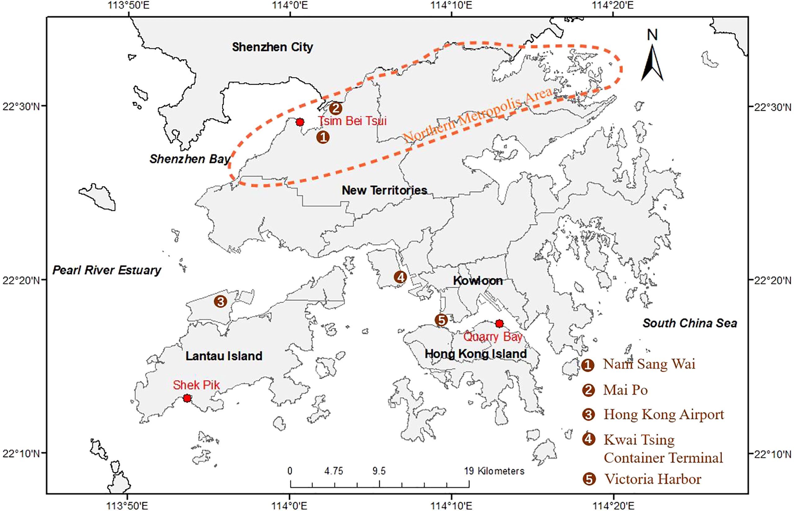
Figure 1 Location of the study area. Red points are the locations of three tide gauge stations.

Hong Kong is significantly influenced by the oceanic subtropical monsoon climate. The weather is mild for nearly the whole year. But between May and November, Hong Kong is subject to tropical cyclones of varying intensity. An average of 30 tropical cyclones form each year over the Pacific Ocean. The approach of tropical cyclones can bring strong winds and heavy rain for days, causing disasters such as landslides, flooding, and extreme sea level. Weather anomalies brought about by global climate change are also likely to affect property and population security in coastal areas.

2.2. Data description and preprocessing

We selected three important tide gauge stations operated by Hong Kong Observatory for analysis (https://www.hko.gov.hk/tc/tide/marine/realtide.htm). They are Quarry Bay (QUB), Tsim Bei Tsui (TBT), and Shek Pik (SPW) tide gauge stations. QUB station has been in operation since 1954. Located within Victoria Harbor, the area is more affected by human activities. The data from this site contain information from both tide and anthropogenic factors like reclamation and land subsidence. TBT station, which began recording in 1974, is situated on the east of the Pearl River estuary and the bottom of Shenzhen Bay, and the west of Mai Po. Northwest Hong Kong is most vulnerable to coastal flooding based on the Climate Central projection. The SPW site, which has worked since 1997, is located on an open shoreline of an outlying island in the south of Hong Kong with fewer anthropogenic factors. Other tide gauge stations were excluded for three possible reasons: short data recording, too much data missing, and difficulty in data acquisition.

Hourly water levels were recorded relative to the Chart Datum, which is 0.146 m below the Hong Kong Principal Datum (Lee et al., 2010). The proportion of valid data for QUB, SPW, and TBT was 98.32%, 93.73%, and 83.05%, respectively. Multivariate Imputation by Chained Equations (MICE) was used to interpolate the missing data through multiple regression models (Royston and White, 2011). It is regarded as an informative and robust method of handling missing data. The daily and monthly data were obtained by calculating the average hourly value.

Indices related to ocean-atmosphere climate variability were also employed in the analysis. National Oceanic and Atmospheric Administration (NOAA) uses the Ocean Nino Index (ONI) for identifying ENSO events. ONI is represented by the running seasonal (3-month) mean SST anomaly for the 5°N-5°S, 120°-170°W (Nino 3.4 region) (Bunge and Clarke, 2009). ONI can be accessed at https://origin.cpc.ncep.noaa.gov/products/analysis_monitoring/ensostuff/ONI_v5.php. PDO index is the leading principal component of an empirical orthogonal function (EOF) of monthly SST in the 20°N–70°N and 110°E–100°W regions (Mantua and Hare, 2002). Similar to the ENSO phenomenon, PDO is characterized by changes in SST, sea level pressure, and wind field. PDO index can be downloaded from: https://www.ncei.noaa.gov/access/monitoring/pdo/.

3. Methods

Fourier Transform and Wavelet Transform are widely used in the analysis of sea-level time series. Fourier transform can provide the frequency components of sea-level signals, that is, the spectra. However, the Fourier Transform is a global transformation in the time domain defined by the sine base functions of an infinite interval and therefore is only applicable to the analysis of global spectra, not to the analysis of local spectra. The Wavelet Transform allows for different selections of base functions. Moreover, the variability and period of the time-series signals can be captured by Wavelet Transform. Thus, is more appropriate than Fourier Transform for analyzing non-stationary signals due to meteorological or geophysical effects (Drago and Boxall, 2002; Grinsted et al., 2004; Sreedevi et al., 2022). Hilbert-Huang Transform (HHT) was born by drawing on the strengths of the multi-resolution of the Wavelet Transform while overcoming the difficulty of selecting the wavelet base functions. HHT is also an effective time-frequency analysis tool for non-stationary signals (Huang, 2014) and is good at analyzing non-linear natural phenomena, like extracting meteorological and oceanic signals (Chen et al., 2017).

The time-frequency analysis framework is developed to incorporate the non-stationarity and multi-scale features of RSLC, by using the Wavelet Transform and HHT method. First, the tide gauge data applied in this research was interpolated using appropriate interpolation methods if a part of the data is missing. Particularly, the MICE algorithm was adopted to reconstruct the missing data. Second, time-frequency analysis was applied to the complete tide gauge data. The Wavelet Transform and HHT methods are effective time-frequency analysis tools. The Wavelet Transform is mainly used to reveal the multi-scale information of RSLC, while the HHT method is more used to capture and amplify the non-stationary details of sea-level dynamics. Finally, both the multi-scale periodic features and non-stationary features were used to investigate the relationship among RSLC, ENSO, and PDO.

3.1. Multi-scale periodic features of RSLC based on the wavelet transform

Tidal amplitude and RSL exhibit multi-scale periodical changes. The driving factors of seasonal, annual, and long-periodic tidal amplitude are complex. Possible factors include the distribution of continents, the influence of monsoons and meteorological events, and GSLR (Idier et al., 2019). Therefore, choosing an appropriate method to analyze the multi-scale characteristics of RSLC is helpful for us to understand the mechanism of RSLC.

The Wavelet Transform is a method for time-frequency analysis. It is important to select the wavelet base function. The appropriate base function can represent the signal with few vectors to the maximum extent, and improve the adaptability of the Wavelet Transform. In this research, the Morlet wavelet was used to reveal the spectral feature and the period of RSLC in Hong Kong (Morlet et al., 1982). The definition of the Wavelet Transform is:

$\begin{array}{ll}{W}_{\psi }^y\left(\text{a},\text{b}\right)=\frac{1}{\sqrt{a}}\underset{-\infty }{\overset{\infty }{\int }}y\left(t\right)\psi \left(\frac{t-b}{a}\right)dt& (1)\end{array}$

where ψ(t) represents the Morlet wavelet, ɑ is called dilatation, and b is the translation parameter. From the formula (1), it can be seen that the spectrum characteristic could be revealed by the time-frequency analysis of time series y (t).

3.2. Non-stationary features of RSLC based on the HHT

The HHT has been widely applied in geographical research to study non-stationary and non-linear signals, like precipitation, solar radiation, and sea level height (Duffy, 2004; El-Askary et al., 2004; Ezer et al., 2013). These studies indicate that the HHT method has advantages in the decomposition of non-stationary signals and the capture of abnormal phenomena, and has great potential for analyzing RSLC. Empirical Mode Decomposition (EMD) and Hilbert Transform are the two main steps of this method. The EMD process decomposes a time series signal y(t) into several intrinsic mode functions (IMFs), which are the components of the original signals. Firstly, all the local extrema in y(t) are identified. Then, the upper and lower envelopes of y are connected separately based on the local maxima and local minima. Through two envelope curves, the mean is computed. This process is repeated iteratively until the stopping condition is satisfied. This process is then applied to the residual time series r₂ = r₁–c₂. Subsequent IMFs c₃…, c_n and residuals r₃…, r_n are obtained similarly. The sifting process terminates when r_n has at most one extremum. The initial time series y(t) has then been decomposed as:

$\begin{array}{ll}y\left(t\right)={\displaystyle {\sum }_{j=1}^n{c}_j\left(t\right)}+r_n\left(t\right)& (2)\end{array}$

In mathematics and signal processing, the Hilbert Transform is the convolution of the signal 1/(πt) and signal f (t) in the time domain (Junsheng et al., 2006). The Hilbert transform $\widehat{f}\left(t\right)$ of a real function f (t) is defined for all t by:

$\begin{array}{ll}\widehat{f}\left(t\right)=\frac{1}{\pi }P\underset{-\infty }{\overset{\infty }{\int }}\frac{f\left(\tau \right)}{t-\tau }d\tau & (3)\end{array}$

3.3. Relationship between RSL and climate teleconnection

3.3.1. Cross wavelet transform

Based on the Wavelet Transform mentioned above, we further applied cross wavelet analysis to study the teleconnections between RSL and global climate systems. Cross wavelet analysis can not only analyze the degree of cross-correlation between signals but also obtain the phase relation of signals in the time-frequency domain. The cross wavelet transform (XWT) of two time sequences x_n and y_n is defined as W^XY = W^XW^Y*, where * represents complex conjugation. The cross wavelet power is defined as |W^XY| . With background power $P_k^X$ and $P_k^Y$, the distribution of the cross wavelet power of two time sequences is defined as (Torrence and Compo, 1998):

$\begin{array}{ll}D(\frac{W_n^X\left(s\right)W_n^{Y*}\left(s\right)}{\sigma X\sigma Y}<p)=\frac{{\text{Z}}_v\left(p\right)}{v}\sqrt{P_k^X{P}_k^Y}& (4)\end{array}$

where Z_v(p) is the confidence level.

3.3.2. Wavelet coherence

Area with high common power can be revealed through cross wavelet power, while how coherent the XWT in the time-frequency domain can be displayed using wavelet coherence (WTC) (Grinsted et al., 2004). The wavelet coherence between two time sequences can be expressed as:

$\begin{array}{ll}{R}_n^2\left(\text{s}\right)=\frac{{\left|\text{S}\left(s^{-1}{W}_n^{XY}\left(\text{s}\right)\right)\right|}^2}{\text{S}\left(s^{-1}{\left|W_n^X\left(\text{s}\right)\right|}^2\right)\text{S}\left(s^{-1}{\left|W_n^Y\left(\text{s}\right)\right|}^2\right)}& (5)\end{array}$

where S is a smoothing operator.

4. Results

4.1. Multi-scale periodicity of RSL

Periodicities of RSLC were studied using the time-frequency spectrum of the Wavelet Transform. Periodic changes in RSL are summarized in Figure 2 and Table 1. In Figure 2, the real part of wavelet coefficients was shown using contour images. Figures 2A–C display the wavelet spectrum at the QUB, TBT, and SPW tide gauge stations, respectively. Red represents periods of high RSL and blue represents periods of low RSL. Based on the wavelet variance (Figures 3A–C), we found that there is a first major period (Figure 3D) at different tide gauges on different time scales. For the QUB station, when the timescale is 500 months, the first major period of RSLC is about 350 months, with about 2.5 cycles of high-to-low sea-level transition. For TBT and SPW sites, time scales for the first major period are 350 and 200 months, and the first major period of RSLC is about 250 and 125 months, respectively. The first major period of RSL at both QUB and TBT is significant with a confidence level above 95%. The specific high RSL and low RSL periods and their corresponding time scales for different tide gauge stations are shown in Table 1.

FIGURE 2

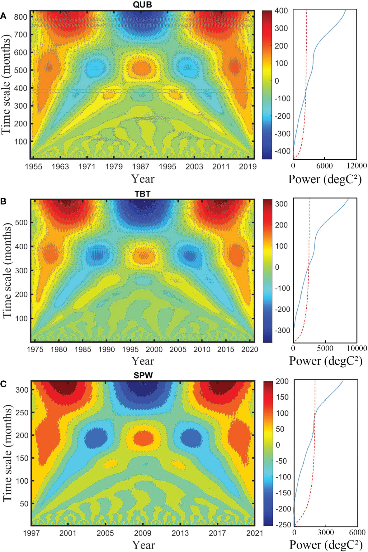
Figure 2 Wavelet transform (left) and global wavelet spectrum (right). (A–C) are wavelet coefficient contour images and global wavelet power the at the QUB, TBT, and SPW tide gauge stations, respectively. The result is significant when the global wavelet spectrum (blue line) is higher than the 95% confidence level (dotted red line).

TABLE 1

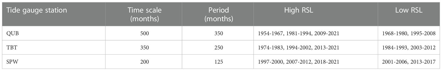
Table 1 First major period and the period scale of three tide gauge stations.

FIGURE 3

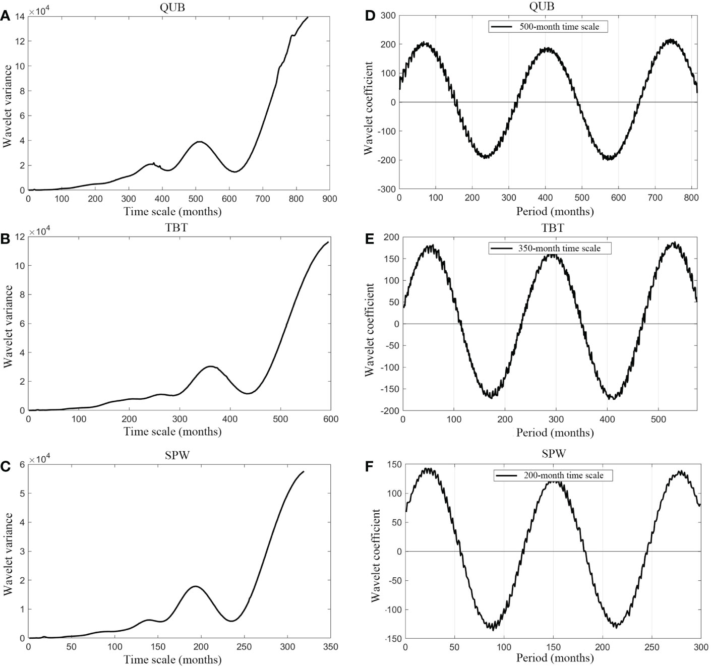
Figure 3 Wavelet variance and wavelet coefficient at different tide gauges. (A–C) are wavelet variances at the QUB, TBT, and SPW tide gauge stations, respectively. (D–F) are the wavelet coefficient of QUB, TBT, and SPW at their first major period, respectively.

The modulus of the wavelet coefficient displays the distribution of energy density in the time domain corresponding to variations on different time scales. A more significant periodicity of the corresponding time scale can be shown by a larger modulus of the wavelet coefficient. According to the modulus of the wavelet coefficient, the periodicity of sea-level variations at the three stations is obvious on the time scale of around 18 to 20 months (Figures 4A–C), which is nearly occupies the whole research time scale. Besides, the periodic change of sea level shows a local pattern. At the TBT station, from 1985 to 1993, the periodic change of sea level is significant when the period is 25-55 months (Figure 4B).

FIGURE 4

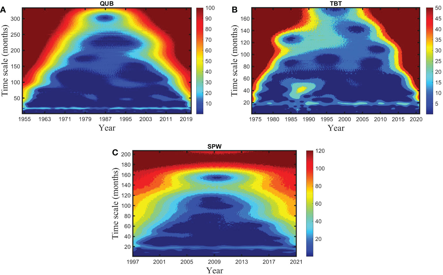
Figure 4 Modulus of the wavelet coefficient. (A–C) are the modulus of the wavelet coefficient at the QUB, TBT, and SPW tide gauge stations, respectively.

4.2. Decomposition of sea-level signals in Hong Kong

Figure 5 shows the IMF components of sea-level signals at the three tide gauges. There are 9 or 10 IMF components in total contained in the original sea-level signals. All the IMF components are above the 95% confidence level in three tide gauges, indicating that these significant components include considerable information with physical meaning. Linear regressions were conducted based on the tide gauge data at three stations. At QUB station, the RSL first experienced a fall with an annual rate of 6.2 mm/yr from January 1954 to October 1972, and then rose at 1.9 mm/yr for nearly 41 years. From May 2013 to November 2021, the RSL showed a slight downward trend at an annual rate of around 0.7 mm/yr (Figure 6A). Similarly, the RSL at SPW also decreased by 9.9 mm/yr from 1997 to 2004, then rose by 1.7 mm/yr between the summer of 2004 and the autumn of 2019. Finally, the RSL fell 10.6 mm/yr by November 30, 2021 (Figure 6C). The RSLC tendency at the TBT station is different from the other two stations. RSL experienced an initial 22-year decline (2.2 mm/yr) and a subsequent 25-year rise (3.6 mm/yr) (Figure 6B). EMD and linear regression results show that although the RSL is rising in the overall trend, there is also a relative decline in different stages. Shortly, the RSL near Victoria Harbor and Lantau Island may continue to decline, but the RSL in the Pearl River Delta may continue to rise.

FIGURE 5

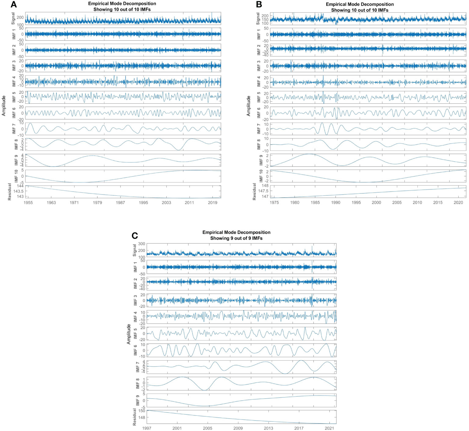
Figure 5 EMD results of three tide gauge stations. (A–C) show the original daily sea-level signal (units: cm), a series of IMF components, and residual of QUB, TBT, and SPW tide gauge sites, respectively.

FIGURE 6

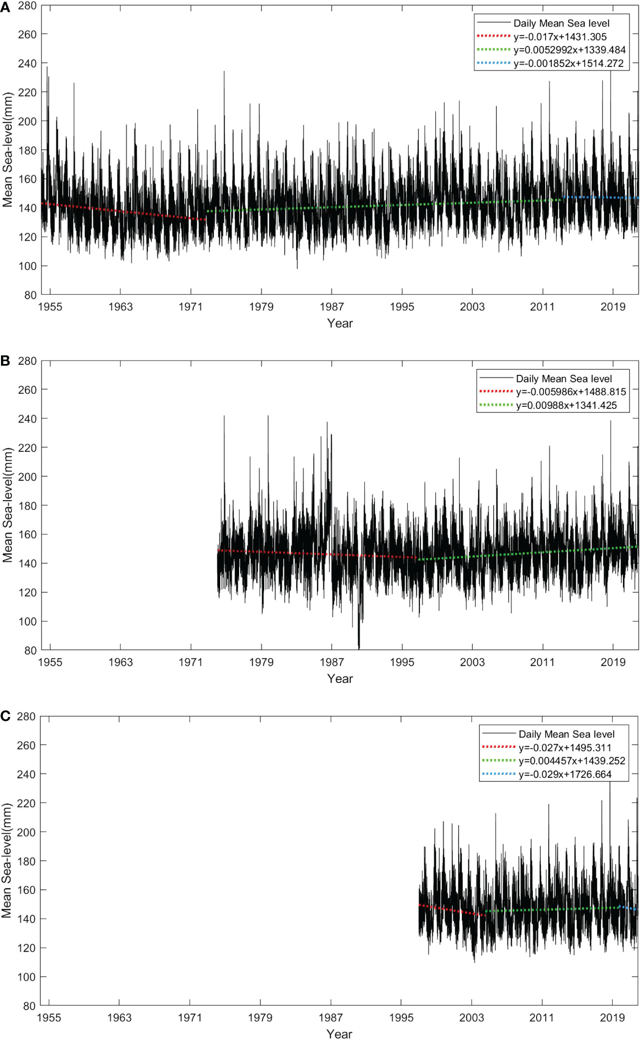
Figure 6 Daily tide gauge data. Linear regression of daily mean RSL based on the last IMF component of EMD results. (A–C) are the QUB, TBT, and SPW, respectively.

4.3. Non-stationarity of RSLC

We applied HHT to tide gauge signals. The Hilbert spectrum shows the three-dimensional information of time series in terms of time, frequency, and energy. In Figure 7, the x-axis represents the years. The y-axis represents the period. The tidal amplitude is presented with the red-green-blue color scheme, where red represents large tidal amplitude, and blue represents small tidal amplitude. At the QUB station (Figure 7A), when the period is about 100 days or 3 months, the years with large tidal amplitudes are 1955 (moderate La Niña), 1974 (weak La Niña), 1977 (weak El Niño), 2002 (moderate El Niño), and 2017 (weak La Niña). With a 40-50 days period, the large amplitude years are 1963, 1964, 1969, 1972, 1994, 2004, 2007, and 2012 (Figure 7A). Similarly, these years have been recorded with ENSO events. At TBT station, the most significant periods are in 1987 and 1990 with periods of about 150 days. They correspond to a strong El Niño and less precipitation, respectively. The major years with large sea-level amplitudes and 40-50 days periods are 1998, 2003, 2006, 2010, 2015, and 2017. These years also clearly correspond to the ENSO phenomenon except for 2003 (Figure 7B). Hilbert spectrum reflected very little rainfall during 2003 (12% rainfall less than normal). The Hilbert spectrum of the SPW station (Figure 7C) also marks down some years with large amplitude anomalies. The years with large tidal amplitudes are 1998, 2003, 2017, and 2020. Their period is around 30 days. The other three years corresponded to the ENSO phenomenon, but the large tidal amplitude in 2003 was due to very little precipitation. At the same time, 2015 saw a very strong El Niño with a period of about 20 days.

FIGURE 7

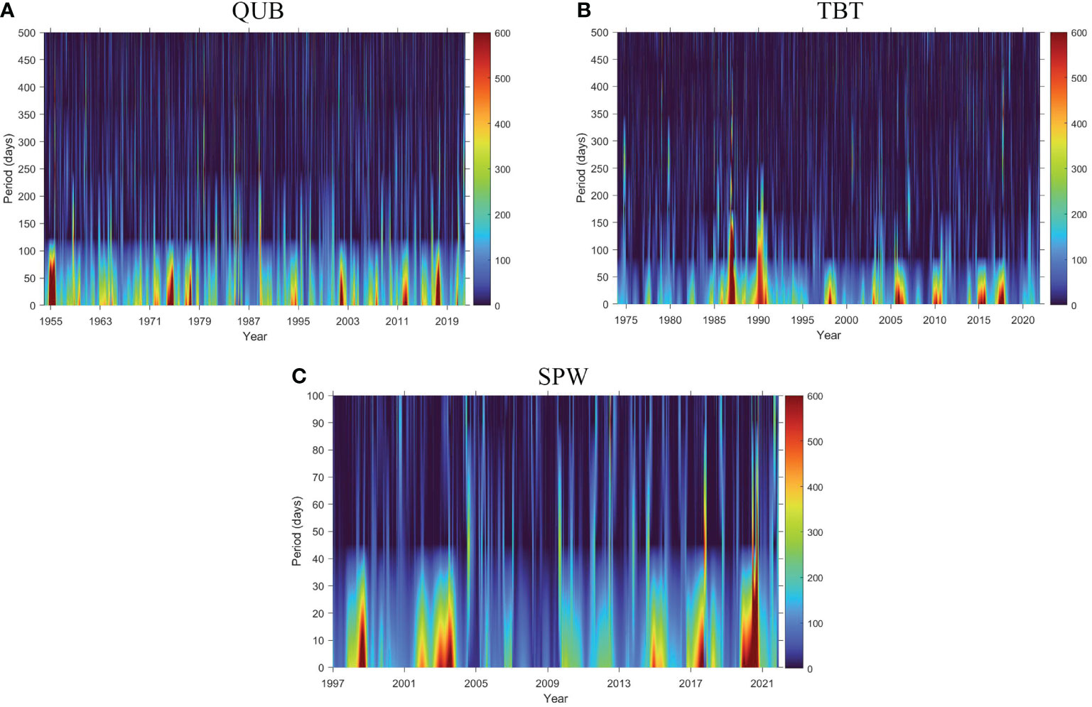
Figure 7 The Hilbert spectrum of three tide gauge stations. X axis represents the years. Y axis represents period. Color bar present the intensity of tidal amplitude. Red represents large tidal amplitude, while blue represents small tidal amplitude. (A–C) are the QUB, TBT, and SPW tide gauge stations, respectively.

When ONI is between -0.5 and 0.5, it means there are no ENSO events in the year. ONI values of 0.5 to 1.1 to 1.5, and 1.5 to 2 correspond to weak, moderate, and strong El Niño events, respectively (Figure 8). ONI greater than 2 indicates a very strong El Niño year. Similarly, the ONI value ranging from -0.5 to -1, -1 to -1.5, and -1.5 to -2 corresponds to weak, moderate, and strong La Niña years. When comparing the ONI and the Hilbert spectrum of three tide gauge stations, the results show that the HHT captured most years of ENSO events. In addition, years of significant events such as heavy annual rainfall or drought were reflected by the HHT. The periodic changes and non-stationarity in sea-level fluctuations are revealed during the HHT analysis.

FIGURE 8

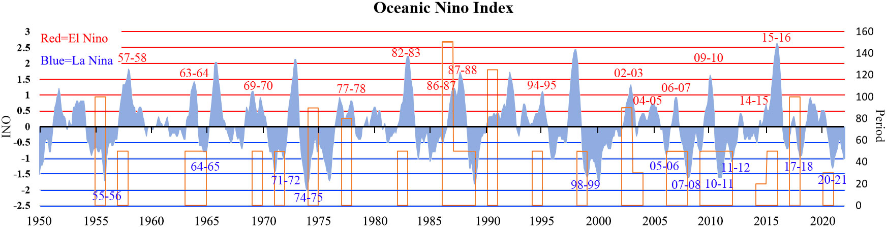
Figure 8 ONI of each year since 1950. The ENSO events captured by HHT were marked over the years. Red numbers represent El Niño years recorded by the Hilbert spectrum, and blue numbers represent La Niña years recorded by the Hilbert spectrum. The intensity of ENSO events could be checked in the left part. The orange bars represent the ENSO years recorded by the Hilbert spectrum, the period of which can be seen on the right part.

4.4. Relationship between RSL and ENSO and PDO

To better analyze the relationship, detailed features, and variation rule between ocean-atmospheric climate variability and RSL in three tide gauge stations in the time-frequency domain, spectrum maps are drawn by using XWT and WTC. The statistical significance against red noise backgrounds can be assessed through Monte Carlo methods (Metropolis and Ulam, 1949). The XWT finds the region of the time sequences with the same high power and periodic intensity in the time-frequency domain. While WTC finds regions in the time-frequency domain where two time sequences co-vary together, but not necessarily with high power. The continuous wavelet power spectrum was shown adopting the red-green-blue color scales. The color shows the intensity of periodicity. Red represents strong periodicity, Blue represents weak periodicity. The region of the thick solid contour represents the standard spectrum of red noise tested at the significance level α=0.05. The thin arc region represents the effective spectral value of the cone of influence (COI), where a lighter shade shows the image that might distort by edge effects. The arrow indicates the relative phase relationship. The arrows pointing right mean the RSL and ocean-atmosphere variabilities are in-phase.

Figures 9A, B shows the WTC spectra of ocean-atmosphere variabilities and the RSL at the QUB site. During 1957-1973 and 1976-1985, ONI and the RSL showed strong coherence, with a coherence coefficient of more than 0.9, which passed the 95% confidence test. Moreover, most arrows face to the left and the two signals are in anti-phase, indicating that the change of ONI leading RSL 1/2 period, that is, 10-16 months (Figure 9A). Figure 9B, during 1960-1969, and 1982-2000, PDO and the RSL are highly coherent and in anti-phase. PDO led the RSL around 16 months and 30 months in 1960-1969, and 1982-2000, respectively. However, PDO lagged RSL for around 24-48 months during 1971-1982.

FIGURE 9

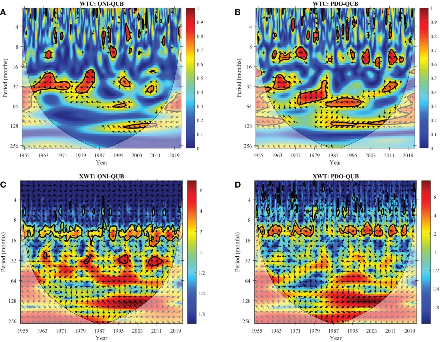
Figure 9 WTC and XWT spectrum of ocean-atmosphere variabilities and the RSL at QUB site. (A, B) are the WTC spectrums of ONI-QUB and PDO-QUB. (C, D) are the XWT spectrums of ONI-QUB and PDO-QUB.

Figures 10A, B displays the WTC results of ONI, PDO, and RSL at the TBT station. Figure 10A indicates that ONI and the RSL are highly correlated when the period is around 30 months, during 1988-1991. ONI leading RSL approximately 12 months. In Figure 10B, When the period is about 10-15 months, PDO and RSL show strong coherence in 1992, 1995, 2002, 2007, 2013, and 2017. Most of the arrows are to the left, indicating the PDO is 1/2 or 3/8 periods (about 5 months) ahead of RSL.

FIGURE 10

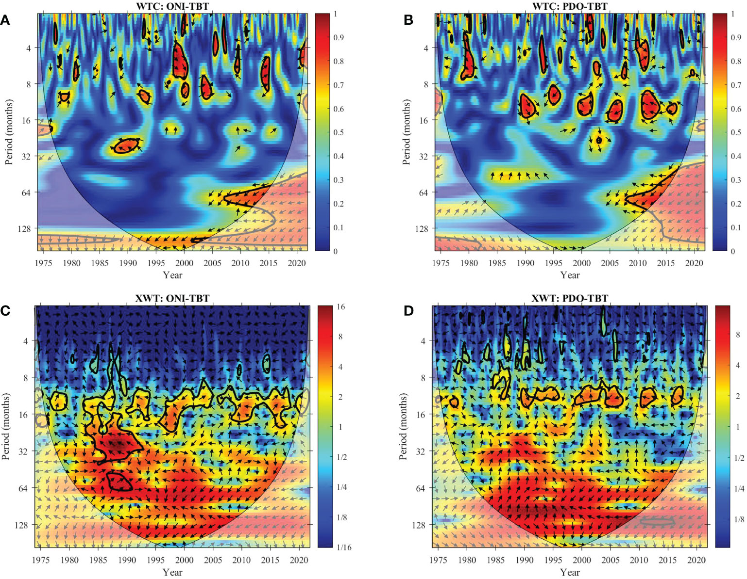
Figure 10 WTC and XWT spectrum of ocean-atmosphere variabilities and the RSL at TBT site. (A, B) are the WTC spectrums of ONI-TBT and PDO-TBT. (C, D) are the XWT spectrums of ONI-TBT and PDO-TBT.

Figures 11A, B shows the WTC results related to ONI, PDO, and RSL at the SPW site. The years of high coherence between ONI and RSL were evident from 2001 to around 2012, in which the period was about 25 months. The arrow pointing to the upper left, ONI is 3/8 periods (about 9 months) ahead of RSL (Figure 11A). PDO and RSL are highly correlated in 1999-2003, 2005-2007, and 2011-2017, with periods of roughly 8 to 16 months. The phase angle is roughly 90°-180°, and PDO is 1/4-1/2 period (2-8 months) ahead of the RSL (Figure 11B). Both ONI and PDO showed strong coherence with the RSL, with a coherence coefficient of more than 0.9, during 2005-2015. They are in anti-phase, indicating that ONI and PDO lead the RSL for around 30 months.

FIGURE 11

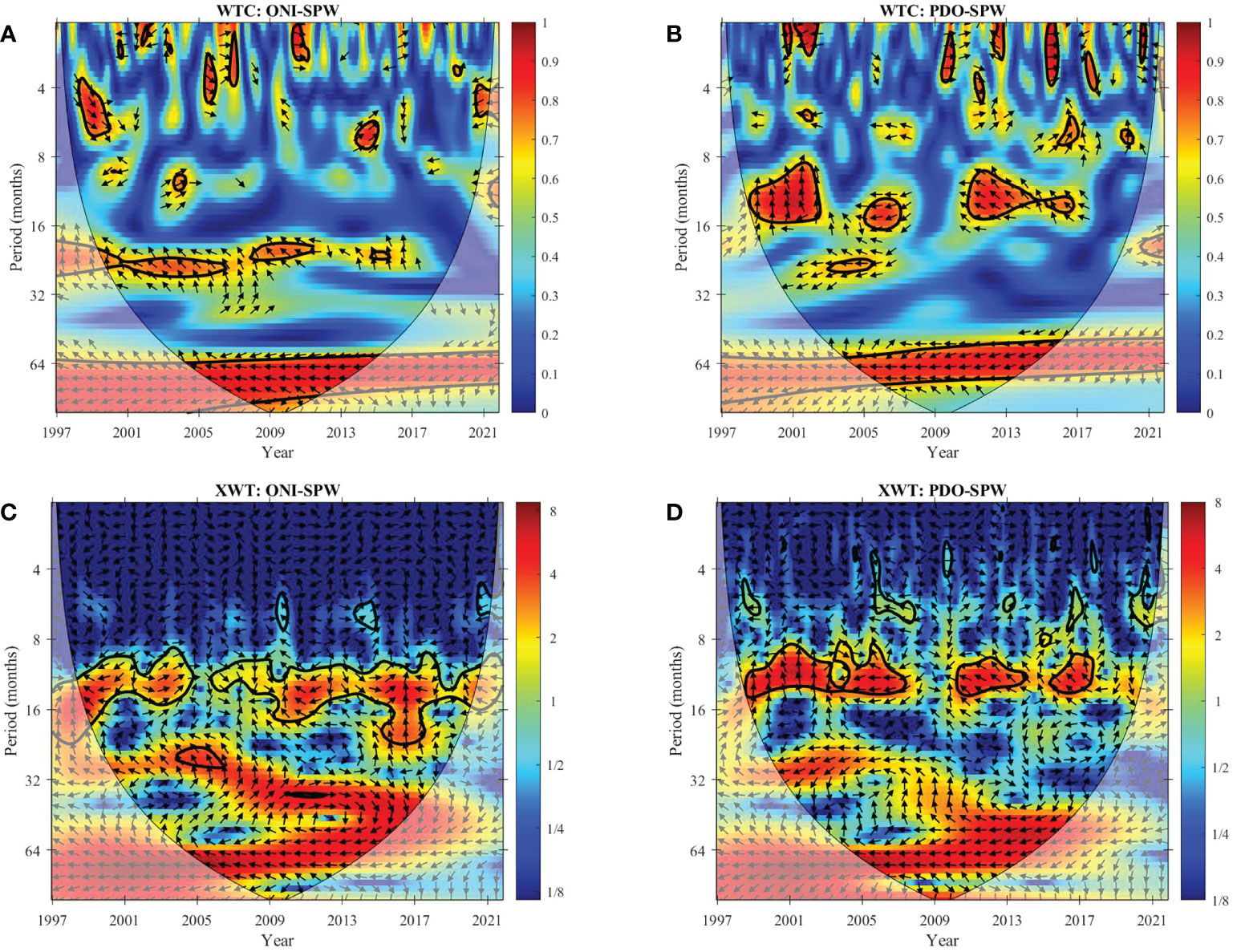
Figure 11 WTC and XWT spectrum of ocean-atmosphere variabilities and the RSL at SPW site. (A, B) are the WTC spectrums of ONI-SPW and PDO-SPW. (C, D) are the XWT spectrums of ONI-SPW and PDO-SPW.

Images (C) and (D) in Figures 9–11 are the XWT spectra between ONI, PDO, and the RSL in all study sites. It can be noticed that both ONI and PDO had a high common period intensity with the RSL at all tide gauge stations throughout the study time scale, with a period of approximately 18-16 months. In addition, when ONI and PDO are highly coherent with RSL, their shared high common power is also significant. This implies that in most cases, the dramatic sea-level changes in Hong Kong lagged behind the dramatic changes in ENSO and PDO that occurred for a period of time.

5. Discussion

5.1. Future trend of RSL in Hong Kong

This research analyzed multi-scale periodicity and non-stationary characteristics of sea-level dynamics through Wavelet Transform and HHT method. Our study shows that the RSL in Hong Kong mainly experienced 2.5 cycles of high-to-low sea-level transition. Although the RSL is subject to periodic declines due to the ocean-atmosphere climate variability, the long-term mean RSL in Hong Kong is generally on the rise. In QUB station, the RSL rose by 1.56mm/yr (1954-2021), which is similar to the previous studies (Ding et al., 2001). They also predicted that the future absolute mean RSL in Hong Kong would be 10cm higher by 2050. However, they did not analyze the spatial heterogeneity of RSLC. The RSLR rates of TBT and SPW stations were 0.44mm/yr (1974-2021) and 0.57mm/yr (1997-2021), respectively, and are slower than the QUB station. Therefore, the future RSL in Hong Kong would be also spatially heterogeneous. The spatial heterogeneity of RSLR in Hong Kong has also been observed by other studies. The tidal patterns in Hong Kong are different in scaling behaviors. The RSLR in different stations exhibits diverse tidal patterns (Zhang and Ge, 2013). Although the RSLR in the Tsim Bei Tsui area is not as fast as that around Victoria Harbor, the Tsim Bei Tsui tide gauge is located in a lower and flatter region that is more prone to coastal flooding than Hong Kong Island or Kowloon.

5.2. Sea-level dynamics and climatic teleconnections

PDO is divided into two phases. In the warm phase, the PDO value is positive, seawater near the equator and the northeast Pacific Ocean has a relatively high sea surface temperature and relatively low pressure, at the same time, the west part of the Pacific Ocean has cooler sea surface temperature and higher pressure. During the cold phase, the situation is reversed, the PDO value is negative, lower sea surface temperatures, and higher atmospheric pressure over the equator and the northeast Pacific Ocean, meanwhile, the western part of the Pacific Ocean would become warmer and has lower pressure. PDO may change before the sea-level change. The specific time of PDO ahead of RSL varies in different years and periods. Climate systems could affect sea-level variation through sea surface wind intensity, pressure, heat transport, and flux (Srinivasu et al., 2017). Other studies demonstrated that interannual and decadal variability of PDO could affect sea-level dynamics in the South China Sea. Averaged sea level anomaly in the South China Sea has a negative correlation with the PDO (r=-0.96). PDO affects and adjusts sea-level dynamics through the propagation of Rossby waves (Cheng et al., 2016). The impact of PDO extends beyond the Pacific Ocean and can even affect the sea level in the Indian Ocean. In the cold phase (warm phase), sea level rise (fall) happens in the tropical Indian Ocean (50°E–80°E; 15°S–5°S) (Deepa et al., 2019).

ENSO is a significant signal of interannual and interdecadal climate change on a global scale (Dieppois et al., 2021). It is a low-latitude sea-air interaction phenomenon characterized by the El Niño-La Niña transition in the ocean and the Southern Oscillation in the atmosphere, affecting the global climate system and sea level (Muis et al., 2018; Timmermann et al., 2018). The changes in RSL in Hong Kong lag the changes of ENSO by 9-16 months. El Niño events are accompanied by a low-pressure state existing in the eastern tropical Pacific. In the equatorial Pacific, the trade winds are weaker than normal, and warm water in the west moves eastward, which results in low sea level in the west part of the Pacific Ocean, including the waters of eastern Hong Kong. During La Niña events, a high-pressure state exists in the eastern tropical Pacific. Easterly trade winds become stronger. More sea surface water is brought westward by westward flow, which may cause high sea level around eastern Hong Kong. The sea level height of the South China Sea is highly correlated with ENSO events (Wu and Chang, 2005).

GMSL is highly correlated with ENSO (timescales > 1.5yr), and moderately correlated with PDO (timescales > 4yr) (Liao and Chao, 2022). In the South China Sea, PDO contributes 72% sea level rise from 1993 to 2012, making the sea level rise 5.0mm/yr which is higher than the rate of GMSL (3.3mm/yr) (Cheng et al., 2016). ENSO events also drive interannual and interdecadal variations in mean as well as extreme sea levels, threatening coastal life and properties (Muis et al., 2018). Therefore, it will be important for future research to consider the impact of the global climate systems on RSL height projection on global or local scales.

5.3. Spatial-temporal heterogeneity of sea-level dynamics in Hong Kong

The periods of RSLC at three tide gauges vary from 125 to 350 months and the time lag of the RSL in three sites affected by ENSO and PDO varies. Moreover, the highly coherent years between ocean-atmosphere climate variability and RSL at the TBT station are short and discontinuous, and the phase angle is relatively diverse (Figures 10A, B). These may reflect the spatial-temporal heterogeneity of sea-level dynamics, which may firstly relate to the location and shape of the coastal shoreline. QUB is located on the channel between Kowloon Peninsula and Hong Kong Island, southeast of Victoria Harbor. SPW is on the southwest open shoreline of Lantau Island. TBT is situated on the bottom of Shenzhen Bay, near the mouth of the Pearl River. Compared with QUB and SPW stations, the location of TBT stations is closer to the northwest part of Hong Kong. This enclosed bay is sheltered from the open sea and more influenced by inland water systems such as freshwater input from the Pearl River and Shenzhen River than by the Pacific current. The east sea area and open sea to the south of Hong Kong, where the QUB and SPW stations are located, are less affected by the inland rivers, and so have a more obvious interaction with the ocean and atmosphere in the tropical Pacific Ocean associated with ENSO and PDO. Secondly, different intensities of anthropogenic activities in these regions have different impacts on the hydrodynamic and morphogenetic processes at three tide gauges (Zhang and Ge, 2013). The SPW station on the southern side of Lantau Island is less affected by human activities than the TBT and QUB stations. TBT may be affected by the urbanization process of Shenzhen and Yuen Long district of Hong Kong, which may change sediment flux, freshwater input, and seawater salinity, while QUB may be affected by reclamation. Thirdly, the heterogeneity of sea-level dynamics may also be affected by the inverted barometer effect caused by differences in air pressure over the sea. The impact of ocean tide and air pressure on sea-level dynamics in Hong Kong is different (Zou et al., 2021). In addition, seabed topography, upwelling, and other natural factors may also cause the heterogeneity of sea-level dynamics in Hong Kong (Hu and Wang, 2016; Xu et al., 2016). Sea-level variations in the South China Sea differ spatially, and temporally. Mean sea level in the South China Sea rose at a rate of 11.3mm/yr between 1993 and 2000 and fell at the rate of 11.8mm/yr over the following five years. The large rise rate occurred in the area from the west of Luzon Island to the east of Vietnam during 1993-2000, while the largest fall rate occurred in the east area off Vietnam during 2001-2005. The heat transfer of the sea surface of South China Sea significantly contributes to sea level height variations (Cheng and Qi, 2007). To understand the sea-level dynamics in such a local area, research on the thermal exchange of the upper layer of seawater should be conducted in Hong Kong. However, the limited resolution of measurements of sea-surface temperature and height from satellites is likely insufficient to examine spatial heterogeneity across a relatively small coastal area such as Hong Kong. Meanwhile, long-term and high-temporal resolution data are not supported by remote sensing data (Cheng and Qi, 2007; Cheng et al., 2016; Vignudelli et al., 2019). More accurate and high-resolution observation data need to be combined with large-scale satellite remote sensing data when studying local or even large-scale sea-level variations.

6. Conclusions

We applied the Wavelet Transform and HHT method to hourly tidal data from three tide gauge stations, the time scale span 68 years, from 1954 to 2021, to investigate the non-stationarity and multi-scale periodicity of Hong Kong RSLC. The main conclusions are as follows:

Firstly, based on the Wavelet Transform, the RSL recorded by QUB, SPW, and TBT tide gauge stations since the day of station setup presents multi-scale periodicity, which is mainly reflected in that the RSL has experienced 2.5 cycles of high to low sea-level transition. The first major period of RSLC is about 350, 250, and 125 months at QUB, TBT, and SPW sites, respectively. When the time scale is 18-20 months, the periodicity of RSL at three stations is obvious. Besides, the RSL also showed significant periodicity when the time scale is 25-50 months in the TBT station.

Secondly, according to EMD results, the RSLC in different regions of Hong Kong have spatio-temporal heterogeneity. The RSL has a similar tendency that first fell, then went through a long-term slow rise, and fell again in recent years, at SPW and QUB stations. They are predicted to fall at an annual rate of 10.6 mm/yr and 0.7 mm/yr in the next several years, respectively. At the TBT station, the RSL fell before 1996 and rose until 2021. It may continuously rise by 3.6 mm/yr for the next several years. RSLR results from combined contributions of sea-level rise and local vertical land movement.

Thirdly, the tidal amplitude related to ENSO and PDO can be reflected by the Hilbert spectrum. The effect of ENSO events and PDO on the RSL around Hong Kong is spatial-temporal heterogeneous. The changes in RSL in Hong Kong lag the changes of ENSO and PDO many of the time. This time lag varies from about 6-30 months, depending on the period. The differences in sea-level dynamics in different parts of Hong Kong are likely because the western sea of Hong Kong is more influenced by inland rivers and interacts less with currents and heat transfer on the upper layer of the western Pacific.

These findings will help to understand the mechanism of sea-level dynamics and its relationship with climate teleconnection, providing more information for Hong Kong to cope with global climate change and RSLR.

Data availability statement

The raw data supporting the conclusions of this article will be made available by the authors, without undue reservation.

Author contributions

XL: Formal analysis, investigation, data curation, visualization, writing-original draft. YL: Writing-review & editing. RW: Writing-review & editing. GL: Writing-review&editing. NK: Writing-review & editing. RL: Writing-review & editing. HS: Writing-review & editing. SW: Writing-review & editing. HZ: Conceptualization, supervision, funding acquisition, writing-review & editing. All authors contributed to the article and approved the submitted version.

Funding

This study was jointly supported by the Research Grants Council (RGC) of Hong Kong, China (HKU27602020, HKU17613022, HKU14605917), the National Natural Science Foundation of China (42022061 and 42071390) and the University of Hong Kong (202011159112).

Acknowledgments

The authors would like to thank the Hong Kong Observatory for providing tidal and precipitation data, National Oceanic and Atmospheric Administration (NOAA) for providing ENSO index and PDO index data.

Conflict of interest

The authors declare that the research was conducted in the absence of any commercial or financial relationships that could be construed as a potential conflict of interest.

Publisher’s note

All claims expressed in this article are solely those of the authors and do not necessarily represent those of their affiliated organizations, or those of the publisher, the editors and the reviewers. Any product that may be evaluated in this article, or claim that may be made by its manufacturer, is not guaranteed or endorsed by the publisher.

References

Bunge L., Clarke A. J., et al. (2009). A verified estimation of the El Niño index Niño-3.4 since 1877. J. Clim. 22, 3979–3992.

Google Scholar

Cazenave A., Henry O., Munier S., Delcroix T., Gordon A., Meyssignac B., et al. (2012). Estimating ENSO influence on the global mean sea level 1993–2010. Mar. Geodesy 35, 82–97. doi: 10.1080/01490419.2012.718209

CrossRef Full Text | Google Scholar

Cheng X., Qi Y. (2007). Trends of sea level variations in the south China Sea from merged altimetry data. Global Planetary Change 57, 371–382. doi: 10.1016/j.gloplacha.2007.01.005

CrossRef Full Text | Google Scholar

Cheng X., Xie S.-P., Du Y., Wang J., Chen X., Wang J. (2016). Interannual-to-decadal variability and trends of sea level in the south China Sea. Climate Dynamics 46, 3113–3126. doi: 10.1007/s00382-015-2756-1

CrossRef Full Text | Google Scholar

Chen X., Zhang X., Church J. A., Watson C. S., King M. A., Monselesan D., et al. (2017). The increasing rate of global mean sea-level rise during 1993–2014. Nat. Climate Change 7, 492–495. doi: 10.1038/nclimate3325

CrossRef Full Text | Google Scholar

Deepa J., Gnanaseelan C., Mohapatra S., Chowdary J., Karmakar A., Kakatkar R., et al. (2019). The tropical Indian ocean decadal sea level response to the pacific decadal oscillation forcing. Climate Dynamics 52, 5045–5058. doi: 10.1007/s00382-018-4431-9

CrossRef Full Text | Google Scholar

Dieppois B., Capotondi A., Pohl B., Chun K. P., Monerie P.-A., Eden J. (2021). ENSO diversity shows robust decadal variations that must be captured for accurate future projections. Commun. Earth Environ. 2, 1–13. doi: 10.1038/s43247-021-00285-6

CrossRef Full Text | Google Scholar

Ding X., Chao J., Zheng D., Chen Y. (2001). Long-term sea-level changes in Hong Kong from tide-gauge records. J. Coast. Res. 17 (3), 749–754.

Google Scholar

Dixon M. J., Tawn J. A. (1999). The effect of non-stationarity on extreme sea-level estimation. J. R. Stat. Society: Ser. C (Applied Statistics) 48, 135–151. doi: 10.1111/1467-9876.00145

CrossRef Full Text | Google Scholar

Drago A., Boxall S. R. (2002). Use of the wavelet transform on hydro-meteorological data. Phys. Chem. Earth Parts A/B/C 27, 1387–1399. doi: 10.1016/S1474-7065(02)00076-1

CrossRef Full Text | Google Scholar

Duffy D. G. (2004). The application of Hilbert–Huang transforms to meteorological datasets. J. Atmospheric Oceanic Technol. 21, 599–611. doi: 10.1175/1520-0426(2004)021<0599:TAOHTT>2.0.CO;2

CrossRef Full Text | Google Scholar

El-Askary H., Sarkar S., Chiu L., Kafatos M., El-Ghazawi T. (2004). Rain gauge derived precipitation variability over Virginia and its relation with the El nino southern oscillation. Adv. Space Res. 33, 338–342. doi: 10.1016/S0273-1177(03)00478-2

CrossRef Full Text | Google Scholar

Ezer T., Atkinson L. P., Corlett W. B., Blanco J. L. (2013). Gulf stream's induced sea level rise and variability along the US mid-Atlantic coast. J. Geophysical Research: Oceans 118, 685–697. doi: 10.1002/jgrc.20091

CrossRef Full Text | Google Scholar

Goddard P., Yin J., Griffies S., Zhang S. (2015). An extreme event of sea-level rise along the northeast coast of north America in 2009–2010. Nat. Commun. 6, 6346. doi: 10.1038/ncomms7346

PubMed Abstract | CrossRef Full Text | Google Scholar

Gregory J. M., Griffies S. M., Hughes C. W., Lowe J. A., Church J. A., Fukimori I., et al. (2019). Concepts and terminology for sea level: Mean, variability and change, both local and global. Surveys Geophysics 40, 1251–1289. doi: 10.1007/s10712-019-09525-z

CrossRef Full Text | Google Scholar

Grinsted A., Moore J. C., Jevrejeva S. (2004). Application of the cross wavelet transform and wavelet coherence to geophysical time series. Nonlinear processes geophysics 11, 561–566. doi: 10.5194/npg-11-561-2004

CrossRef Full Text | Google Scholar

Hamlington B., Leben R., Strassburg M., Nerem R., Kim K. Y. (2013). Contribution of the pacific decadal oscillation to global mean sea level trends. Geophysical Res. Lett. 40, 5171–5175. doi: 10.1002/grl.50950

CrossRef Full Text | Google Scholar

Huang N. E. (2014). Hilbert-Huang Transform and its applications. Second Edition. (Singapore: World Scientific Publishing Co. Pte. Ltd.)

Google Scholar

Hu J., Wang X. H. (2016). Progress on upwelling studies in the China seas. Rev. Geophysics 54, 653–673. doi: 10.1002/2015RG000505

CrossRef Full Text | Google Scholar

Idier D., Bertin X., Thompson P., Pickering M. D. (2019). Interactions between mean sea level, tide, surge, waves and flooding: mechanisms and contributions to sea level variations at the coast. Surveys Geophysics 20 (4), 817–824. doi: 10.1016/j.ymssp.2005.09.011

CrossRef Full Text | Google Scholar

Junsheng C., Dejie Y., Yu Y. (2006). Research on the intrinsic mode function (IMF) criterion in EMD method. Mech. Syst. Signal. Process. 20 (4), 817–824. doi: 10.1016/j.ymssp.2005.09.011

CrossRef Full Text | Google Scholar

Karamperidou C., Engel V., Lall U., Stabenau E., Smith T. J. (2013). Implications of multi-scale sea level and climate variability for coastal resources. Regional Environ. Change 13, 91–100. doi: 10.1007/s10113-013-0408-8

CrossRef Full Text | Google Scholar

Kirwan M. L., Megonigal J. P. (2013). Tidal wetland stability in the face of human impacts and sea-level rise. Nature 504, 53–60. doi: 10.1038/nature12856

PubMed Abstract | CrossRef Full Text | Google Scholar

Kulp S. A., Strauss B. H. (2019). New elevation data triple estimates of global vulnerability to sea-level rise and coastal flooding. Nat. Commun. 10, 1–12. doi: 10.1038/s41467-019-12808-z

PubMed Abstract | CrossRef Full Text | Google Scholar

Latif M., Keenlyside N. S. (2009). El Niño/Southern oscillation response to global warming. Proc. Natl. Acad. Sci. 106, 20578–20583. doi: 10.1073/pnas.0710860105

CrossRef Full Text | Google Scholar

Lee B., Wong W., Woo W. (2010). Sea-Level rise and storm surge–impacts of climate change on Hong kong. HKIE civil division conference. Hong Kong Observatory Hong Kong, 12–14. Available at: https://www.hko.gov.hk/tc/publica/reprint/files/r915.pdf.

Google Scholar

Lelieveld J., Proestos Y., Hadjinicolaou P., Tanarhte M., Tyrlis E., Zittis G. (2016). Strongly increasing heat extremes in the middle East and north Africa (MENA) in the 21st century. Climatic Change 137, 245–260. doi: 10.1007/s10584-016-1665-6

CrossRef Full Text | Google Scholar

Liao T.-J., Chao B. F. (2022). Global mean Sea level variation on interannual–decadal timescales: Climatic connections. Remote Sens. 14, 2159. doi: 10.3390/rs14092159

CrossRef Full Text | Google Scholar

Lovelock C. E., Feller I. C., Reef R., Hickey S., Ball M. C. (2017). Mangrove dieback during fluctuating sea levels. Sci. Rep. 7, 1–8. doi: 10.1038/s41598-017-01927-6

PubMed Abstract | CrossRef Full Text | Google Scholar

Mantua N. J., Hare S. R. (2002). The pacific decadal oscillation. J. oceanography 58, 35–44. doi: 10.1023/A:1015820616384

CrossRef Full Text | Google Scholar

Ma P., Wang W., Zhang B., Wang J., Shi G., Huang G., et al. (2019). Remotely sensing large-and small-scale ground subsidence: A case study of the guangdong–Hong Kong–Macao greater bay area of China. Remote Sens. Environ. 232, 111282. doi: 10.1016/j.rse.2019.111282

CrossRef Full Text | Google Scholar

Mcphaden M. J., Busalacchi A. J., Cheney R., Donguy J. R., Gage K. S., Halpern D., et al. (1998). The tropical ocean-global atmosphere observing system: A decade of progress. J. Geophysical Res.: Oceans 103, 14169–14240. doi: 10.1029/97JC02906

CrossRef Full Text | Google Scholar

Melet A., Meyssignac B., Almar R., LE Cozannet G. (2018). Under-estimated wave contribution to coastal sea-level rise. Nat. Climate Change 8, 234–239. doi: 10.1038/s41558-018-0088-y

CrossRef Full Text | Google Scholar

Metropolis N., Ulam S. (1949). The monte carlo method. J. Am. Stat. Assoc. 44, 335–341. doi: 10.1080/01621459.1949.10483310

PubMed Abstract | CrossRef Full Text | Google Scholar

Morlet J., Arens G., Fourgeau E., Glard D. (1982). Wave propagation and sampling theory–part I: Complex signal and scattering in multilayered media. Geophysics 47, 203–221. doi: 10.1190/1.1441328

CrossRef Full Text | Google Scholar

Muis S., Haigh I. D., Guimarães Nobre G., Aerts J. C., Ward P. J. (2018). Influence of El niño-southern oscillation on global coastal flooding. Earth's Future 6, 1311–1322. doi: 10.1029/2018EF000909

CrossRef Full Text | Google Scholar

Passeri D. L., Hagen S. C., Medeiros S. C., Bilskie M. V., Alizad K., Wang D. (2015). The dynamic effects of sea level rise on low-gradient coastal landscapes: A review. Earth's Future 3, 159–181. doi: 10.1002/2015EF000298

CrossRef Full Text | Google Scholar

Roe G. H., Baker M. B., Herla F. (2017). Centennial glacier retreat as categorical evidence of regional climate change. Nat. Geosci. 10, 95–99. doi: 10.1038/ngeo2863

CrossRef Full Text | Google Scholar

Royston P., White I. R. (2011). Multiple imputation by chained equations (MICE): implementation in stata. J. Stat. software 45, 1–20. doi: 10.18637/jss.v045.i04

CrossRef Full Text | Google Scholar

Scafetta N. (2014). Multi-scale dynamical analysis (MSDA) of sea level records versus PDO, AMO, and NAO indexes. Climate dynamics 43, 175–192. doi: 10.1007/s00382-013-1771-3

CrossRef Full Text | Google Scholar

Schneider N., Cornuelle B. D. (2005). The forcing of the pacific decadal oscillation. J. Climate 18, 4355–4373. doi: 10.1175/JCLI3527.1

CrossRef Full Text | Google Scholar

Sreedevi V., Adarsh S., Nourani V. (2022). Multiscale coherence analysis of reference evapotranspiration of north-western Iran using wavelet transform. J. Water Climate Change 13, 505–521. doi: 10.2166/wcc.2021.379

CrossRef Full Text | Google Scholar

Srinivasu U., Ravichandran M., Han W., Sivareddy S., Rahman H., Li Y., et al. (2017). Causes for the reversal of north Indian ocean decadal sea level trend in recent two decades. Climate Dynamics 49, 3887–3904. doi: 10.1007/s00382-017-3551-y

CrossRef Full Text | Google Scholar

Strauss B. H., Kulp S. A., Rasmussen D., Levermann A. (2021). Unprecedented threats to cities from multi-century sea level rise. Environ. Res. Lett. 16, 114015. doi: 10.1088/1748-9326/ac2e6b

CrossRef Full Text | Google Scholar

Tam N. F., Wong Y.-S., Lu C., Berry R. (1997). Mapping and characterization of mangrove plant communities in Hong kong. In: Wong Y. S., Tam N.F. Y. (eds.) Asia-Pacific Conference on Science and Management of Coastal Environment. Developments in Hydrobiology (Dordecht: Springer) 123, 25–37. doi: 10.1007/978-94-011-5234-1_4

CrossRef Full Text | Google Scholar

Timmermann A., An S.-I., Kug J.-S., Jin F.-F., Cai W., Capotondi A., et al. (2018). El Niño–southern oscillation complexity. Nature 559, 535–545. doi: 10.1038/s41586-018-0252-6

PubMed Abstract | CrossRef Full Text | Google Scholar

Torrence C., Compo G. P. (1998). A practical guide to wavelet analysis. Bull. Am. Meteorological Soc. 79, 61–78. doi: 10.1175/1520-0477(1998)079<0061:APGTWA>2.0.CO;2

CrossRef Full Text | Google Scholar

Turki I., Baulon L., Massei N., Laignel B., Costa S., Fournier M., et al. (2020). A nonstationary analysis for investigating the multiscale variability of extreme surges: case of the English channel coasts. Natural Hazards Earth System Sci. 20, 3225–3243. doi: 10.5194/nhess-20-3225-2020

CrossRef Full Text | Google Scholar

Vignudelli S., Birol F., Benveniste J., Fu L.-L., Picot N., Raynal M., et al. (2019). Satellite altimetry measurements of sea level in the coastal zone. Surveys geophysics 40, 1319–1349. doi: 10.1007/s10712-019-09569-1

CrossRef Full Text | Google Scholar

Wang J., Gao W., XU S., Yu L. (2012). Evaluation of the combined risk of sea level rise, land subsidence, and storm surges on the coastal areas of shanghai, China. Climatic Change 115, 537–558. doi: 10.1007/s10584-012-0468-7

CrossRef Full Text | Google Scholar

Wong W., Li K., Yeung K. (2003). Long term sea level change in Hong Kong. Hong Kong Meteorological Soc. Bull. 13, 24–40.

Google Scholar

Wu C. R., Chang C. W. J. (2005). Interannual variability of the south China Sea in a data assimilation model. Geophysical Res. Lett. 32 (17). doi: 10.1029/2005GL023798

CrossRef Full Text | Google Scholar

Xu Z., Liu K., Yin B., Zhao Z., Wang Y., Li Q. (2016). Long-range propagation and associated variability of internal tides in the s outh c hina s ea. J. Geophysical Research: Oceans 121, 8268–8286. doi: 10.1002/2016JC012105

CrossRef Full Text | Google Scholar

Zhang Y., Ge E. (2013). Temporal scaling behavior of sea-level change in Hong Kong–multifractal temporally weighted detrended fluctuation analysis. Global Planetary Change 100, 362–370. doi: 10.1016/j.gloplacha.2012.11.012

CrossRef Full Text | Google Scholar

Zou F., Tenzer R., Fok H. S., Meng G., Zhao Q. (2021). The sea-level changes in Hong Kong from tide-gauge records and remote sensing observations over the last seven decades. IEEE J. Selected Topics Appl. Earth Observations Remote Sens. 14, 6777–6791. doi: 10.1109/JSTARS.2021.3087263

CrossRef Full Text | Google Scholar