Efficient spatial kelp biomass estimations using acoustic methods

Kelp forests are the largest vegetated marine ecosystem on earth, but vast areas of their distribution remain unmapped and unmonitored. Efficient and cost-effective methods for measuring the standing biomass of these ecosystems are urgently needed for coastal mapping, ocean accounting and sustainable management of wild harvest. Here we show how widely available acoustic equipment on vessels can be used to perform robust and large-scale (kilometer) quantifications of kelp biomass which can be used in assessments and monitoring programs. We demonstrate how to interpret echograms from acoustic systems into point estimates of standing biomass in order to create spatial maps of biomass distribution. We also explore what environmental conditions are suitable for acoustic measures. This has direct application for blue carbon accounting, coastal monitoring, management of wild seaweed harvest and the protection and conservation of marine habitats supporting high biodiversity.

Introduction

Shallow water coastal zones are among the most productive oceanic environments and display a complex variety of benthic habitats. A better understanding of the distribution and abundance of these habitats is vital to quantify the function of marine ecosystems, the ecological drivers of change, and how to manage these ecosystems and associated resources sustainable way (Norderhaug et al., 2020a; Norderhaug et al., 2020b; St-Pierre and Gagnon, 2020). Kelp forests are the largest vegetated ecosystem in the world (Duarte et al., 2022) and are key drivers of productivity in shallow marine habitats (Pessarrodona et al., 2022), and large parts of their distribution are unmapped, or rely on coarse species distribution models using limited data (Wernberg et al., 2019; Assis et al., 2022). This is especially true for kelps that form subsurface canopies, which comprise about a third of all kelp species, and unlike surface canopy forming kelps cannot be reliably mapped across their depth range using satellites or drones (Mora-Soto et al., 2020; Cavanaugh et al., 2021). Although high resolution distribution maps of kelp forests are increasingly available in some regions, maps of standing biomass remain rare. There is an urgent need for efficient monitoring tools of kelp forests (Duffy et al., 2019), to ensure their sustainable management, increase the understanding of their blue carbon potential and other ecosystem services, and assess impacts from global change including warming (Pörtner et al., In Press; Wernberg et al., 2016; Filbee-Dexter and Wernberg, 2020).

A variety of methods and field observations are used to assess and monitor kelp distribution, abundance and biomass, including physical sampling by diving or snorkelling, underwater photographs or video, aerial photographs, historical records (Bennion et al., 2019), and newer remote methods such as laser imaging, detection, and ranging (LiDAR) and acoustics. In Norway, physical sampling and underwater cameras are used to monitor the condition of kelp forests, the impacts of kelp harvesting and rates of recovery; however, while intense diver and underwater camera surveys can provide highly accurate data (van Son et al., 2020) they are very challenging and time consuming to undertake. Some of the logistic challenges of these physical sampling methods include difficult wave, currents and weather conditions, rocky substrata, inaccessible habitat areas, labour-intensive sampling procedures and time-consuming video analysis are. In recent years there has been an increased focus on how to improve species distribution models by using remote sensing. For example, both single- and multibeam acoustics as well as LiDAR can improve the prediction accuracy of kelp distribution and abundance (Young et al., 2015; Bennion et al., 2019; Norderhaug et al., 2021). Efficient methods such as these that cover large spatial scales are needed to produce a better global understanding of status and change in kelp forests.

Standing kelp biomass can provide essential information on kelp forest function, as it captures elements of kelp productivity, habitat provision and condition. In northern Europe, Laminaria hyperborea is regarded as one of the most important kelp species, both ecologically and commercially (Norderhaug et al., 2021). L. hyperborea forms dense forests in wave exposed areas along the Norwegian coast providing a high production and habitat for a range of marine organisms. Each square metre of these ‘blue forests’ may host as many as 100 000 crustaceans, mussels, echinoderms and polychaetes, which comprise the main food sources for many coastal fish stocks, marine mammals and seabirds using the forests as feeding grounds and/or nursery habitat (Norderhaug et al., 2005; Norderhaug et al., 2020a). L. hyperborea forests with high standing biomass tend to have higher productivity than low-growing forests (Pessarrodona et al., 2018) and create more vertical habitat structure, with more space for epiphytes on their stipe and better protection for fish species. The forests also supply organic matter to neighbouring communities such as deep-sea ecosystems through the export of detached biomass (Filbee-Dexter et al., 2018). This pathways can contribute to carbon sequestration due to burial and long-term storage of kelp matter in deep-sea sediments (Filbee-Dexter et al., 2018; Gundersen et al., 2021). One barrier for understanding the significance of this pathway in a lack of knowledge of spatial distribution and biomass of forest forming kelps (Krause-Jensen et al., 2018). In Norway the annual harvesting of L. hyperborea is primarily managed by estimating standing biomass in open harvest areas using extensive annual surveys with underwater cameras (Steen et al., 2016), and amounts to approximately 150 000 tonnes, depending on available harvest fields, seabed conditions and other environmental factors (Norderhaug et al., 2021), and

In this study we tested echo sounding as a tool to estimate kelp biomass in surveys along the northwest coast of Norway. We analysed the amount of reflected energy (echo intensity) of kelp forests recorded from echograms and compared these with biomass estimates derived from a well-established method that includes physical sampling and video analysis, as described in van Son et al., 2020. We used the relationship between these known standing biomass data and the backscatter signals to develop a model to estimate standing biomass and assesses the potential of this tool for kelp distribution models at large scales.

Data and methods

Study areas

The study was performed on the northwest coast of Norway in the areas of Vikna and Helgeland in June 2021 (Figure 1). The study area is in the outer archipelagos and exposed to waves from the Norwegian sea to the west and a semidiurnal tide with average amplitude of approximately 1.5 m (http://sehavniva.no). The study area stretches from 64° 45’ to 65° 33’ northern latitude in the coastal areas of the counties of Trøndelag and Nordland. This area has been previously surveyed, and kelp forests dominates in the shallowest parts interspersed with deeper, less vegetated beds of sand and gravel (Steen et al., 2016; Norderhaug et al., 2020a; Steen, 2020; Norderhaug et al., 2021). The canopy forming kelp species L. hyperborea dominates the most wave exposed western areas, whereas the prostrate kelp species Saccharina latissima tends to dominate more in the sheltered, eastern parts. L. hyperborea harvesting trials have been performed by kelp trawlers at specific sectors in the area during the 2010s and the effect and reversibility of this activity have been duly addressed by studies in the past (Steen et al., 2016; Norderhaug et al., 2020a; Steen, 2020, Steen et al., 2020).

FIGURE 1

Figure 1 The study area on the northwest coast of Norway (as black dots in the small map). Stations at Vikna in the south (in dark green) and Helgeland to the north (in dark blue).

Biological data collection and video sampling

Video observations of kelp biomass were made by using two different camera modules deployed from a boat at the same sites as the echosounder recordings. A underwater camera connected with a live cable (UVS 5080, 700 TVL) and a diving camera (Paralenz Vaquita, 4K) strapped to and facing in the same direction as the former (Figure 2). Both camera modules were equipped with built-in depth sensors, sensitive to the nearest 0.1 m. At each site, the cameras were lowered onto the seabed to record the height and density of the L. hyperborea vegetation, if present (Steen et al., 2016). The average height of the L. hyperborea canopy was measured using the difference between the depth sensor readings when the camera was moved vertically from touching the seabed to hovering the top of the kelp fronds (Steen et al., 2016). Density estimates were made by counting the number of L. hyperborea canopy plants per m² (using the field of view and stipe diameter for scale) from horizontal camera views beneath the kelp canopy lamina layer (Figure 3). The diameter of the lower stipe portions of kelp plants is correlated with their height and this relationship is known from previous collections of kelp plants (Steen et al., 2016, Steen et al., 2020). If kelp plant numbers were high and frond height low, density was estimated as groups (e.g., 10, 12.5, 15, 20 kelp plants per m²). Biomass density estimates (in kg FW m^-2) were obtained by converting the canopy height measurements to plant weight (in kg FW per kelp plant) through a conversion formula established from previous collections of kelp plants and multiply it with the canopy density estimates (in kelp plants per m²) as described in van Son et al. (2020). The accuracy of the height and density method in estimating biomass has been validated using diver biomass collections from 0.25 m² quadrats from the same area (van Son et al. (2020).

FIGURE 2

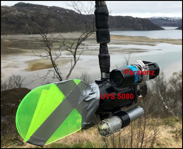
Figure 2 The two camera modules used for video recording. The HD Paralenz camera strapped to the live UVS 5080 camera.

FIGURE 3

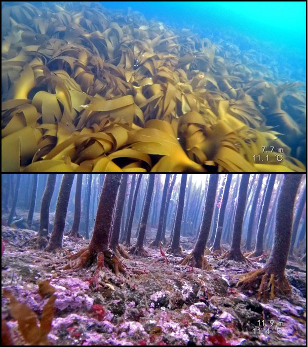
Figure 3 The canopy forming kelp Laminaria hyperborea viewed from above and beneath the lamina layer at the Helgeland area in Nordland.

Acoustic surveys

In this survey a dual-frequency system was used in order to assist both the bottom detection and biomass estimation. Previous studies addressing remote sensing and abundance estimates of kelps has favoured frequencies ranging from 38 to 200kHz (Kjerstad et al., 1995; Woll et al., 1999; Blight et al., 2011; Minami et al., 2014; Shao et al., 2017; Shao et al., 2019). In this survey both the 38kHz and 120kHz transducers were used during acquisition. A total of 319 stations were registered using echosounder during the field work.

Echo sounder data was collected using Simrad EK60 scientific echo sunder with hull mounted split beam transducers ES38B and ES120-7C. The system was calibrated according to standard procedures using a tungsten carbide 57.2 mm calibration sphere prior to the survey (Foote, 1987; Ona, 1999). The echo sounder was set up in a continuous wave (CW) mode with a ping interval of 0.10 s and a range of 50 m for both transducers. Pulse duration of 0.256 ms and transmit power of 250 W was chosen for the 120 kHz transducer while the 38 kHz transducer was set up with pulse duration 0.512 ms and transmit power 800 W. The recording of data was done simultaneously as the video observation for each station. Due to the placement of the camera on a spear at the bow of the boat, and the mounting of the transducers on the hull, the samples are taken approximately 5-8 meters apart depending on the direction of the current.

Processing and interpretation

The acquired data were processed using the processing software KORONA utilizing the processing modules presented in Table 1:

TABLE 1

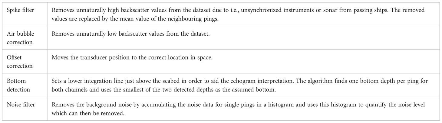
Table 1 Processing modules used in the processing software KORONA.

The processed data were analysed using a standard interpretation procedure for acoustic abundance estimation that involved manual suppression of noise and definition of an integration area that encompass all echoes reflected from the targeted kelp forests (Kjerstad et al., 1995; Blight et al., 2011). The data were interpreted in the echo sounder interpretation software Large Scale Survey System (LSSS) (Figure 4). The interpretation process involved a manual inspection of all datasets in order to quality check the data and to exclude any data which did not contain relevant information or were corrupted. After this, the regions on the echogram that contained kelp forest were defined and designated to an interpretation category using an upper and lower integration line. Unwanted backscatter caused by fish, instruments or other damaging artifacts was removed in order to distinguish the echo caused by the kelp vegetation. The interpreted regions were then sorted in bins containing 100 pings each and the nautical area backscatter coefficient (NASC) was calculated by the interpretation software. The NASC is a scaled version of the s_a-value, and is an important parameter in fisheries acoustics. It is a measure of the energy that is returned from the interval between two integration lines, and is implemented in most echo-integration software (MacLennan, 2002; MacLennan and Simmonds, 2005). The s_a-value is dimensionless but as it is important to indicate the scaling when quoting numerical values, it has been given m² m^-2 as the basic SI unit. The conversion formula for NASC is defined as NASC=4π(1852)²s_a and the resulting NASC unit is thus m² nmi^-2 as defined in MacLennan & Simmonds (2005). In the LSSS software the NASC was averaged in each bin before the values were stored to a database. This was done to be able to address the temporal variations in NASC due to varying noise, orientation, and data artifacts. In this study the database was then scrutinized and compared to the existing biomass density estimates from video analysis for each station using simple statistical tools in order to establish a correlation of the two quantities.

FIGURE 4

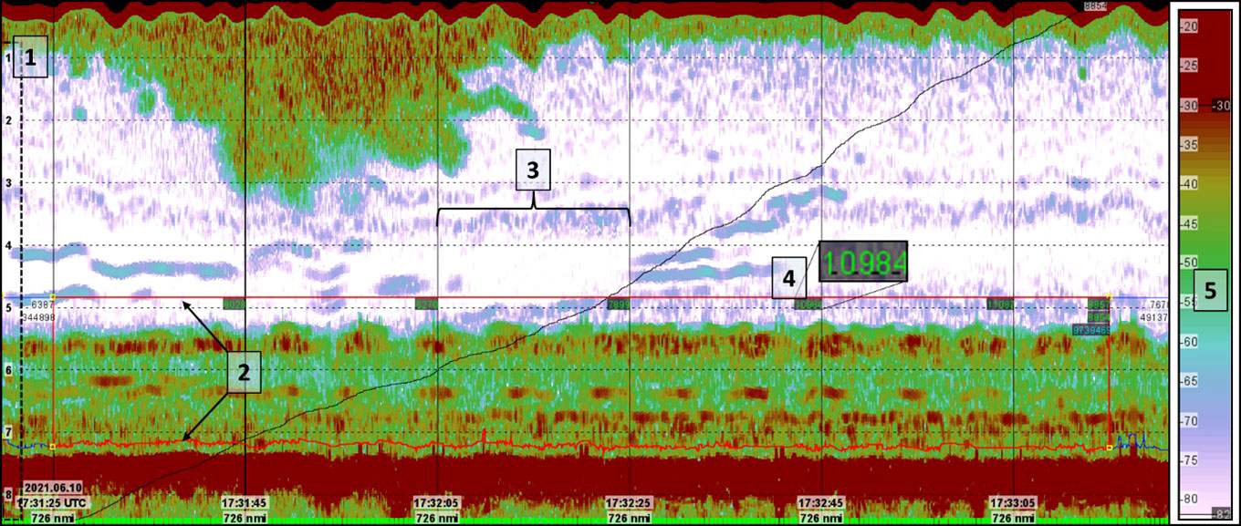
Figure 4 Example of echogram as viewed in the LSSS software. The acoustic data displayed are collected from Vikna station 136. 1) Vertical depth markers measured from the transducer acoustically. 2) Lower and upper integration lines define a region from which the nautical area backscatter coefficient (NASC-value) of the kelp forest is calculated. 3) Vertical lines on the echogram divide the pings into 100-ping segments. 4) NASC-value for each 100-ping bin is displayed directly in the echogram and written to a database. 5) Colour bar showing the volumetric backscatter strength (S_V) with a lower noise threshold (-82dB) and an upper threshold (-35dB).

Results

A total of 329 acquisition points was included in this survey, each stored as a separate dataset. A biomass density estimation for each station was carried out using the method described in van Son et al. (2020). Each of the acoustic datasets were quality checked, and parts of the echograms that were deemed not to contain usable data due to extensive noise, lack of reflections or poor data quality were excluded from further scrutinizing (Figure 5A). Of the total dataset, 31 stations were discarded after data quality check due to lack of usable data. The echograms from the remaining 298 stations were of such quality that a consecutive set of 100 accepted pings were possible to extract and were used in further investigations. The raw echograms were processed using several modules in the KORONA processing package as presented in Table 1. The selected modules were not essential in order to scrutinize the data but ensured a “best practice” approach to interpreting data. The modules aided the interpretation by removing unwanted background noise and spikes and generated bottom detections on the echograms. The lower integration line was set by the aid of the bottom detection algorithm where possible, usually for stations below approximately 10 meters depth. In order to establish a robust model to relate the NASC-value to the biomass of L. hyperborea we used the 120kHz channel. The echograms from the 38kHz channel displayed a large amount of backscatter in the water column, which made it challenging to differentiate the kelp from the background signal as seen in Figure 6. The benefits of using a higher frequency channel was also addressed by Blight et al. (2011), who preferred the cleanliness of the 200kHz channel over the 38kHz channel in their extensive study.

FIGURE 5

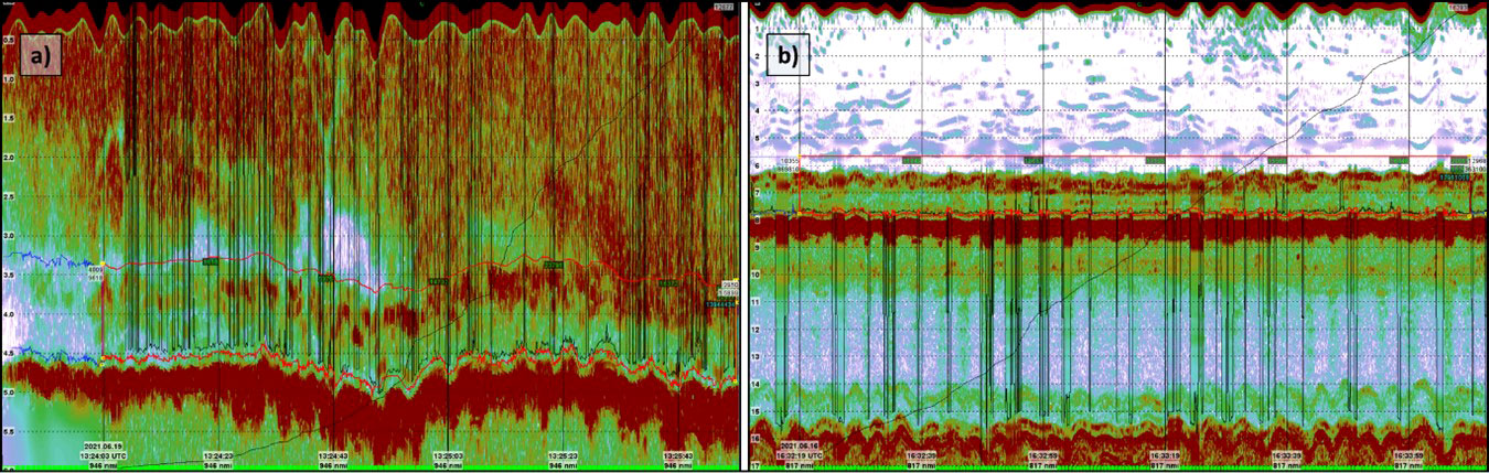
Figure 5 Examples of settings where the bottom detection fails. The black lines show the result of the bottom detection in the pre-processor KORONA, the lower red line is the manually set lower integration line. (A) Echogram from Helgeland station 4 where shallow air bubbles cause the algorithm to fluctuate between the actual seabed and the near field. (B) Echogram from Vikna station 391 where the algorithm fluctuates between the actual seabed and the 2nd echo.

FIGURE 6

Figure 6 Echograms from Helgeland station 152. (A) 38kHz data, (B) 120kHz data. The 120kHz echogram is clearly a lot cleaner, making the detection and mapping of the kelp forest much easier for the interpreter.

The resulting cross plot (Figure 7A) shows a consistent relationship between the estimated kelp biomass and the acoustically derived NASC-values for the 298 stations yielded by the linear least squares model:

FIGURE 7

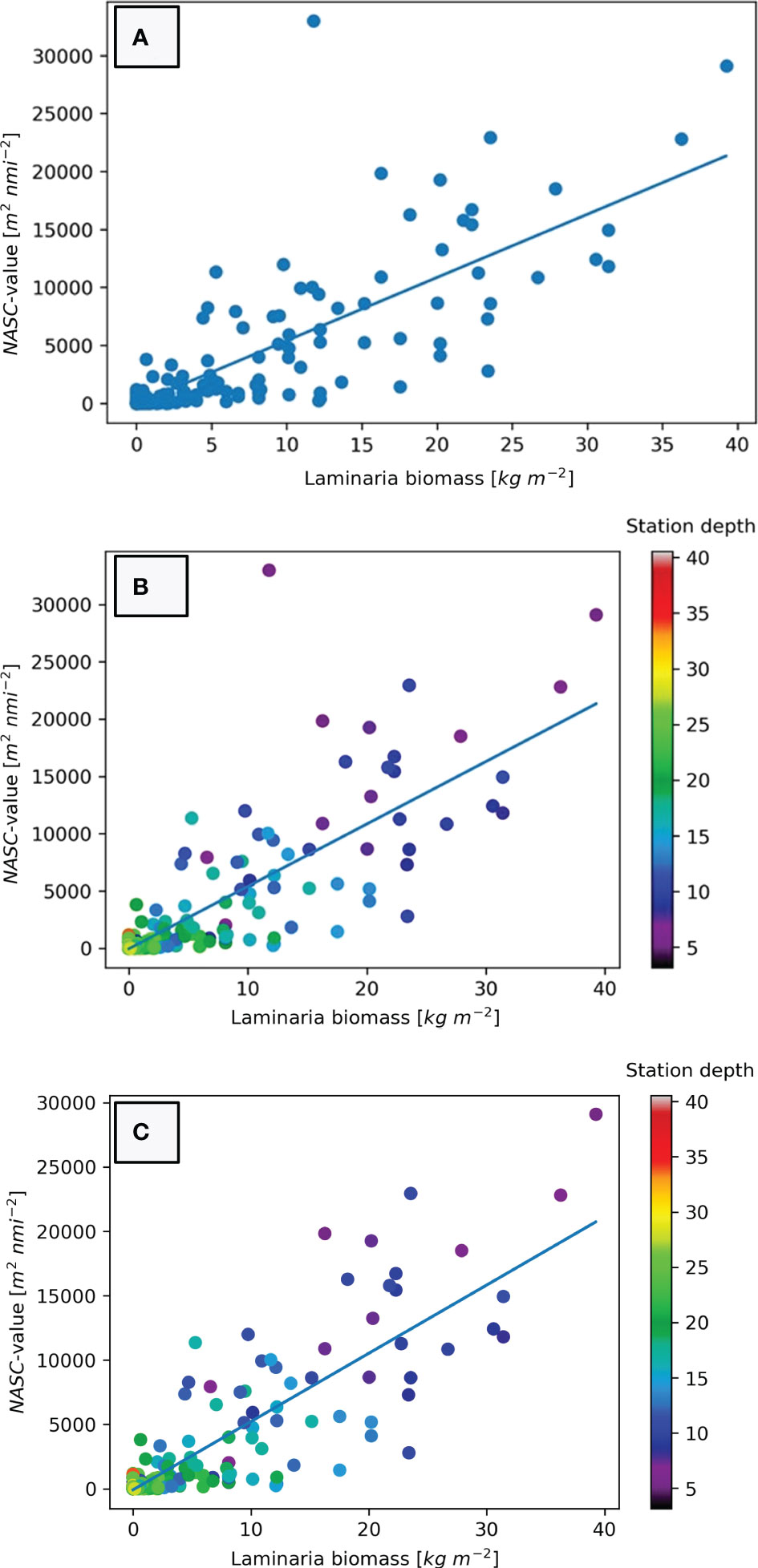
Figure 7 (A) Estimated biomass of kelp for each station (x-axis) plotted against NASC-value derived from echograms of the same stations (y-axis). A linear regression model has been established using least squares fit. (B) Cross-plot of estimated biomass and NASC-values from echograms with station depth indicated by a colour scale. Note the high density of points in the lower left corner of the figure. (C) Cross-plot of estimated biomass and NASC-values with colour coded depth scale where Helgeland station 113 has been removed from the dataset due to incompatibility between video and acoustic analysis.

$\begin{array}{ll}{\rho }_{kelp, predicted}=0.00184\times NASC+0.08014,R^2=0.6727& \text{(Eq. 1)}\end{array}$

In Figure 8 the depths of the investigated stations are plotted against the estimated biomass (a) and the echo amount (b). The figure demonstrates that many stations contain very little biomass, independent of depth. The stations with the highest biomass estimations are those with a depth of between 5 and 15 meters. Also, on deeper stations (especially those below 23 meters depth) the biomass estimate drops close to zero for all stations. These same trends can be seen when depth is plotted against NASC-value.

FIGURE 8

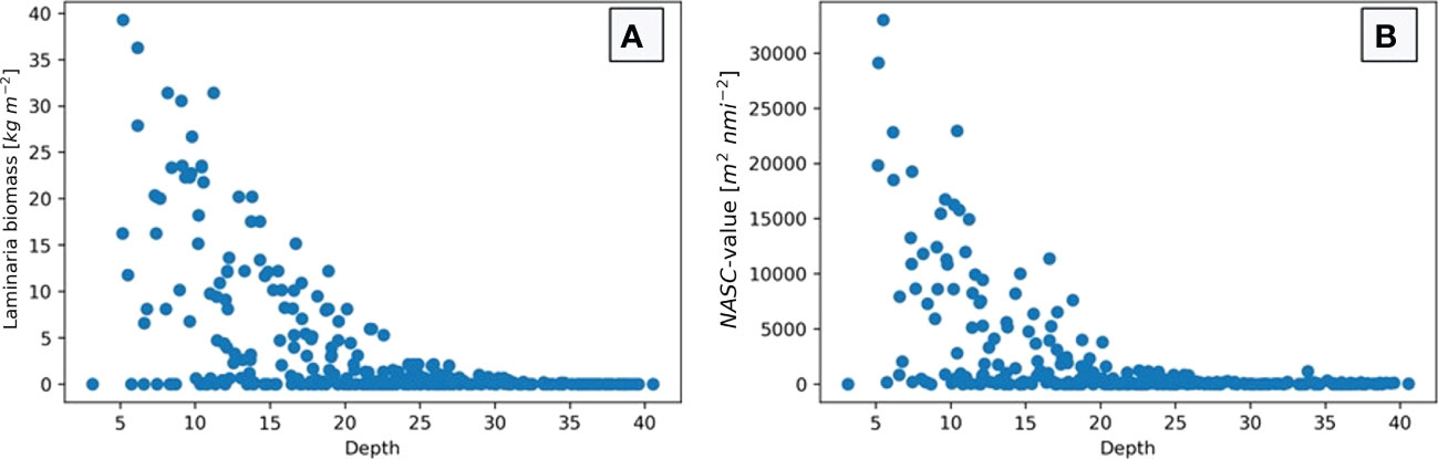
Figure 8 Biomass density estimate (A) and NASC-value (B) plotted with depth of each of the 298 stations in this study. The figures show a general decrease in biomass and backscatter strength as water depth increase, specifically for depths deeper than 20-25 meters when both estimates drop close to zero.

To further delineate the effect of water depth in our regression model we have added a colour coding of the station depth of each data point (Figure 7B). This shows that the stations with the highest deviation from the regression model are the shallow stations in our study. Furthermore, the relationship between the cross plots and station depth demonstrates that the deepest stations bare the lowest NASC-values. The low R²-value in Equation 1 is to a large degree caused by the outlier with the highest NASC-value in the study (Helgeland station 113). If we remove this outlier due to incompatibility between video and acoustic analysis, our new regression model (Figure 7C) can be expressed as:

$\begin{array}{ll}{\rho }_{kelp, predicted}=0.00189\times NASC+0.08231,R^2=0.7425& \text{(Eq. 2)}\end{array}$

This is a significant improvement of the statistical variation in the model and is likely a more reliable result.

Overall we found that echogram interpretation is on average 3-4 times less time consuming than biomass estimation from video sample analysis. Furthermore, acquisition of acoustic data was less dependent on stable weather- and water conditions and can also be done quicker than the video sampling, especially in deeper waters. The time it took to make the biomass calculation from video took on average around 14 minutes for each station, while echogram interpretation took around 4 minutes. However, the time for video analysis was variable, with rapid assessments (< 1 minute) for shallow stations with clear waters and a flat sandy seafloor and no kelp and over 20 minutes for deeper station with low visibility, structurally complex rocky seabed and dense kelp. The only drawback for interpretation of the acoustic data was that rough weather conditions could corrupt the data on shallow stations.

Discussion

Our study demonstrates that echosounder data can provide a reliable measure of kelp biomass, and are more efficient to collect and process than the standard method of video observations. There is great potential that such acoustic mapping of kelp forests could provide an efficient and practical method of evaluating the biomass density in a given area, which is useful for kelp researchers, harvesters and managers. However, unlike video and photograph surveys, echosounder data gives no information on species composition of epiphytes, sea urchin observations and other species in the kelp forest. The more detailed information on the benthic community and seabed substrate provided by the video samples has great value for additional studies that are not limited to biomass estimation but has a much higher time cost. Both methods are sensitive to weather conditions as they are operated from small boats in very shallow areas. The presented model that correlates the NASC-value and kelp biomass density shows a linear relationship with a reasonably good fit. It is assumed that the accuracy of model will continue to improve as data from future surveys are added to the datasets. We expect that echosounder data will provide valuable input to species distribution models in the future as they provide robust biomass estimations that can be acquired over vast areas in a cost-effective manner.

One of the major factors affecting the efficiency of the echogram interpretation was the performance of the bottom detection algorithm. When working correctly the algorithm minimized the need for manual interpretation, as the integration lines could be set based on the detected seabed. Although the algorithm performed well in most areas, it had issues in shallow waters, especially in depths less than five meters. This could be due to two reasons: 1) the presence of shallow air bubbles which caused the interpreted seabed to fluctuate between the actual seabed and the transducer near field (Figure 9A). 2) the algorithm seek a deep bottom which caused the seabed interpretation to fluctuate between the actual seabed and the 2^nd echo (Figure 9B). The latter could be avoided by changing the target depth for each station, but this was not done due to time constraints during the survey. Where any of these two difficulties were faced, the seabed has been manually interpreted, and the lower integration line is set 0,2 meters above this depth to minimize the risk of integrating the seabed and thus causing positively biased NASC-values. This manual interpretation is much more time consuming than setting the integration lines based on the bottom detection algorithm, but still a lot less time demanding than the analysis of video samples.

FIGURE 9

Figure 9 (A) Echogram from Helgeland station 132, one of the stations that has been excluded from the dataset. The shallow depth to the seabed and the large amount of air bubbles from the propeller makes it impossible to determine kelp canopy height. The average backscatter strength of the echogram is also remarkably high due to the bubble attenuation. (B) Echogram from Helgeland station 21 where the first half of the recordings are significantly influenced by the presence of air bubbles in the water column. Only the second half of the pings were used for calculating backscatter strength.

The upper integration line was set by visual inspection of the echograms at a distance above the visible kelp forest. This distance was not fixed but dependent on the individual echogram. I.e., if there was an abundance of shallow air bubbles in the echogram the integration line would be set as close to the kelp canopies as possible in order to exclude backscatter from bubble attenuation in the NASC-calculation. On the other hand, if there was no background noise in the water column, the integration line would be set at a reasonable distance above the canopies in order to include all kelp backscatter in the NASC-estimate. The air bubble correction module in the KORONA software failed to suppress the large air bubble clouds one some stations. The presence of these shallow bubbles represents one of the major weaknesses of computing an accurate and robust NASC-value. This was expected as weather conditions were very challenging during some field days and because frequent use of the propellers was necessary in the shallow areas the vessel operated in. Despite the challenges caused by air bubbles, the echograms appeared a lot cleaner and easier to interpret after the pre-processing.

In ideal conditions the NASC-value should be identical for one ping and 100 pings, but this is seldom the case, as seen in Figure 10, due to change in noise and signal attenuation through time. It proved difficult to identify and remove backscatter caused by unwanted artifacts due to that the heterogeneous acoustic signature of the kelp forests masked such artifacts extremely well. There were no practical ways to confidently distinguish undesirable reflections from inside the kelp forest because of the strong backscatter signal caused by the kelp canopies and undergrowth. Such “hidden” reflections would thus contribute to an artificially high NASC-value. To minimize the contribution to the backscatter strength caused by fish or other marine life that occasionally may swim beneath the transducer we decided to export as many pings as possible from each echogram to the database and then average the NASC-value. Another approach to this problem would be to manually inspect the echograms and select the 100-pings bin with the least amount of noise both from inside the kelp forest and in the water column. However, this approach would bring an element of subjectiveness to the method that could be a drawback for developing a standardised methodology for kelp mapping.

FIGURE 10

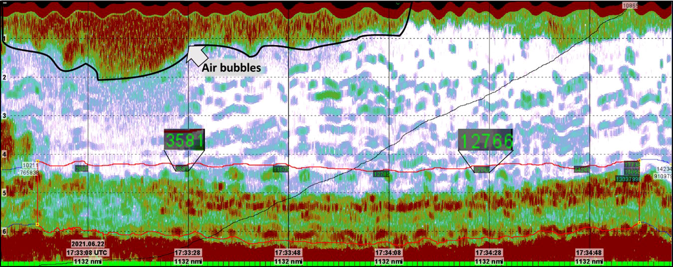
Figure 10 Echogram from Helgeland station 174. Notice the vast difference in estimated NASC-value due to the presence of air bubbles in the upper water column.

Although the 120 kHz echograms were much cleaner than the 32kHz, these data were not unaffected by unwanted “noise” in the water column and close to the seabed. The signal-to-noise ratio is dependent on a number of factors including wave- and current activity, water depth, the use of propeller on the vessel, bottom depth, frequency and instrument-generated noise (Korneliussen, 2000). In this shallow water setting, the primary factor for suppressing the backscatter from the kelp was the presence of air bubbles near the sea surface. These air bubbles attenuated the acoustic signal causing the echo integration results to be negatively biased (Dalen and Lovik, 1981). This effect can be seen on Figure 10 where the NASC for a single station varies with a factor of 3.5 due to the presence of air bubbles in the uppermost water column. One way to tackle this problem is to scrutinize the amount of backscatter in each bin and remove bins with extreme NASC-values. This was not done in this study because of the aim to establish a general and robust methodology. Instead, each station was acoustically monitored for approximately 2 minutes, corresponding to around 1200 pings and 12 100-ping bins. Thus, by averaging the NASC-values over all bins a robust NASC-estimate has been established. Furthermore, the spike- and the noise filtering added in the processing of the data adds smoothing to the data. This minimizes the effects of abnormal NASC-values due to erroneous pings or noise.

When working in such shallow-water conditions, there is also a threat that the air bubbles from the propeller penetrate the kelp canopy and interfere with the backscatter strength of the kelp. This was a major issue in this study, especially when the ship was using astern propulsion to fight current or wind, which would cause the air bubbles to pass through the transducer beam. This made it near impossible to determine the height of the canopies and, furthermore, would result in a significantly overestimated NASC-estimate. This can be seen in Figure 9A. Stations where the entire echogram was influenced by air bubbles from the thruster was excluded from the dataset. At stations where only some of the echogram was affected by this unwanted noise, the distorted parts was excluded from interpretation, while the unaffected parts were kept for further scrutinizing (Figure 9B). The decision to exclude parts of the echogram were always made by two interpreters in order to ensure consistency and that only indisputably corrupt data were excluded.

The modelled relationship between echo amount and kelp biomass (Figure 7A & Equation 1) is evidently too simplistic to fully explain the kelp distribution in all areas and has poor prediction power in areas with no vegetation. This is demonstrated by the relatively low R²-value of 0.673. However, this somewhat low level of determination is largely due to the deviation of Helgeland station 113 that can be seen as an obvious outlier in Figures 7A, B. This station had the highest NASC-value in the study (31985 m² nmi^-2), but a modest biomass density of 11.785 kg m^-2. This station has been scrutinized in order to understand the distinct deviation from the model: Helgeland station 113 is situated on a rocky and rugged sloping seabed with a water depth of merely 4.5 meters. The area was densely covered by kelp, and from the video analysis we have found the height of the kelp to be approximately 1 meter, but we could also see higher vegetation in the vicinity of the station. As previously mentioned, the horizontal distance between the location of the drop-camera and the hull-mounted transducer may be as much as 6 meters depending on current and movement. We believe that this offset is the main cause for the mismatch between acoustic amount and biomass estimate. At this station it is likely that the transducer was located over a patch of vegetation that was both denser and higher than what the drop-camera was. This was partially confirmed by visual inspection of the echogram from the station which showed a vegetation height of more than 1.5 meters. Due to the uncertainty regarding the comparability of the two datasets at this station, we chose to discard it from our final model, as presented in Figure 7C and Equation 2. The resulting linear model is still not able to predict areas without any kelp at all, but for practical use this flaw is regarded to be negligible. Although the model has a reasonably good fit (R^{2 =} 0.7425), it is not able to accurately predict the biomass density estimates of specific stations. For our dataset it can be seen from that NASC-values of approximately 12 000 m² nmi^-2 includes biomass density estimates ranging from 5.3 kg m^-2 (NASC=11359 m² nmi^-2) to 31.4 kg m^-2 (NASC=11807 m² nmi^-2) (Figure 7C). Despite this variability we believe that the linear model will provide a vital input to spatial distribution models as a cost-effective indicator of standing kelp biomass in large areas.

Further work

There are several improvements to this method that could increase data quality and interpretation accuracy. To limit the background- and transient noise, the acquisition design should be improved. The transducers that are now mounted on the hull of the ship could be moved to the keel in order to avoid attenuation and backscatter from air bubbles present in shallow water. This will be done before further stations are sampled. To further improve the model a larger database is needed. It is believed that the model will continue to improve as more stations are surveyed the coming years and that both the statistical variance and our understanding of the acoustic response will progress as more data points are added. With more data points it will also be possible to perform a thorough statistical analysis and thereby identify and scrutinize outliers. To be able to analyse the comparability of the video samples and the acoustic data in a consistent way, a tool for extracting the acoustic height of the kelp forest should be developed. This will make it possible to compare the estimated density and heights of the kelps for each station. We will suggest this to the developers of the interpretation software. The proposed model can be implemented in statistical species distribution models, which now are drawn e.g. from detailed topographic- and substrate maps coupled with observations of wave exposure and bottom current speed (Filbee-Dexter et al., 2018; van Son et al., 2020; Gundersen et al., 2021). These models can be particularly useful in vast areas or other areas where sufficient sampling is difficult but acquiring high-resolution covariance grids represents a major challenge. It is believed that biomass estimations from acoustics will further improve the accuracy of such models. The proposed methodology should be further developed to also include acoustic transects. This is needed to cover vast areas in a feasible and efficient way. It is believed that this is key to provide extensive and robust distribution models for this highly productive marine habitat. Acoustic transects will be acquired in future surveys.

Conclusions

In this study we have demonstrated how acoustics can be used to measure kelp biomass. We provide a regression model relating the nautical area backscatter coefficient derived from echograms to biomass of kelp. This model shows a robust relationship between the two variables. We show that the proposed method is efficient and is suitable for performing large (kilometer) scale quantifications of kelp biomass and applicable to assessments and monitoring worldwide. Quantifying the spatial distribution of kelp can fill in critical gaps of knowledge in the understanding of the climate role of blue carbon (Krause-Jensen et al., 2018) and for monitoring purposes of human exploitation of kelp resources including kelp harvesting (Gouraguine et al., 2021).

Data availability statement

The raw data supporting the conclusions of this article will be made available by the authors, without undue reservation.

Author contributions

HS planned the fieldwork with KN, conducted the fieldwork with LC and did biomass estimations. KK led the writing with contributions from all co-authors and conducted the acoustic interpretation with LC. KK and HS collected and produced all figures. KF structured the ms and did proofreading. All authors contributed to the article and approved the submitted version.

Funding

The research was financed by the Ministry of Trade, Industry and Fisheries through grant 14914 - Blue forest research.

Conflict of interest

The authors declare that the research was conducted in the absence of any commercial or financial relationships that could be construed as a potential conflict of interest.

Publisher’s note

All claims expressed in this article are solely those of the authors and do not necessarily represent those of their affiliated organizations, or those of the publisher, the editors and the reviewers. Any product that may be evaluated in this article, or claim that may be made by its manufacturer, is not guaranteed or endorsed by the publisher.

References

Assis J., Serrão E. A., Duarte C. M., Fragkopoulou E., Krause-Jensen D. (2022). Major expansion of marine forests in a warmer Arctic. Front. Mar. Sci. 9. doi: 10.3389/fmars.2022.850368

PubMed Abstract | CrossRef Full Text | Google Scholar

Bennion M., Fisher J., Yesson C., Brodie J. (2019). Remote sensing of kelp (Laminariales, ochrophyta): Monitoring tools and implications for wild harvesting. Rev. Fish. Sci. Aquac. 27 (2), 127–141. doi: 10.1080/23308249.2018.1509056

CrossRef Full Text | Google Scholar

Blight A., Foster-Smith R., Sotheran I., Egerton J., McAllen R., Savidge G. (2011). Development of a methodology for the quantitative assessment of ireland’s inshore kelp resource. Mar. Inst. Avaialble at: http://hdl.handle.net/10793/702.

Google Scholar

Cavanaugh K. C., Cavanaugh K. C., Bell T. W., Hockridge E. G. (2021). An automated method for mapping giant kelp canopy dynamics from UAV. Front. Environ. Sci. 8. doi: 10.3389/fenvs.2020.587354

CrossRef Full Text | Google Scholar

Dalen J., Lovik A. (1981). The influence of wind-induced bubbles on echo integration surveys. J. Acoust. Soc. America 69 (6), 1653–1659. doi: 10.1121/1.385943

CrossRef Full Text | Google Scholar

Duarte C. M., Gattuso J.-P., Hancke K., Gundersen H., Filbee-Dexter K., Pedersen M. F., et al. (2022). Global estimates of the extent and production of macroalgal forests. Global Ecol. Biogeogr. 31 (7), 1422–1439. doi: 10.1111/geb.13515

CrossRef Full Text | Google Scholar

Duffy J. E., Benedetti-Cecchi L., Trinanes J., Muller-Karger F. E., Ambo-Rappe R., Boström C., et al. (2019). Toward a coordinated global observing system for seagrasses and marine macroalgae. Front. Mar. Sci. 6, 317. doi: 10.3389/fmars.2019.00317

CrossRef Full Text | Google Scholar

Filbee-Dexter K., Wernberg T. (2020). Substantial blue carbon in overlooked Australian kelp forests. Sci. Rep. 10 (1), 1. doi: 10.1038/s41598-020-69258-7

PubMed Abstract | CrossRef Full Text | Google Scholar

Filbee-Dexter K., Wernberg T., Norderhaug K. M., Ramirez-Llodra E., Pedersen M. F. (2018). Movement of pulsed resource subsidies from kelp forests to deep fjords. Oecologia. 187(1):291–304. doi: 10.1007/s00442-018-4121-7

PubMed Abstract | CrossRef Full Text | Google Scholar

Foote K. G. (1987). Calibration of acoustic instruments for density estimation: A practical guide. Int.Counc.Explor.Sea.Coop.Res.Rep 144, 57.

Google Scholar

Gouraguine A., Moore P., Burrows M., Vinasco E., Ariz L., figueroa fabrega L., et al. (2021). The intensity of kelp harvesting shapes the population structure of the foundation species lessonia trabeculata along the Chilean coastline. Mar. Biol. 168. doi: 10.1007/s00227-021-03870-7

CrossRef Full Text | Google Scholar

Gundersen H., Rinde E., Bekkby T., Hancke K., Gitmark J. K., Christie H. (2021). Variation in population structure and standing stocks of kelp along multiple environmental gradients and implications for ecosystem services. Front. Mar. Sci. 8. doi: 10.3389/fmars.2021.578629

CrossRef Full Text | Google Scholar

Kjerstad N., Woll A., Fosså J. H., Sevaldsen E. (1995). Mengdeberegning av stortare (Laminaria hyperborea) ved hjelp av ekkointegrator (Å9420).

Google Scholar

Korneliussen R. (2000). Measurement and removal of echo integration noise. ICES J. Mar. Sci. 57 (4), 1204–1217. doi: 10.1006/jmsc.2000.0806

CrossRef Full Text | Google Scholar

Krause-Jensen D., Lavery P., Serrano O., Marbà N., Masque P., Duarte C. M. (2018). Sequestration of macroalgal carbon: The elephant in the blue carbon room. Biol. Lett. 14 (6), 20180236. doi: 10.1098/rsbl.2018.0236

PubMed Abstract | CrossRef Full Text | Google Scholar

MacLennan D. (2002). A consistent approach to definitions and symbols in fisheries acoustics. ICES J. Mar. Sci. 59 (2), 365–369. doi: 10.1006/jmsc.2001.1158

CrossRef Full Text | Google Scholar

MacLennan D., Simmonds E. J. (2005). Fisheries acoustics. 2nd ed (Chapman & Hall) 20–126. doi: 10.1002/9780470995303.ch2

CrossRef Full Text | Google Scholar

Minami K., Tojo N., Yasuma H., Ito Y., Nobetsu T., Fukui S., et al. (2014). Quantitative mapping of kelp forests (Laminaria spp.) before and after harvest in coastal waters of the shiretoko peninsula, Hokkaido, Japan. Fish. Sci. 80 (3), 405–413. doi: 10.1007/s12562-014-0731-0

CrossRef Full Text | Google Scholar

Mora-Soto A., Palacios M., Macaya E. C., Gómez I., Huovinen P., Pérez-Matus A., et al. (2020). A high-resolution global map of giant kelp (Macrocystis pyrifera) forests and intertidal green algae (Ulvophyceae) with sentinel-2 imagery. Remote Sens. 12 (4), 4. doi: 10.3390/rs12040694

CrossRef Full Text | Google Scholar

Norderhaug K. M., Brandt C. F., Espeland S. H., Albretsen J., Christensen-Dalsgaard S., Ohldieck M. J., et al. (2021). Sustainable kelp harvesting–assesment of sustainability criteria for vikna, Norway (IMR). Available at: https://www.hi.no/templates/reporteditor/report-pdf?id=49308&05873304.

Google Scholar

Norderhaug K. M., Christie H., Fosså J. H., Fredriksen S. (2005). Fish–macrofauna interactions in a kelp ( laminaria hyperborea ) forest. J. Mar. Biol. Assoc. United Kingdom 85 (5), 1279–1286. doi: 10.1017/S0025315405012439

CrossRef Full Text | Google Scholar

Norderhaug K., Filbee-Dexter K., Freitas C., Birkely S., Christensen L., Mellerud I., et al. (2020a). Ecosystem-level effects of large-scale disturbance in kelp forests. Mar. Ecol. Prog. Ser. 656, 163–180. doi: 10.3354/meps13426

CrossRef Full Text | Google Scholar

Norderhaug K. M., Nedreaas K., Huserbråten M., Moland E. (2020b). Depletion of coastal predatory fish sub-stocks coincided with the largest sea urchin grazing event observed in the NE Atlantic. Ambio 50:163–73. doi: 10.1007/s13280-020-01362-4

PubMed Abstract | CrossRef Full Text | Google Scholar

Ona E. (1999). Methodology for target strength measurements (With special reference to in situ techniques for fish and mikro-nekton). doi: 10.17895/ICES.PUB.5367

CrossRef Full Text | Google Scholar

Pessarrodona A., Assis J., Filbee-Dexter K., Burrows M. T., Gattuso J.-P., Duarte C. M., et al. (2022). Global seaweed productivity. Sci. Adv. 8 (37), eabn2465. doi: 10.1126/sciadv.abn2465

PubMed Abstract | CrossRef Full Text | Google Scholar

Pessarrodona A., Foggo A., Smale D. A. (2018). Can ecosystem functioning be maintained despite climate-driven shifts in species composition? insights from novel marine forests. J. Ecol. 107 (1), 91–104. doi: 10.1111/1365-2745.13053

CrossRef Full Text | Google Scholar

Pörtner H.-O., Roberts D. C., Adams H., Adler C., Aldunce P., Ali E., et al. (2022). Climate change 2022: Impacts, adaptation and vulnerability. IPCC Sixth Assessment Report.

Google Scholar

Shao H., Minami K., Shirakawa H., Kawauchi Y., Matsukura R., Tomiyasu M., et al. (2019). Target strength of a common kelp species, saccharina japonica, measured using a quantitative echosounder in an indoor seawater tank. Fish. Res. 214, 110–116. doi: 10.1016/j.fishres.2019.01.009

CrossRef Full Text | Google Scholar

Shao H., Minami K., Shirakawa H., Maeda T., Ohmura T., Fujikawa Y., et al. (2017). Verification of echosounder measurements of thickness and spatial distribution of kelp forests. J. Mar. Sci. Technol. 25 (3), 10. doi: 10.6119/JMST-016-1229-1

CrossRef Full Text | Google Scholar

Steen H. (2020). Assessment of kelp harvesting fields in Møre og Romsdal and Trøndelag in 2020. Rapport fra Havforskningen Nr. 31-2020.

Google Scholar

Steen H., Moy F. E., Bodvin T., Husa V. (2016). Regrowth after kelp harvesting in nord-trøndelag, Norway. ICES J. Mar. Sci.: J. Du Conseil 73 (10), 2708–2720. doi: 10.1093/icesjms/fsw130

CrossRef Full Text | Google Scholar

St-Pierre A. P., Gagnon P. (2020). Kelp-bed dynamics across scales: Enhancing mapping capability with remote sensing and GIS. J. Exp. Mar. Biol. Ecol. 522, 151246. doi: 10.1016/j.jembe.2019.151246

CrossRef Full Text | Google Scholar

van Son T. C., Nikolioudakis N., Steen H., Albretsen J., Furevik B. R., Elvenes S., et al. (2020). Achieving reliable estimates of the spatial distribution of kelp biomass. Front. Mar. Sci. 7. doi: 10.3389/fmars.2020.00107

CrossRef Full Text | Google Scholar

Wernberg T., Bennett S., Babcock R. C., de Bettignies T., Cure K., Depczynski M., et al. (2016). Climate-driven regime shift of a temperate marine ecosystem. Science 353 (6295), 169–172. doi: 10.1126/science.aad8745

PubMed Abstract | CrossRef Full Text | Google Scholar

Wernberg T., Krumhansl K., Filbee-Dexter K., Pedersen M. F. (2019). “Chapter 3 - Status and Trends for the World’s Kelp Forests," in World Seas: An Environmental Evaluation (Second Edition). Ed. Sheppard C. (Academic Press), 57–78. doi: 10.1016/B978-0-12-805052-1.00003-6

CrossRef Full Text | Google Scholar

Woll A., Kjerstad N., Fosså J. H., Dyb J.e. (1999). Utvikling av en akustisk metodikk for ressurskartlegging av stortare (Laminaria hyperborea) (Å9916).

Google Scholar

Young M., Ierodiaconou D., Womersley T. (2015). Forests of the sea: Predictive habitat modelling to assess the abundance of canopy forming kelp forests on temperate reefs. Remote Sens. Environ. 170, 178–187. doi: 10.1016/j.rse.2015.09.020

CrossRef Full Text | Google Scholar