 Elisa Halewood
 Keri Opalk
 Lillian Custals2
 Dennis A. Hansell
 Craig A. Carlson
- 1Marine Science Institute, Department of Ecology, Evolution and Marine Biology, University of California Santa Barbara, Santa Barbara, CA, United States
- 2Department of Ocean Sciences, Rosenstiel School of Marine and Atmospheric Science, University of Miami, Miami, FL, United States
This document describes best practices for analysis of dissolved organic matter (dissolved organic carbon and total dissolved nitrogen) in seawater samples. Included are SOPs for sample collection and storage, details for laboratory analysis using high temperature combustion analysis on Shimadzu TOC analyzers, and suggestions for best practices in quality control and quality assurance. Although written specifically for GO-SHIP oceanographic community practices, many aspects of sample collection and processing are relevant to DOM determination across oceanic regimes and this document aims to provide updated methodology to the wider marine community.
1 Introduction
Dissolved organic matter (DOM), operationally defined as organic matter that passes through a submicron filter, is a complex mixture of organic molecules comprised of carbon, hydrogen and oxygen as well as nitrogen, phosphorus and sulfur. Resolving the dynamics of each DOM fraction helps to elucidate the greater questions of DOM biogeochemical cycling. At ~662 ± 32 Pg (1015 g) C, oceanic dissolved organic carbon (DOC) is one of the largest bioreactive pools of carbon in the ocean (Williams and Druffel, 1987; Hansell and Carlson, 1998; Hansell et al., 2009), and is comparable to the mass of inorganic C in the atmosphere (MacKenzie, 1981; Eppley et al., 1987; Fasham et al., 2001). Perturbations in the sources or sinks of the oceanic DOC pool impact the balance between oceanic and atmospheric CO2, perhaps making it climatically significant (Ridgwell and Arndt, 2014). In addition, most of the standing stock of fixed nitrogen in the surface ocean (<200 m) is in the form of dissolved organic nitrogen (DON) (Bronk, 2002; Aluwihare and Meador, 2008; Letscher et al., 2013). As such, it is important to understand the processes that control DOC and DON distribution, inventories and fluxes in the global ocean.
Prior to the 2000’s, there was a lack of high-quality data to adequately describe and quantify DOM in the ocean. In the 1980’s, controversy over methods of DOC and total dissolved nitrogen (TDN) analyses in seawater (Williams and Druffel, 1988) resulted in efforts by the marine geochemistry community to improve accuracy of the measurement and establish inter-comparability of data sets (Sharp, 1993; Sharp et al., 1995; Sharp et al., 2002a; Sharp et al., 2002b), proper blank procedures (Benner and Strom, 1993) and methods using reference materials (Hansell, 2005). The High Temperature Combustion (HTC) method using commercial instruments such as the Shimadzu Total Organic Carbon (TOC) Analyzer are now common for measuring DOC and TDN in seawater. Advances in analytical skill and increased frequency of global ocean sampling (through time-series sites and in conjunction with basin scale programs such as the U.S. Global Ocean Ship-Based Hydrographic Investigation Program (U.S. GO-SHIP)) have greatly improved temporal and spatial resolution of DOC variability (Hansell et al., 2009; Carlson et al., 2010; Hansell et al., 2021). Further, DOM’s contributions to the ecology and biogeochemistry of the ocean’s water column have been illuminated (Baetge et al., 2021; Liu et al., 2022).
This paper describes procedures for collection and measurement of DOC and TDN (the latter used in conjunction with measurements of nitrate, nitrite, and ammonia to derive DON concentration) in discrete seawater samples. It is suitable for the assay of oceanic levels of DOC (typically<80 µmol C kg-1) and total dissolved nitrogen (<40 µmol N kg-1). It presents best practices for achieving improved determination using the HTC method following the approach of Carlson et al. (2010), which has been used on U.S. GO-SHIP cruises since 2003. The basic approach remains the same but the analyzers have been optimized over the years. The instruments discussed and procedures described are those specific to the methods employed in the Hansell Lab at the University of Miami’s Rosenstiel School of Marine and Atmospheric Science and the Carlson Lab at the University of California Santa Barbara. This document builds upon existing guidelines for analysis of DOC in seawater (Tappin and Nimmo, 2019), and seeks to provide detailed updates and step by step protocols on sample collection & storage, optimizing Shimadzu TOC systems for high throughput of seawater samples, and quality assessment/quality control (QA/QC) practices using calibration and reference materials. In addition, we present methodological procedures for coupled TDN analysis using Shimadzu TOC systems. We have chosen to highlight Shimadzu Scientific Instruments because of ease of use of their off-the-shelf TOC instruments and their excellent limit of detection, but instruments from other manufacturers with equivalent detection capabilities or custom-built machines may also be appropriate. A previous version of this manuscript (Halewood et al., 2022) was published as part of the GO-SHIP Repeat Hydrography Practices Collection. This version is applicable to a wider marine audience.
2 Sample collection and storage
Proper sampling techniques and handling are essential to provide high quality data. Open ocean waters contain relatively low concentrations of DOC (~35-80 µmol C kg-1, Hansell et al., 2009) compared to dissolved inorganic carbon (DIC) (~1900-2200 µmol kg-1) and are easily contaminated via poor handling, inadequately cleaned apparatus, inadvertent atmospheric exposure to volatile contaminants, or improper storage conditions. The methods described here aim to minimize these sources of error.
2.1 Sample bottles
It is recommended that samples be filtered directly from the collection bottle (i.e., Niskin bottle) through an in-line filter (see below) and into a pre-cleaned sample bottle. To minimize handling, we recommend pre-combusted 40 mL glass vials that fit the Shimadzu TOC auto-sampler. These vials are made of chemically inert Type I borosilicate glass. While these can be purchased certified clean (meeting the requirements of the US Environmental Protection Agency (EPA) for the testing of potentially harmful environmental contaminants in water or soil samples and TOC analysis) we have found these not sufficiently clean for low concentration oceanic DOC measurements. We prepare vials in house as below to be clean and free of substances that might influence analysis. If glass is logistically challenging, samples can also be collected into acid washed high-density polyethylene (HDPE) or polycarbonate (PC) bottles. Tests have shown that DOC concentration measured from glass, PC and HDPE bottles are comparable at the µmol L-1 resolution (Supplementary Appendix A). Both glass and plastic sample containers are re-usable after proper cleaning. Prior to first use, or between uses, HDPE or PC bottles should be soaked in 1 M hydrochloric acid (HCl Certified ACS Plus grade, see Appendix B), rinsed with low TOC water (UV -Nanopure™ or UV- MilliQ® generated and hereafter referred to as “ultrapure water/UW”), and air dried completely before capping. Glass vials are easiest to prepare and ensure that they are clean. These are emptied, rinsed 3x with UW, dried and heated at 450°C for ≥ 4 hours to remove organics (manufacturer’s maximum recommended working temperature for this type of borosilicate glass is 500°C.) The use of Polytetrafluoroethylene
(PTFE) lined silicone septa or cap is recommended for the glass vials, and it is recommended that those be soaked in 1 M HCl, rinsed with ultrapure water and dried between uses. See supplementary material for detailed cleaning procedures (SOP1) and suggested equipment (Appendix B).
2.2 Filters
DOM is operationally defined as the fraction of total organic matter passing through a submicron filter (i.e., 0.22 - 0.7 μm). In practice, oceanographers commonly use Whatman® GF/F filters (nominal pore size 0.7 μm) as the cutoff between particulate and dissolved organic matter fractions (Knap et al., 1996). These borosilicate glass fiber filters are most commonly used for bulk measures of DOC and TDN (Carlson et al., 1998) as they can be easily prepared by pre-combustion and the flow rate through the filters is ideal for rapid in-line sampling. GF-75 filters (0.3 μm nominal pore size, Advantec MFS, USA) are also appropriate as they can be combusted, and may be preferred when concurrently measuring subfractions of DOM (such as amino acids) where maximum particle exclusion from the dissolved pool is desired. For bulk dissolved organic matter concentrations, we do not resolve differences between GF-75 and GF/F use. The GF-75 and/or GF/F filters are prepared by combusting at 450°C for 4 hours in foil packets. We do not exceed 450°C because the filter matrix may become altered at higher temperatures. After the filter packets are cooled, the foil pack containing filters is sealed into secondary plastic bags until use. It is advised to pack only enough filters needed for a single cast in each foil packet to avoid long exposure of combusted filters to airborne volatile organic contaminants. In preparation for sampling, a filter is placed into a pre-cleaned 47 mm polycarbonate filter cartridge. Gravity filtration is always recommended to avoid cell rupture and tearing of filters. Refer to supplementary SOP1 and SOP2 for details on filter preparation and in-line cartridge cleaning, and Appendix B for relevant product information.
2.3 Niskin sampling procedure
It is important to select a DOM-clean workspace in the shipboard laboratory (i.e., well ventilated and free of volatile organics, organic fixatives, fresh paint, permanent markers, smoke, etc.) and to maintain this area in a clean fashion for storing, cleaning and preparing sampling gear on a daily basis. Cover the bench top with absorbent liner and replace frequently. The sampling equipment (e.g., filter holders, silicone tubing) should be cleaned in a dilute acid solution (1 M HCl) prior to each use (Supplementary SOP1). It is recommended that pre-printed labels be used; alternatively, labeling with markers should only be done when vials are tightly sealed as permanent markers contain solvent that may contaminate samples.
Gloves should be worn during DOM collection and handling to minimize contamination. Powder-free nitrile, polyethylene and latex-free vinyl gloves are safe options as they have low organic leaching when exposed to seawater. Because DOM samples can be easily contaminated, it is recommended that collection from the CTD rosette occur as soon as possible after gas sampling. It is also recommended that anyone sampling from the rosette prior to collection of DOM samples wear gloves. If that is not possible, every effort must be made not to touch the Niskin bottle’s spigot (i.e., the path of the water stream, from Niskin to sample bottle, must be kept very clean). Most importantly, any sampling preceding DOM must avoid use of grease or Tygon® tubing as these are known to contaminate DOM at the µmolar level. If Tygon® is unavoidable for other samplers, supplying a small silicone tubing section as an adapter between the Niskin and Tygon® is advised. Mechanical grease from ship operations (e.g., CTD wire lubricant) should never come in contact with the Niskin bottle’s sampling valve or spigot.
Whether or not a sample is filtered prior to analysis depends on the goal of the measurement. If DOC and TDN are the variables of interest, then all samples should be filtered. However, the handling of filters and apparatus can increase potential for contamination, so in some cases filtration can be bypassed (Mopper and Qian, 2006). In most oligotrophic waters or depths > 250 m away from ocean margins, DOC is the dominant component of TOC, exceeding the carbon inventory of organic particles by several orders of magnitude (Cauwet, 1978; Hansell et al., 2012). In high productivity areas, a substantial portion of organic carbon in the euphotic zone may be present in particulate form, and many of those particles may be large and heterogeneously distributed in a sample, such that these sample types should be filtered. Supplementary Appendix A (Figure A2) presents vertical profiles of TOC and DOC in contrasting regions as an example. As important components of global carbon cycles, accurate measurement of each fraction is critical for constraining mass balance of carbon in ocean models. For consistency when sampling in both oligotrophic and eutrophic environments, filtering is recommended, at a minimum, for all ≤ 250-m samples. In oligotrophic environments, one filter may be re-used for several consecutive samples around the rosette to conserve resources. It is recommended to filter samples from the greatest depth to the shallowest; particulate concentrations will typically increase nearer the surface ocean, which could cause the filter to clog or the particles to disrupt, requiring more filters to be used for one station. Studies have shown that DOC can sorb to active sites on GF/F filters, which raises the question whether filtration through GF/F strips organic matter from the DOC filtrate (Turnewitsch et al., 2007; Novak et al., 2018). Approximately 60 mL of sample are passed through a new filter during the flushing and vial rinsing procedure. Tests after the filter and bottle rinsing step show no further stripping of organic carbon from DOC filtrate can be resolved at the µmol kg-1 level (Supplementary Figure A3). These results suggest that sorption of dissolved organic matter to combusted GF/F filters saturates the active sites on a combusted filter rapidly (within ~ 60 mL) and is not a DOC stripping concern when filtering samples for bulk DOM analysis.
Samples should be gravity filtered at the rosette via an in-line filter cartridge housing a combusted GF/F filter and attached directly to the Niskin spigot via acid clean platinized silicone tubing (Cole-Parmer, Supplementary Appendix B). This type of platinum cured silicone tubing offers durability and minimizes organic leaching compared to Tygon®. Rinse the sample container and cap three times with sample water prior to filling it three quarters full (refer to Supplementary SOP2 for step-by-step instructions). It is important to collect sufficient volume for analysis and to minimize surface area to volume ratio of the container (a minimum of 15 mL in a glass vial or 30 mL in an HDPE bottle for each analyte desired, DOC or TDN) while also taking care to not overfill the sample container. It bears repeating that care should be taken during sampling to avoid any obvious contaminants such as cigarette smoke, paint fumes, excessive engine fumes in the sampling bay, or organic solvents in the laboratories, etc. Sampling equipment (combusted filters and glassware in particular) should be kept carefully sealed right up to the time of sampling to avoid sorption of airborne contaminants onto cleaned surfaces. Always log unusual events regarding the samples; add notes that may be useful for explaining results.
2.3.1 Example collection plan
For U.S. GO-SHIP sections, 24-36 Niskin bottles (24-36 depths over the entire water column) are sampled at alternating stations (i.e., station sampling for DOM occurs at ~60 nautical mile intervals). For other campaigns the sampling decisions with regard to horizontal or vertical resolution will depend on the scientific aims of the project. To assess sample handling error, it is recommended that replicate samples be collected randomly from a subset of depths over a hydrographic profile. For current U.S. GO-SHIP sections, the standard practice is to replicate 2 Niskin bottles per 36 bottle cast (~6% replication in sample set).
2.4 Sample preservation and storage
Many DOM analytical instruments are not stable enough to conduct at-sea analyses; thus, safe storage of samples is essential. After collection at the rosette, samples can be preserved and stored for later analysis in a shore-based laboratory using several methods.
2.4.1 Frozen storage
Seawater samples collected into glass should not be stored at temperatures below -20°C as colder temperatures (e.g.,< -40°C) can result in breakage of the glass upon thawing. If storing at temperatures< -20°C is the only option available then the use of plastic sampling containers (HDPE or PC) is a safe alternative for bulk DOC/TDN analyses. Frozen samples that have been acidified should only be stored in glass as plastic will leach upon long term exposure to acid. For samples collected in plastic and not acidified it is important to freeze as promptly as possible after collection to avoid changes in organic matter due to biological activity. Upon storing frozen samples, it is imperative that these samples not be overfilled as water will expand with freezing. Tests have shown that a salinity gradient is set up during freezing with high brine/high DOC water potentially being displaced through the cap threads if the bottle is overfilled (Supplementary Appendix, Figure A4). This extrusion results in a diluted DOM concentration, rendering the sample compromised. Care should be taken to freeze samples in an upright position, and check that caps are tightly sealed prior to freezing and storage and again before shipping. Segregate frozen samples from any other volatile organic material in storage to prevent airborne volatile organic contamination. Frozen samples can be safely stored for periods of years (see sample storage tests, Supplementary Appendix A). Prior to analysis, frozen samples must be completely thawed at room temperature and homogenized. Use of a mechanical device such as a vortex mixer is ideal. The mixer should be set to a high enough speed that a vortex is visible and extends from the surface of the sample through to the bottom of the container.
2.4.2 Acidified and liquid storage
Shipping of frozen samples is costly and often unreliable; thus, an alternative to frozen storage is collection in glass vials, acidification and storage in liquid form. Samples should be acidified soon after collection by adding 2 µl of 4 M hydrochloric acid (ACS or trace metal grade) per 1 mL of sample. This ratio of acid/sample should bring the sample to pH 2-3. Periodically check samples to ensure this low pH is reached. This can be done by drawing out a few mL of sample (using a non-sterile tip and DOC clean pipette) and using this volume to wet a pH strip. Never immerse a pH strip directly into a sample as this will result in contamination. At pH 2-3 biological activity is halted, ensuring safe storage, and inorganic carbon species are converted to CO2 and later degassed from the sample solution with sparging on the TOC system at the time of analysis (sparging at the time of sample collection is not recommended as less handling is best for preventing contamination). A repeater pipette with an acid-cleaned tip is recommended for acid addition (refer to Supplementary SOP2 for details). It is recommended to prepare a 100 – 500 mL batch of 4 M HCl using high purity acid (Certified ACS Plus, Supplementary Appendix B) diluted with ultrapure water and then aliquot and seal the 4 M HCl into 1-2 mL pre-combusted glass ampoules. It is advised that a new ampoule be employed for each new station sampling and unused remnants discarded to avoid contamination.
The timing of acidification will be dependent on the biological activity of the environmental system but open ocean samples remain stable if acidified within an hour of collection. It is advised that samples be stored in a dark, volatile organic-free lab space at room temperature, or a refrigerator (4°C) or environmental chamber (< 20°C). Never use caps with pierced septa when collecting samples as contamination of sample can occur during shipping and storage; if septa are used, always ensure that the PTFE lining faces the sample. With these precautions, tests show that acidified samples can also be stored on the order of years. See Supplementary Appendix A, (Figures A5-A7) for details.
Shipping of acidified samples in glass vials is a viable option as long as the shipping container is well cushioned to prevent breakage during shipping. Foam inserts in corrugated plastic field boxes, or cardboard flats with sample dividers placed into a rigid container or cooler work well. Refer to supplementary information (SOP2 and Appendix B) for parts. Most importantly, samples in plastic or glass should be tightly capped and remain upright to minimize contamination during transport.
3 Instrumentation
There are several custom and commercial HTC systems that have been described previously (Peltzer and Brewer, 1993; Benner and Strom, 1993; Hansell, 1993; Carlson et al., 1994; Sharp et al., 2002a; Hansell and Carlson, 1998); however, we find the Shimadzu TOC-VCSH and the newer TOC-LCSH series are high throughput HTC instruments that provide appropriate ranges, reliability and sensitivity for seawater measurements. Thus, while other instruments may also be appropriate for HTC analyses of seawater, we limit our discussion to the Shimadzu TOC-V and TOC-L systems in this best practices guide. These models are coupled with Shimadzu ASI-V/ASI-L auto-samplers, which accommodate 40 mL glass vials for added processing efficiency. A Shimadzu TNM-1/TNM-L Analyzer unit can be coupled to the instrument to provide TDN analysis. The TNM units share the combustion tube and catalyst with the TOC unit so that maintenance is minimized for the added operation. In this system configuration it is possible to run DOC or TDN analysis stand-alone, or to run coupled analyses (DOC & TDN) as each detector functions independently.
3.1 DOC analysis
The DOC content of seawater is defined as the concentration of carbon remaining in a seawater sample after particulate and inorganic carbon have been removed. DOC concentrations are determined by an HTC method performed on a modified Shimadzu TOC as previously described by Carlson et al. (2010). A pre-acidified sample (filtered at time of collection to remove POC) is drawn into a 5 mL injection syringe and sparged (100 mL/min) for a minimum of 1.5 minutes with CO2-free gas, producing a sample containing only non-purgeable organic carbon. Replicates (100 µL) of the resulting sparged sample are injected into a quartz combustion tube heated to 680 – 720°C, where the organic carbon is combusted/oxidized to CO2. The resulting CO2 and carrier gas (flow rate of 168 mL/min) are passed through the Shimadzu internal electronic dehumidifier, a magnesium perchlorate water trap (when nitrogen analysis is not being conducted), a copper mesh halide trap, a 0.45 µm particulate filter, and then into the Shimadzu non-dispersive infrared gas analyzer (NDIR). The CO2 signal results in a sample peak in which the peak area is integrated with Shimadzu chromatographic software.
3.2 TDN analysis
The TDN content of seawater is similarly defined as the concentration of combined nitrogen remaining in a seawater sample after particulate nitrogen has been removed. TDN is determined independently via the high temperature combustion method (Walsh, 1989) on a modified Shimadzu TOC with attached Shimadzu TNM analyzer. Carrier gas is supplied at 168 mL/min flow rate, and ozone (O3) is generated by the TNM unit at 0.5 L/min flow rate. Replicates (100 µL) of filtered sample are injected into the combustion tube heated to 720°C, where the TN in the sample is converted to nitric oxide (NO). The resulting gas stream is then passed through the Shimadzu internal electronic dehumidifier, a copper mesh halide trap, a 0.45 µm filter, and into the chemiluminescence analyzer, where the dried NO gas reacts with O3 to produce an excited nitrous oxide. The resulting fluorescence signal is detected by the Shimadzu TNM chemiluminescence detector. The resulting peak area is integrated with Shimadzu chromatographic software. Note the absence of a magnesium perchlorate water trap in this configuration as this trap removes NO (see below, Section 3.1).
3.3 Coupled DOC/TDN analysis
A dual method is possible using Shimadzu software to provide both DOC & TDN analysis on one sample simultaneously. A filtered sample is analyzed for each analyte as detailed above, with the TOC furnace set to 720°C, the omission of the in-line magnesium perchlorate water trap, and each detector reporting separately. Coupled analyses can affect the NDIR peak quality; thus, it is recommended that analysts closely monitor the quality of peak shape of NDIR (DOC) output under dual analyses mode of operation.
3.3.1 Modified Shimadzu HTC system for signal optimization
Users should first refer to the manufacturer’s instrument manuals for the specifics on start-up, operation, and maintenance. To optimize for seawater samples, the operating conditions of the Shimadzu TOC analyzers are slightly modified from the manufacturer’s model system.
The cooling coil is removed and the headspace of the purewater trap is reduced to minimize the system’s dead space. The purewater trap is a glass reservoir that accumulates water vapor that condenses upon exiting the combustion tube. This reservoir can be used to determine the instrument blank- if properly maintained this can result in blanks equivalent to analysis of laboratory ultra-pure water injections. However, we do not recommend this option as we have found accumulation of sediment in this trap can damage the syringe. In addition, frequent sampling of the condensate from this trap can alter the “dead” space within the system that can affect peak shape and consistency of results throughout an analytical run. We found that keeping a reduced headspace in the purewater trap and removal of the cooling coil results in better peak shape. See Supplementary Appendix C for details.
Seawater contains on average ~ 2.3 mmol kg-1 of dissolved inorganic carbon (DIC) in the form of CO2, bicarbonate and carbonate. DIC is removed from the sample prior to injecting the water into the combustion column by acidifying to a pH of 2-3 (4 M HCl, ACS grade) and sparging with CO2-free carrier gas for several minutes (i.e., 3 mL of sample sparged for 1.5 minutes at a flow rate of 100 mL min-1). After sparging, an aliquot of sample (50 - 200 µL depending on DOC concentration) is injected into the combustion column. The organic carbon is combusted to CO2 and the carrier gas moves the resulting water vapor, halides and CO2 out of the column through a series of traps and filters in order to purify the CO2 signal.
Water vapor interferes with the NDIR detection and must be removed. After passing the combustion column the carrier gas is passed to the Shimadzu electronic dehumidifier, a chilled Peltier cooler set to 1°C, where a significant fraction of the water vapor condenses and is removed from the gas stream. We have found that the addition of an in-line water trap containing magnesium perchlorate Mg(ClO4)2 (Supplementary Appendix B) helps to further remove water vapor, sharpens the peak shape and minimizes tailing peaks of the NDIR trace; thus, improving the reproducibility of injections. For DOC analyses, the Mg(ClO4)2 trap should be replaced at a minimum of every two days or as soon the desiccant appears saturated (refer to Supplementary Appendix D for detailed instructions). Note that the Mg(ClO4)2 trap should not be included if TDN is being measured simultaneously as moist Mg(ClO4)2 removes NO and thus interferes with TDN analysis.
Halogens released with the combustion of seawater can also interfere with the NDIR detection of CO2; thus, it is imperative to remove halogens from the post combustion gas stream. The proprietary Shimadzu halogen trap (Part No. 630-00992) or bubbling the gas through AgCl solution are effective means of removing halogens. A cost-effective alternative is to pack a halide trap with Cu wool (Supplementary Appendix B) and connect in line just after the Mg(ClO4)2 trap. The Cu wool will show signs of discoloration after exposure to halogens; it should be changed when the discoloration reaches within 2 cm of the trap outlet. It is recommended that the Mg(ClO4)2 and halide traps be placed vertically so gas flow is up through the bottom of the traps. Prior to entering the NDIR the gas passes through a membrane filter (0.45 µm, Supplementary Appendix B) to remove particles from the carrier gas. Using a digital flow meter, care should be taken to monitor the carrier gas flow rate before and after the particle trap to ensure that there is no reduction in flow rate. If there is a drop in the flow rate by more than 3 mL min-1 from that entering the column the filter should be replaced. It is recommended that every time the column is replaced the flow rate be checked at points going into the injection port, at the base of the column, before and after the Mg(ClO4)2 and halogen traps and before and after the particle filter. Details can be found in Supplementary Appendix C.
3.3.2 Carrier gas
There are several options regarding the CO2-free carrier gas needed to operate the HTC system, but high quality is required to obtain low background levels in the detector. Compressed gasses such as Ultra High Purity (UHP 99.995%) oxygen or nitrogen can be used. If compressed air is available, a cost-effective option is to integrate a Parker Balston® TOC gas generator into the gas plumbing of the HTC system. This system utilizes catalytic oxidation and pressure swing absorption technologies to remove hydrocarbons and generate CO2-free gas. Over the long term the gas generator option is a stable and low-cost alternative to compressed gas cylinders. The CO2-free gas is used both as a carrier and a sparging gas and should be supplied at a pressure of 200-300 kPa.
3.3.3 Combustion column
Shimadzu offers two sizes of columns, a small diameter column (18 mm ID x 20 mm OD, fits TOC-V and TOC-L) and a large diameter column (27 mm ID x 30 mm OD, TOC-L only with special adaptor kit) that can accommodate more salt loading before changing or reconditioning the column. In our experience, a properly conditioned analytical system can process approximately 30 – 36 seawater samples per analytical day (not including blanks, standards and seawater references) with the small diameter, and 42-48 seawater samples per analytical day with the large diameter column. Direct comparisons show that either configuration is acceptable for seawater samples (Supplementary Appendices, Figure C1). After 4-5 days (~ 400-900 saltwater injections), with either column type, we typically observe salt buildup in the column resulting in system back pressure that manifests as poor peak shape of the non-dispersive infrared (NDIR) trace and subsequent poor injection and reference replication. Thus, it is recommended that under high-throughput processing of seawater samples the combustion tube, packing material and various traps be exchanged or cleaned on a weekly basis as described below. In sum, an individual column typically can be reconditioned 4 times, which equates to approximately 720 samples per column in total. Refer to Supplementary Appendix D for an example preventative maintenance schedule.
The combustion tubes are comprised of quartz glass that can be purchased from Shimadzu directly or alternatively, if the researcher has access to a glass blowing shop or a preferred vendor, the quartz can be fabricated using the dimensions in the supplementary information provided (Figure C2, and Appendix B for associated part numbers).
Packing of the combustion column has also been slightly modified from vendor guidance, and details can be found in the Supplementary Appendix B and Figure C2:
3.4 Small column configuration
The small column is packed as follows: A 13 x 13 mm single layer of Platinum (Pt) mesh is placed at the base of the column to support the bed of Pt-alumina catalyst beads. 2 mm diameter Pt-alumina beads are added to within 120 mm of the top of the column. An additional layer of Pt gauze, loosely rolled into 5 mm spheres, is placed in a single layer on top of the platinized alumina beads. These Pt spheres serve three purposes: 1) they provide a solid thermal mass that allows for rapid combustion of the sample; 2) the solid surface protects the integrity of the underlying alumina beads; thus, preserving the matrix geometry and preventing the pulverization and “worm holes” that develop if sample is injected directly onto the Pt alumina beads; and, 3) the larger Pt spheres allow salt to penetrate deeper into the column matrix material, thus slowing the development of salt plugs while maintaining good gas flow for a longer period of time. Our experience is that adding Pt pillows improves the peak shape of the NDIR trace and replication of injections, and extends the duration of the column’s life when analyzing seawater. Note: we do not recommend using quartz wool to separate the layers of packing material as it devitrifies as salt is loaded onto the column, creating void spaces; thus, changing the geometry of the column’s packing material throughout its lifetime.
3.5 Large column configuration
The large column is packed as follows: A ceramic mesh disk is placed at the base of the large column to support the bed of Pt-alumina catalyst beads. The 5 mm diameter Pt- alumina beads are added to within 200 mm of the top of the column, and 2 mm diameter platinized alumina beads are added on top of the larger catalyst beads to a level 120 mm from the top of the column. The smaller catalyst is then topped with 6-10 Pt spheres as described above.
Columns should be removed and reconditioned weekly or at any time poor data quality arises. The column will devitrify as salt infuses into the quartz matrix, becoming “chalky” and fragile after a number of heating and cooling cycles; thus, care must be taken to inspect columns for signs of weakness or cracks when reconditioning. Reconditioning of columns includes removing Pt spheres, catalyst and mesh from the column, flushing the quartz column and all Pt contents with ultrapure water to remove salt, then combusting the quartz column and Pt contents at 450°C to dry and then re-packing with flushed contents. The Pt mesh and spheres can be reused for 4-6 weeks if cleaned properly; i.e., soak in water and agitate to remove the salt buildup. Pt alumina catalyst should last approximately 12-16 days of analysis. Always let the column and its contents cool prior to reconditioning or repacking columns. Supplementary Appendix D provides a step-by-step description of column reconditioning.
3.5.1 Detectors
Per the Shimadzu user manual, the NDIR cell in the TOC-V and L series achieves a detection limit of 4 μg C L-1 (0.3 µmol C L-1), the highest level for the combustion catalytic oxidation method. The Shimadzu TNM system uses a chemiluminescence detector to measure the excited NO2 signal created by combining NO gas, generated through HTC at 720°C, with O3 inside the detector. Per the manufacturer the chemiluminescence detection limit for TN is ≤ 0.05 mg L-1 (3.57 µmol N L-1).
3.5.2 Software
The TOC analyzer includes Shimadzu chromatographic software designed to enable PC control of the entire system; it includes programming the auto-sampler, generating calibration curves, acquiring and displaying output in real time, peak area integration and quality control flags for raw data. Raw area integrations can be exported as a tab delimited text file for further processing and calculation of carbon and/or nitrogen concentration.
4 Operational procedures
The procedures outlined below are recommendations based on the HTC method conducted with a Shimadzu TOC- VCSH or TOC-LCSH system. Operations on other commercial or homemade instruments will vary.
Daily operation and procedures:
1) Instrument preparation and maintenance; system blanks
2) Standard curve preparation
3) Reference materials
4) Sample unknowns
5) Export raw data/calculate sample concentration
4.1 Instrument preparation and daily maintenance; system blanks
System readiness is assessed each day prior to running samples. Instrument baseline should sit at 0 mV prior to starting, indicating electrical noise is minimal and no immediate issues with the NDIR or gas generator are evident. Shimadzu software provides a general “background monitor” to indicate instrument readiness (baseline position and stability, furnace and dehumidifier temperatures). If baseline position or fluctuations exceed the presets, the instrument automatically indicates a not ready state.
The system blank is assessed by injecting a volume of low carbon water (LCW) identical to the volume used during sample analysis (100 µL) and measuring peak area. This blank represents the background CO2 signal from the system (catalyst and combustion tube) and should be subtracted from each sample analyzed. True blank water should have DOC below the limit of detection. Shimadzu recommends that blanks be sampled from the internal pure water trap to achieve this but in our experience this operation changes the “dead space volume” within the analytical system, altering the peak shape and affecting the machine blank over the course of the run. It is recommended that blank water be generated using a commercial ultrapure water system coupled with UV oxidizing kit (i.e., 18.2 MΩ resistance Nanopure™ systems with ultralow organics cartridge, UV sterilization and 0.2 µm filter or MilliQ® systems). The Hansell Lab at University of Miami provides LCW (0-1 µmol C L-1) as part of their consensus reference material (CRM) program, and in house LCW concentrations can be cross checked against this. The Y-intercept of the standard curve (made in the same LCW) provides an independent assessment of C or TDN content in the blank water plus the “machine blank”.
UV-oxidized blank water is generated daily and placed into pre-combusted Pyrex® bottles (500 - 1000 mL). On Shimadzu TOC-V and L systems, plumbing a Teflon™ tube from the blank reservoir to port # 1 on the 8-port valve of the syringe/injector assembly will allow unlimited sample draws from the reservoir, which is necessary for column conditioning and numerous blank analyses throughout any given run. To draw sample from the blank reservoir, assign a sample to vial zero in the Shimadzu sample table; this bottle may be sampled numerous times throughout an analytical run. System blank values will vary across TOC systems due to internal configurations and column use. Supplementary Appendix C provides an example of typical blank values generated across multiple TOC systems. If the conditioning of a new column is sufficient, blank peaks will decrease and seawater peak areas will stabilize and be highly repeatable (Figures C6 and C7). We typically spend most of the working day diagnosing the system’s readiness. After daily maintenance tasks are completed a series of 15 blanks is run from port #1, followed by another 15 samples where blanks are then alternated with seawater (fill several vials with the same seawater and place on autosampler, draw several times out of each vial). Once blanks and seawater samples meet these criteria then the column and system are ready to run and a sample set along with standards, blanks and reference waters are prepared for an overnight analytical run.
4.2 Standard curve
DOC - Systems are standardized daily with a four-point calibration curve of either glucose or potassium hydrogen phthalate (KHP) made in LCW. The working standard concentrations are evenly distributed to bracket the dynamic range of oceanic DOC concentrations (typically 25, 50, 75, 100 µM C).
TDN – A five-point calibration curve of potassium nitrate (KNO3) dissolved in LCW is used (typically 3, 8, 16, 24, and 48 µM N) to bracket oceanic concentration ranges.
Standards are analyzed at the start of each day’s run, in advance of the samples, to monitor system response. Working standards are prepared gravimetrically each week. These are independent dilutions prepared from a concentrated primary stock, which is made monthly in LCW. The resulting standard curve is used to calculate DOC and TDN concentrations in post processing steps. This daily response factor should be tracked for each system in use and rarely changes over the lifetime of a column. Alterations in flow through the columns and into the NDIR are also monitored as these will change the response factor. Refer to Section 5 for detailed standard preparation guidelines.
4.3 Reference material
A critical component for maintaining accuracy and inter comparability between laboratories and within laboratories through time is the routine use of seawater references. All samples should be systematically compared to a set of references that include or have been calibrated against consensus reference material (CRM) like that provided by University of Miami’s CRM program (Hansell, 2005). These CRMs include deep, mid and surface seawater as well as LCW references that are calibrated by independent international DOM analysts. For practical purposes, it is recommended that individual labs generate a set of “in house” reference materials in large volumes that are calibrated against the CRMs. An example of “in house” reference preparation could include the collection of 10 - 20 L each of filtered (GF/F) from a vertical DOM gradient i.e., surface, mesopelagic and bathypelagic seawater, acidification to pH 2-3, and partitioning into several hundred glass vials (35 mL) for each depth. Alternatively, if unable to access large volumes of seawater, a batch of artificial seawater can be prepared, organic carbon compound added and acidified, which can serve as an “in house” reference. Any “in house” reference water should be calibrated against CRMs regularly to ensure the carbon concentration remains stable (within ± 3σ of the calibrated value). Stored properly, these references remain stable for at least a year. It is recommended that the set of “in house” references, which bracket the dynamic range of the sample set, be analyzed several times throughout a given analytical run (i.e., every 8 -10 samples) as a diagnostic of the system’s stability and quality assurance of the data. This practice of using calibrated “in house” references over long spans of time proves especially useful to ensure run-to-run comparability.
4.4 Running samples (NPOC method)
Seawater collected into 40 mL glass vials, acidified at time of collection and stored in liquid form can be loaded directly onto the auto-sampler. It is customary in our labs to exchange only the septa prior to analysis, switching the unpierced septa used at collection for a pierced septa that is used (cleaned and re-used) only during analysis on the TOC instrument. When the TOC run is completed, the unpierced septa are returned to the same vials for placing samples back in storage. This sequence allows unpierced septa to be conserved for repeated collections after cleaning. Some laboratories also choose to use single use septa or muffled aluminum foil as septa to eliminate the possibility of contamination. Frozen samples must be: first fully thawed at room temperature (no ice should remain before proceeding), thoroughly mixed via vortex, and transferred to a glass vial if necessary. If sample transfer is required it is recommended that 1-2 mL aliquots of sample water be used to rinse a combusted vial 3 times prior to filling it to a minimum of 15 mL per vial. A sample volume of 15 mL allows for multiple runs on one sample if needed.
“Unknown” seawater samples should be analyzed using the Non-Purgeable Organic Carbon (NPOC) method on the Shimadzu TOC system. See the Shimadzu TOC user’s manual for “Principles of NPOC Analysis” and “Analysis-Related Technical Information” (Peak area and shape). Users may define settings to establish their own method; see Shimadzu TOC user manual for step-by-step details on software method set-up. For seawater samples, the “best 3 of 5” option in the software is commonly used. For this method, 3 mL of pre-acidified sample is drawn into the 5 mL injection syringe and sparged for 1.5 minutes at a flow rate of 100 mL min-1 with CO2-free gas (sparge time should be tested empirically). 100 μL aliquots of sample are injected into the combustion tube until at least three replicate injections meet the Shimadzu specified peak area standard deviation (SD) of 0.1 or a coefficient of variation (CV) ≤ 2%, or until five injections are reached (replication criteria is applied separately to DOC and TDN). The resulting DOC or TDN peak area is integrated with Shimadzu chromatographic software. It is recommended that an analytical run be organized so that every 8-10 unknown samples are bracketed by a set of “in house” references (or CRMs) and blanks, and that the total number of unknowns be limited to a maximum of 30-36 per run (42-48 for large columns) to avoid clogging of the quartz column during the run. This set-up also allows ample space for standards, references, and blanks on the 68-place autosampler. Supplementary Appendix E provides an example run log-sheet.
4.5 Data export and processing
An example of post processing: corrections and calculation of concentrations
It is good practice to review the blank, reference and sample peaks after each run to look for anomalies. If the analytical run has proceeded without interruption or errors, then raw peak data are exported for final processing and QA/QC. If an error or interruption is noted then a run is aborted and samples are re-analyzed.
Files are saved as tab delimited text and exported from Shimadzu software for further processing offline. Raw peak data (area) are sorted by sample ID and all injections are grouped and averaged for blank, standard, reference and “unknown” samples. Injections flagged by Shimadzu software as outliers are excluded from area averages, maintaining 3 injections for any given sample. An average machine blank is determined for all blanks throughout a day’s analytical run (typically this is an average of at least 10-20 blanks) and is subtracted from all samples, standards and references. A linear regression analysis is performed on the blank corrected calibration standards (4-point glucose or KHP for DOC or 5-point KNO3 standards for TDN). Calibration curves are not forced through zero and should have a correlation coefficient ≥0.995. The slope is used to calculate sample concentrations from peak areas as below:
It is recommended that blanks be analyzed frequently throughout a run as a diagnostic of the system’s performance (refer to Supplementary Appendix E for spacing of 10-20 blanks in a typical run). Blanks for each system should be assessed daily and values should remain within (± 3σ) throughout the course of a run. Systematic drift or a rapid shift in blank values outside this range within a given run or between runs over the lifetime of the combustion tube are indicative of a problem within the combustion tube, its packing material, the traps, or an obstruction in the gas flow. If drift or shifts in blank values are detected within a run then the run should be flagged as questionable and rerun as necessary. The flow rate should be checked to determine if clogging or backpressure in the system has developed. If the problem persists then the combustion tube, packing material and traps should be replaced.
CRM’s and/or “in house” references are also used to assess the performance of the analytical system. It is recommended that a set of “in house” references, calibrated against CRMs, be run 3-5 times throughout an analytical run and averaged. If references do not meet calibrated values or stability specifications (within ± 3σ of the calibrated value, and daily CV for each reference should be ~ 2%) then a maintenance check should be performed on the analytical system, combustion tube and traps changed/reconditioned as necessary, and the run repeated. All references should remain stable over time and across systems. It is recommended that “in house” references be calibrated against CRM approximately every 6 weeks. It is also recommended that several sets of “in house” references be prepared and stored in order to maintain overlapping sets of calibrated material.
5 Standards
5.1 Supplies
It is critical to have accurate concentrations of standard solutions, and for DOC and TDN care must also be taken to avoid contamination during preparation of stocks. For this reason, glass bottles (heated to 450°C for ≥ 4 h) are used for preparing the primary stock solution. Note that volumetric glassware should not be used to prepare standards as high temperature will affect the accuracy of the volumetric graduation. Dry standard compounds should be kept in a desiccator under vacuum to ensure quality. Solutions are prepared gravimetrically at room temperature using analytical balances with 0.0001 g resolution. Larger volume working stocks can be prepared by diluting primary stock into combusted glass bottles using ultrapure water.
Pipettes used for any standard preparation should be DOC clean (use should be restricted to DOC only – never use a pipette that has been used with fixatives or volatiles). Additionally, the use of non-autoclaved pipette tips is suggested, as the sterilization process can result in leaching of organics from the plastic material. All pipette tips should be rinsed with 4 M HCl prior to standard preparation.
5.2 Primary standards
5.2.1 DOC
High grade (≥ 99.8% purity) potassium hydrogen phthalate (KHP) or glucose are the compounds typically used as a carbon standard. A 10 mmol L-1 C primary stock is prepared in ultrapure water.
5.2.2 TDN
High grade (≥ 99.8% purity) potassium nitrate (KNO3) is recommended as a nitrogen standard. A 10 mmol L-1 N primary stock is prepared in ultrapure water.
5.3 Working standards
Working standards are prepared by diluting the primary stock to the desired concentrations using room temperature LCW. At least four different concentrations of working standards are appropriate (bracketing expected sample concentration range) and should be analyzed daily at the start of each sample run.
Refer to Supplementary Standard Operating Procedures (SOP3 and SOP4) for a step-by-step guide to preparing standard solutions using glucose and potassium nitrate as examples.
6 Quality control
To provide the community with standard measures for the analytical quality of the DOC and TDN HTC method in seawater, we here present guidelines for Quality Control (QC). This consists of (1) an initial demonstration of laboratory capability (method validation) and (2) guidelines for assessing laboratory performance by the continued analysis of instrument blanks, calibration standards, and reference material analyzed as samples.
6.1 Method validation
All parameters are defined and calculated according to the recommendations of the International Union of Pure and Applied Chemistry (IUPAC) in establishing a uniform approach for performance characteristics of the chemical measurement process (International Union of Pure and Applied Chemistry, 1995).
6.1.1 Critical value (Lc)
Determined using blanks (for this method blanks are ultrapure water sourced from Nanopure™ systems with low TOC cartridge, UV light and 0.2 µm final filter) according to International Union of Pure and Applied Chemistry (1995):
where t represents the Student’s-t test, α indicates the probability of the type I error, v indicates degrees of freedom and so indicates standard deviation. Blanks were analyzed in replicate over separate dates (a minimum of 30 blanks per day over 7 runs for DOC, and > 20 blanks per day over 4 runs for TDN).
6.1.2 Limit of detection (LD)
The method detection limit is established using a spiked water sample at low concentration as in International Union of Pure and Applied Chemistry (1995):
where t represents the Student’s-t test, α indicates the probability of the type I error, v indicates degrees of freedom and σo indicates standard deviation. For this method 25 µmol C L-1 samples for DOC and 3 µmol N L-1 for TDN were prepared and analyzed over separate dates (5 individual batches over 7 runs for DOC and 4 batches across 4 runs for TDN). The detection limit should be determined annually, or whenever there is a significant change in instrument configuration or response.
6.1.3 Limit of quantification (LQ)
Expressed using IUPAC default relative standard deviation (RSD) of 10% and using lowest calibration standard (International Union of Pure and Applied Chemistry, 1995):
Where σoindicates standard deviation. For this method computed using lowest calibration standards (25 µmol C L-1 for DOC and 3 µmol N L-1 for TDN).
Method validation results for analysis of DOC and TDN in seawater using the HTC method are summarized in Table 1. Refer to Supplementary Appendix F for additional details.
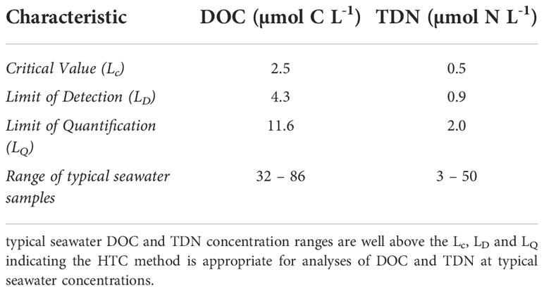
Table 1 Method validation results for analysis of DOC and TDN in seawater using the HTC method.
6.2 Analytical quality limits
6.2.1 Accuracy
Evaluated by use of consensus reference material as a control (there is no national or international standard for seawater DOC). The community has accepted the CRM distributed by the Hansell Laboratory, Rosenstiel School of Marine and Atmospheric Science (RSMAS), University of Miami. Concentrations should remain within range of consensus values (as reported by Hansell Lab: https://hansell-lab.rsmas.miami.edu/consensus-reference-material/index.html) to within ± 2% (for DOC) and ± 2-6% for TDN (depending on the concentration range).
6.2.2 Precision – repeatability and reproducibility
6.2.2.1 Repeatability
Best achievable internal precision can be assessed through repeated observations of replicate sample vials over a short period of time. Conditions such as instrument type and operator should remain constant.
6.2.2.2 Reproducibility
The external complement to repeatability, assessed by analyzing identical batches of samples with the same method among different laboratories to evaluate how reproducible results are. This method utilized intercomparisons performed on batches of reference waters between the Carlson and Hansell DOM labs from 2018-2019.
A summary of analytical quality limits for analysis of DOC and TDN in seawater using the HTC method can be found in Table 2. Refer to Supplementary Appendix G for additional details.
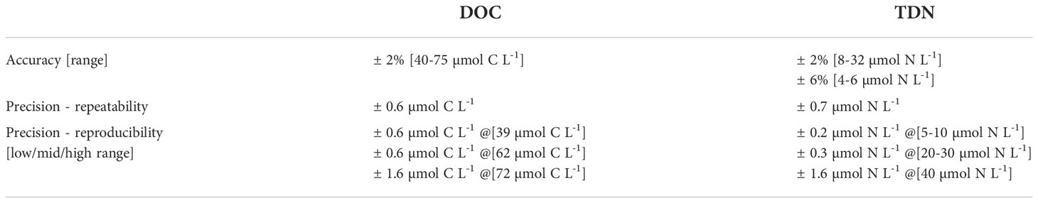
Table 2 Summary of analytical quality limits for analysis of DOC and TDN in seawater using the HTC method.
6.3 Assessing laboratory performance
As outlined in Section 4 and 5, the use of blanks, calibration standards and reference materials provide ongoing checks on instrument performance. Once validation exercises have been conducted and the method established in a laboratory ongoing assessment of data quality should occur on a frequent basis in order to maintain tight quality control. Table 3 presents a summary of recommendations for assessing DOC and TDN data runs using the HTC method as presented here.
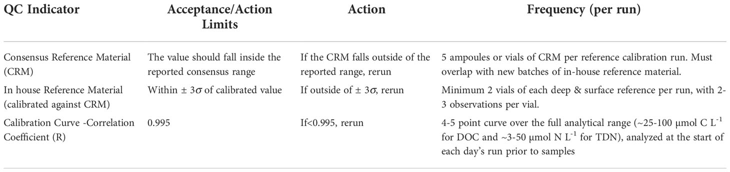
Table 3 Suggested quality control criteria and guidelines.
6.4 Quality assurance
If a run passes the QC specifications outlined above for analytical performance, then the data are accepted and further scrutinized in the context of collection and additional metadata available. If the run did not pass these initial requirements, the system is checked and the entire run is repeated.
6.5 GO-SHIP data compilation and assessment
For GO-SHIP, DOM data are compiled using shipboard logs and merged with bottle data files containing any other chemical and physical data available and then plotted in Ocean Data View (Schlitzer, R., Ocean Data View, https://odv.awi.de, 2021). Initial plots of vertical profiles and/or contour plots are helpful in identifying potential outliers. Any samples outside of a reasonable range for oceanic DOC/TDN values are flagged as potentially contaminated or suspected of handling error (values< 30 or > 90 µmol C kg-1,< 3 or > 50 µmol N kg-1).
Flagged samples are either compared against replicates or re-analyzed to confirm. If analytical errors are suspected, entire profiles or sample subsets (including problematic value and surrounding samples) are re-analyzed. Upon re-analysis of sample, if analytical specifications are met and data remain anomalously high or low then the data are reported but flagged as questionable or bad according to World Ocean Circulation Experiment (WOCE) quality flag codes (refer to Table 4).
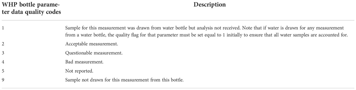
Table 4 Woce Hydrographic Program (WHP) bottle parameter data quality codes (https://www.nodc.noaa.gov/woce/woce_v3/wocedata_1/whp/exchange/exchange_format_desc.htm).
6.6 Interlaboratory data comparisons
It is recommended that samples and references be shared periodically between analytical groups to ensure interlaboratory comparability. Figure 1 is an example of intercomparisons between the University of Miami and UCSB DOM laboratories.
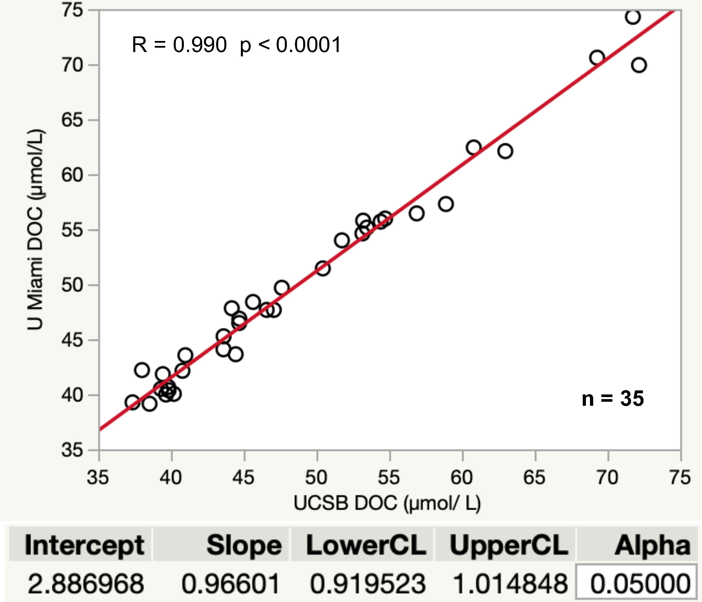
Figure 1 Results of interlaboratory comparisons conducted between UCSB and University of Miami between 2017- 2018. Samples include comparisons of CRMs, in-house references, and field profiles collected from various locations in the Pacific and Atlantic Oceans. Samples were shared equally between the groups for analysis. Correlation coefficient shows a strong relationship between UCSB and UMIAMI data (R = 0.990, p< 0.001). Orthogonal regression (univariate variances, prin comp) using JMP software (JMP®, Version<15>. SAS Institute Inc., Cary, NC, 1989–2021) gives a 0.919-1.015 confidence interval for the slope, which includes 1.0 and shows strong agreement between the values reported by each laboratory across a broad dynamic range, providing confidence in accurate and precise results for GO-SHIP data collected and analyzed as described in this best practices guide.
7 Documentation
7.1 DOM analysis reports
The following are examples of metadata which can be included in DOM cruise reports:
● Cruise designation and principal investigator(s)
● Names and affiliations of technicians who collected DOM samples at sea
● Number of stations occupied and samples collected (sampling frequency)
● Sampling and storage procedures
● Names and affiliations of technicians who analyzed DOM samples on-shore
● Number of samples analyzed
● Methods of analysis (equipment & methodology)
● Data processing procedures and Quality Control (calculations, accuracy, precision and detection limits, CRM information)
● Any details of problems or trouble-shooting that occurred with sampling or analysis
● Scientific references
7.2 Bottle data files
Data from DOM analysis (DOC and TDN) is merged with CLIVAR and Carbon Hydrographic Data Office (CCHDO) bottle exchange files based on sample identifiers (station/cast/depth/bottle ID).
Once data are merged with other chemical parameters in the bottle file, dissolved organic nitrogen (DON) is calculated as the difference between TDN and DIN . As DON is a derived variable, it is not reported (i.e., not included in the bottle file).
Final results are reported in units of μmol kg-1. Where possible direct measures of sample salinity and analytical temperature are used to calculate average seawater density. In practice we have found that applying an average seawater density of 1.027 kg m-3 to open ocean water column DOM samples, compared to direct measure of sample density results in a difference of less than 0.01 µmol kg-1 (i.e., less than analytical resolution). However, when salinity and an average analytical lab temperature are available or in regions where salinity varies strongly, a more accurate density correction is determined and applied for each sample. Each parameter includes a field for quality control flags.
8 Conclusion
The methodology presented here aims to provide the marine science community with the details required to consistently produce high quality data for analysis of dissolved organic carbon and total dissolved nitrogen in seawater samples. These best practices were written for the GO-SHIP Repeat Hydrography Practices Collection (Halewood et al., 2022) but are applicable to a wide variety of programs, ranging from focused study sites and time series to global observation networks and hydrographic ship based surveys.
Data availability statement
The raw data supporting the conclusions of this article will be made available by the authors, without undue reservation.
Author contributions
EH coordinated and carried out the final review and completion of the manuscript. All authors contributed to the writing of the initial manuscript and EH, KO, LC, DH, and CC provided reviews and contributions to the revised versions and share first authorship. All authors contributed to the article and approved the submitted version.
Funding
Support for this work was provided by the U.S. National Science Foundation (NSF OCE 1436748 to DAH, OCE 2023500 to CAC) and Simons Foundation International BIOS-SCOPE program to CAC. NASA EXPORTS Award 80NSSC18K0437 to CAC.
Acknowledgments
This manual was written by technical teams at the University of California Santa Barbara (Craig Carlson Microbial Oceanography Lab) and University of Miami (Dennis Hansell Organic Biogeochemistry Lab). The authors thank the technical staff, students and field teams in the Carlson and Hansell labs over the years who contributed to the development of these methods. Thank you also to Juliet Hermes of the Global Ocean Observing System (GOOS Task Team on Best Practices lead) and the Ocean Best Practices System (OBPS) for guidance on developing and sharing best practices for the ocean community. The authors would also like to acknowledge and thank the following scientific colleagues for extensive review of the manuscript and constructive comments and suggestions for improvement:
Boris Koch, Rik Wanninkhof, Youhei Yamashita
Conflict of interest
The authors declare that the research was conducted in the absence of any commercial or financial relationships that could be construed as a potential conflict of interest.
Publisher’s note
All claims expressed in this article are solely those of the authors and do not necessarily represent those of their affiliated organizations, or those of the publisher, the editors and the reviewers. Any product that may be evaluated in this article, or claim that may be made by its manufacturer, is not guaranteed or endorsed by the publisher.
Supplementary material
The Supplementary Material for this article can be found online at: https://www.frontiersin.org/articles/10.3389/fmars.2022.1061646/full#supplementary-material
References
Aluwihare L. I., Meador T. (2008). ““Chemical composition of marine dissolved organic nitrogen,”,” in Nitrogen in the marine environment. Eds. Capone D. G., Bronk D. A., Mulholland M. R., Carpenter E. J. (Burlington, MA: Academic Press), 95–140.
Baetge N., Behrenfeld M. J., Fox J., Halsey K. H., Mojica K. D. A., Novoa A., et al. (2021). The seasonal flux and fate of dissolved organic carbon through bacterioplankton in the Western north Atlantic. Front. Microbiol. 12, 669883. doi: 10.3389/fmicb.2021.669883
Benner R., Strom M. (1993). A critical evaluation of the analytical blank associated with DOC measurements by high-temperature catalytic oxidation. Mar. Chem. 41, 153–160. doi: 10.1016/0304-4203(93)90113-3
Bronk D. A. (2002). ““Dynamics of DON,”,” in Biogeochemistry of marine dissolved organic matter, 1st ed. Eds. Hansell D. A., Carlson C. A. (San Diego, CA: Academic Press), 153–247.
Carlson C. A., Ducklow H. W., Hansell D. A., Smith W. O. (1998). Organic carbon partitioning during spring phytoplankton blooms in the Ross Sea polynya and the Sargasso Sea. Limnol. Oceanogr. 43, 375–386. doi: 10.4319/lo.1998.43.3.0375
Carlson C. A., Ducklow H. W., Michaels A. F. (1994). Annual flux of dissolved organic carbon from the euphotic zone in the northwestern Sargasso Sea. Nature 371, 405–408. doi: 10.1038/371405a0
Carlson C. A., Hansell D. A., Nelson N. B., Siegel D. A., Smethie W. M., Khatiwala S., et al. (2010). Dissolved organic carbon export and subsequent remineralization in the mesopelagic and bathypelagic realms of the north Atlantic basin. Deep-Sea. Res. II. 57, 1433–1445. doi: 10.1016/j.dsr2.2010.02.013
Cauwet G. (1978). Organic chemistry of seawater particulates. concepts and developments. Oceanol. Acta 1 (1), 99–105.
Eppley R. W., Stewart E., Abbott M. R., Owen R. W. (1987). Estimating ocean production from satellite-derived chlorophyll: insights from the eastropac data set. Oceanol. Acta SP, 109–113.
Fasham M. J. R., Balino B. M., Bowles M. C., Anderson R., Archer D., Bathmann U., et al. (2001). A new vision of ocean biogeochemistry after a decade of the joint global ocean flux study (JGOFS). Ambio 30 (SPEC. ISS. 10), 4–31.
Halewood E., Opalk K., Custals L., Carey M., Hansell D. A., Carlson C. A. (2022) GO-SHIP repeat hydrography: Determination of dissolved organic carbon (DOC) and total dissolved nitrogen (TDN) in seawater using high temperature combustion analysis. Available at: https://repository.oceanbestpractices.org/handle/11329/1921.
Hansell D. A. (1993). Results and observations from the measurement of DOC and DON using high temperature catalytic combustion techniques. Mar. Chem. 41, 195–202. doi: 10.1016/0304-4203(93)90119-9
Hansell D. A. (2005). Dissolved organic carbon reference material program. Eos. Transactions. Am. Geophys. Union. 86 (35), 318. doi: 10.1029/2005EO350003
Hansell D. A., Carlson C. A. (1998). Deep ocean gradients in dissolved organic carbon concentrations. Nature 395, 263–266. doi: 10.1038/26200
Hansell D. A., Carlson C. A., Amon R. M. W., Alvarez-Salgado X. A., Yamashita Y., Romera-Castillo C., et al. (2021). Compilation of dissolved organic matter (DOM) data obtained from the global ocean surveys from 1994 to 2020 (NCEI accession 0227166) (NOAA National Centers for Environmental Information) (MD, USA: Silver Spring). doi: 10.25921/s4f4-ye35
Hansell D. A., Carlson C. A., Repeta D. J., Shlitzer R. (2009). Dissolved organic matter in the ocean: A controversy stimulates new insights. Oceanography 22, 202–211. doi: 10.5670/oceanog.2009.109
Hansell D. A., Carlson C. A., Schlitzer R. (2012). Net removal of major marine dissolved organic carbon fractions in the subsurface ocean. Global Biogeochem. Cycles. 26 (1), [GB1016]. doi: 10.1029/2011GB004069
International Union of Pure and Applied Chemistry (1995). Nomenclature in evaluation of analytical methods, including detection and quantification capabilities (IUPAC recommendations 1995). Pure. Appl. Chem. 67 (10), 1699–1723. doi: 10.1351/pac199567101699
Knap A., Michaels A., Close A., Ducklow H., Dickson A. (1996). “Protocols for the joint global ocean flux study (JGOFS) core measurements,” in JGOFS, reprint of the IOC manuals and guides no. 29 (UNESCO) (Paris, France).
Letscher R. T., Hansell D. A., Carlson C. A., Lumpkin R., Knapp A. N. (2013). Dissolved organic nitrogen in the global surface ocean: Distribution and fate. Global Biogeochem. Cycles. 27, 141–153. doi: 10.1029/2012GB004449
Liu S., Longnecker K., Kujawinski E. B., Vergin K., Bolaños L. M., Giovanonni S. J., et al. (2022). Linkages among dissolved organic matter export, dissolved metabolites, and associated microbial community structure response in the northwestern Sargasso Sea on a seasonal scale. Front. Microbiol. 13, 833252. doi: 10.3389/fmicb.2022.833252
MacKenzie F. T. (1981). “Global carbon cycle: Some minor sinks for CO2.” in Flux of organic carbon by rivers to the ocean. Eds. Likens G. E., MacKenzie F. T., Richey J. E., Sedell J. R., Turekian K. K. (Washington, DC: U.S. Dept. of Energy), 360–384.
Mopper K., Qian J. (2006). “Water analysis: Organic carbon determinations,” in Encyclopedia of analytical chemistry, online © 2006 (John Wiley & Sons, Ltd) (Hoboken, NJ).
Novak M. G., Cetinić I., Chaves J. E., Mannino A. (2018). The adsorption of dissolved organic carbon onto glass fiber filters and its effect on the measurement of particulate organic carbon: A laboratory and modeling exercise. Limnol. Oceanogr.: Methods 16, 356–366. doi: 10.1002/lom3.10248
Peltzer E. T., Brewer P. G. (1993). Some practical aspects of measuring DOC – sampling artifacts and analytical problems with marine samples. Mar. Chem. 41 (1-3), 243–252. doi: 10.1016/0304-4203(93)90126-9
Ridgwell A., Arndt S. (2014). “Why dissolved organics matter: DOC in ancient oceans and past climate change,” in Biogeochemistry of marine dissolved organic matter, 1st ed. Eds. Hansell D. A., Carlson C. A. (San Diego, CA: Academic Press), 1–19.
Schlitzer R. (2021) Ocean data view. Available at: https://odv.awi.de.
Sharp J. H. (1993). The dissolved organic carbon controversy: an update. Oceanography 6, 45–50. doi: 10.5670/oceanog.1993.13
Sharp J. H., Benner R., Bennett L., Carlson C. A., Fitzwater S. E., Peltzer E. T., et al. (1995). Analyses of dissolved organic carbon in seawater: the JGOFS EqPac methods comparison. Mar. Chem. 48, 91–108. doi: 10.1016/0304-4203(94)00040-K
Sharp J. H., Carlson C. A., Peltzer E. T., Castle-Ward D. M., Savidge K. B., Rinker K. R. (2002a). Final dissolved organic carbon broad community intercalibration and preliminary use of DOC reference materials. Mar. Chem. 77 (4), 239–253. doi: 10.1016/S0304-4203(02)00002-6
Sharp J. H., Rinker K. R., Savidge K. B., Abell J., Benaim J. Y., Bronk D., et al. (2002b). A preliminary methods comparison for measurement of dissolved organic nitrogen in seawater. Mar. Chem. 78 (4), 171–184. doi: 10.1016/S0304-4203(02)00020-8
Tappin A. D., Nimmo M. (2019). “Water analysis | seawater: Dissolved organic carbon.” in Encyclopedia of analytical science, 3rd ed. Eds. Worsfold ,. P., Poole ,. C., Townshend ,. A., Miró ,. M., 345–352. (Cambridge, MA: Elsevier)
Turnewitsch R., Springer B. M., Kiriakoulakis K., Vilas J. C., Aristegui J., Wolff G., et al. (2007). Determination of particulate organic carbon (POC) in seawater: The relative methodological importance of artificial gains and losses in two glass-fiber-filter-based techniques. Mar. Chem. 105, 208–228. doi: 10.1016/j.marchem.2007.01.017
Walsh T. W. (1989). Total dissolved nitrogen in seawater: a new high-temperature combustion method and a comparison with photo-oxidation. Mar. Chem. 26, 295–311. doi: 10.1016/0304-4203(89)90036-4
Williams P. M., Druffel E. R. M. (1987). Radiocarbon in dissolved organic matter in the central north pacific ocean. Nature 330, 246–248. doi: 10.1038/330246a0
Keywords: dissolved organic carbon (DOC), total dissolved nitrogen (TDN), dissolved organic matter, high temperature combustion analysis, GO-SHIP, best practices, methodology
Citation: Halewood E, Opalk K, Custals L, Carey M, Hansell DA and Carlson CA (2022) Determination of dissolved organic carbon and total dissolved nitrogen in seawater using High Temperature Combustion Analysis. Front. Mar. Sci. 9:1061646. doi: 10.3389/fmars.2022.1061646
Received: 04 October 2022; Accepted: 23 November 2022;
Published: 12 December 2022.
Edited by:
Juliet Hermes, South African Environmental Observation Network (SAEON), South AfricaReviewed by:
Elizabeth Minor, University of Minnesota Duluth, United StatesMorimaru Kida, Kobe University, Japan
Copyright © 2022 Halewood, Opalk, Custals, Carey, Hansell and Carlson. This is an open-access article distributed under the terms of the Creative Commons Attribution License (CC BY). The use, distribution or reproduction in other forums is permitted, provided the original author(s) and the copyright owner(s) are credited and that the original publication in this journal is cited, in accordance with accepted academic practice. No use, distribution or reproduction is permitted which does not comply with these terms.
*Correspondence: Elisa Halewood, d2FsbG5lckB1Y3NiLmVkdQ==; Craig A. Carlson, Y3JhaWdfY2FybHNvbkB1Y3NiLmVkdQ==