 Jisun Shin1
 So-Hyun Kim
 Boo-Keun Khim
 Young-Heon Jo
- 1BK21 School of Earth and Environmental System, Pusan National University, Busan, Republic of Korea
- 2Department of Ocean Engineering, University of New Hampshire, Durham, NH, United States
Floating Sargassum horneri has flowed into Jeju Island and the coast of the Korean Peninsula every year between February and May since 2015, causing considerable damage to aqua-farming sites and navigation. This study aimed to address the relationship between Sargassum distribution in the Yellow Sea (YS) and the East China Sea (ECS) and environmental variables for determining Sargassum distribution toward the Korean Peninsula. From feature importance ranking, we found that sea surface temperature (SST) is the most influential environmental variable in Sargassum distribution. From variables such as sea surface height (SSH), eastward seawater velocity (uo), and northward seawater velocity (vo), it was observed that Sargassum patches were not distributed in the southeast below 29 °N. Subsequently, we employed bagged tress models to evaluate the specific sensitivity of each environmental variable to Sargassum distribution. This model showed the best quantitative and qualitative performance when trained with physical and geographical variables. When estimating expanded areas of Sargassum distribution over time with the change in SST, a sider distribution range of Sargassum patches than usual and an early inflow into the Korean Peninsula were observed when the SST increased from the original. In addition, we found that the tolerable and favorable SST for Sargassum was 12–20 and 18°C, respectively. These results will enhance the understanding of the relationship between environmental variables and Sargassum distribution and provide valuable data for establishing a pre-disaster system for Sargassum blooms flowing toward the Korean Peninsula.
Introduction
The golden tides found in the East China Sea (ECS) and Yellow Sea (YS) have been attributed to Sargassum horneri (Liu et al., 2018; Xing et al., 2018; Zhang et al., 2019). The floating golden tide has been reported in the ECS since the early 2000s and has frequently appeared in the YS (Qi et al., 2017). The gas-filled bladder-like vesicles on the thalli of Sargassum provide buoyancy and allow them to float (Xu et al., 2016). Komatsu et al. (2007a); Komatsu et al. (2007b) observed pelagic Sargassum on a research vessel during a field survey in the ECS and the Kuroshio Current. It has been increasingly sighted over the past two decades. In 2015, a large amount of Sargassum flowed into waters around the Korean Peninsula. It can be wound around ship screws and cause loss of Pyropia yezoensis aquaculture (Zhuang et al., 2021). In addition, its odor harms the sightseeing and scenery of the beach. Therefore, if Sargassum is collected before it enters a coastal area or fish farm, its effect can be reduced. Sargassum has been collected in Korea by the Ministry of Oceans and Fisheries (MOF). After its appearance in 2015, the disposal cost of Sargassum was $ 1.6 million to remove 33,439 tons by 2020, although it has varied from year to year (Press). Despite the pledge for detailed preparation and preemptive response to the massive influx of Sargassum, clear guidelines for damage prevention and response still need to be provided.
Several studies have attempted to identify the migration pathways of golden tides using field surveys, satellite detection, and particle tracking models (Chen et al., 2019; Kim et al., 2019; Yuan et al., 2022). Mizuno et al. (2014) investigated the distribution and migration of golden tides through field surveys using a research vessel. Considering the surface currents and geophysical distribution of Sargassum during that period, they assumed that the central and southern coasts of China were the origin. Qi et al. (2017) traced the source of floating algae blooms using satellite images and numerical particle-tracking experiments. They suggested that one of bloom origin is in offshore of the Zhejiang coast in 2017. Subsequently, they found that the initial Sargassum patches move to northeast YS. Using particle tracking numerical experiments, Lee (2018) reported that Sargassum patches found on Jeju Island originated from two regions of China. Patches found on northern Jeju Island originated from the Shandong Peninsula between December and January, while patches found on southern Jeju Island originated from the Jiangsu province between late January and mid-February. Kwon et al. (2019) reproduced the trajectories of Sargassum patches using Lagrangian particle-tracking simulations and three-dimensional circulation modeling. They attempted backward particle tracking from May to April 2017 to determine the location of Sargassum patch a month earlier and found that the synthetic particles were translated southwestward.
In addition, some studies have revealed various environmental factors that may affect the distribution and migration of Sargassum. Wu et al. (2019) reported that temperature had a significant impact on photosynthesis, carbon assimilation, growth, and the life cycle of Sargassum. Komatsu et al. (2007a) observed drifting Sargassum in areas where the sea surface temperature (SST) was 20–24 °C. Qi et al. (2017) reported that a higher SST in 2017 could stimulate faster Sargassum growth compared to that in previous years, thereby leading to an unprecedented bloom in 2017. In particular, they suggested that a slight increase of SST by 0.5–1 °C along Zhejiang coast in 2017 may stimulate initial Sargassum growth. Zheng et al. (2022) analyzed the correlation between the sea surface temperature anomaly (SSTA) and the growth rate of Sargassum. They reported that the growth rate of Sargassum increased with increasing SSTA in May. In addition, the trajectories and distribution of Sargassum patches are controlled by wind and surface currents. Employing a sensitivity simulation of the particle tracking model, Kwon et al. (2019) confirmed that southern wind contributed to the further northward movement of Sargassum patches to the YS in May 2017. Kim et al. (2019) analyzed the migration of Sargassum patches using Hybrid Coordinate Ocean Model (HYCOM) surface current data. Yuan et al. (2022) examined the impacts of wind vectors on the development and drifting of floating Sargassum in the YS and ECS. They found that the drifting direction of the floating patches was consistent with the prevailing wind vectors. These studies have investigated the individual environmental factors of the waters where Sargassum patches were observed in an approximate spatial and time-series rather than focusing on the instantaneous environmental factors of the waters where Sargassum patches exist. Therefore, it is essential to determine the importance by considering all possible factors rather than individual environmental factors that affect Sargassum distribution. Furthermore, it will be necessary to analyze the relationship between Sargassum distribution and factors and understand how much each factor affects Sargassum distribution.
This study addresses the relationship between Sargassum distribution and environmental factors that may affect Sargassum distribution in the YS and ECS. We first generated a daily Sargassum map using a particle tracking model and satellite images. The feature importance of the environmental data affecting Sargassum distribution was investigated. A machine learning model was trained and tested to estimate Sargassum distribution from the environmental data. We then analyzed Sargassum distribution according to the changing environmental variables.
Study area
The study area includes the ECS and the YS, 119–129°E and 26–35°N (Figure 1A). The ECS is an arm of the western Pacific Ocean that extends directly from East China. The northern extension between mainland China and the Korean Peninsula is the YS. The Yangtze River, the biggest river in China, is the largest in East Asia (Yang et al., 2011). As the major channel connecting the Yangtze River and the ECS, the Yangtze River Estuary is influenced by strongly varying river discharges and moderate tides (Yun, 2004). In addition, the Kuroshio is a western boundary current in the North Pacific that flows northeastward after entering the southeast ECS (Kang and Na, 2022). It has significant effects on both the physical and biological processes of the North Pacific, including nutrient and sediment transport, regional climate, and Pacific mode water formation (Hu et al., 2015; Das et al., 2021). The Tsushima Current diverges from the Kuroshio Current in the ECS, flows into the East Sea in Korea, and moves northward along the East Sea. Most of the ECS is shallow, with approximately three-fourths less than 200 m deep, with an average depth of 350 m. Within the study area, the origin of Sargassum bloom is generally offshore from the Zhejiang coast. Patches along the Kuroshio Current and Taiwan Warm Current move to the northeast. Then, it reaches Jeju Island or the YS. The Geostationary Ocean Color Imager (GOCI) image in Figure 1B was obtained on April 23, 2017, when a large-scale Sargassum patch appeared in the study area. The patch was red in the Rayleigh-corrected reflectance (RhoC) pseudo-color composite (R: 865 nm; G: 680 nm; B: 555 nm). However, it was difficult to recognize Sargassum patch clearly due to the cloud and turbid waters white color.
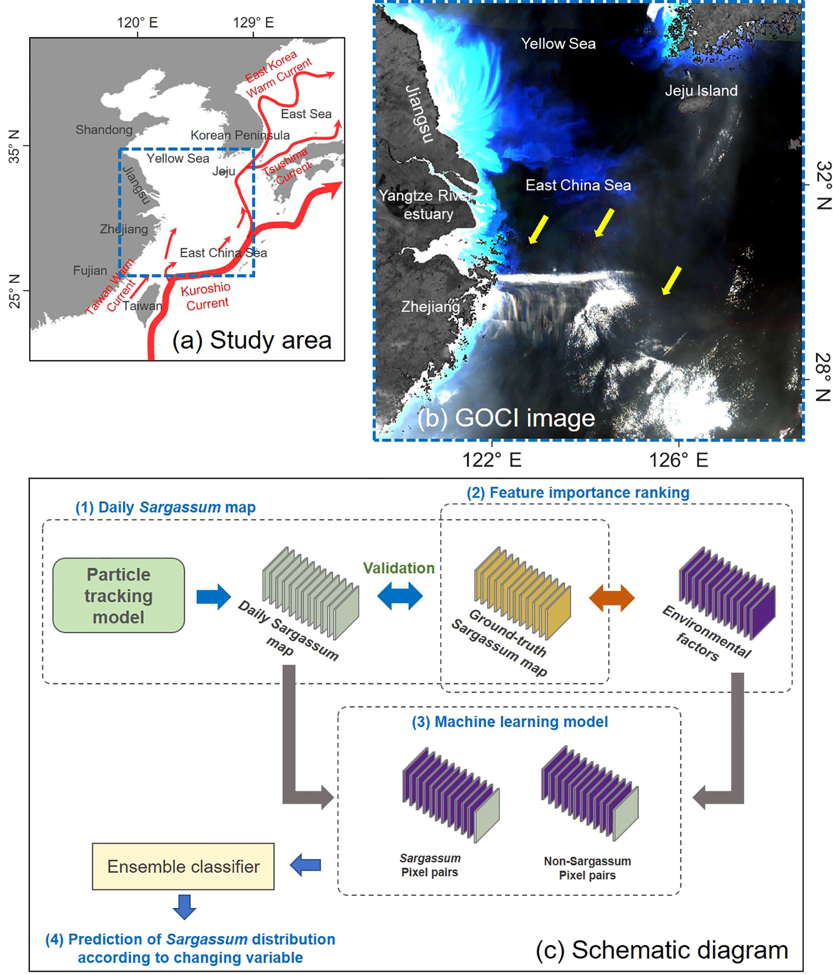
Figure 1 Study area and schematic diagram in this study. (A) The study area covers the East China Sea (ECS) and the southern Yellow Sea (YS) including Jeju Island in Korea. (B) Rayleigh-corrected reflectance (RhoC) pseudo-color composite image generated from Geostationary Ocean Color Imager (GOCI) acquired on April 23, 2017 at 02:16 UTC. The patch in red is recognized as Sargassum (yellow arrow). (C) Schematic showing the relationship between Sargassum distribution and environmental factors. There are the four steps are: (1) The daily Sargassum maps were generated using ground-truth Sargassum data and particle tracking model, (2) feature importance ranking was performed for investigating the importance between environmental factors affecting Sargassum distribution, (3) machine learning model was trained and tested for predicting Sargassum distribution through environmental factors, and (4) Sargassum distribution was predicted according to changing environmental variables using the machine learning model.
Materials and methods
Figure 1C shows a schematic diagram of the relationship between Sargassum distribution and environmental factors. We generated a daily Sargassum map from 2015 to 2019 using the ground-truth Sargassum map derived from GOCI image and particle tracking model. Feature importance ranking (FIR) was conducted to investigate the feature importance among the eight environmental factors affecting Sargassum distribution. The environmental factors were divided into two groups based on physical factors. The first group includes SST and seawater salinity (SS), which affect the physiology of Sargassum. The second group is composed of sea surface height (SSH), seawater density (rho), seawater current, and wind stress, which can affect the migration of Sargassum patches. We used matching pairs between environmental data and Sargassum or non-Sargassum pixels of the ground truth. Thereafter, the machine learning models were trained and tested using Sargassum and non-Sargassum pixel pairs. These pairs consist of Sargassum or non-Sargassum pixels extracted from daily Sargassum maps and the corresponding environmental data. Finally, we predicted Sargassum distribution according to changing environmental variables using the trained machine learning model.
Particle tracking model for daily Sargassum map
To generate a daily Sargassum map, we conducted a particle-tracking experiment developed by Choi et al. (2018) based on the fourth-order Runge-Kutta scheme. They derived new velocity fields based on satellite measurements and calculated the velocity fields by combining Ekman currents and geostrophic currents based on an analytical solution of an approximated momentum equation (Welander, 1957). The trajectories of surface-floating substances estimated from new velocity fields can be reasonably simulated experimentally. The initial distribution of Sargassum patches is essential to estimate the trajectory of Sargassum patch using a particle tracking model. For this purpose, we used GOCI images as ground truth data. Although satellite observations have the advantage of providing information over a wide area, they are often hampered by weather conditions (Zhang et al., 2019). Therefore, in this study, GOCI images were used to provide the initial distribution and validation of the particle-tracking model. We used RhoC GOCI products downloaded from the Korea Ocean Satellite Center (https://kosc.kiost.ac.kr/). GOCI image has a spatial resolution with 500 m. Images were obtained eight times per day between 0 to 7 UTC. We used GOCI images taken at 2 UTC. The total coverage of the image was 2500 × 2500 km in Northeast Asia. The normalized difference vegetation index (NDVI) (Rouse et al., 1974), which expresses the optical properties of Sargassum, was used to extract Sargassum pixels from GOCI images. The NDVI was calculated using the following equation:
where NIR is the near-infrared wavelength band (865 nm), and RED is the red wavelength band (680 nm). A pixel with positive value was identified as Sargassum. Table 1 lists information related to Sargassum pixels extracted from GOCI images. A total of 10,996 pixels were extracted between 2015 and 2019. The distribution of the pixels extracted from GOCI image, where Sargassum patch was first found every year, was set as the initial distribution. The remaining images were used to validate the model. To generate Sargassum map, the latitude and longitude data of extracted Sargassum pixels were converted to 1/12° consistent with spatial resolution of environmental data.

Table 1 Information of ground-truth data obtained from GOCI images.
To set the model parameters, the time step and number of calculation steps over 100 days were set to 150 min and 960, respectively. The time step is expected to sufficiently satisfy the stability condition of advection given by . ere . the maximum speed of the current, Δ t is the time step, and △x≈20 km . the spatial resolution of the velocity field. We conducted a particle-tracking experiment to trace Sargassum patches. Synthetic particles were released on the initial date each year. Daily Sargassum maps from 2015 to 2019 were generated using this model. To validate the location of Sargassum pixels derived from the model domain, buffer areas were designated by two pixels around each Sargassum pixel. We calculated a confusion matrix between the synthetic particle and the matched Sargassum patch for each synthetic particle (Kohavi, 1998). Notably, if the distance was more than 40 km, the synthetic particles were considered with inconsistent matching Sargassum pixels. Sargassum pixels in the ground truth were either true (sr) or false (nsr), whereas the synthetic particles were designated as true (SR) or false (nSR). This consists of four categories: (1) sr classified as SR (true positive), (2) sr classified as nSR (false negative), (3) nsr classified as SR (false positive), and (4) nsr classified as nSR (true negative). The performance of the particle tracking model was evaluated using sensitivity ((1)/[(1)+(2)]) and precision ((1)/[(1)+(3)]). In addition, F-measure was used to describe the total accuracy as the following equations:
We evaluated the performance of the particle tracking model for estimating the daily Sargassum map. As a result, the sensitivity and precision of the model were 0.36 and 0.46, respectively. The F-measure and total accuracy showed a good level with 0.41 and 0.82, respectively.
Environmental data
The Global Ocean Physics Reanalysis of the Copernicus Marine Environment Monitoring Service (CMEMS) product (GLOBAL_MULTIYEAR_PHY_001_030) was used in this study (Gounou et al., 2020) (https://resources.marine.copernicus.eu/products). This product includes daily and monthly mean files for temperature, salinity, currents, sea level, mixed layer depth, and ice parameters from top to bottom. The global ocean output files were displayed on a standard regular grid at 1/12° (approximately 8 km) and 50 standard levels. We used SST, SS, SSH, eastward horizontal velocity (uo), and northward horizontal velocity (vo) with a depth of 0.49 m. The European Center for Medium-range Weather Forecasts (ECMWF) Reanalysis v5 (ERA5) provides an eastward component of 10 m wind and a northward component of 10 m wind datasets at approximately 25 km × 25 km (1/4° × 1/4°). We calculated the eastward (wsu) and northward wind stress (wsv) from the wind data using the following equation:
where ρα is the air density, CD is the drag coefficient, and Vα is the wind speed 10 m above the sea surface (Trenberth et al., 1990). The data period was from January 1, 2015 to December 31, 2019, per day. To match the spatial resolution between the CMEMS and ERA5 data, we resampled the spatial resolution of both data into daily 8 km × 8 km. To calculate rho, we used the Gibbs-SeaWater (GSW) v3.06 Oceanographic Toolbox (https://www.teos-10.org/). It contains the thermodynamic equation of seawater (TEOS)-10 subroutines to evaluate the thermodynamic properties of pure water and seawater. TEOS-10 is based on a Gibbs function formulation in which all thermodynamic properties of seawater can be derived in a thermodynamically consistent manner (McDougall and Barker, 2011). We calculated rho from SST, SS, and sea pressure using the GSW function. Here, the sea pressure was assumed to be at the sea surface and set to 0.
Feature importance ranking
For the FIR, the pairs between Sargassum or non-Sargassum pixels of the ground truth and the corresponding environmental data were matched. Non-Sargassum pixels were randomly extracted five times (54,980 pixels) from 10,996 Sargassum pixels (Table 1) from each image. A total of 10,994 Sargassum and 53,398 non-Sargassum pixels were used for the FIR, except for the number value among the matched pairs. In machine learning, FIR refers to a task that measures the contributions of individual input variables to the performance of a supervised learning model (Samek et al., 2017). FIR is a powerful tool in explainable or interpretable artificial intelligence to facilitate understanding of decision-making by a learning system (Wojtas and Chen, 2020). Among the feature-ranking algorithms, we used the minimum redundancy maximum relevance (mRMR) algorithm (Ding and Peng, 2005). The mRMR algorithm determines an optimal set of features that are mutually and maximally dissimilar. It minimizes the redundancy of a feature set and maximizes relevance of a feature set to the response variable. The algorithm quantifies the redundancy and relevance using the mutual information of the variables (Ding and Peng, 2005).
Machine learning model for estimating Sargassum distribution
We trained and tested the machine learning model to estimate Sargassum distribution from the environmental data. Table 2 summarizes the machine learning models used in this study. We selected bagged trees (BT) with the learner type of decision tree. Bagging represents bootstrap aggregation. Every tree in the ensemble was grown on an independently drawn bootstrap replica of the input data (Breiman, 2001). We trained the three BT models using different input variables (Table 2). SST, SS, and rho were used as input variables common to the three models (BT-1). SST and SS are physiological and physical variables that govern the growth and extermination of Sargassum. As SST and SS calculate rho variable, it was regarded as a similar variable and used as an input for the BT-1 model. Moreover, uo, wo, and SSH related to the movement of Sargassum were added to the second model (BT-2), whereas geographical (longitude and latitude) and date information were added to the second model (BT-3). The daily Sargassum map was used as the output variable for 50 days from the start of Sargassum occurrence for each year. Further, we used 195 and 55 days of map training and testing, respectively, for a total of 250 days. For the training and test datasets, 831,540 and 223,902 pixel pairs were composed of daily Sargassum maps as ground-truth data and the corresponding environmental data, respectively. The ratios for the training and test were 79 and 21%, respectively. The non-Sargassum pixels were extracted five times using Sargassum pixels. BT-3 model with the most input variables took the longest training time of 881.76 s. The maximum number of splits and number of learners were 831,539 and 30, respectively. Bayesian optimization was used as the optimizer. In addition, three trained models were quantitatively and qualitatively tested using a test dataset. Finally, to reveal the impact of environmental factors on Sargassum distribution, we analyzed Sargassum distribution according to environmental factors using the selected model.
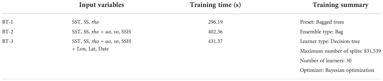
Table 2 Summary of machine learning models for estimating Sargassum distribution from environmental data.
Results
Environmental variables affecting Sargassum distribution
To identify the importance of environmental variables affecting Sargassum distribution, we calculated the FIR using the mRMR algorithm. The top eight features of the mRMR are shown in Figure 2. It was observed that the SST was the most important factor affecting Sargassum distribution, accounting for 20.8% (0.065) of all variables. The second and third most important factors were rho and uo, accounting for 14.4% (0.045) and 13.9% (0.04), respectively. The combined ratio of the top three factors was 48.1%, accounting for approximately half of the total importance. The importance scores of the factors differed up to 2.55 times. However, the remaining five factors showed similar importance in the range of 0.025–0.039. Among these factors, SSH showed a lower importance score (0.025). These results showed that not only the SST with the highest importance score, but also the remaining factors can affect Sargassum distribution.
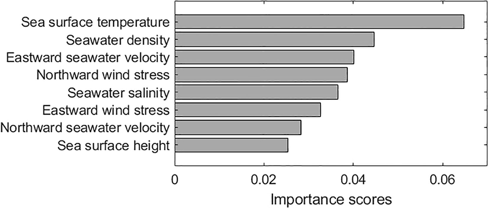
Figure 2 The rank of features in minimum redundancy maximum relevance (mRMR) algorithm for identifying the importance between environmental variables affecting Sargassum distribution. Environmental variables include sea surface temperature (SST), seawater density (rho), seawater salinity (SS), sea surface height (SSH), eastward seawater velocity (uo), and northward seawater velocity (vo), eastward wind stress (wsu), and northward wind stress (wsv).
To confirm the characteristics of the environmental variables in Sargassum and non-Sargassum groups, we investigated the distribution of eight environmental factors corresponding to these groups (Figure 3). Figure 4 shows the spatial distributions of Sargassum patches and environmental variables on April 23, 2017, when Sargassum patches were widely distributed around the Jeju coast, moving from the Zhejiang coast to the coast of the Korean Peninsula. In the case of the SST variable, the non-Sargassum group ranged from 5 to 25 °C with a bimodal distribution, while Sargassum pixels had a value between 10 and 25 °C with a normal distribution (Figure 3A). The SST histogram of Sargassum group showed a symmetrical bell-shaped distribution, whereas that of the non-Sargassum group showed a double-peak distribution. Most of Sargassum group were distributed between 14 and 18 °C. Previous studies have reported that Sargassum can grow at a wide range of temperatures between 15 and 25 °C, while the optimal growth of adult Sargassum is 14–16 °C (Mikami et al., 2006; Choi et al., 2007; Pang et al., 2009; Yuan et al., 2014; Lin et al., 2017). Yuan et al. (2022) reported that a mean SST of 8–20 °C in Sargassum blooms areas corresponded to in situ temperature range for vegetative growth and floating Sargassum. In addition, they found that SST higher than 22 °C in July-September prohibits Sargassum from blooming or completing its life cycle. In the SST distribution in Figure 4, Sargassum patches were distributed between 14 and 20 °C, which is consistent with previous results. By confirming the distribution of Sargassum at different times, we found that Sargassum patches were distributed in the same SST range even if the geographical location of Sargassum was different. The spatial distribution of SSH was similar to that of SST. The SSH of Sargassum group was mostly distributed between 0 and 0.6 m, while those of non-Sargassum group ranged from 0 to 1.2 m. In particular, Sargassum group showed low values between 0.8 and 1.2 m. These distributions show the results associated with the uo and vo distributions. Both uo and vo showed similar histogram; however, only the non-Sargassum group showed a distribution between 0.5 and 1 m/s. These results were consistent with those reported by Hsiung et al. (2022). They reported that the mean velocity of the Kuroshio along the Pacific coast of Japan was approximately 0.7–1.4 m/s. In the spatial distribution shown in Figure 4, the distribution of the high values is the point where the Kuroshio Current passes, which can be clearly identified in the uo and vo maps. Similarly, in the SSH map, the distribution of high values is shown at the same location as in the uo and vo maps. These results suggest that the distribution of Sargassum cannot move southeast due to the influence of the Kuroshio Current. As shown in Figures 4, the value range and distribution of SS were similar to those of rho. The non-Sargassum group had a lower value than Sargassum group, which was low-salinity waters around the Yangtze River (Figure 4). In the case of wind stress variables, the distribution of histograms between Sargassum and non-Sargassum groups for each variable showed no significant differences. However, the non-Sargassum groups of wsu and wsv showed a high frequency with a negative wsu value and a positive wsv value. These characteristics are shown in the wsu and wsv maps of April 23, 2017 (Figure 4).
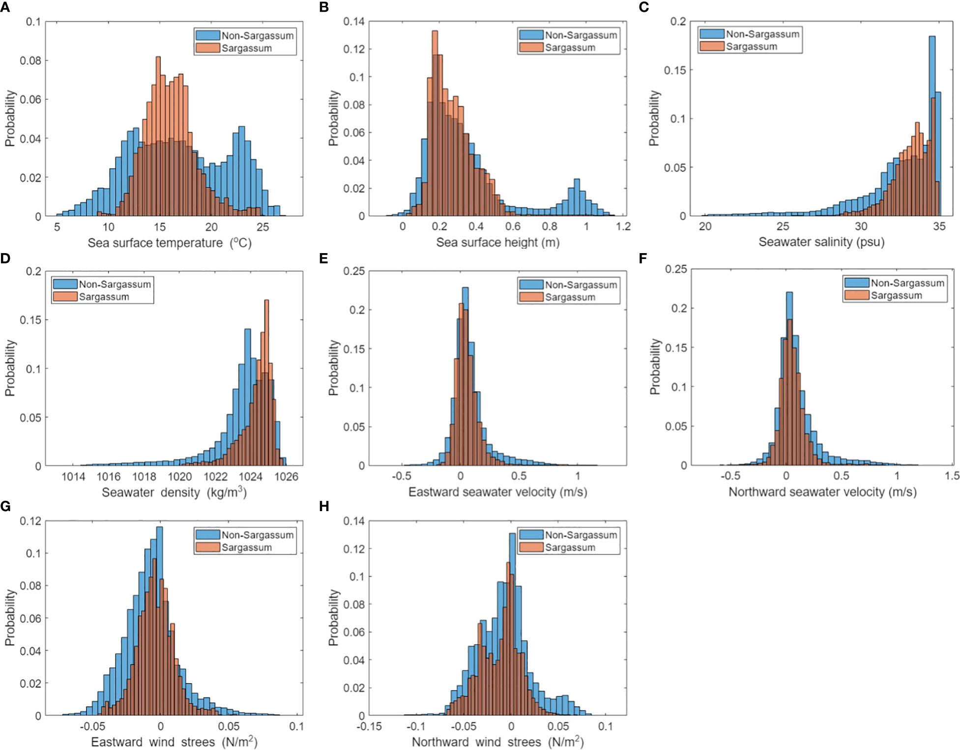
Figure 3 The histograms of Sargassum and non-Sargassum pixel groups corresponding to (A) SST, (B) SSH, (C) SS, (D) rho, (E) uo, (F) vo, (G) wsu, and (H) wsv. The pixels for each group extracted from GOCI images as ground truth data are shown in Table 1.
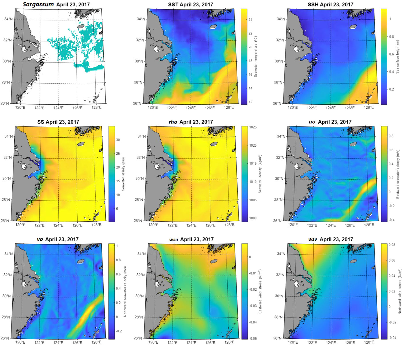
Figure 4 The distribution maps of Sargassum patches and environmental variables in the study area. Sargassum distribution as ground-truth was extracted from GOCI image on April 23, 2017.
Performance of machine learning models for Sargassum distribution
Table 3 and Figure 5 show the quantitative and qualitative performance evaluation of the three BT models with different input variables using the test dataset. In terms of quantitative evaluation, the BT-1 model showed poor performance, whereas the BT-3 model showed the best performance with an F-measure of 0.8. The sensitivity (0.76), precision (0.84), and total accuracy (0.94) of the BT-3 model were the highest among the models. Figure 5 shows the spatial distribution of the ground truth and predicted Sargassum patches using the BT models during 2016 every 15 days. We first found patches of Sargassum near the coast of Zhejiang on March 2, 2016. They were transported along the coast of the Korean Peninsula. Consistent with the results of the quantitative assessment, the BT-3 model trained with physical and geographical variables showed the most reasonable distribution. In contrast, the BR-1 model trained with only SST, SS, and rho variables showed a fairly scattered distribution, which did not simulate the movement of Sargassum patches over time. In addition to the variables used in the BT-1 model, the BT-2 model trained with the SSH and ocean currents showed an aggregated distribution compared to that of the BT-1 model. However, the initial patches still exhibited a scattered distribution. This allows us to recognize that not only physical variables, but also geographical variables have a significant impact on the performance of the model.
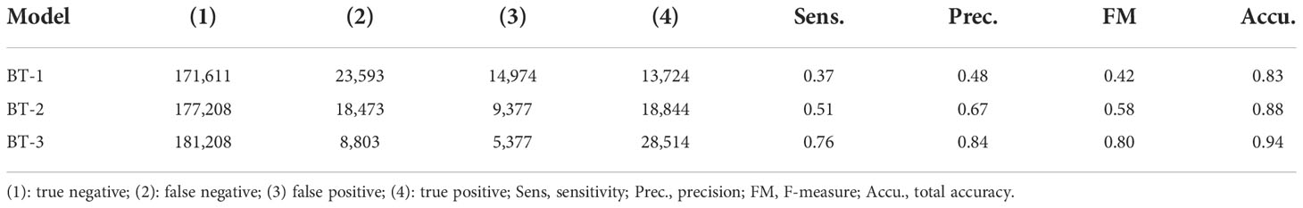
Table 3 Performance evaluation of three machine learning models using test dataset.
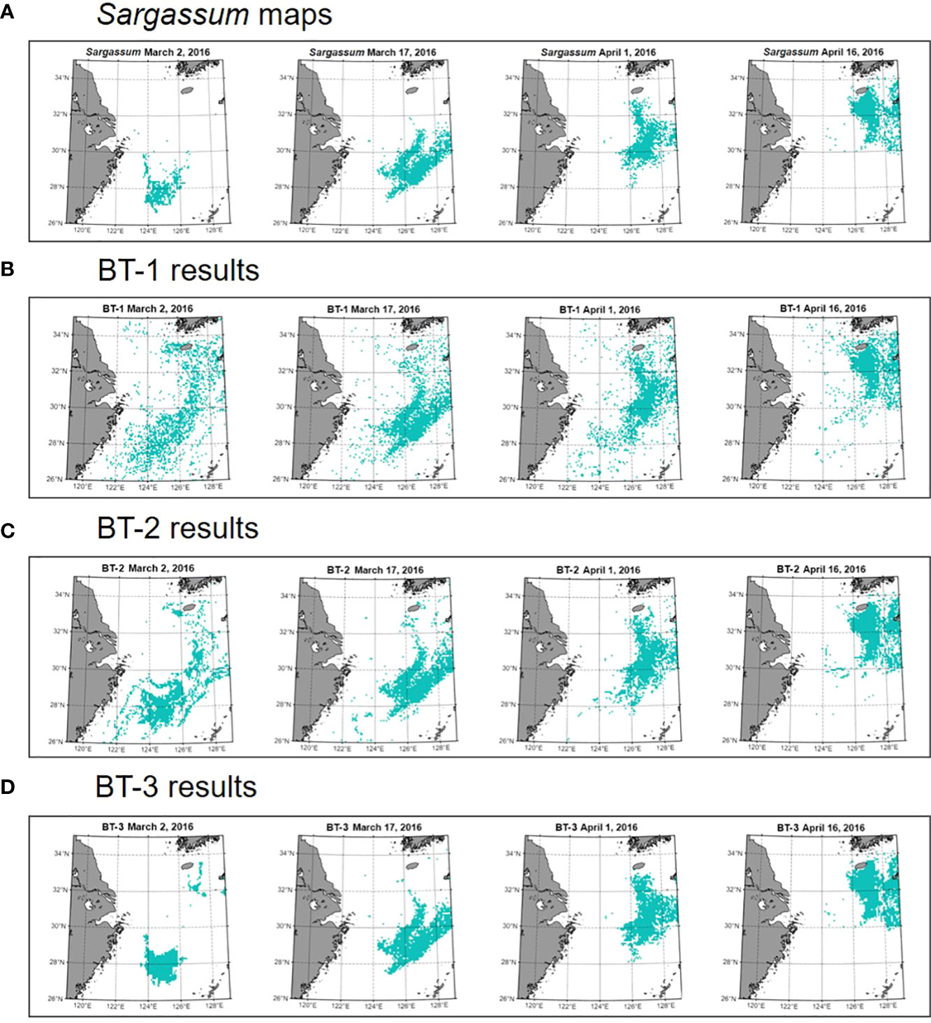
Figure 5 Sargassum map as ground truth and estimated maps derived from machine learning models (A) Daily Sargassum map was generated fromparticle tracking model. The estimated Sargassum maps generated from (B) BT-1, (C) BT-2, and (D) BT-3 models. In 2016, Sargassum patchesfirst appeared in the ECS on March 2 and gradually moved toward the Korean Peninsula. The maps are displayed every 15 days since thepatches occurred.
Sargassum distribution according to changing sea surface temperature
Through FIR analysis, we found that SST was the most important factor affecting Sargassum distribution. Therefore, to reveal the impact of SST on Sargassum distribution, we simulated five cases: (1) SST + 4 °C, (2) SST + 2 °C, (3) original SST, (3) SST − 2 °C, and (4) SST − 4 °C. These cases considered the range of SST distribution in Sargassum group. These options were applied to the BT-3 model by adjusting only the input value of the SST. We obtained continuous daily Sargassum maps for these four options. Figure 6 shows Sargassum maps according to the changing SST every 15 days in 2016. Compared with the original case (Figure 6), all cases showed a similar distribution by period. However, in the case of (1) and (2), which increased the SST from the original, additional patches were found in the initial distribution on March 2, 2016, especially around 30°N. However, this did not appear in the original distribution. Compared to cases (3) and (4), there are more patches that appear around the Korean Peninsula above 32°N over time in cases (1) and (2). In contrast, cases (3) and (4) showed a distribution in which the distribution density was reduced although the pattern was similar to that of the original patch. In particular, in case (4), the patches were closer to Jeju Island in Korea.
Figure 6 Sargassum maps according to changing SST in 2016 every 15 days. From the top to the bottom, the maps showed the results after applying four options: (A) SST + 4 °C, (B) SST + 2 °C, (C) SST − 2 °C, and (D) SST − 4 °C. The original case is represented in Figure 6.
Additionally, we calculated the expanded area of Sargassum and fitted curves according to the changing SST variable for each case (Figure 7). The equation for calculating the expanded are of Sargassum according to the yearday for each case is as follows:
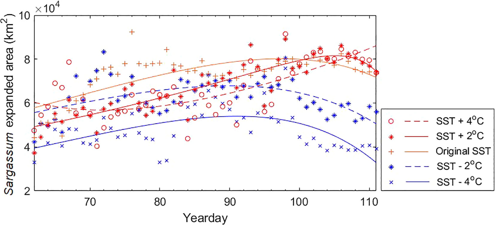
Figure 7 Sargassum expanded areas and fitted curves according to yearday for five cases in 2016 corresponding to Figure 7. Five cases include (1) SST + 4 °C, (2) SST + 2 °C, (3) original SST, (3) SST − 2 °C, and (4) SST − 4 °C. Sargassum or non-Sargassum pixels were estimated using the BT-3 model.
Table 4 shows the coefficient of the empirical polynomial regression for each case. The case (3) had the highest R2 (0.79) and the lowest RMSE (4,675). In contrast, cases (4) and (5) showed low R2. This means that the fluctuation of the area over time is quite large. Except for case (2), in all cases, the area tends to increase and then decrease over time. However, the area of the initial patch and the increase rate were different. These results are consistent with Sargassum distribution map in Figure 7.
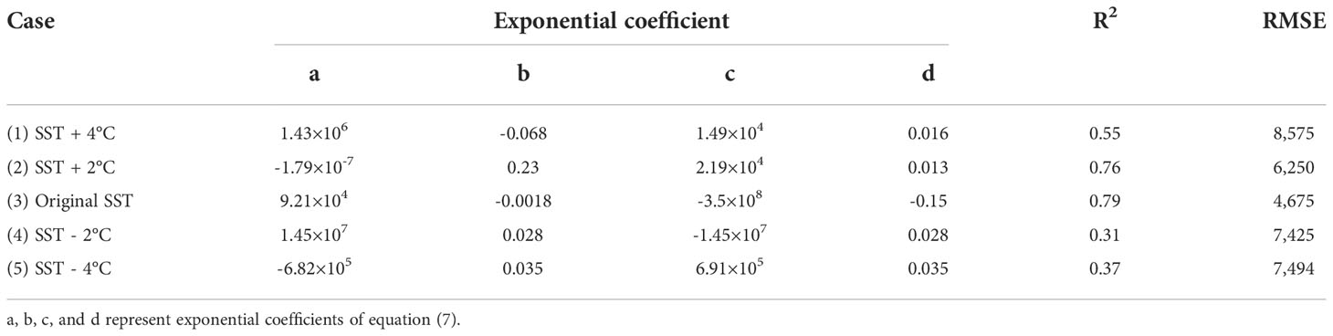
Table 4 Coefficient of the empirical polynomial regression for each case.
Discussions
Until now, previous studies have focused only on analyzing the tendency of Sargassum patches to move or the tendency of qualitative environmental factors such as mainly SST, ocean current, and wind data (Qi et al., 2017; Kim et al., 2019; Kwon et al., 2019). In fact, with these studies, it is difficult to quantitatively recognize environmental information on the location where the entire Sargassum patches exist in the East China Sea. Therefore, we quantitatively analyzed the relationship between environmental data and Sargassum distribution from 2015 to 2019 through a statistical approach, and generated Sargassum distribution estimation model through environmental data, and developed a machine learning model to estimate Sargassum distribution through environmental variables. In addition, it was possible to analyze the change in Sargassum distribution according to the adjustment of environmental variables. The following is a discussion of the results of this study.
Uncertainties of daily Sargassum map
The particle tracking model used for this study showed a good level with F-measure of 0.41. We attempted to compare the model used in Kwon et al. (2019) with the accuracy of our model. However, since the validation indexes of the two models are not the same, quantitative comparisons could not be performed. Alternatively, when comparing Sargassum distribution in 2017, we confirmed that Sargassum distribution in the ECS and YS by date were similar. Meanwhile, we analyzed the model accuracy in detail. Sargassum blooms began in February or March, and they were observed in GOCI image that lasted until April or May every year. Therefore, from the initial patch to the patch used for validation, the time difference ranged from 40 days in 2019 to 99 days in 2017. In 2017, the F-measure of Sargassum patch 13 days after the initial patch was 0.59, but the F-measure of the patch 99 days after from the initial patch was considerably reduced to 0.26. In addition, the F-measure and the sensitivity of patches observed in March in 2015 and 2019 were 0.43 and 0.55, respectively, while those of patches in May were 0.3 and 0.28, respectively. These results suggest that the accuracy of the daily Sargassum distribution decreased over time from that of the initial patch.
Several factors affect model performance. The uncertainty of the ground truth data extracted from GOCI may affect the performance. In 2016, we first found Sargassum patch on the coast of Zhejiang on March 2, using GOCI image. However, sea fog and cloud can detect only a partial distribution of Sargassum. As this model tracks the distribution of Sargassum based on initial patches, the inaccuracy of the initial patches affects the performance of the model. Sargassum pixels were extracted from GOCI dataset using the NDVI threshold. Moreover, as the extraction of pixels through a threshold does not consider various environmental factors such as submerged Sargassum, it often leads to overestimation or underestimation. Even the growth rate of Sargassum slows and sinks below seawater as it moves. Hence, when Sargassum patches approach the coast of the Korean Peninsula, complicating the ocean current system, they are extracted as satellite images, and the inaccuracy of extraction increases compared with that of the initial patches. Kwon et al. (2019) mentioned that because satellite images con not detect all patches, unmatched patches between synthetic particles and observed patches may appear. In addition, the particle tracking model used in this study failed to consider the physiological factors of Sargassum. For long-term particle tracking simulations, it is essential to consider the factors related to the growth and mortality of Sargassum (Putman et al., 2018; Wang et al., 2019). These limitations may reduce the accuracy of the model over time. Therefore, patches up to 50 days from the initial patch were used to develop a machine learning model that estimated Sargassum distribution from environmental variables.
Additional environmental variables
In addition to environmental variables used in this study, there are other environmental factors that affect Sargassum distribution. Qi et al. (2017) speculated that Photosynthetically active radiation (PAR) affect the occurrence of Sargassum bloom of the ECS. They argued that both SST and PAR are a major factor in determining the size of Sargassum patch. Wang et al. (2021) found that a higher temperature and lower light intensity exerted a negative influence on Sargassum through its cultivation. Zheng et al. (2022) reported that moderate light conditions can accelerate the growth and reproduction of Sargassum. Nutrients can affect Sargassum distribution. Bao et al. (2022) investigated the physiological responses of attached and pelagic Sargassum populations cultivated with different nutrient concentrations and PAR. They reported that nutrient restrictions and high PAR accelerate the senescence of pelagic populations while traveling on the sea surface from their point of origin. Qi et al. (2017) suggested that the early Sargassum on the Zhejiang coast may be the result of nutritional enrichment due to aquaculture. Due to the significant expansion of Prophyra aquaculture industry along the Zhejiang coast in recent years (China Fishery Statistical Yearbook (CFSY), 2009), it is possible that the nutrient-rich environment has been created due to increased fertilizer. The completion of the Three Gorges Dam (TGD) significantly impacted river discharge flowing into the ECS. Gong et al. (2006) suggested that the ECS ecosystem may respond sensitively to changes in the nutrient supply arising from the TGD project. It may cause changes in primary production, phytoplankton community structure, and biodiversity of the ECS (Wu et al., 2003; Fu et al., 2010). This change could sufficiently affect the prosperity and distribution of Sargassum patches in the ECS.
Various machine learning models
To confirm the ability of the machine learning model for future prediction, we used the pairs from 2015 to 2018 for training. Then, we tested the model using the pairs in 2019. As a result, the performance of BT-4 model showed reasonable level (sensitivity: 0.71, precision: 0.81, F-measure: 0.76, accuracy: 0.92). This suggested that our model can estimate Sargassum patches with a reasonable accuracy after 2020. Meanwhile, Sargassum generally moves along the ocean currents formed by wind and tends to grow or exterminate depending on the SST surrounding the flow. Therefore, the wind variable played a key role in the distribution of Sargassum. To recognize the impact of wind factors on Sargassum distribution, we trained and tested the BT-4 and BT-5 models by adding wsu and wsv variables. In BT-4 model, wsu and wsv variables were added to BT-2. For the BT-5 model, geographical and date variables were added to BT-4. The quantitative performance of both models showed good results, with the F-measure levels of 0.76 and 0.83, respectively. However, in the Sargassum map, the patches were distributed in a scattered form. It did not show a proper distribution compared with the ground truth map. These results show that wind data negatively affects the performance of the model, indicating that the distribution of wind stress values is not characterized by group, as shown in Figures 3G, H. This may be because our study focused on estimating daily Sargassum distribution using daily environmental data. As daily data cannot reflect the time lag of wind-driven seawater currents, their daily distribution cannot be properly estimated using daily wind data. We found that the wind trend from November to December of the previous year at the time of Sargassum occurrence determined the ocean current that moved Sargassum patch. This aspect is beyond the scope of this study, as we focused on instantaneous (up to one day) Sargassum distribution and not on the migration pattern of Sargassum. In addition, we trained machine learning models with various types of ensemble methods, including boosted trees, subspace discriminant, subspace k-nearest neighbor (KNN), and random undersampling boosting (RUSBoost) with decision tree using the training dataset used for the BT-3 model. Among these models, the RUSBoost model performed better than the other models. The RUSBoost model showed the highest sensitivity (0.92) and F-measure levels (0.59), while the boosted trees and KNN had the highest precision levels of 0.62 and 0.66, respectively. However, the subspace discriminant model exhibited the lowest F-measure (0.0001) and precision (0.0001) values. The learner type of RUSBoost is a decision tree, whereas those of the subspace discriminant are discriminant. The learner type of the BT-3 model that showed the best performance, was also a decision tree. These results suggest that our dataset shows the best performance when the ensemble method is a bag and the learner type is a decision tree.
Tolerable and favorable SST of Sargassum
Applying the BT-3 model, we simulated five cases with different SST variations to determine the effect of SST on Sargassum distribution. The cases in which the SST increased from the original tended to increase in area, showing a wider patch range than usual when reaching the Korean Peninsula. Conversely, the cases in which the SST decreased from the original showed a gradual increase in area and then decreased before reaching the Korean Peninsula. In fact, these results are related to tolerable SST associated with the growth or mortality of Sargassum. As mentioned, Sargassum grow in the SST range between 15 and 25 °C, while the optimal growth of adult Sargassum is in the range of 14−16 °C. In addition, our results showed that most of Sargassum group were distributed in the range of 14−18 °C. The average SST distributed by Sargassum patches was 16.04 °C. Considering the histogram in Sargassum group and daily Sargassum map, we determined tolerable SST to be 12−20 °C. When the SST was higher than the average SST, the increase rate of the area over time was higher. As shown in Figure 6, in general, a large amount of patches flow into the coast of the Korean Peninsula approximately 45 days after the initial patch is discovered off the coast of Zhejiang (yearday 106). Therefore, it may be inferred that if the SST increases in the ECS and the YS, the size of the patch flowing into the coast of Korean Peninsula will be larger than usual. In particular, for case (2), even when the patch reached the coast of the Korean Peninsula, the area continued to increase. It could be inferred that favorable SST for Sargassum was 18 °C. Conversely, when the SST was lower than the average SST, the area decreased from about 30 days after the initial patch. This means that the area of the patch decreases before it reaches Jeju Island, resulting in a lower probability of Sargassum existence around the Korean Peninsula. When the patches reached the Korean Peninsula, the largest difference in area between cases (1) and (5) was 44,583 km2 on April 17, 2016 (yearday 108).
Conclusion
In this study, we quantitatively analyzed the relationship between environmental variables and Sargassum distribution in the ECS and YS from 2015 to 2019 through statistical approach. Biotic and abiotic factors used for this study include SST, SS, SSH, rho, seawater current, and wind stress. Then, we developed a machine learning model for the estimation of Sargassum distribution through environmental variable. The developed model was applied to simulate Sargassum distribution by changing SST. The major results are as follows: (i) As a result of prioritizing environmental variables in a statistical approach, SST was the most important variable affecting Sargassum distribution in the ECS and YS. By confirming SSH, uo, and vo maps, we inferred that Sargassum patches cannot move southeast below 29°N because of the Kuroshio Current, (ii) the spatial distribution of Sargassum patches in the ECS and YS showed the most appropriate results when estimated through machine learning model derived from both geographical and physical information, and (iii) By simulating SST fluctuations, we identified the tolerable and favorable SST of Sargassum. These results will greatly help the understanding of the relationship between Sargassum distribution and environmental variables and also provide a method for the prevention and control of marine ecological disasters in Sargassum blooms.
Data availability statement
The original contributions presented in the study are included in the article/supplementary material. Further inquiries can be directed to the corresponding author.
Author contributions
Conceptualization: JS and Y-HJ. Data curation: JS, S-HK, and J-GC. Methodology: JS and Y-HJ. Formal analysis: JS. Writing-original draft: JS. Writing-review and editing: JS, S-HK, J-GC, B-KK, and Y-HJ. All authors contributed to the article and approved the submitted version.
Funding
This study was supported by the project titled “Development of technology using analysis of ocean satellite images” (20210046) funded by the Korea Institute of Marine Science & Technology Promotion (KIMST) and the National Research Foundation of Korea (NRF) grant funded by the Korea Government (MSIP) (NRF-2018R1A2B2006555).
Conflict of interest
The authors declare that the research was conducted in the absence of any commercial or financial relationships that could be construed as a potential conflict of interest.
Publisher’s note
All claims expressed in this article are solely those of the authors and do not necessarily represent those of their affiliated organizations, or those of the publisher, the editors and the reviewers. Any product that may be evaluated in this article, or claim that may be made by its manufacturer, is not guaranteed or endorsed by the publisher.
References
Bao M., Park J. S., Wu H., Lee H. J., Park S. R., Kim T. H., et al. (2022). A comparison of physiological responses between attached and pelagic populations of Sargassum horneri under nutrient and light limitation. Mar. Environ. Res. 173, 105544. doi: 10.1016/j.marenvres.2021.105544
Chen Y. L., Wan J. H., Zhang J., Ma Y. J., Wang L., Zhao J. H., et al. (2019). Spatial-temporal distribution of golden tide based on high-resolution satellite remote sensing in the south yellow Sea. J. Coast. Res. 90 (SI), 221–227. doi: 10.2112/SI90-027.1
China Fishery Statistical Yearbook (CFSY) (2009). Bureau of fisheries of the ministry of agriculture (Beijing, China : China Agriculture Publishing Press), 230pp.
Choi J. G., Jo Y. H., Moon I. J., Park J., Kim D. W., Lippmann T. C. (2018). Physical forces determine the annual bloom intensity of the giant jellyfish Nemopilema nomurai off the coast of Korea. Reg. Stud. Mar. Sci. 24, 55–65. doi: 10.1016/j.rsma.2018.07.003
Choi H. G., Lee K. H., Yoo H. I., Kang P. J., Kim Y. S., Nam K. W. (2007). “Physiological differences in the growth of sargassum horneri between the germling and adult stages,” in Nineteenth international seaweed symposium (Dordrecht: Springer), 279–285. doi: 10.1007/978-1-4020-9619-8_35
Das P., Lin A. T. S., Chen M. P. P., Miramontes E., Liu C. S., Huang N. W., et al. (2021). Deep-sea submarine erosion by the kuroshio current in the Manila accretionary prism, offshore southern Taiwan. Tectonophysics 807, 228813. doi: 10.1016/j.tecto.2021.228813
Ding C., Peng H. (2005). Minimum redundancy feature selection from microarray gene expression data. J. Bioinform. Comput. Biol. 3 (02), 185–205. doi: 10.1142/S0219720005001004
Fu B. J., Wu B. F., Lue Y. H., Xu Z. H., Cao J. H., Niu D., et al. (2010). Three gorges project: efforts and challenges for the environment. Prog. Phys. Geogr. 34 (6), 741–754. doi: 10.1177/0309133310370286
Gong G. C., Chang J., Chiang K. P., Hsiung T. M., Hung C. C., Duan S. W., et al. (2006). Reduction of primary production and changing of nutrient ratio in the East China Sea: Effect of the three gorges dam? Geophy.Res. Lett. 33 (7), L07610. doi: 10.1029/2006GL025800
Gounou A., Drévillion M., Clavier M. (2020). Product user manual for global ocean reanalysis products GLOBAL-REANALYSIS-PHY-001-031 (v1.1) (Toulouse, FRANCE: EU Copernicus Marine Service). Available at: https://catalogue.marine.copernicus.eu/documents/PUM/CMEMS-GLO-PUM-001-031.pdf.
Hsiung K. M., Kuo Y. C., Lin Y. T., Tseng Y. H., Han Y. S. (2022). North equatorial current and kuroshio velocity variations affect body length and distribution of the Japanese eel Anguilla japonica in Taiwan and Japan. Sci. Rep. 12 (1), 1–13. doi: 10.1038/s41598-022-06669-8
Hu D., Wu L., Cai W., Gupta A. S., Ganachaud A., Qiu B., et al. (2015). Pacific western boundary currents and their roles in climate. Nature 522 (7556), 299–308. doi: 10.1038/nature14504
Kang J., Na H. (2022). Long-term variability of the kuroshio shelf intrusion and its relationship to upper-ocean current and temperature variability in the East China Sea. Front. Mar. Sci. 9. doi: 10.3389/fmars.2022.812911
Kim K., Shin J., Kim K. Y., Ryu J. H. (2019). Long-term trend of green and golden tides in the Eastern yellow Sea. J. Coast. Res. 90 (SI), 317–323. doi: 10.2112/SI90-040.1
Komatsu T., Matsunaga D., Mikami A., Sagawa T., Boisnier E., Tatsukawa K., et al. (2007a). “Abundance of drifting seaweeds in eastern East China Sea,” in Nineteenth international seaweed symposium (Dordrecht: Springer), 351–359. doi: 10.1007/978-1-4020-9619-8_44
Komatsu T., Tatsukawa K., Filippi J. B., Sagawa T., Matsunaga D., Mikami A., et al. (2007b). Distribution of drifting seaweeds in eastern East China Sea. J. Mar. Syst. 67 (3-4), 245–252. doi: 10.1016/j.jmarsys.2006.05.018
Kwon K., Choi B. J., Kim K. Y., Kim K. (2019). Tracing the trajectory of pelagic Sargassum using satellite monitoring and Lagrangian transport simulations in the East China Sea and yellow Sea. Algae 34 (4), 315–326. doi: 10.4490/algae.2019.34.12.11
Lee S. Y. (2018). Analysis of the physical factors affecting the inflow of sargassum horneri into adjacent seas of jeju island using particle tracking experiment (Jeju, South Korea: Doctoral dissertation, Jeju National University).
Lin S. M., Huang R., Ogawa H., Liu L. C., Wang Y. C., Chiou Y. (2017). Assessment of germling ability of the introduced marine brown alga, Sargassum horneri, in northern Taiwan. J. Appl. Phys. 29 (5), 2641–2649. doi: 10.1007/s10811-017-1088-4
Liu F., Liu X., Wang Y., Jin Z., Moejes F. W., Sun S. (2018). Insights on the Sargassum horneri golden tides in the yellow Sea inferred from morphological and molecular data. Limnol. Oceanog. 63 (4), 1762–1773. doi: 10.1002/lno.10806
McDougall T. J., Barker P. M. (2011). Getting started with TEOS-10 and the Gibbs seawater (GSW) oceanographic toolbox. Scor/Iapso WG 127, 1–28.
Mikami A., Komatsu T., Aoki M., Yokohama Y. (2006). Seasonal changes in growth and photosynthesis-light curves of Sargassum horneri (Fucales, phaeophyta) in oura bay on the pacific coast of central Honshu, Japan. Mer 44 (3/4), 109–118.
Mizuno S., Ajisaka T., Lahbib S., Kokubu Y., Alabsi M. N., Komatsu T. (2014). Spatial distributions of floating seaweeds in the East China Sea from late winter to early spring. J. Appl. Phycol. 26 (2), 1159–1167. doi: 10.1007/s10811-013-0139-8
Pang S. J., Liu F., Shan T. F., Gao S. Q., Zhang Z. H. (2009). Cultivation of the brown alga Sargassum horneri: sexual reproduction and seedling production in tank culture under reduced solar irradiance in ambient temperature. J. Appl. Phycol. 21 (4), 413–422. doi: 10.1007/s10811-008-9386-5
Press Release Provided by Yonhapnews. Available at: https://www.yna.co.kr/view/AKR20210217152600054 (Accessed July 28, 2022).
Putman N. F., Goni G. J., Gramer L. J., Hu C., Johns E. M., Trinanes J., et al. (2018). Simulating transport pathways of pelagic Sargassum from the equatorial Atlantic into the Caribbean Sea. Progr. Oceanogr. 165, 205–214. doi: 10.1016/j.pocean.2018.06.009
Qi L., Hu C., Wang M., Shang S., Wilson C. (2017). Floating algae blooms in the East China Sea. Geophys. Res. Lett. 44 (22), 11–501. doi: 10.1002/2017GL075525
Rouse J. W., Haas R. H., Deering D. W., Schell J. A., Harlan J. C. (1974). Monitoring the vernal advancement and retrogradation (green wave effect) of natural vegetation. NASA/GSFC Type III Final Rep. Greenbelt Md 371.
Samek W., Wiegand T., Müller K. R. (2017). Explainable artificial intelligence: Understanding, visualizing and interpreting deep learning models. CoRR 08296, 1–6. doi: 10.48550/arXiv.1708.08296
Trenberth K. E., Large W. G., Olson J. G. (1990). The mean annual cycle in global ocean wind stress. J. Phys. Oceanogr. 20 (11), 1742–1760. doi: 10.1175/1520-0485(1990)020<1742:TMACIG>2.0.CO;2
Wang M., Hu C., Barnes B. B., Mitchum G., Lapointe B., Montoya J. P. (2019). The great Atlantic Sargassum belt. Sci. 365 (6448), 83–87. doi: 10.1126/science.aaw7912
Wang Y., Zhong Z., Qin S., Li J., Li J., Liu Z. (2021). Effects of temperature and light on growth rate and photosynthetic characteristics of Sargassum horneri. J. Ocean Uni. China 20 (1), 101–110. doi: 10.1007/s11802-021-4507-8
Welander P. (1957). Wind action on a shallow sea: some generalizations of ekman's theory. Tellus 9 (1), 45–52. doi: 10.1111/j.2153-3490.1957.tb01852.x
Wojtas M., Chen K. (2020). Feature importance ranking for deep learning. Adv. Neural Inf. Process. Syst. 33, 5105–5114.
Wu H., Feng J., Li X., Zhao C., Liu Y., Yu J., et al. (2019). Effects of increased CO2 and temperature on the physiological characteristics of the golden tide blooming macroalgae Sargassum horneri in the yellow Sea, China. Mar. pollut. Bull. 146, 639–644. doi: 10.1016/j.marpolbul.2019.07.025
Wu J., Huang J., Han X., Xie Z., Gao X. (2003). Three-gorges dam–experiment in habitat fragmentation? Science 300 (5623), 1239–1240. doi: 10.1126/science.1083312
Xing Q., Wu L., Tian L., Cui T., Li L., Kong F., et al. (2018). Remote sensing of early-stage green tide in the yellow Sea for floating-macroalgae collecting campaign. Mar. pollut. Bull. 133, 150–156. doi: 10.1016/j.marpolbul.2018.05.035
Xu M., Sakamoto S., Komatsu T. (2016). Attachment strength of the subtidal seaweed Sargassum horneri (Turner) c. agardh varies among development stages and depths. J. Appl. Phycol. 28 (6), 3679–3687. doi: 10.1007/s10811-016-0869-5
Yang S. L., Milliman J. D., Li P., Xu K. (2011). 50,000 dams later: erosion of the Yangtze river and its delta. Glob. Planet. Change 75 (1-2), 14–20. doi: 10.1016/j.gloplacha.2010.09.006
Yuan C., Xiao J., Zhang X., Fu M., Wang Z. (2022). Two drifting paths of Sargassum bloom in the yellow Sea and East China Sea during 2019–2020. Acta Oceanologica Sin. 41 (6), 78–87. doi: 10.1007/s13131-021-1894-z
Yuan C. Y., Yang S., Wang Y., Cui Q. M. (2014). Effect of temperature on the growth and biochemical composition of sargassum muticum.Adv. Mater. Res., 989. 747–750). doi: 10.4028/www.scientific.net/AMR.989-994.747
Yun C. X. (2004). Recent evolution of the Yangtze estuary and its mechanisms Vol. 2004 (Beijing: China Ocean Press).
Zhang J., Ding X., Zhuang M., Wang S., Chen L., Shen H., et al. (2019). An increase in new Sargassum (Phaeophyceae) blooms along the coast of the East China Sea and yellow Sea. Phycologia 58 (4), 374–381. doi: 10.1080/00318884.2019.1585722
Zheng L., Wu M., Zhou M., Zhao L. (2022). Spatiotemporal distribution and influencing factors of Ulva prolifera and Sargassum and their coexistence in the south yellow Sea, China. J. Oceanol. Limnol. 40 (3), 1070–1084. doi: 10.1007/s00343-021-1040-y
Keywords: Sargassum horneri, GOCI, particle-tracking experiment, machine learning, feature importance ranking
Citation: Shin J, Choi J-G, Kim S-H, Khim B-K and Jo Y-H (2022) Environmental variables affecting Sargassum distribution in the East China Sea and the Yellow Sea. Front. Mar. Sci. 9:1055339. doi: 10.3389/fmars.2022.1055339
Received: 27 September 2022; Accepted: 28 November 2022;
Published: 08 December 2022.
Edited by:
Zi-Min Hu, Yantai University, ChinaCopyright © 2022 Shin, Choi, Kim, Khim and Jo. This is an open-access article distributed under the terms of the Creative Commons Attribution License (CC BY). The use, distribution or reproduction in other forums is permitted, provided the original author(s) and the copyright owner(s) are credited and that the original publication in this journal is cited, in accordance with accepted academic practice. No use, distribution or reproduction is permitted which does not comply with these terms.
*Correspondence: Young-Heon Jo, am95b3VuZ0BwdXNhbi5hYy5rcg==