A dual stream hierarchical transformer for starvation grading of golden pomfret in marine aquaculture

Introduction: Fish starvation grading can provide feeding information for aquaculture, reducing the cost of lures and helping to promote the unmanned and intelligent process of offshore aquaculture.

Methods: In this study, we used golden pompano as the experimental object to address the fish starvation grading problem in the marine culture vessel environment, and proposed the dual stream hierarchical transformer to provide additional temporal information for the starvation grading task, which improved the grading accuracy. We first built a dual stream dataset with both spatial and temporal channel, and divided the fish school starvation status into five levels (very bloated, a little bloated, modest, a little starving, very starving) according to the feeding time and experience. Based on the marine image characteristics, we proposed a dual stream hierarchical transformer with hierarchical convolutional network, composite fusion convolution and transformer.

Results and discussion: We finally evaluated the efficacy of the model based on qualitative and quantitative analyses, revealing that the proposed dual stream hierarchical transformer achieved the state-of-the-art starvation grading performance with a test accuracy of 98.05%. Our model outperformed other mainstream models, including VGG, ResNet, attentionbased model and other fish status grading related model. Field tests on the vessel further suggested that the model can be applied to the mariculture environment of golden pomfret.

Introduction

Feeding is an essential step in the aquaculture procedure. The effectiveness of the feeding plan not only has an impact on fish growth directly, but also has influence on costs and environmental contamination when lures are wasted. The cost of lures makes up about 30% of the entire investment in aquaculture (Hossain et al., 2022), and Lin’s environmental study report noted that uneaten fish food would lead to a number of environmental issues, including the production of greenhouse gases (Lin and Lin, 2022). According to experimental data (Jothiswaran et al., 2020), using the AI-controlled machine to feed fish and dynamically modify feeding strategies based on fish status can prevent at least 30% of bait waste. In order to minimize economic losses and pollution, it is crucial to optimize fish condition-based feeding techniques to improve bait waste using AI techniques.

Inspired by deep learning used in image recognition tasks, fish researchers have used these methods to analyze fish behavior. There are individual- and school-based identifying and analyzing approaches. Individual-based methods monitor the individual fish in a clear laboratory environment and use the tracked trajectory for identification, such as swimming speed, direction, acceleration, and body curvature (Jonas et al., 2017). As a result, the validity of the tracked trajectory and the accuracy of fish identification are the two key determinants of study for this type of study.

In real mariculture, problems occur when fish were overlap in the image and when the camera could not capture the whole environment. This made it challenging for the trajectory tracking and fish identification. To avoid the requirement to blindly monitor individual fish, the status or behaviors of the fish school may be deduced from the fish visible in the image using the fish school analysis technique. These techniques are known as school-based techniques (Måløya et al., 2019). The following is an overview of school-based approaches to fish behavior or state recognition: The fish school is first mapped in grayscale using the background and foreground segmentation technique (Ye et al., 2016). The fish’s overall optical flow images, such as swimming speed and acceleration, are then obtained by using the grayscale map as a foundation (Zhao et al., 2018). Finally, a prediction network is used for recognition (Zhou et al., 2017). About the fish school status grading, a 5-layers CNN was used to classify the intensity of fish school feeding (Zhou et al., 2019). DSRN (Måløya et al., 2019) used 3D residual convolution and LSTM to classify salmon feeding or non-feeding states. On the other hand, DAN-EfficientNet-B2 (Yang et al., 2021) used an attention-based approach to classify the foraging behavior of Oplegnathus punctatus into five categories. DADSN (Zheng et al., 2022) used the combination of CNN and Transformer for the grading of fish starvation.

Convolutional Neural Network (CNN, Lecun et al., 1998) is proposed and then a lot of CNN-based model sprang up. Krizhevsky et al. proposed a five-layer CNN for image classification and won the ILSVRC competition (Krizhevsky et al., 2012). In the following time, CNN became a hot research topic and developed rapidly. Many classical models were created, such as GoogLeNet (Szegedy et al., 2015) and ResNet (He et al., 2016).

Nowadays, numerous experiments have shown that CNN has the following limitations: First, CNN uses local receptive fields for feature capture and thus cannot directly build the global model; Second, weights learned by CNN are stationary at the time of inference, which makes them unadaptable for various inputs (Raghu et al., 2021). Attention models are a popular area of research in current image recognition studies, with flexible modelling capabilities for Regions of Interest (RoI) that can be used for single image or video recognition. In particular, researchers (Fu et al., 2019) used attention models to study the feeding state of fish in a single image, but unfortunately, this approach was only tested in their laboratory dataset and was not extended to real farming.

In this paper, daily data of fish in commercial aquaculture vessels of golden pomfret was collected. Then a Dual Stream Hierarchical Transformer (DSHT) is proposed. First, a Hierarchical Convolutional Network (HCN) was used as the backbone network to extract mariculture image features. Second, we built spatial and temporal channels, called dual stream structure, to make the input data contain richer information. Among them, the spatial features mainly express the distribution, number, and texture of fish; the temporal features mainly represent the movement changes in time series, such as the swimming speed and acceleration of fish. Finally, the spatial and temporal information is fused and filtered using a Composite Fusion Network (CFN). The method achieved 98.05% accuracy and provided valuable feeding control information for intelligent feeding.

Proposed model

Hierarchical convolutional network

Similar to the process of human vision, CNN learn the ability of feature extraction from surface to deep information. The shallow convolutional layers focus on the detailed information of the object within the image, while the deep convolutional layers focus on the abstract semantic information. The features produced form different depth layers require different visual perception fields. Detailed information such as graphic contours requires a smaller field of view to find these details, so small convolutional kernels are more suitable, while abstract semantic information requires larger convolutional kernels to detect. Therefore, we propose a Hierarchical Convolutional Network (HCN), which divides the features of an image into three categories: shallow, medium, and deep, and uses different convolutional kernels for each layer. As shown in Figure 1D. The HCN first dimensionally expands the input image. Then three types of CNN with different kernel sizes are used to obtain the hierarchical features. Finally, the obtained features are further refined by a compression network, respectively. In this paper, Gaussian Error Linear Units (GELU, Hendrycks and Gimpel, 2016) is used as the activation function. The formula is expressed as follows:

$\begin{array}{ll}{\mathbf{C}}_{\mathbf{i}}(\mathbf{X})\mathbf{=}\mathbf{G}\mathbf{E}\mathbf{L}\mathbf{U}({\mathbf{W}}_{\mathbf{i}}\mathbf{\ast }\mathbf{X}\mathbf{+}\mathbf{b})\mathbf{,}\mathbf{i}\mathbf{=}\mathbf{1}\mathbf{,}\mathbf{2}\mathbf{,}\mathbf{3}& (1)\end{array}$

FIGURE 1

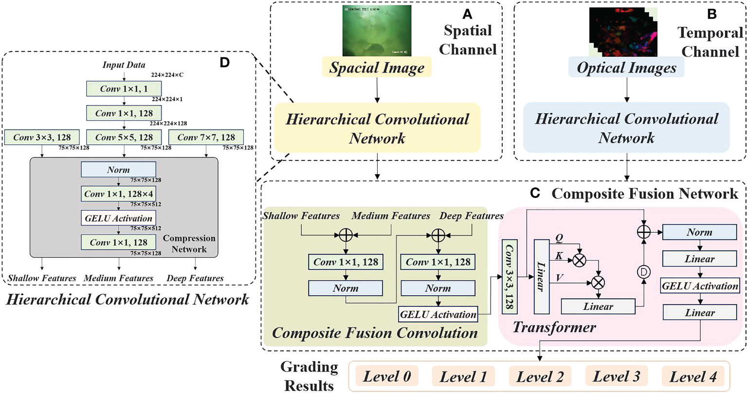
Figure 1 The Architecture and Stages of Dual Stream Hierarchical Transformer (DSHT). (A) is the spatial channel, and (D) is the HCN which is used to process the input and output three hierarchical feature blocks. (B) is the temporal channel which uses the similar approach with spatial channel. (C) is CFN, which is made up of CFC and Transformer.

Where X is the input, C_i is the out, W_i is the weight matrix, b is the bias, the symbol * denotes the convolution operation, and GELU(x) is the activation function:

$\begin{array}{ll}\mathbf{G}\mathbf{E}\mathbf{L}\mathbf{U}(\mathbf{x})\mathbf{=}\mathbf{x}\mathbf{P}(\mathbf{X}\mathbf{\le }\mathbf{x})\mathbf{=}\mathbf{x}\mathbf{N}(\mathbf{\mu }\mathbf{,}\mathbf{\sigma })\mathbf{=}\mathbf{0.5}\mathbf{x}(\mathbf{1}\mathbf{+}\mathbf{t}\mathbf{a}\mathbf{n}\mathbf{h}[\sqrt{\mathbf{2}/\mathbf{\pi })}(\mathbf{x}\mathbf{+}\mathbf{0.044715}{\mathbf{x}}^{\mathbf{3}})])& (2)\end{array}$

where N(µσ) is the positive-terrestrial distribution.

Dual stream structure

If only one image is used as the input, the neural network will lack the temporal information, which are pretty importance features for fish school behavior, such as speed and direction. Since the difference between two adjacent images is not obvious, there would be a lot of redundant information if we used consecutive images as input. In this paper, optical flow images were used to represent temporal information. The architecture is referred to as a dual stream structure, where the input of the spatial channel is a spatial image and the inputs of the temporal channel are 20 continuous optical flow images. The optical flow image is an image that records the change of light over time, and it uses the pixels change of neighboring spatial images as the basis to calculate the of motion information (Ranjan and Black, 2017). Assume that the pixel value of (x, y) at time t can be represented by function I(x, y, t), the pixel in the frame t + 1 is generated by the pixel I(x, y, t) that has moved a distance (dx, dy) in time dt, so we have:

$\begin{array}{ll}\mathbf{I}(\mathbf{x}\mathbf{,}\mathbf{y}\mathbf{,}\mathbf{t})\mathbf{=}\mathbf{I}(\mathbf{x}\mathbf{+}\mathbf{d}\mathbf{x}\mathbf{,}\mathbf{y}\mathbf{+}\mathbf{d}\mathbf{y}\mathbf{,}\mathbf{t}\mathbf{+}\mathbf{d}\mathbf{t})& (3)\end{array}$

If the parameters dx, dy, and dt are small enough, the approximation equation can be obtained by neglecting higher-order infinitesimals:

$\begin{array}{ll}\mathbf{I}(\mathbf{x}\mathbf{+}\mathbf{d}\mathbf{x}\mathbf{,}\mathbf{y}\mathbf{+}\mathbf{d}\mathbf{y}\mathbf{,}\mathbf{t}\mathbf{+}\mathbf{d}\mathbf{t})\mathbf{=}\mathbf{I}(\mathbf{x}\mathbf{,}\mathbf{y}\mathbf{,}\mathbf{t})\mathbf{+}{\mathbf{I}}_{\mathbf{x}}\mathbf{u}\mathbf{d}\mathbf{t}\mathbf{+}{\mathbf{I}}_{\mathbf{y}}\mathbf{v}\mathbf{d}\mathbf{t}\mathbf{+}{\mathbf{I}}_{\mathbf{t}}\mathbf{d}\mathbf{t}& (4)\end{array}$

Where I_x is the bias of the pixel value against x, I_yis the bias of the pixel value against y, I_t is the bias of the grey value against t, u = dx/dt and v = dy/dt represents the instantaneous velocity of the pixel in the x direction and ydirection respectively. Combining the Eq.(3) and Eq.(4), we can obtain the constraint equation:

$\begin{array}{ll}{\mathbf{I}}_{\mathbf{x}}\mathbf{u}\mathbf{+}{\mathbf{I}}_{\mathbf{y}}\mathbf{v}\mathbf{+}{\mathbf{I}}_{\mathbf{t}}\mathbf{=}\mathbf{0}& (5)\end{array}$

By solving the above equations for the variables u and v , we can obtain temporal information about the movement of the pixels within the image. In this paper, we adopt the solution proposed by Bruce (Lucas, 1985). The visualization of the above calculation results is the optical flow diagram dataset mentioned in this paper.

Feature fusion and transformer

In cognitive science, humans selectively focus on a portion of information due to the bottlenecks in information processing. The transformer is an attention model which imitate the process of human visual observation (Maaz et al., 2022). In this paper, the transformer is used to better perceive the important regions of features between the spatial and temporal channels.

As shown in Figure 1C, the Composite Fusion Network (CFN) consists of two parts: the Composite Fusion Convolution (CFC) and the Transformer. First, the HCN outputs of C₁(X) (shallow block) and C₂(X) (medium block) are added, then the features are encoded by a convolutional layer. Then they are added with C₃(X) (deep block) and encoded by another convolutional layer.

$\begin{array}{ll}\mathbf{C}\mathbf{F}\mathbf{C}(\mathbf{X})\mathbf{=}\mathbf{G}\mathbf{R}\mathbf{L}\mathbf{U}({\mathbf{W}}_{\mathbf{2}}\mathbf{\ast }({\mathbf{W}}_{\mathbf{1}}\mathbf{\ast }({\mathbf{C}}_{\mathbf{1}}(\mathbf{X})\mathbf{+}{\mathbf{C}}_{\mathbf{2}}(\mathbf{X}))\mathbf{+}{\mathbf{C}}_{\mathbf{3}}(\mathbf{X})))& (6)\end{array}$

W₁ and W₂ are the weight matrix of CFC, C₁(X), C₂(X), and C₃(X) are the output of HCN.

The input of Transformer is the outputs of CFC, which are spread into a two-dimensional matrix. In Transformer, two matrices E and E_pos are also created, where E denotes the weight of the transformer values, indicating which features need to be focused on. E_pos is the position encoding, and used to represent the position relationship between features. The expression formula is as follows:

$\begin{array}{ll}{\mathbf{z}}_{\mathbf{0}}\mathbf{=}[\mathbf{X}{\mathbf{E}}_{\mathbf{1}}\mathbf{;}\mathbf{X}{\mathbf{E}}_{\mathbf{2}}\mathbf{;}\mathbf{X}{\mathbf{E}}_{\mathbf{3}}]\mathbf{+}{\mathbf{E}}_{\mathbf{p}\mathbf{o}\mathbf{s}}& (7)\end{array}$

Where z₀ denotes the initial result. E₁, E₂ and E₃ are the individual dimension of the weight matrix E. XE₁, XE₂, and XE₃ are the intermediate variables Q, K and V, respectively.

The Q, K and V are transposed and multiplied, and the softmax results are summed with the input to obtain the intermediate results for the current layer.

$\begin{array}{ll}\mathbf{z}{\mathbf{\text{'}}}_{\mathbf{l}}\mathbf{=}\mathbf{s}\mathbf{o}\mathbf{f}\mathbf{t}\mathbf{m}\mathbf{a}\mathbf{x}\left(\mathbf{\alpha }(\mathbf{Q}\mathbf{·}{\mathbf{K}}^{\mathbf{T}})\right)·\mathbf{V}\mathbf{+}{\mathbf{z}}_{\mathbf{l}-\mathbf{1}}\mathbf{,}\mathbf{l}\mathbf{=}\mathbf{1}\mathbf{,}\mathbf{·}\mathbf{·}\mathbf{·},\mathbf{L}& (8)\end{array}$

Where z’_l is the attention results. z_l–1 is the output of the previous attention. K^T is the transpose of the variable K, the symbol is matrix multiplication, α is the normalization factor, and $softmax(z_i)=\frac{e^{z_i}}{{\displaystyle {\sum }_{j=1}^J{e}^{z_j}}}$ is the activation function.

The z_l is the final output which obtained by normalizing, bottleneck compressing and add with the attention results z’_l.

$\begin{array}{ll}{\mathbf{z}}_{\mathbf{l}}\mathbf{=}\mathbf{M}\mathbf{L}\mathbf{P}(\mathbf{L}\mathbf{N}(\mathbf{n}\mathbf{o}\mathbf{r}\mathbf{m}\mathbf{z}(\mathbf{z}{\mathbf{\text{'}}}_{\mathbf{l}})\mathbf{,}\mathbf{\gamma }\mathbf{d}\mathbf{i}\mathbf{m}))\mathbf{+}\mathbf{z}{\mathbf{\text{'}}}_{\mathbf{l}}\mathbf{,}\mathbf{l}\mathbf{=}\mathbf{1}\mathbf{,}\mathbf{·}\mathbf{·}\mathbf{·}\mathbf{,}\mathbf{L}& (9)\end{array}$

Where norm(z’_l) represents normalize the attention results z’_l, LN(x) is compress its dimension to the γ times, which is taken as 0.6 in this paper. MLP(x) are dropout, activation, and restore features to the original dimension.

Dual stream hierarchical transformer

The Dual Stream Hierarchical Transformer (DSHT) proposed in this paper is shown in Figure 1. Fist, a spatial image is fed into the spatial channel and extracted by HCN shown in Figure 1D to obtain three hierarchical feature blocks (shallow features, medium features, and deep features). Then, the hierarchical feature blocks are fused by CFC mentioned in Figure 1C to produce the spatial features. For the temporal channel Figure 1B, we take 20 consecutive optical flow images as input and process them with another HCN and CFC like the spatial channel to produce the temporal features. Further, connecting the spatial features and temporal features by the transformer shown in Figure 1C to eliminate useless or duplicate features. Finally, the output of the transformer is converted into a 5-dimensional vector by full concatenation, which represents the grading results of the input samples.

Experimental details

Environment and data collection

We equipped an underwater camera (GW-10, Hikvision) on the aquaculture vessel to record the pomfret video of the starvation status (The yellow box in Figure 2B. As shown in Figure 2A, the vessel has five aquaculture cabins, each of which is a 4×4×3 m³ rectangle. The farming vessel carries out aquaculture operations in the Beihai, Guangxi Province, about 15 nautical miles from the coastline. The suction pump is used to extract seawater for breeding. Four inlets are configured on each of the four sides of a cabin (The red box in Figure 2B). The bottom of a cabin has a drainage port (The blue box in Figure 2B). It is also equipped with the equipment needed to maintain a suitable environment for aquaculture.

FIGURE 2

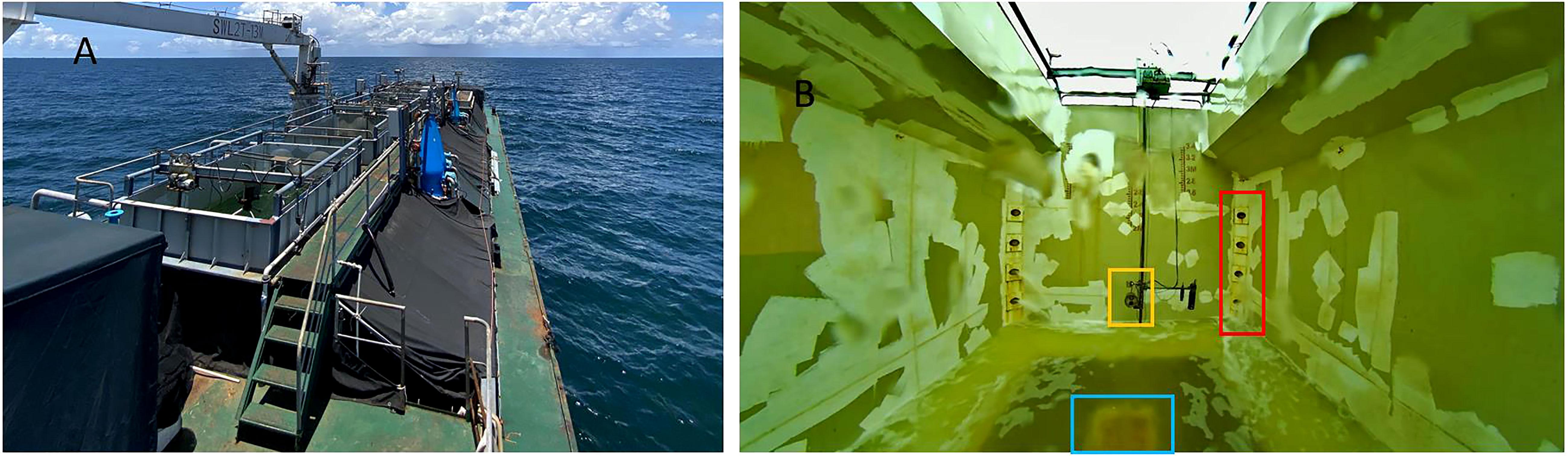
Figure 2 (A) is the vessels enviroment. (B) is the aquacultural enviroment, and the yellow box, red box and blue box are underwater camera, inlets and outlet, respectively.

In this paper, fingerlings provided by Guangxi Jingong Marine Technology Co., Ltd., Beihai, China. A breeding cabins has 800 fish, each weighing about 500 g. Feeding was carried out daily in the morning (6:00 - 8:00 am), noon (11:00 am - 13:00 pm), and evening (5:00 - 7:00 pm). Feeding time lasts approximately 10 minutes. the weight of the lures is decided according to the weather and environment. The hunger levels were divided into a total of 5 levels, as shown in Table 1.

TABLE 1

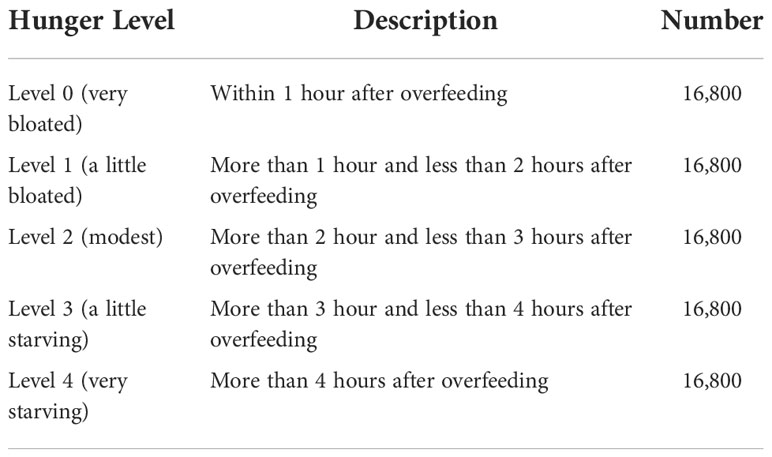
Table 1 The Grading Standards.

Dataset creation

According to the aquaculture data recorded by the breeders, we labelled the fish starvation levels from the videos captured by the underwater camera. A total of 84,000 samples were divided, each containing one spatial image and twenty optical flow images. The training set, validation set, and test set were divided in the ratio of 6:2:2, and the number of samples in each level was kept consistent. As shown in Table 2.

TABLE 2

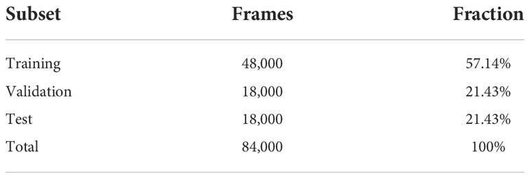
Table 2 The distribution of the Dataset.

Metrics

In this paper, three metrics, accuracy, precision, and F1-score, are used to evaluate the model performance. Accuracy indicates whether the model can accurately grade the starvation level of fish. Precision is used to determine how difficult it is to correctly grade samples in that level, and F1-score is used as a comprehensive evaluation index of model performance. It is worth noting that the recall rate is not used in this paper. Since we keep the sample number of each category consistent in order to ensure that training can proceed smoothly. The recall rate and accuracy rate are the same.

$\begin{array}{ll}\mathbf{A}\mathbf{c}\mathbf{c}\mathbf{u}\mathbf{r}\mathbf{a}\mathbf{c}\mathbf{y}\mathbf{=}\frac{\mathbf{T}\mathbf{P}\mathbf{+}\mathbf{T}\mathbf{N}}{\mathbf{T}\mathbf{P}\mathbf{+}\mathbf{F}\mathbf{N}\mathbf{+}\mathbf{F}\mathbf{P}\mathbf{+}\mathbf{F}\mathbf{N}}\times \mathbf{100}\%& (10)\end{array}$

$\begin{array}{ll}\mathbf{P}\mathbf{r}\mathbf{e}\mathbf{c}\mathbf{i}\mathbf{s}\mathbf{i}\mathbf{o}\mathbf{n}\mathbf{=}\frac{\mathbf{T}\mathbf{P}}{\mathbf{T}\mathbf{P}\mathbf{+}\mathbf{F}\mathbf{P}}\times \mathbf{100}\%& (11)\end{array}$

$\begin{array}{ll}\mathbf{F}\mathbf{1}\mathbf{s}\mathbf{c}\mathbf{o}\mathbf{r}\mathbf{e}=\frac{\mathbf{2}\mathbf{T}\mathbf{P}}{\mathbf{2}\mathbf{T}\mathbf{P}\mathbf{+}\mathbf{F}\mathbf{P}\mathbf{+}\mathbf{F}\mathbf{N}}\times \mathbf{100}\%& (12)\end{array}$

TP is the number of samples labelled with the positive class and correctly classified by the model; TN is the number of samples labelled with the negative class and correctly classified by the model; FP is the number of samples labelled as negative but incorrectly classified by the model; and FN is the number of samples labelled as positive but incorrectly classified by the model.

Experimental setting

The models mentioned in this paper are run on a GPU server in V100. The Python and Pytorch architectures are used. Cross entropy is used as the loss function, the batch size is 32, and 30 rounds are trained. The dynamic learning rate is 0.002 and the dropout rate is 0.01.

Results

Ablation experiments

As shown in Table 3, ablation experiments were designed to verify the feasibility and usefulness of the modules proposed in DSHT. Also, we try to connect these modules in various ways with different input data. There are three type date of the input: only optical flow images (OP), only spatial images (SP) and dual stream images (DS, both of spatial and optical flow images). We test three basic modules in DSHT: Hierarchical Convolutional Network (HCN), Composite Fusion Convolution (CFC) and Transformer, and Transformer have two patterns: piecemeal Transformer and global Transformer. If the feature blocks of HCN are connected before Transformer, the pattern is called global Transformer, and opposite is called piecemeal Transformer. For example, in Table 3, The HCN (OP) model using optical flow images as inputs and only a HCN module to grade the starvation of fish school. On the contrary, the model of HCN + CFC + global Transformer (DS) (DSHT), is the proposed model in this paper.

TABLE 3

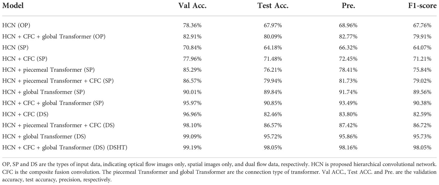
Table 3 The Grading Standards.

As shown in Table 3, the HCN (OP) and HCN (SP) are the baseline models, the accuracy of test dataset reaches 67.97% and 64.18%, respectively. By adding the CFC and Transformer to the baseline model, all of the indexes have been improved. The HCN + CFC (SP) model is built by adding the CFC based on HCN, which achieve 71.48%, 72.45% and 71.21% of test accuracy, precision and F1-score. The HCN + piecemeal Transformer (SP) and the HCN + global Transformer (SP) are built by applying the Transformer with different forms, and their test accuracy are 76.21% and 89.84%, respectively. Further, comparing with the single spatial or temporal channel, the performances of dual-stream structure with same methods are more remarkable. The test accuracy of HCN + CFC (DS) model and HCN + global Transformer (DS) model are 82.46% and 95.72%, respectively. If both HCN, CFC and Transformer are used, the model will show even better grading results, e.g. DSHT, which has the best performance with the accuracy, precision and F1-sorce of 98.05%, 98.16% and 98.05%, respectively. Figure 3 shows the accuracy curves of the ablation models in the validation set during the training process. Figure 4 is the visualization of models’ output features mentioned in Table 3.

FIGURE 3

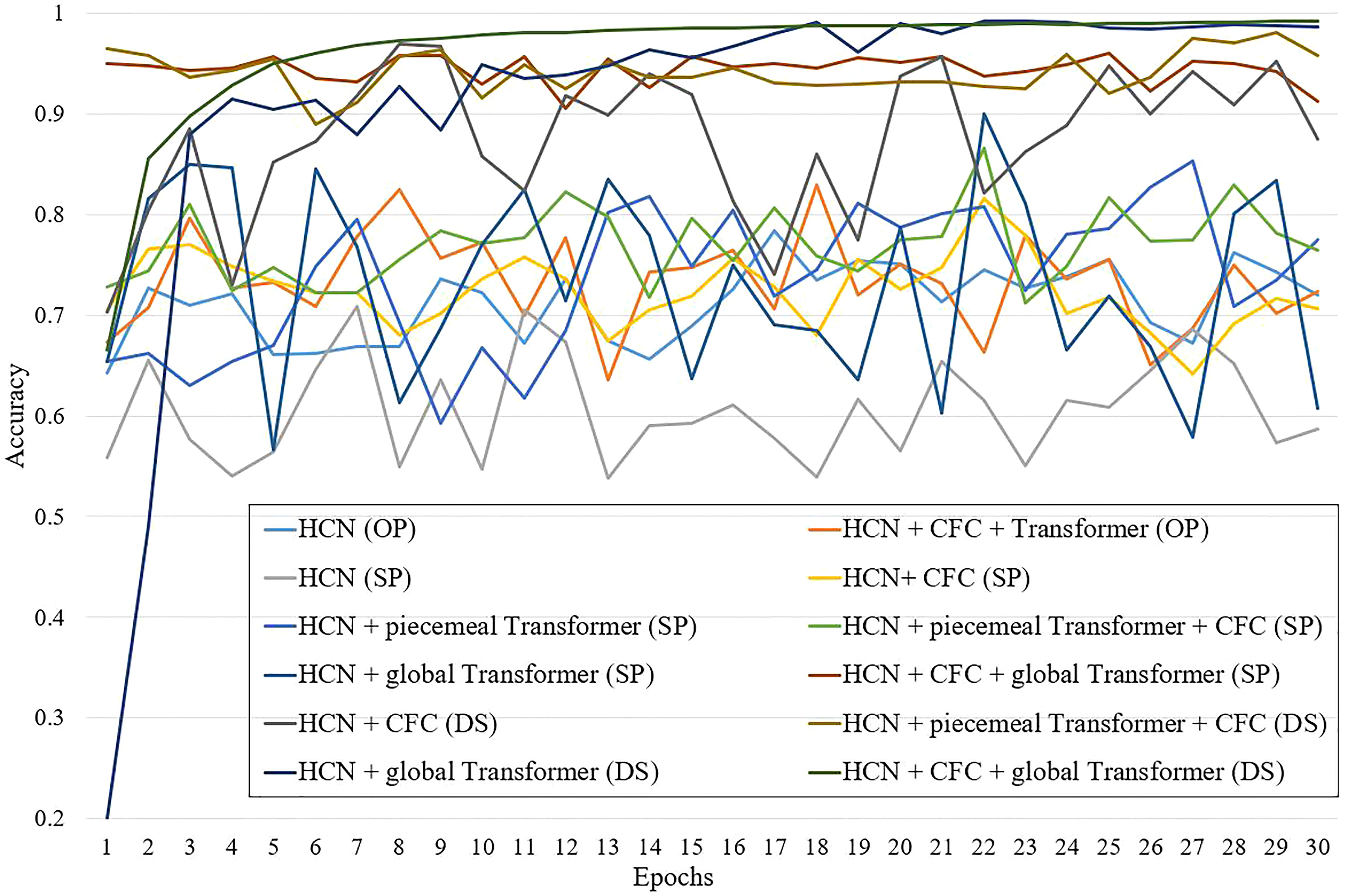
Figure 3 Validation Accuracy Curves of Ablation Models.

FIGURE 4

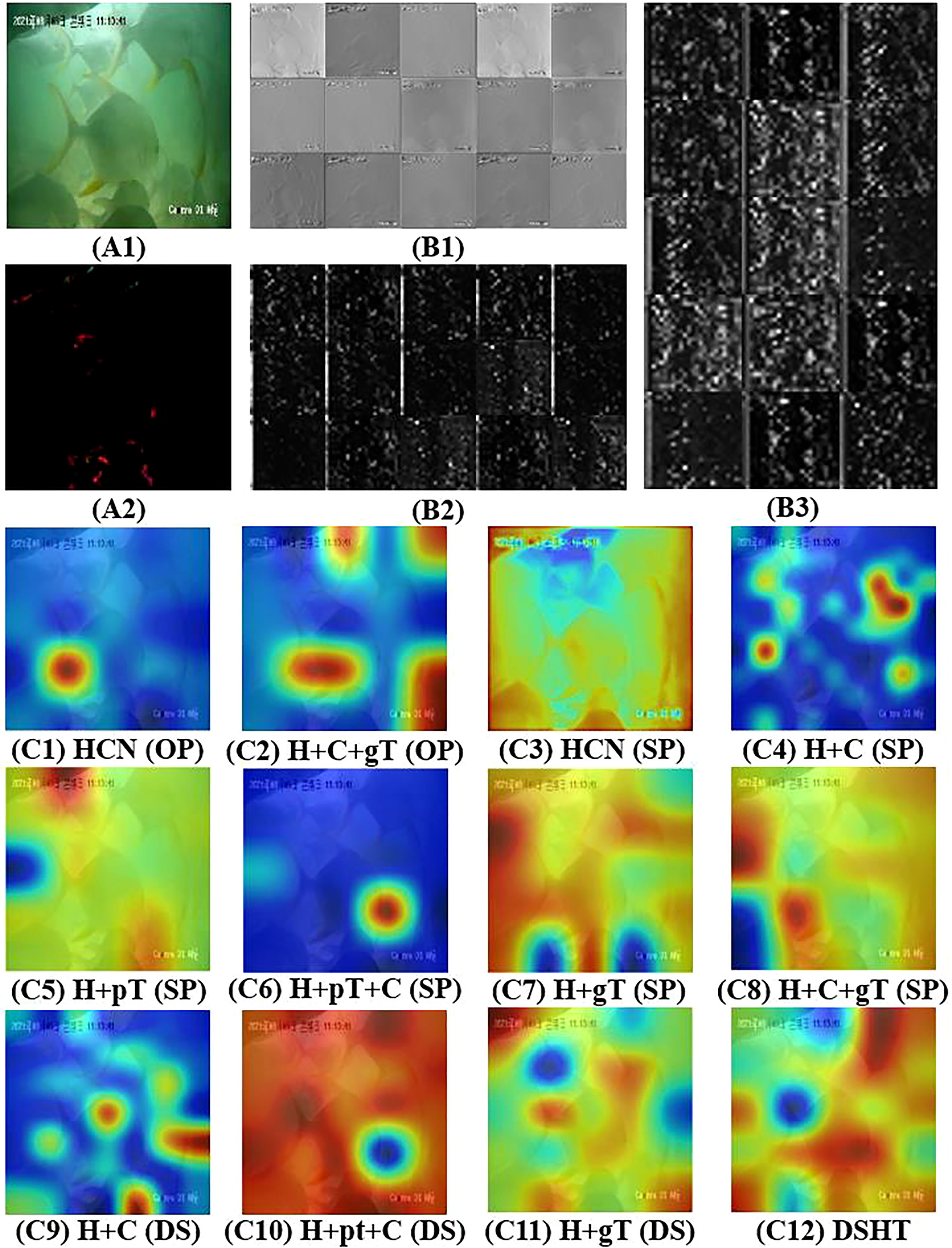
Figure 4 Visualization of Output Features. A1 is the spatial image which is fed into the spatial channel. A2 is the optical flow image which is fed into the temporal channle. B1 and B2 are DSHT’s hierarchical features in spatial and temporal channels, respectively. B3 is the output features of CFC in DSHT. From C1 to C12, respectively, they represent the Class Activation Map (CAM) of DSHT and other models mentioned in Ablation Experiments. H, C, gT, and pT are abbreviations for HCN, CFC, piecemeal Transformer, and global Transformer, respectively.

Comparison experiments

For the purpose of validating the reliability of proposed DSHT method, our model is compared with the following baselines in the same condition: VGG 16 (Simonyan and Zisserman, 2015), ResNet 18 (He et al., 2016), Mobile ViT (Mehta and Rastegari, 2022), Triplet Attention (Misra et al., 2021), Residual Attention (Zhu and Wu, 2021), DSRN (Måløya et al., 2019), DAN-EfficientNet-B2 (Yang et al., 2021) and DADSN (Zheng et al., 2022). The results are presented in Table 4. It shows that the DSHT model displays the best performance with the highest grading results in all metrics. The next one is the DADSN model with 83.43%, 84.52%, and 83.21% in the terms of accuracy, precision, and F1-scores, respectively. The worst are the VGG16 and DSRN models, which have only 20% accuracy, 4% precision, and 6.67% F1 score on the test set. The DAN-EfficientNet-B2 model also uses the structure with a CNN-based backbone and attention, but the grading results are not good, with each metrics in the range of 62% to 70%. Figure 5 shows the validation set correctness for each model during training. Figure 6 presents a schematic of the confusion matrix for the better performing models. Figure 7 is the grading results of DSHT model. Figure 8 display the visualization of the output features of each model.

TABLE 4

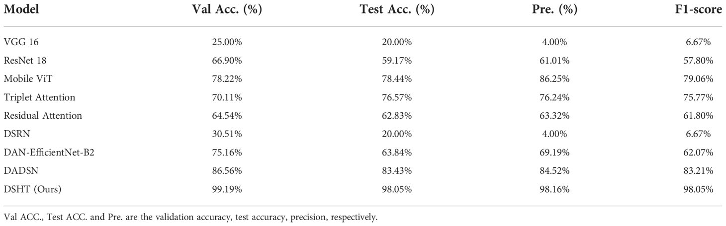
Table 4 The Grading Standards.

FIGURE 5

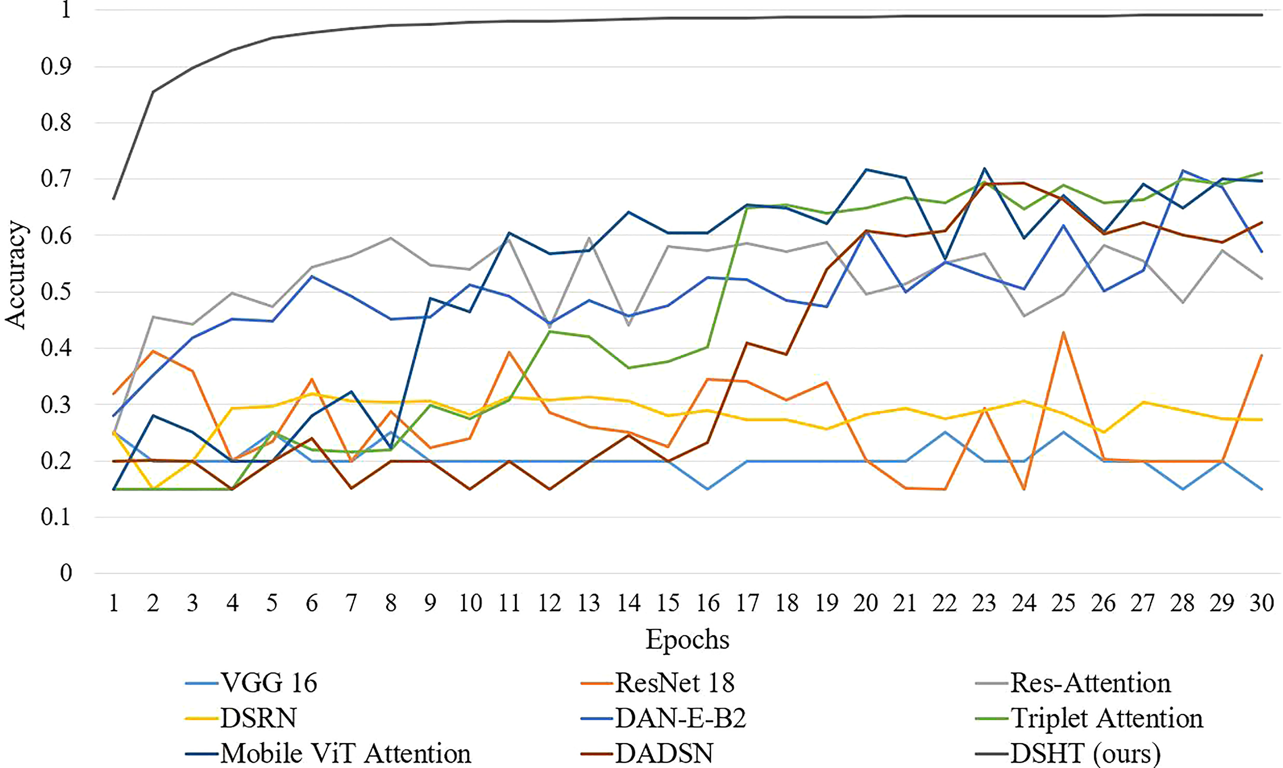
Figure 5 Validation Accuracy Curves of Comparison Models.

FIGURE 6

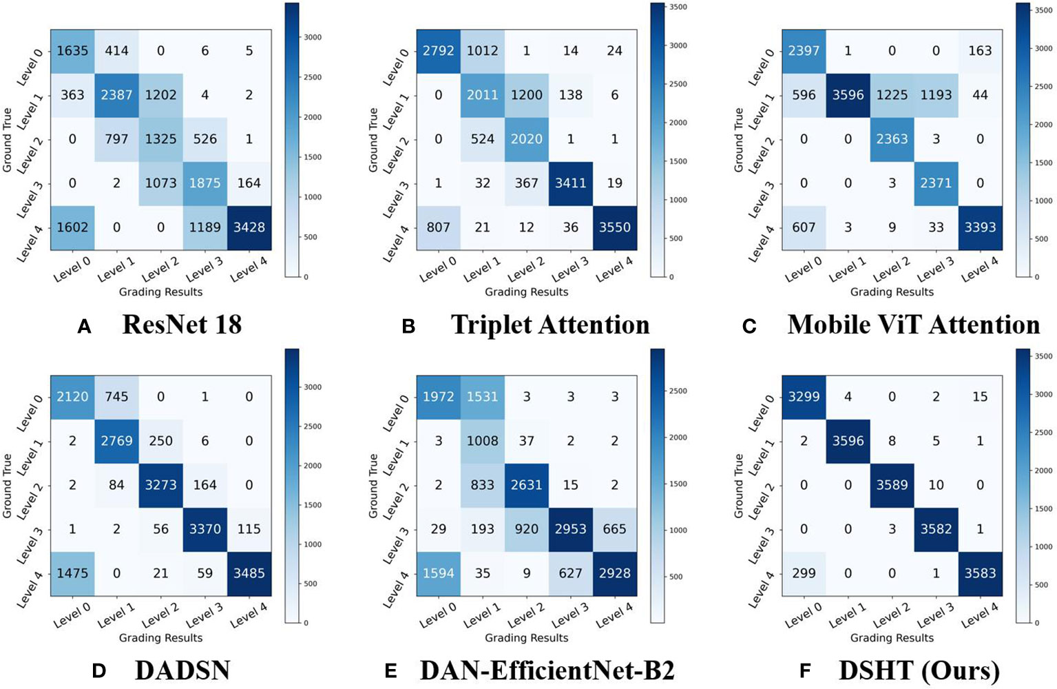
Figure 6 The Confusion Matrix. The experimental results of each model mentioned in Table 4 are shown, from (A–F), for ResNet 18, Triplet Attention, Mobile ViT Attention, DADSN, DAN-EfficientNet-B2, and DSHT (Ours). In the figure, each row represents the grading result of the model, and each column represents the true sample category. For example, in A, the first column of the first row indicates that: 1635 samples were grading correctly (true class L0 and graded result L0); the second column of the first row indicates that: 414 samples with true class L1 were graded as L0 by ResNet; the fourth column of the first row indicates that: 6 samples with true class L3 were graded as L0 by ResNet; the first column of the second row indicates that: 363 samples with true class L0 are graded as L1 by ResNet.

FIGURE 7

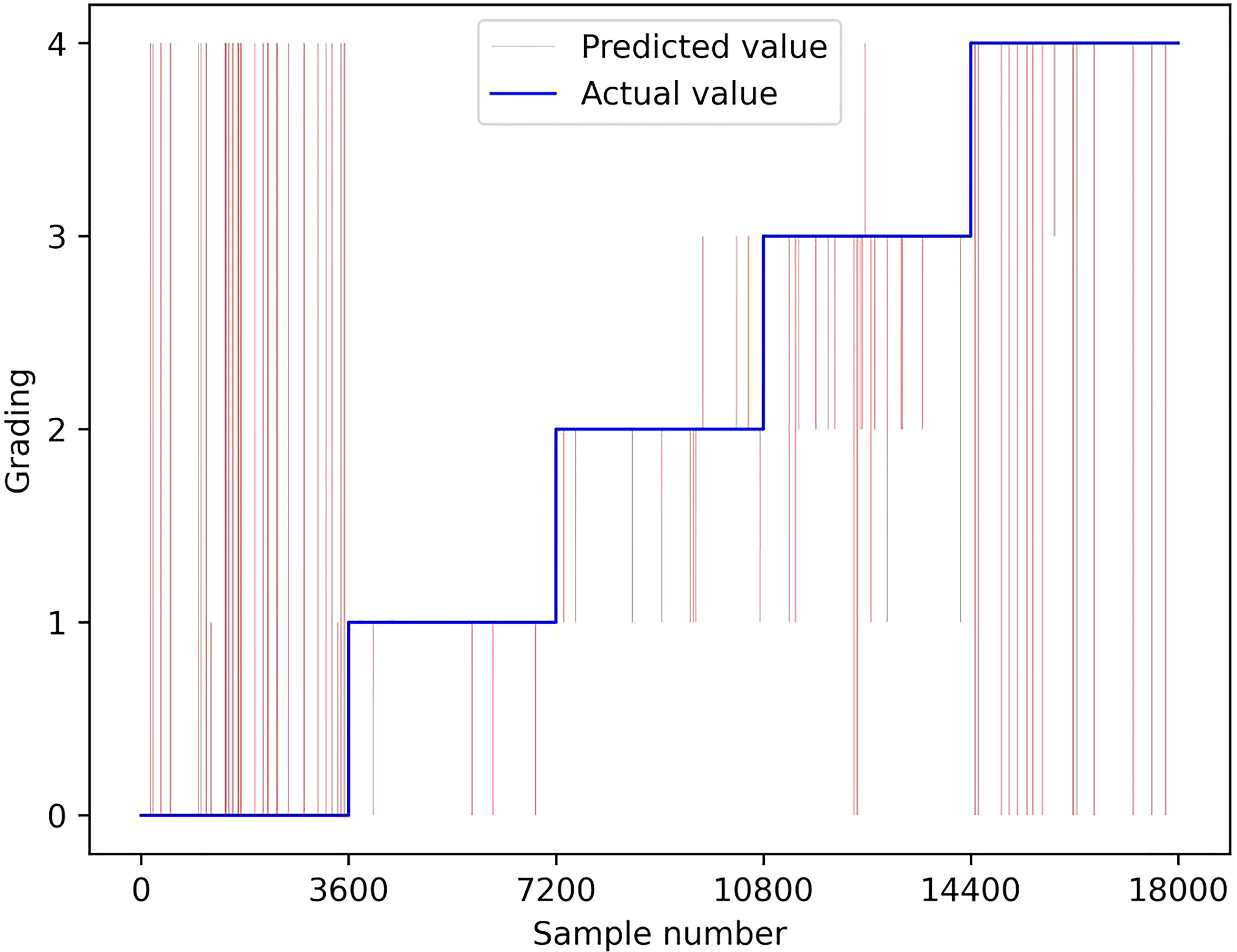
Figure 7 Grading Results of DSHT Model. The blue line is the ture value and the red line is the grading results predicted by DSHT.

FIGURE 8

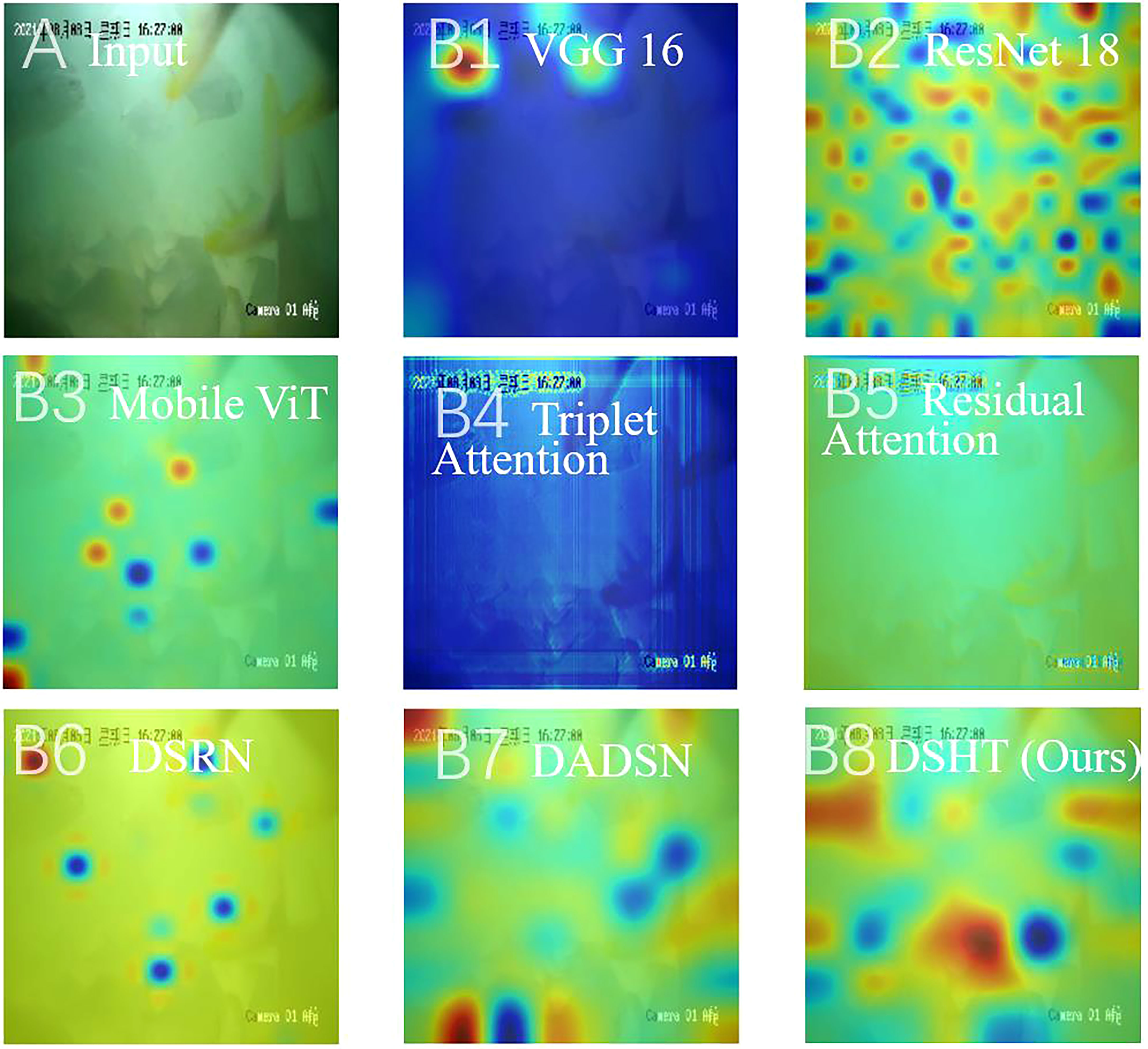
Figure 8 Class Activation Map (CAM) of Proposed Method and Other Methods. (A) is the input. From (B1–B8), the visualization results of the models in Table 4 are shown separately.

Discussion

In order to provide a more accurate feeding scheme for mariculture, fish starvation grading is one of the prerequisites for AI-feeding. Taking golden pomfret as the research target, this study attempts to realize automatic identification and monitoring of fish hunger status in the mariculture environment. Our aim is to solve the problem of precise feeding in deep-sea aquaculture and contribute to the development of unmanned and intelligent mariculture equipment. For this purpose, we proposed the Dual Stream Hierarchical Transformer (DSHT).

In the ablation experiment, we tested the modular performance of DSHT, including HCN, CFC, global Transformer and piecemeal Transformer in temporal channel, spatial channel and spatio-temporal channel. It was found that the grading results using a spatio-temporal channel (dual stream, DS) is better than temporal channel only (optical flow images only, OP) or spatial channel only (spatial images only, SP). To be specific, in the structure of HCN + CFC + global Transformer, the test accuracy, precision, and F1-score of DS are 98.05%, 98.16%, and 98.05%, respectively, which is better than the metrics of OP (80.09%, 82.77%, and 79.91%) and SP (90.85%, 93.49%, and 90.38%). The spatial channel provided spatial information, such as the number, distribution, and the mouth movements of fish in the image, while the optical flow images provided temporal information, such as the swimming speed, direction, and acceleration of fish school. As spatial and temporal channel provided unique information for starvation grading, they exhibited complementary effects when combined in the DSHT model. Furthermore, within certain short time interval (e.g., 0.5 seconds), if the object is not moving fast, a spatial image could provide rich detailed data during this time (e.g., whether the fish’s abdomen is bulging, whether the fish’s excrement appear in the image). In contrast, for consecutive images, because the time interval is extremely short and the images may not change to a great extent, they might provide duplicate information. This made some of them not relevant to the starvation grade (e.g., sunlight in the water), which led to misjudgment. We could not deny that continuous images can provide time-varying information that a single spatial image could not (e.g., swimming speed of the fish school), and this can also have an impact on the starvation grade. Therefore, we used optical flow images to reflect temporal information and experimentally demonstrated that the information provided by optical flow images can be used for starvation grading, with test accuracies of 67.97% and 80.09% for HCN (OP) and HCN + CFC + global Transformer (OP), respectively. In Figure 4 (C1), the temporal information is more concentrated on the tail of the fish, i.e., where the velocity changes faster, while in Figure 4 (C3), the spatial channel is more concentrated on the contour of the fish. Using a dual stream channel is a good way to enrich the input data in mariculture data. We also found that using the global transformer would be more effective than using the piecemeal transformer (the test accuracy of HCN + piecemeal Transformer (SP) is 76.21% and of HCN + global Transformer (SP) is 89.84%). This can be interpreted as the global transformer being calculated after the hierarchical features were integrated for attention, which overall filtering of useless features and marking which features should be attended to. In contrast, the piecemeal transformer is filtered each individual features separately and then integrated them at the end, so it resulted in poor attention to certain features. The local attention shown in Figure 4 (C6) visually demonstrates that the model was limited to a certain point, such as the fish mouth, compared to the global attention shown in Figure 4 (C8), where the model’s attention is not limited to a certain place. Compared with the experimental results of HCN + global Transformer (SP, 89.84%) and HCN + CFC + global Transformer (SP, 90.85%), HCN + global Transformer (DS, 95.72%) and HCN + CFC + global Transformer (DS, DSHT, 98.05%), it can be seen that the model using the CFC network outperforms the model without it. The CFC module is a feature fusion module that fuses hierarchical features from the HCN output in three different dimensions, indicating that our proposed DSHT with CFC fusion is more robust. Comparing Figure 4 (C3) and Figure 4 (C4), after adding CFC, the model starts to convert from the figurative feature of contour to the abstract feature.

Among the CNN-based models, VGG 16, ResNet 18, and HCN, where HCN has the best grading results, this indicated that our proposed model is more suitable for the mariculture environment of pomfret. Because HCN perceives the images with different sizes of kernels and outputs the low-dimensional features (e.g., the boundary of the fish) and high-dimensional features (e.g., the shape of the fish belly) of the images at the same time, HCN is more intuitive and concise than a single convolutional kernel that requires multiple perceptions to transition from low to high dimensions. By comparing the results of the attention-based models, Mobile ViT (78.44% accuracy), Triplet Attention (76.57% accuracy), Residual Attention (62.83% accuracy), and our proposed HCN + Transformer-based models (the accuracy ranged between 76.21% and 98.05%), we found that the performance of the HCN + Transformer performs better because the attention calculation of this model is performed at the feature level, which is the output of the HCN, while other models use attention calculation directly.

The DSRN, DAN-EfficientNet-B2 and DADSN are related researchers’ proposed models for fish behavior recognition. DSRN is used to classify the feeding or nonfeeding behavior of salmon in mariculture environments, and it uses 3D residual convolution and LSTM for feature extraction and feature filtering, respectively. The DAN-EfficientNet-B2 model divides the features into position attention and channel attention for recognizing fish feeding behavior. In this paper, we applied the DSRN and DAN-EfficientNet-B2 to the fish starvation grading task and found that their grading accuracy is not satisfactory (20.00% and 63.84% accuracy). We speculate that more fish information is required for the starvation grading task, and these models are difficult to meet the requirement using only 3D residual convolution or attention. This concept was also verified in the ablation experiment, where the accuracy of the dual stream model HCN + CFC (DS), which only used CNN-based structure, was only 82.46% in accuracy. But the DSHT, which used CNN-based and attention-based structures at the same time, can achieve 98.05%. Notably, the researchers (Zhou et al., 2019) used a 5-layer CNN to grade the intensity level of fish feeding, but when we migrated it to our task for testing, the experimental results were the same as VGG16. The DADSN model (83.43% accuracy) was used for the same starvation grading task as ours for the mariculture of pomfret. It adopted a modified Efficient network and ViT in each channel for feature extraction and attention computation, and uses LSTM to fuse the output features of each channel. Compared with our proposed DSHT model, DSHT does the attention operation in global features after CFC network fusion, while DADSN does it separately in spatial and temporal channels. Moreover, DSHT proposes a more concise multi-scale network HCN, which is another difference with DADSN.

Conclusions

In this paper, we study the starvation grading of golden pomfret school in a marine aquaculture environment. Establishing a dataset and proposing a DSHT model for this task. The DSHT uses a Hierarchical Convolutional Network to extract marine image features, which improves the effectiveness of the neural network in learning the starvation features of golden pomfret school. For the hierarchical features extracted by HCN, CFC is used for fusion, and a transformer is used to increase the weight of some regions that are favorable for starvation classification. To address the problem that fish behavior is temporal in nature, this paper designs a dual- stream structure by introducing optical flow images to increase temporal information. The effectiveness of each module proposed in this paper is demonstrated by ablation experiments. In the results of the comparison tests, DSHT achieved the best performance among all models involved. Experiments on a marine pomfret breeding vessel have shown that DSHT can be effectively applied to pomfret school starvation grading in marine images, with practical implications. In future research, we will explore how to use AI information for decision-making, control, and management of fish aquaculture.

Data availability statement

The original contributions presented in the study are included in the article/supplementary materials. Further inquiries can be directed to the corresponding author.

Ethics statement

Ethical review and approval were not required for the animal study because the data was collected under normal fish farming conditions.

Author contributions

KZ conceived the study and drafted the manuscript. RY provided critical revision of the article. RL designed the software. LY performed the analysis with the help from HQ. ZY participated in fish farming. All authors contributed to the article and approved the submitted version.

Funding

This work was supported by the Special Fund for Marine Economic Development (six marine industries) of Guangdong Province, China (GDNRC [2021]42), the Fund of Southern Marine Science and Engineering Guangdong Laboratory (Zhanjiang) (011Z21001), and the Fund of Zhanjiang Municipal Bureau of Science and Technology (2021E05034).

Acknowledgments

We wish to thank the Department of Natural Resources of Guangdong Province, the Zhanjiang Municipal Bureau of Science and Technology and the Southern Marine Science and Engineering Guangdong Laboratory (Zhanjiang) for funding this project. We thank Guangxi Jingong Marine Technology Co., Ltd. For providing the fingerlings and lures.

Conflict of interest

The authors declare that the research was conducted in the absence of any commercial or financial relationships that could be construed as a potential conflict of interest.

Publisher’s note

All claims expressed in this article are solely those of the authors and do not necessarily represent those of their affiliated organizations, or those of the publisher, the editors and the reviewers. Any product that may be evaluated in this article, or claim that may be made by its manufacturer, is not guaranteed or endorsed by the publisher.

References

Fu J., Liu J., Tian H., Li Y., Bao Y., Fang Z., et al. (2019). “Dual attention network for scene segmentation,” in The IEEE/CVF International Conference on Computer Vision 2019 (Piscataway, NJ: IEEE). 3141–3149. doi: 10.1109/CVPR.2019.00326

CrossRef Full Text | Google Scholar

Hendrycks D., Gimpel K. (2016). Gaussian Error linear units. ArXiv. Prep. ArXiv. 1606, 8415. doi: 10.48550/arXiv.1606.08415

CrossRef Full Text | Google Scholar

He K., Zhang X., Ren S., Sun J. (2016). “Deep residual learning for image recognition,” in The IEEE/CVF International Conference on Computer Vision 2016. (Piscataway, NJ: IEEE). 770–778. doi: 10.1109/CVPR.2016.90

CrossRef Full Text | Google Scholar

Hossain M. E., Khan M. A., Saha S. M., Dey M. M. (2022). Economic assessment of freshwater carp polyculture in Bangladesh: Profit sensitivity, economies of scale and liquidity. Aquaculture 548 (1), 737552. doi: 10.1016/j.aquaculture.2021.737552

CrossRef Full Text | Google Scholar

Jonas J., Wolff V., Fricke-neuderth K., Mothes O. (2017). “Visual fish tracking: combining a two-stage graph approach with CNN-features,” in Oceans Aberdeen Conference 2017, (Piscataway, NJ: IEEE). 1–6. doi: 10.1109/OCEANSE.2017.8084691

CrossRef Full Text | Google Scholar

Jothiswaran V., Velumani T., Jayaraman R. (2020). Application of artificial intelligence in fisheries and aquaculture. Biotica. Res. Today 2 (6), 499–502. Available at: https://www.biospub.com/index.php/biorestoday/article/view/257

Google Scholar

Krizhevsky A., Sutskever I., Hinton G. E. (2012). ImageNet classification with deep convolutional neural networks. Commun. ACM 60 (6), 84–90. doi: 10.1145/3065386

CrossRef Full Text | Google Scholar

Lecun Y., Bottou L., Bengio Y., Haffner P. (1998). Gradient-based learning applied to document recognition. Proc. IEEE 86 (11), 2278–2324. doi: 10.1109/5.726791

CrossRef Full Text | Google Scholar

Lin G., Lin X. (2022). Bait input altered microbial community structure and increased greenhouse gases production in coastal wetland sediment. Water Res. 218, 118520. doi: 10.1016/j.watres.2022.118520

PubMed Abstract | CrossRef Full Text | Google Scholar

Lucas B. D. (1985). Generalized image matching by the method of differences. PhD. Dissertation, Carnegie Mellon University. doi: 10.5555/912172

CrossRef Full Text | Google Scholar

Maaz M., Shaker A., Cholakkal H., Khan S., Zamir S. W., Anwer R. M., et al. (2022). EdgeNeXt: efficiently amalgamated CNN-transformer architecture for mobile vision applications. ArXiv. Prep. ArXiv. 2206, 10589. doi: 10.48550/arXiv.2206.10589

CrossRef Full Text | Google Scholar

Måløya H., Aamodta A., Misimi E. (2019). A spatio-temporal recurrent network for salmon feeding action recognition from underwater videos in aquaculture. Comput. Electron. Agric. 167, 1–9. doi: 10.1016/j.compag.2019.105087

CrossRef Full Text | Google Scholar

Mehta S., Rastegari M. (2022). Separable self-attention for mobile vision transformers. ArXiv. Prep. ArXiv. 2206, 2680. doi: 10.48550/arXiv.2206.02680

CrossRef Full Text | Google Scholar

Misra D., Nalamada T., Arasanipalai A. U., Hou Q. (2021). “Rotate to attend: Convolutional triplet attention module,” in The IEEE/CVF Winter Conference on Applications of Computer Vision 2021. (Piscataway, NJ: IEEE) 3139–3148. doi: 10.1109/WACV48630.2021.00318

CrossRef Full Text | Google Scholar

Raghu M., Unterthiner T., Kornblith S., Zhang C., Dosovitskiy A. (2021). Do vision transformers see like convolutional neural networks? ArXiv. Prep. ArXiv. 2108, 8810. doi: 10.48550/arXiv.2108.08810

CrossRef Full Text | Google Scholar

Ranjan A., Black M. J. (2017). “Optical flow estimation using a spatial pyramid network. in: Computer vision and pattern recognition,” in The IEEE/CVF International Conference on Computer Vision 2017. (Piscataway, NJ: IEEE). 4161–4170. doi: 10.1109/CVPR.2017.291

CrossRef Full Text | Google Scholar

Simonyan K., Zisserman A. (2015). “Very deep convolutional networks for large-scale image recognition,” in International Conference on Learning Representations 2015, (Banff, Canada: OpenReview). 1–14. doi: 10.48550/arXiv.1409.1556

CrossRef Full Text | Google Scholar

Szegedy C., Liu W., Yangqing J., Sermanet P., Reed S., Anguelov D., et al. (2015). “Going deeper with convolutions,” in The IEEE/CVF Winter Conference on Applications of Computer Vision 2015, (Piscataway, NJ: IEEE). 1–9. doi: 10.1109/cvpr.2015.7298594

CrossRef Full Text | Google Scholar

Yang L., Yu H., Cheng Y., Mei S., Duan Y., Li D., et al. (2021). A dual attention network based on efficientNet-B2 for short-term fish school feeding behavior analysis in aquaculture. Comput. Electron. Agric. 187, 106316. doi: 10.1016/j.compag.2021.106316

CrossRef Full Text | Google Scholar

Ye Z., Zhao J., Han Z., Zhu S., Li J., Lu H., et al. (2016). Behavioral characteristics and statistics-based imaging techniques in the assessment and optimization of tilapia feeding in a recirculating aquaculture system. Trans. ASABE. 59, 345–355. doi: 10.13031/trans.59.11406

CrossRef Full Text | Google Scholar

Zhao J., Bao W., Zhang F., Zhu S., Liu Y., Lu H. D., et al. (2018). Modified motion influence map and recurrent neural network-based monitoring of the local unusual behaviors for fish school in intensive aquaculture. Aquaculture 493, 165–175. doi: 10.201016/j.aquaculture.2018.04.064

CrossRef Full Text | Google Scholar

Zheng K., Yang R., Li R., Yang L., Qin H., Sun M. (2022). “A deep transformer model-based analysis of fish school starvation degree in marine farming vessels,” in 2022 4th International Conference on Control and Robotics (ICCR), Guangzhou, China. (Piscataway, NJ: IEEE).

Google Scholar

Zhou C., Xu D., Chen L., Zhang S., Sun C., Yang X., et al. (2019). Evaluation of fish feeding intensity in aquaculture using a convolutional neural network and machine vision. Aquaculture 507, 457–465. doi: 10.1016/j.aquaculture.2019.04.056

CrossRef Full Text | Google Scholar

Zhou C., Zhang B., Lin K., Xu D., Chen C., Yang X., et al. (2017). Near-infrared imaging to quantify the feeding behavior of fish in aquaculture. Comput. Electron. Agric. 135, 233–246. doi: 10.1016/j.compag.2017.02.013

CrossRef Full Text | Google Scholar

Zhu K., Wu J. (2021). “Residual attention: A simple but effective method for multi-label recognition,” in The IEEE/CVF International Conference on Computer Vision 2021, (Piscataway, NJ: IEEE). 184–193. doi: 10.1109/ICCV48922.2021.00025

CrossRef Full Text | Google Scholar