Decadal intensified and slantwise Subpolar Front in the Japan/East Sea

The Subpolar Front in the Japan/East Sea (JES) could far-reaching influence the atmospheric processes over the downstream regions. However its variability on decadal timescale remains less understood. In this study, the decadal trends in the intensity and position of the SPF in the JES during the time period 1985−2020 are analyzed by using four categories of satellite observed high-resolution sea surface temperature products. The results show that there is a significant intensification trend of the SPF at a rate of 0.37°C/100km/decade. The SPF is further divided into three regions based on the meridional sea surface temperature gradient (MSSTG): the eastern (135−138°E), central (130−135°E) and western (128−130°E) regions, respectively. These three regions showed different meridional movements with the eastern SPF moving poleward by 0.08°/decade, the central SPF moving equatorward by −0.11°/decade and the western SPF showing no significant displacements. The reverse meridional movements between the central and eastern SPF increased its skewness. The frontogenesis rate equation is employed to identify the mechanisms of these decadal trends. Results show that the geostrophic advection term, especially its zonal component, had a crucial role in the decadal trends of the intensity and position of the central and eastern SPF. The decadal trend of the central SPF was mainly attributed to the zonal geostrophic advection of the MSSTG associated with the enhancement of the Subpolar Front Current (SFC) in the upstream region, whereas the decadal trend in the eastern SPF was mainly driven by the zonal geostrophic shear advection controlled by the shear of the SFC in the downstream region. Before 2002, the eastern SPF moved poleward at a rate of 0.27°/decade, whereas there was no obvious trend after 2002. Further decomposition showed that this shift was caused by meridional Ekman advection of the MSSTG.

1 Introduction

Oceanic fronts are common at the surface of the ocean and are accompanied by intensified spatial differences in hydrographic properties (e.g., temperature, salinity and biogeochemical characteristics). The distinct features of fronts include a large gradient in one horizontal direction accompanied by a weak gradient in the perpendicular horizontal direction (McWilliams, 2021). The atmospheric conditions in mid-latitude regions are influenced by fronts, such as the Subtropical Front and Subpolar Front (SPF), through vertical mixing and pressure adjustments, especially in the western boundary currents and their regions of extension, with a high sea surface temperature (SST) gradient and the loss of heat to the atmosphere (Minobe et al., 2008; Takatama et al., 2015). The meridional shift in SST fronts could change distribution of SST (Pak et al., 2017) and influence both the intensity and position of storm track activity (Ogawa et al., 2012).

Recent studies reported a consistent poleward shift in the fronts of the major ocean gyres of the open oceans (Yang et al., 2016; Yang et al., 2020a; Yang et al., 2020b), with an average frontal shift rate of 0.07°/decade. However, the shift trends are dependent on the region—for example, the fronts in the North Atlantic Ocean were reported to have the smallest shift rate and showed a trend of shifting toward the equator from the 1990s to the 2000s (Joyce et al., 2000; Frankignoul et al., 2001). The shift trends of the Oyashio Extension front in the North Pacific are dependent on longitude, with the eastern branch in the open sea showing a significant poleward shift trend of 0.18°/decade, whereas the western branch near the coast shows no obvious poleward shift (Wu et al., 2018; Wu et al., 2019).

Many factors affect the strength and location of fronts, including wind stress, ocean currents, and the heat flux. The movement of SST fronts in the Kuroshio–Oyashio Extension region has been attributed to basin-scale and local wind forcing via barotropic and baroclinic Rossby wave propagations (Kwon et al., 2010; Pak et al., 2017) and movement of the zero wind stress curl line (or the zero Sverdrup streamline) (Wu et al., 2018; Wu et al., 2019). Thermodynamic processes induced by the oceanic advection of heat also contribute to the variability of the position and intensity of the SST fronts (Wu et al., 2018; Wu et al., 2019). After the 1990s, the fronts in the Gulf Stream region showed a reverse direction of shift from that before the 1990s, mainly caused by the North Atlantic Oscillation, which regulates the position of the North Atlantic Subtropical Gyre, shifting from a positive to a negative phase. The fronts moved poleward during the positive phases of the North Atlantic Oscillation and equatorward during the negative phases (Joyce et al., 2000; Frankignoul et al., 2001). The Gulf Stream shifted equatorward in the Slope Water region as a result of transport by the larger deep western boundary current (Peña-Molino and Joyce, 2008).

The Japan/East Sea (JES) is a semi-enclosed marginal sea in the Northwestern Pacific that contains many similar features and elements to the open ocean, such as gyre circulations, eddies, an SPF and water mass—it is often referred to as a “miniature ocean” (Chang et al., 2016).The JES is an ideal natural laboratory in which to study oceanic processes and their response to global climate change. The SPF in the JES is the boundary between the warm water supplied by the Tsushima Warm Current (TWC) across the Korea/Tsushima Strait (KTS) in the south and relatively cold water over the deep Japan Basin in the north. The SPF has an important impact on the water mass, mesoscale eddies and winter convection in the JES (Yoshikawa et al., 1999; Ou and Gordon, 2002).

Early studies using infrared images showed the existence of horizontal structures and the seasonal variability of the SPF in the JES (Legeckis, 1978; Huh, 1982). The SST gradient of the SPF is strongest in winter and weakens to 3°C/100km or less in summer, accompanying the distribution of the SPF from the southwest to the northeast in winter and from the northwest to southeast in summer (Park et al., 2004; Park et al., 2007). In terms of the seasonal frontogenesis processes, the mixed-layer model and oceanic reanalysis data showed that horizonal advection is dominant throughout the year, especially the geostrophic component (Zhao et al., 2014). With respect to the seasonal frontolysis processes, the surface heat flux has a dominant role in all months, especially in spring and summer (Ohishi et al., 2019), and also causes weakening or even the disappearance of the SPF (Park et al., 2007). In autumn and winter, the mixed-layer gradient damps the frontolysis induced by the surface heat flux (Ohishi et al., 2019). However, a detailed description of the decadal variations and mechanisms of the SPF are yet to be addressed, partly due to the limited duration of observations—for example, numerical simulations have shown that the interannual variability of the SPF from 1993 to 2001 was strongly affected by wind stress and transport of the TWC (Choi et al., 2009).

It is still an open question as to whether the intensification and poleward movement of SST fronts are present in marginal seas such as the JES. Satellite-based SST observations have been collected for almost four decades and provide a unique opportunity to explore the decadal variations of the SPF in the JES. In this study, four satellite-observed SST products with different sensors are employed to study the decadal variations in the intensity and position of the SPF. Section 2 introduces the data and methods, Section 3 gives the results for the satellite-observed SPF, Section 4 discusses the possible mechanisms and Section 5 summarizes our conclusions.

2 Data and methods

2.1 Data

Four SST datasets are used to characterize the decadal variations in the JES SPF during the time period 1985–2020: the Coral Reef Watch satellite SST product (CoralTemp Version 3.1), the Optimum Interpolation SST (OISST Version 2.1), the SST record produced by the European Space Agency and the Copernicus Climate Change Service (ESASST), and Operational Sea Surface Temperature and Sea Ice Analysis (OSTIA). CoralTemp is the product of the National Oceanic and Atmospheric Administration (NOAA) Coral Reef Watch program, which blends SSTs from geostationary and polar-orbiting infrared satellites (Skirving et al., 2020). CoralTemp Version 3.1 is a daily global 5 km night-time SST product from January 1985 to the present day. The NOAA OISST Version 2.1 (Huang et al., 2021) is a daily global 0.25° SST product from September 1981 to the present day. It blends Advanced Very High-Resolution Radiometer (AVHRR) infrared satellite SST data and in situ observational data from ships and buoys. The OSTIA system was developed at the UK Met Office as the UK’s contribution to the International Group for High Resolution SST (Good et al., 2020). OSTIA is a daily global 5 km SST product from October 1981 to present day. It blends satellite infrared and microwave SST data and in situ observational data. ESASST is a daily global 5 km SST product from September 1981 to the present day. It blends AVHRR, Along-Track Scanning Radiometers and Sea and Land Surface Temperature Radiometer data to give a stable product (Merchant et al., 2019). We chose the same time period for all four products (1985–2020).

The wind and heat flux data are from the Fifth Generation European Centre for Medium Range Weather Forecasts Reanalysis (ERA5) dataset for the global climate and weather (Hersbach et al., 2019). The ERA5 data are available from 1950 to the present day and the same time period as for the SST data (1985–2020) are employed. The geostrophic surface velocity and absolute dynamics topography with a horizontal resolution of 0.25° during the time period 1993–2020 are from Copernicus climate data storge. An observational dataset (the EN4 data) is used to calculate the mixed-layer depth (MLD). The EN4 data (version EN.4.2.2-analyese-g10) produced by the UK Met Office Hadley Center (Gouretski and Reseghetti, 2010) is a global gridded monthly objective analysis of in situ observations.

2.2 Definition of the SPF

In this study, monthly-mean SST data are used to estimate the intensity and position of the SPF (Kida et al., 2015). The frontal intensity was obtained from the absolute value of the maximum meridional SST gradient (MSSTG) at each longitude between 38 and 41°N. The position of the SPF is defined as the latitude of the maximum MSSTG. Given that the SPF in the JES turns poleward at the eastern end, the front is defined as eastward until 138°E (Park et al., 2004; Park et al., 2007). The monthly intensity and position were processed into an annual mean to remove the seasonal variability. The statistical significance of the trend was tested using the Mann–Kendall test (Xu et al., 2021). SST data shallower than 200 m were removed to exclude the effects of coastal variations (e.g., runoff and upwelling).

2.3 Frontogenesis rate equation

The temperature tendency equation in the surface mixing layer can be written as:

$\begin{array}{ll}\frac{\partial T}{\partial t}=\frac{Q_{net}}{\rho C_{p}h}-\overrightarrow{V}·\nabla T-\frac{w_e\Delta T}{h}& (1)\end{array}$

Where T is the SST. The left-hand side (LHS) of the equation is the SST tendency term. Here, Q_net is the net heat flux (NHF, with positive values indicating the ocean gaining heat from the atmosphere), ρ (1025 kg/m³) is the density of seawater, C_p (3986 J/kg/°C) is the specific heat of seawater and h is the MLD estimated from the EN4 data according to a temperature-based threshold Δθ, which is set to 0.2°C (Lim et al., 2012). The first term on the right-hand side (RHS) is referred to as the NHF/MLD term. The second term on the RHS of equation (1) ($(\overrightarrow{V}·\nabla T)$) represents horizontal advection, where $\overrightarrow{V}$ is the horizontal current vector. The third term (w_e·ΔT/h) is the entrainment term, where ΔT is the temperature difference between the mixed layer and the layer just below, which is also set to 0.2°C. The entrainment speed w_e is simply represented by the Ekman pumping velocity:

$\begin{array}{ll}{w}_e=cur{l}_z\left(\frac{\overrightarrow{\tau }}{\rho f}\right)& (2)\end{array}$

where $\overrightarrow{\tau }$ is the wind stress vector calculated from the bulk formula ($\overrightarrow{\tau }={\rho }_{air}{C}_D\left|{\overrightarrow{U}}_{10}\right|{\overrightarrow{U}}_{10}$) and ${\overrightarrow{U}}_{10}$ is the 10 m wind vector from the ERA5 dataset. The air density (ρ_air) is 1.2 kg/m³, C_D is the nonlinear drag coefficient calculated following Large and Pond (1981) and f the Coriolis parameter.

The frontogenesis rate equation can be derived from the meridional derivative of the temperature tendency equation in equation (1):

$\begin{array}{ll}\frac{\partial }{\partial t}\left(-\frac{\partial T}{\partial y}\right)=-\frac{\partial }{\partial y}\left(\frac{Q_{net}}{\rho C_{p}h}\right)+\frac{\partial }{\partial y}\left(\overrightarrow{V}·\nabla T\right)+\frac{\partial }{\partial y}\left(\frac{w_e\Delta T}{h}\right)& (3)\end{array}$

where y is the meridional coordinate. The LHS of equation (3) is the frontogenesis rate term. Note that equation (3) is multiplied by -1 to specify that positive (negative) values refer to frontogenesis (frontolysis). Considering the contributions of the Ekman and geostrophic advections in the JES (Zhao et al., 2014), the horizontal advection gradient term $\partial \left(\overrightarrow{V}·\nabla T\right)/\partial y$ can further be decomposed into:

$\begin{array}{ll}\frac{\partial }{\partial y}\left(\overrightarrow{V }·\nabla T\right)=\frac{\partial }{\partial y}\left({\overrightarrow{V}}_{ek}·\nabla T\right)+\frac{\partial }{\partial y}\left({\overrightarrow{V}}_{geo}·\nabla T\right)& (4)\end{array}$

Where the Ekman currents are calculated using:

$\begin{array}{ll}{\overrightarrow{V}}_{ek}=\frac{{\tau }_y}{\rho fh}\overrightarrow{i}-\frac{{\tau }_x}{\rho fh}\overrightarrow{j}& (5)\end{array}$

where τ_x and τ_y are the zonal and meridional surface wind stress, respectively, and $\overrightarrow{i}$ and $\overrightarrow{j}$ are the zonal and meridional unit vectors, respectively. The horizontal advection gradient term can be decomposed into the processes that act to generate or destroy the SPF:

$\begin{array}{ll}\frac{\partial }{\partial y}\left(\overrightarrow{V}\cdot \nabla T\right)=\underset{Total U advection}{\underbrace{\frac{\partial u}{\partial y}\frac{\partial T}{\partial x}+u\frac{\partial }{\partial x}\left(\frac{\partial T}{\partial y}\right)}}+\underset{Total V advection}{\underbrace{\frac{\partial v}{\partial y}\frac{\partial T}{\partial y}+v\frac{\partial }{\partial y}\left(\frac{\partial T}{\partial y}\right)}}& (6)\end{array}$

Each term on the RHS of equation (6) is the contribution resulting from temperature advection by zonal shear and meridional convergence (the first and third terms on the RHS, respectively) and the zonal and meridional advection of the MSSTG (the second and fourth terms on the RHS, respectively).

All the data used in the frontogenesis rate equation were processed into monthly average values and interpolated to a (1/4°×1/4°) grid. The results from the frontogenesis rate equation were averaged to the annual mean to remove the seasonal variability. Both terms were spatially smoothed with a window size of (6°×4°) to suppress the mesoscale eddies (Sasaki and Schneider, 2011; Pak et al., 2017). The flowchart of the datasets and data processing in the frontogenesis rate equation diagnosis is provided in the Supplementary Material (Figure S1).

2.4 Estimation of steric and non-steric height

To obtain better insight into the geostrophic current variation, different components contributing to the sea surface height variation were estimated. The steric height is the component of sea level variation representing changes in the density of the water column which imply an expansion or contraction of the column. Following Gill and Niller (1973), the steric height can be estimated as:

$\begin{array}{ll}{{\eta }^{\prime }}_{Steric}=-\frac{1}{{\rho }_0}{\displaystyle {\int }_{-H}^0{\rho }^{\prime }dz}& (7)\end{array}$

Where ρ′ represents the density anomaly of seawater from its climatology, calculated by EN4 data. H was chosen to be an assumed level of no motion, 1000m for example. The steric height was integrated from 0-1000m (or the water bottom for shallower regions) with 1m intervals by applying the spline interpolation method of Akima (1970). ρ₀ is a representative seawater density constant. Thus, the non-steric component ${\eta }_{Nonsteric}^{\text{'}}$ was obtained by removing the steric component ${\eta }_{Steric}^{\text{'}}$ from total sea level anomaly (SLA) variation ${\eta }^{\prime }$ as in equation (8):

$\begin{array}{ll}{\eta }_{Nonsteric}^{\text{'}}={\eta }^{\prime }-{\eta }_{Steric}^{\text{'}}& (8)\end{array}$

${\eta }^{\prime }$ is provided by satellite altimeter product from Copernicus climate data storge.

3 Decadal variations in the intensity and position of the SPF

Figure 1 shows the climatological absolute value, position and intensity of the SPF calculated from the MSSTG with the seven-year running average based on CoralTemp (the results for the other three products are shown in Figures S2–S4). The characteristics of the SPF calculated by the MSSTG are consistent with the SPF defined by whole horizontal SST gradient (Ohishi et al., 2019). There are three regions along the SPF with large SST gradients (>4°C/100km). The first is located east of 135°E, with a maximum >4.5°C/100km. The second is in the central JES (133–135°E). The third is located west of 130°E. We therefore divided the SPF into three regions: an eastern (135–138°E), central (130–135°E) and western (128–130°E) region. There are two branches in the western JES with a gradient >1.5°C/100km, one is a northwestern branch originating from Peter the Great Bay, whereas the other is the southwestern branch originating from the East Korean Bay. The northwestern branch is seasonal (Park et al., 2004; Park et al., 2007) and was therefore not considered in this study.

FIGURE 1

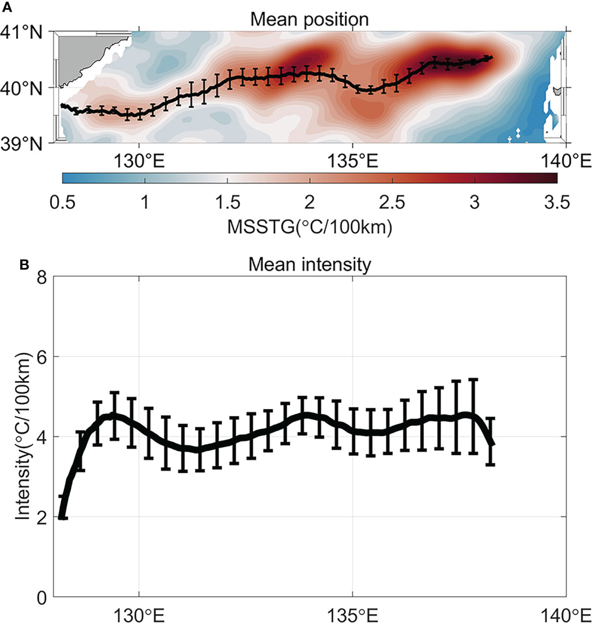
Figure 1 (A) The climatological position of the SPF (black lines) in the JES, and the climatological absolute value of the MSSTG (color shaded, unit: °C/100km). (B) The climatological intensity (unit: °C/100km) of the SPF. Error bars are the standard deviations calculated by the MSSTG with seven-year running average.

The differences in the SST and MSSTG between the two time periods of 1985–1994 and 2011–2020 were calculated, which could be regarded as the decadal trends from 1985 to 2020 (Figure 2). The SST warmed over the whole of the JES, except in the central region, similar to the results of Lee and Park (2019); Chen et al. (2022) and Jeong et al. (2022), suggesting equatorward movement of the SPF in this region. The equatorial flank of the eastern SPF warmed faster than the polar flank, implying a poleward shift. However, there was no remarkable difference in the warming trend shows between the two flanks of the western SPF. These meridional movements were also seen in the MSSTG field. The enhanced MSSTG over the polar flank of the eastern SPF shows that the frontal axis moved poleward, whereas the increasing (decreasing) trends of the MSSTG were seen over the equatorial (polar) flank of the central SPF, implying equatorward movement. The characteristics of the longitude-dependent meridional shift characteristics were different from those in the open ocean, where there is a consistent poleward movement (Wu et al., 2018; Wu et al., 2019; Yang et al., 2020a; Yang et al., 2020b). The slantwise change of the SPF in the JES was only present locally.

FIGURE 2

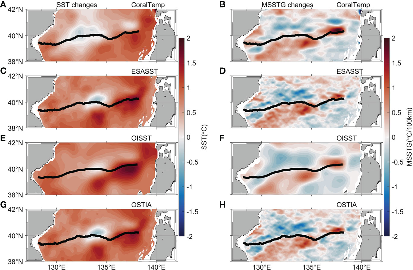
Figure 2 Decadal changes of (A) SST (unit: °C) and (B) the absolute value of the MSSTG (unit: °C/100km) between 1985–1994 and 2011–2020 (the latter minus the former). Shown are (left) SST (right) MSSTG based on (A, B) CoralTemp, (C, D) ESASST, (E, F) OISST and (G, H) OSTIA, respectively. Black lines indicate climatological position of the SPF during the time period of 1985–2020.

Figure 3 shows the linear trends of the SPF at each longitude to quantify the long-term variations in its intensity and position. Although the amplitudes of the intensity trend vary among the different SST products, they all show a significant intensification signal and consistent zonal distribution (Figure 3A; black solid line indicates the multidata average trend). The maximum mean increased trend was >0.8°C/100km/decade near 137.5°E. There was a clear poleward movement (with an average rate of 0.08°/decade) of the eastern SPF and an equatorward shift (at an average rate of −0.11°/decade) of the central SPF, but no significant shift trend in the western SPF (Figure 3B). The maximum poleward (equatorward) shift in the central (eastern) SPF exceeded 0.1°/decade (−0.15°/decade), as shown in Figure 3B. The magnitudes of the meridional movements of the SPF in the JES were comparable with those in the open ocean (Wu et al., 2018; Wu et al., 2019). There were two fluctuations in the central SPF where the most equatorward displacements were at 132 and 134°E (Figure 3B).

FIGURE 3

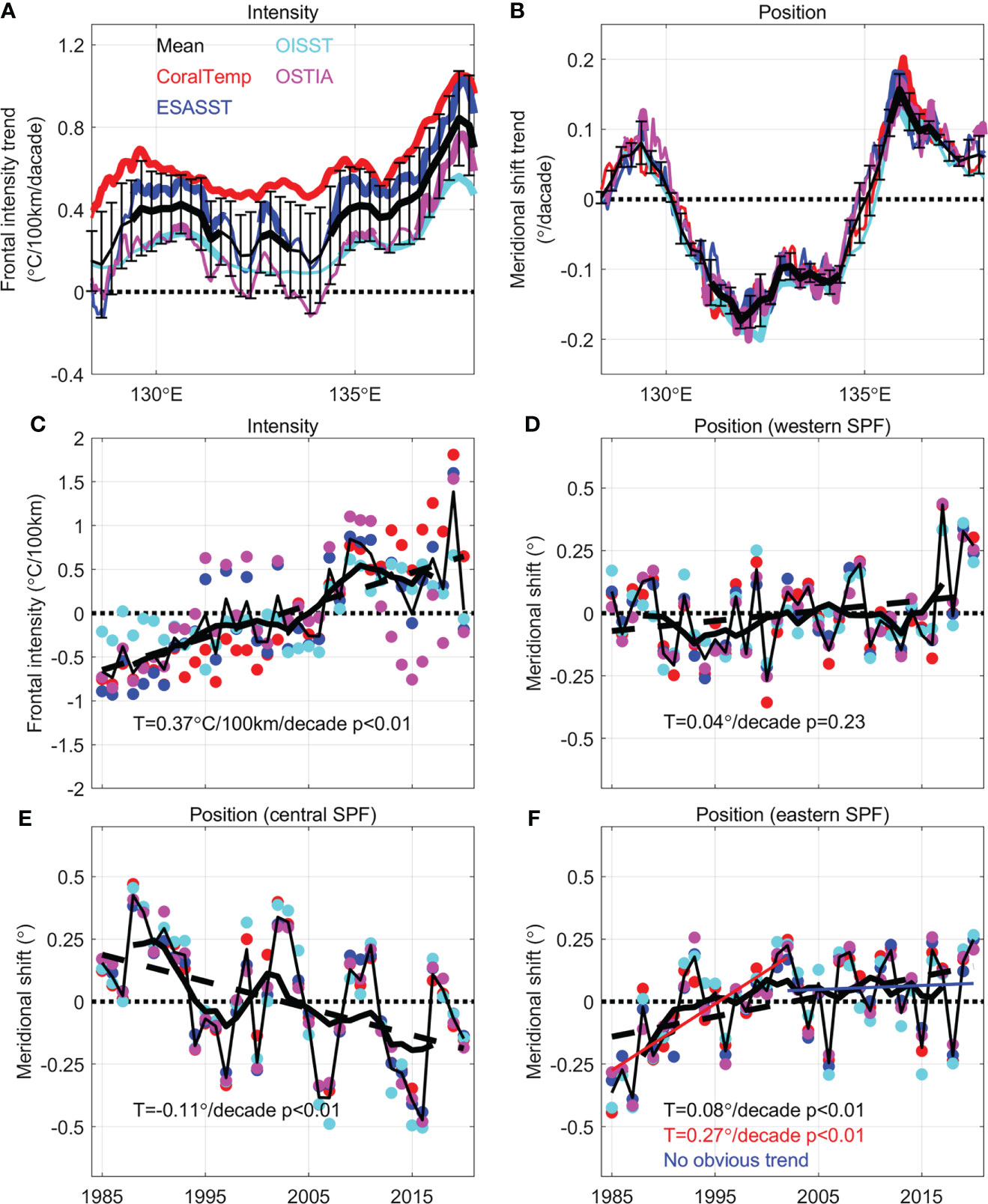
Figure 3 Zonal distribution of linear trends for (A) intensity (unit: °C/100km/decade) and (B) position (°/decade) of the SPF. Black, red, blue, cyan, and magenta solid lines are the results of mean, CoralTemp, ESASST, OISST and OSTIA, respectively, and thicker lines indicate statistical significance passing 95% confidence level. Error bars are the standard deviation among four SST datasets. (C) Time series of annual mean intensity (°C/100km) of the SPF. Red, blue, cyan and magenta solid dots represent results from four SST datasets as in (A, B). Black solid lines represent multidata mean (thin line) and seven-year running averages (thick line). Black dashed line indicates linear trend. (D-F) Same as (C) but for annual mean positions for (D) western SPF, (E) central SPF and (F) eastern SPF. The corresponding linear trends (T) are given by the text, and the associated p values (p)re also given based on the Mann-Kendall test. The red and blue lines in (F) indicate the eastern SPF shift trend before and after 2002, respectively.

Figure 3C shows the evolution of the intensity of the zonally averaged SPF. Although there were uncertainties among the different datasets, the SPF has consistently strengthened over the last 36 years. The rate of intensification was 0.37°C/100km/decade based on the average dataset. Figures 3D-F shows the time series of the position of the zonally averaged western, central and eastern SPF, respectively. Similar to the results shown in Figure 2 and Figure 3B, the poleward shift of the western SPF was not statistically significant (Figure 3D). The consistent equatorward movement of the central SPF was robust (Figure 3E). The poleward shift of the eastern SPF showed a decadal shift before and after 2002 (Figure 3F). During the first period (1985–2002), the eastern SPF shifted poleward at a rate of 0.27°/decade, which is faster than the mean rate (0.08°/decade) in the whole 36-years period. However, after 2002, there was more interannual variability than the decadal trend. The fact that the poleward shift of the eastern SPF mainly occurred before 2002 agrees with the movement of the Kuroshio Extension Front in the North Pacific (Wu et al., 2021). The time series of the position of the central and eastern SPF also showed strong variability on interannual to decadal time scales. There was a meridional movement of 0.5–1° in latitude on timescales of 5–10 years. For example, the central SPF was located relatively poleward in the early 1990s, 2000s and 2010s, but more equatorward in the years around 1996, 2006 and 2016 (Figure 3E). To emphasize the decadal trend, the time series of the intensity and position of the SPF with the seven-year running average are shown as thick, black solid lines. The intensification and slant of the SPF remained robust.

4 Possible mechanisms

We have shown that both the central and eastern SPF intensified over the study period but had the opposite meridional movements. There are many mechanisms that could contribute to these differences. For example, the entrance of the TWC into the JES will affect the SPF, especially in the south (Park et al., 2007). The monsoon also forces the JES with the strong westerly winds from Vladivostok Gap in winter, inducing strong cold currents and pushing cold water equatorward. Ohishi et al. (2019) pointed out that the NHF tends to relax the SPF throughout the year, however, the MLD can dampen (enhance) the frontolysis induced by the NHF in winter (summer). The possible mechanisms of the oceanic and atmospheric factors are explored by the frontogenesis rate equation (equation 3). We focused on the central and eastern SPF because there was no clear shift in the western SPF. Geostrophic currents are available from 1993, we examined the decadal changes between the time periods 1993–2002 and 2011–2020.

4.1 Frontogenesis rate equation diagnosis

Figure 4 shows the decadal changes in the MSSTG in the periods 1993–2002 and 2011–2020 calculated using each term of equation (3). The decadal changes in the MSSTG calculated from the observations and the frontogenesis rate term show similar patterns (Figures 4A, B). The decadal changes in the MSSTG caused by the geostrophic advection gradient term (Figure 4D) show positive (negative) values over the polar (equatorial) flanks of the eastern SPF. The geostrophic advection term shows negative (positive) values over the polar (equatorial) flanks in the central SPF. This pattern is consistent with the meridional shift and intensification in the central and eastern SPF (Figures 2B, D, F, H). This spatial pattern means that the geostrophic advection gradient term acts to intensify the SPF and move the central SPF toward the equator and the eastern SPF toward the polar. By contrast, the Ekman advection gradient term shows consistent intensification in the central SPF, but the opposite changes in the eastern SPF (Figure 4C). The decadal changes in the MSSTG induced by the NHF/MLD gradient term (Figure 4E) show positive (negative) values over the polar (equatorial) flanks in the central and eastern SPF. This indicates that the NHF/MLD gradient term dampens (enhances) the equatorward (poleward) shift of the central (eastern) SPF. The contribution from the entrainment gradient term is small and can be ignored (Figure 4F).

FIGURE 4

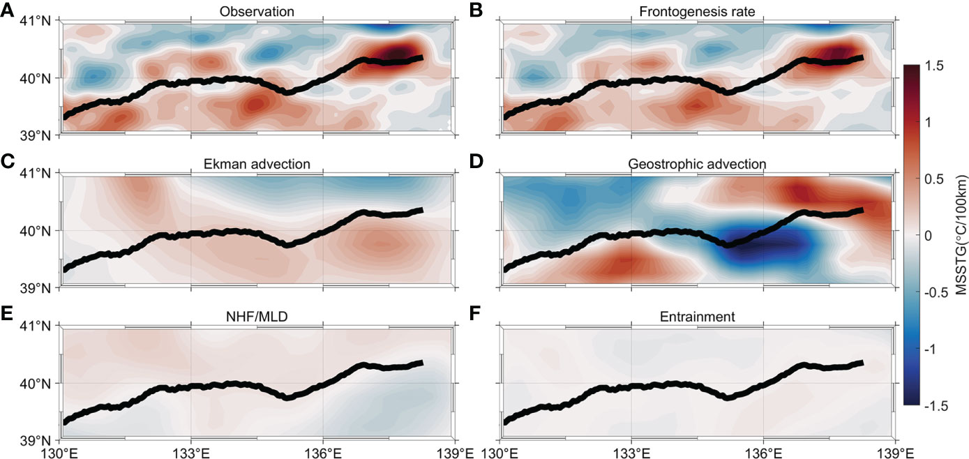
Figure 4 (A) The decadal change in the MSSTG between 1993–2002 and 2011–2020 (the latter minus the former; unit: °C/100km) calculated by the observation derived from the CoralTemp data. (B) The decadal change in the MSSTG calculated by the frontogenesis rate term. (C–F) Same as (B) but for the decadal change in the MSTTG calculated by (C) the Ekman advection gradient term, (D) the geostrophic advection gradient term, (E) the NHF/MLD gradient term and (F) the entrainment gradient term. Black lines indicate climatological position of the SPF.

Figure 5 shows the zonal-averaged decadal changes in the MSSTG, which further illustrate the dominant role of the geostrophic advection gradient in determining the intensification and slant of the SPF. Figure 5A, B show the results in the central and eastern SPF, respectively. The decadal changes in the MSSTG in the central and eastern SPF calculated by the frontogenesis term are consistent with the sum of the RHS of equation (3) (black and gray thick solid lines in Figure 5), with correlation coefficients of 0.86 (Figure 5A) and 0.75 (Figure 5B), respectively. The residual term in the central SPF shows small magnitude, with most values <0.25°C/100km (Figure 5A). The residual term in the eastern SPF (Figure 5B) shows the opposite change to the frontogenesis rate term, while the value is larger than that in the central SPF (Figure 5A). The main reasons for the residual term include the lower-order budget equation (e.g., horizontal eddy diffusion and vertical mixing), disturbances on shorter than monthly timescale and the inconsistencies of the datasets during the calculations (e.g., temperatures from CoralTemp, but the wind stress from the ERA5 dataset) (Qiu et al., 2014). Nevertheless, the residual term does not affect the main conclusions that the geostrophic advection gradient term contributes to the intensification and slant of the SPF. The magnitudes of the results of other SST datasets show similar patterns in the decadal changes associated with the intensification and slant of the SPF (the results of other three products are shown in Figures S5-S7).

FIGURE 5

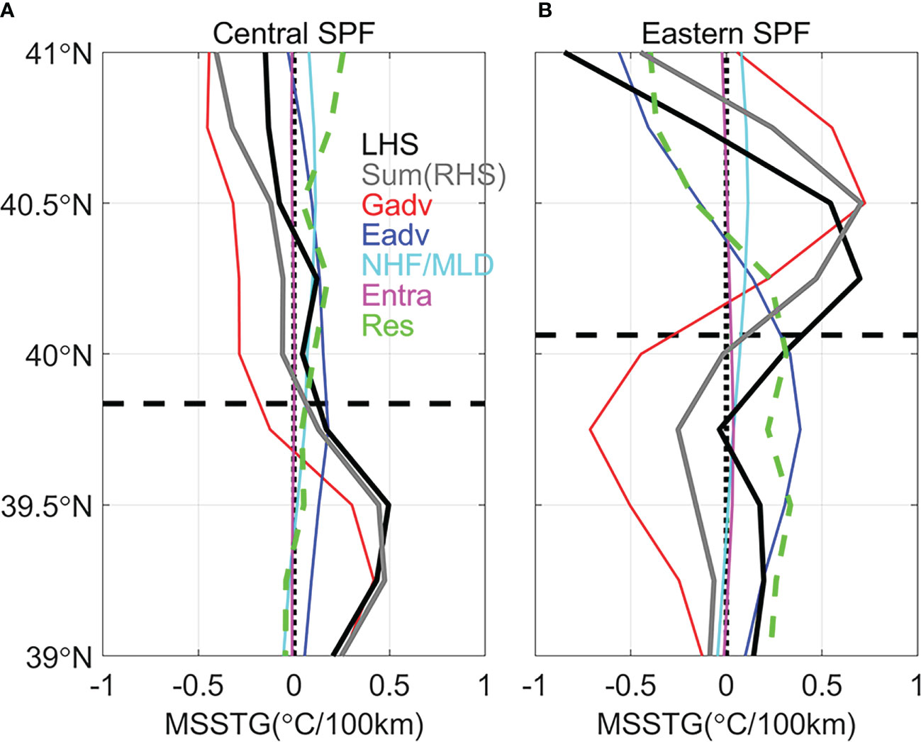
Figure 5 Zonal averaged decadal change in the MSSTG between 1993–2002 and 2011–2020 (the latter minus the former; unit: °C/100km) calculated by the frontogenesis rate equation for (A) 130–135°E (central SPF) and (B) 135–138°E (eastern SPF). Black horizontal dashed lines represent main axis position of the SPF. Black vertical dashed lines represent 0 value. Black thick solid lines indicate the results of the frontogenesis rate term [the LHS of equation (3)]. Red, blue, cyan and magenta solid lines represent the geostrophic advection (Gadv), Ekman advection (Eadv), NHF/MLD and entrainment (Entra) terms, respectively. Gray thick solid lines indicate the sum of the RHS of equation (3) (sum of Gadv, Eadv, MHF/MLD and Entra). Green thick dashed lines (Res) represent differences between the LHS and RHS of equation (3).

4.2 Contributions from geostrophic advection

We estimated the zonal and meridional components of the horizontal geostrophic advection term to further investigate the contributions of geostrophic advection (Figures 6A, C). The zonal geostrophic advection makes a large contribution to the intensification and meridional movements of the central and eastern SPF. Based on equation (6), the zonal geostrophic advection can be decomposed into the zonal shear advection and the zonal advection of the MSSTG, respectively (Figures 6B, D).

FIGURE 6

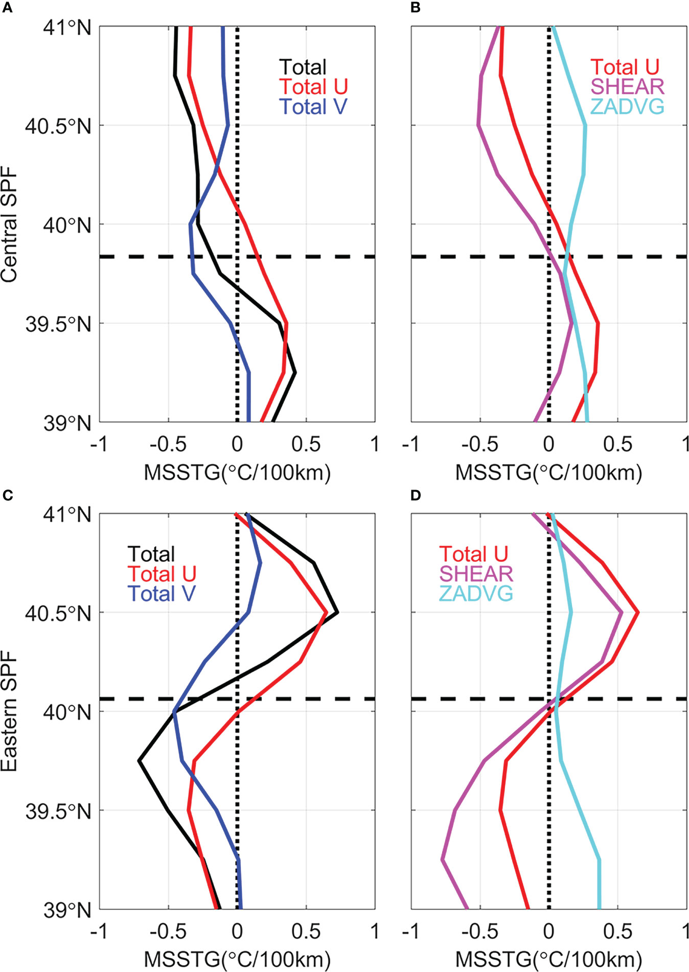
Figure 6 Zonal averaged decadal change in the MSSTG between 1993–2002 and 2011–2020 (the latter minus the former; unit: °C/100km) caused by the geostrophic advection term for (A, B) 130–135°E (central SPF) and (C, D) 135–138°E (eastern SPF). Black horizontal dashed lines represent main axis position of the SPF. Black vertical dashed lines represent 0 value. Black, red, blue, magenta and cyan solid lines indicate the decadal change in the MSSTG caused by the total geostrophic advection gradient term (Total), total zonal geostrophic advection gradient term (Total U), total meridional geostrophic advection gradient term (Total V), zonal shear advection term (SHEAR) and zonal advection of the MSSTG term (ZADVG).

In the central SPF, the zonal shear advection weakens the MSSTG over the polar flank. By contrast, the zonal advection of the MSSTG enhances the MSSTG over the equatorial flank of the central SPF and partly offsets the decrease induced by the zonal shear advection. The zonal advection of the MSSTG represents the transport of the MSSTG by zonal geostrophic current. Figure 7B shows the decadal changes in the zonal geostrophic current. The zonal geostrophic current is enhanced on the equatorial side of the central SPF. The intensified eastward current results in stronger MSSTG advection along the central SPF on the equatorial side. Figure 8 shows the climatological horizontal geostrophic current fields during the time period 1993–2020 and the decadal changes between 1993–2002 and 2011–2020 (the latter minus the former). Yabe et al. (2021) reported that the SPF Current (SFC) turns to flow eastward at about 40°N. This implies that the SFC has strengthened in the upstream region over the past decades, resulting in stronger MSSTG advection (Figure 8B). The zonal shear advection represents the conversion of the zonal SST gradient into the MSSTG via zonal current shear. As shown in Figures 7A, B and Figure 8B, the SFC has weakened in the polar flank of the central SPF, which induces negative zonal shear. The negative zonal shear causes the cold temperature advection to weaken poleward on the polar flank of the central SPF, which, in turn, induces weakening of the MSSTG.

FIGURE 7

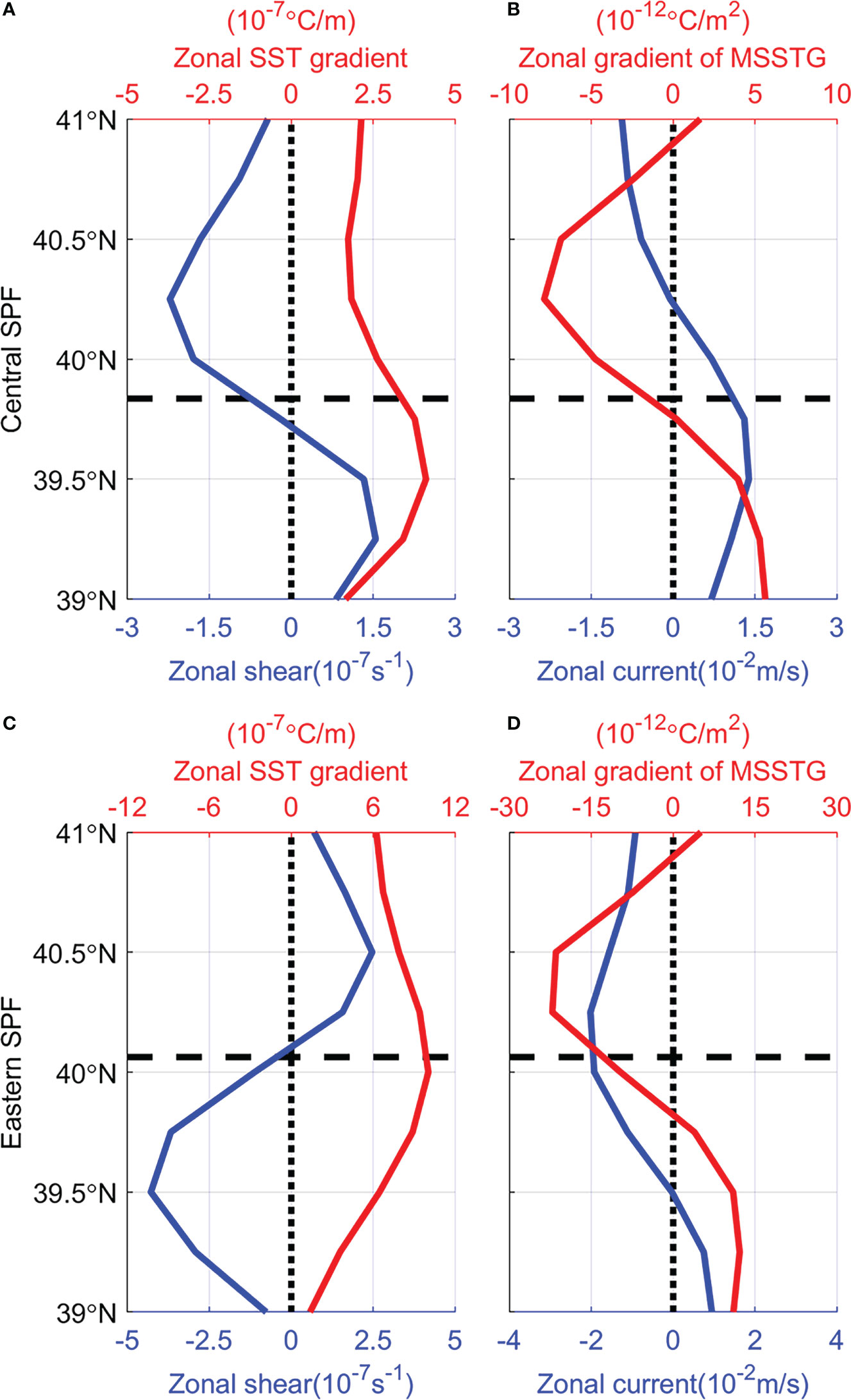
Figure 7 (A) Zonal averaged decadal change in the zonal geostrophic shear (blue solid line; unit: 10^-7s^-1) and zonal SST gradient (red solid line; unit: 10^-7°C/m) for the central SPF. (B) Same as (A) but for the zonal geostrophic current (blue solid line; unit: 10^-2m/s) and the zonal gradient of the MSSTG (red solid line; unit: 10^-12°C/m²). Black dashed lines represent the zonal averaged position of the central SPF. (C, D) Same as (A, B) but for the eastern SPF.

FIGURE 8

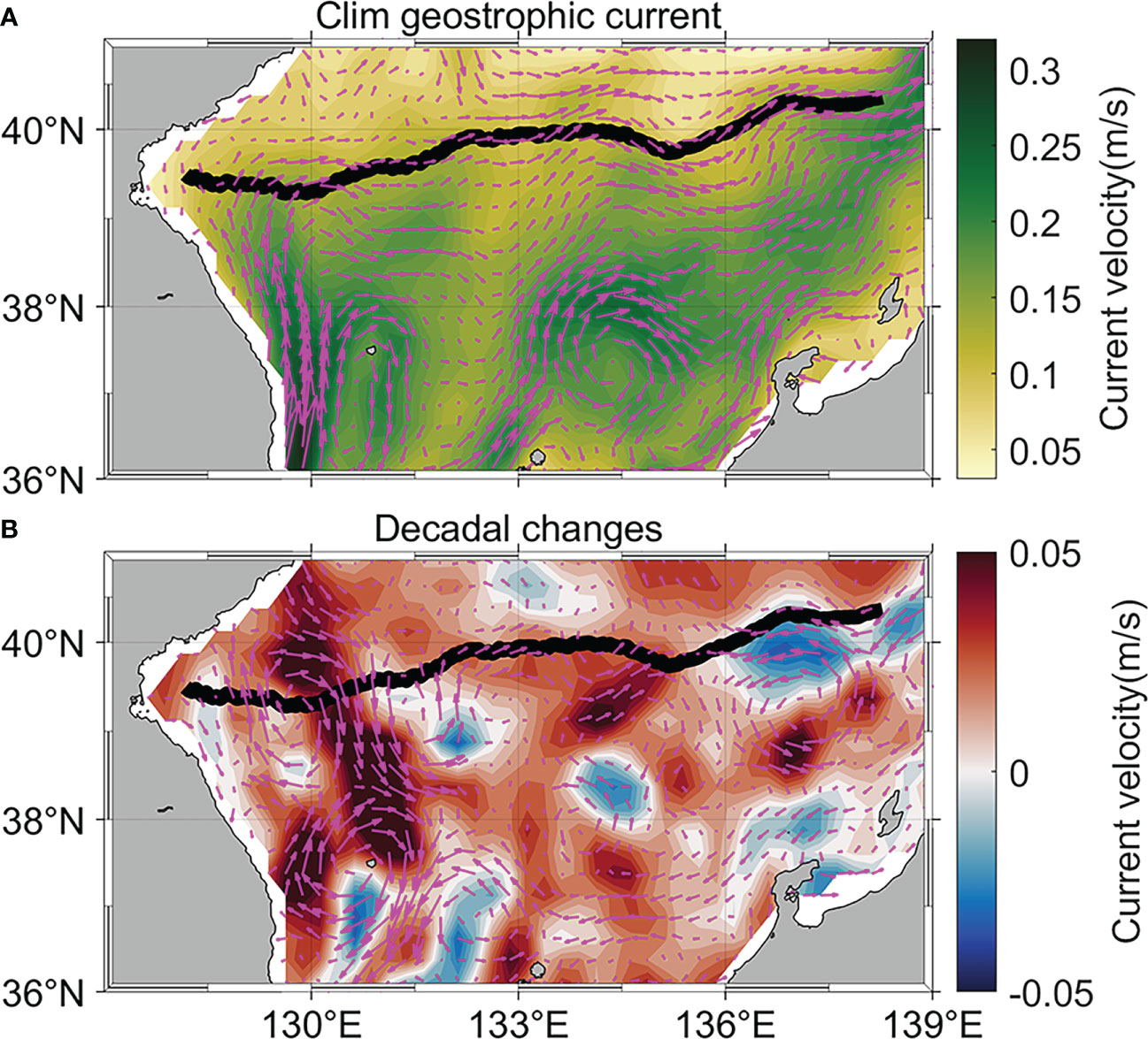
Figure 8 (A) Climatological horizontal geostrophic current velocity (color; unit: m/s) and vector during the time period of 1993–2020. (B) Decadal change of geostrophic current in the time periods 1993–2002 and 2011–2020 (the latter minus the former; unit: m/s).

Figure 6D shows the zonal shear advection and the zonal advection of the MSSTG over the two sides of the eastern SPF. The change in the MSSTG induced by zonal shear advection makes the dominant contribution to the poleward intensification and movement of the eastern SPF. There is a broad westward current anomaly in the region between 39.5 and 41°N, in contrast with the eastward SFC, which induces a weaker SFC and a meander on the downstream of the SFC (Figure 7D). The weakening of the SFC results in positive (negative) zonal shear over the polar (equatorial) flanks of the eastern SPF (Figure 7C). The zonal shear results in weak cold temperature advection near the eastern SPF and strong cold temperature advection on both sides of the polar and equatorial flanks, which increases (decreases) the MSSTG on the polar (equatorial) flanks.

The variation of geostrophic current is also revealed in the decadal changes in the SLA (Figure 9A). Over the equatorial side of the central SPF, the SLA is higher, associated with the eastward current, which contributes to the acceleration of the current system around the central SPF. The change in the SLA due to non-steric effect appears to be well following the higher (lower) SLA over the equatorial (polar) flanks of the central SPF (Figure 9C), but the decadal change due to the steric effect is relatively weak compared to η^′ and ${\eta }_{Nonsteric}^{\text{'}}$, and does not show a pattern that contributes to the acceleration of geostrophic current (Figure 10B). This is consistent with the results pointed out by previous studies that the non-steric effect plays a more important role in decadal, interannual and longer timescales than the steric effect (Yoon et al., 2016; Jeong et al., 2022). Moreover, the non-steric effect is affected by the volume transport from the upstream. As shown in Figure 8A, one branch of the TWC originating from the west channel of the KTS and flowed poleward along the Korean Peninsula, namely East Korea Warm Current (EKWC, Yoon and Kim (2009)), while the SFC is an extension of the EKWC at about 39-40°N (Yabe et al., 2021). Figure 8B shows the acceleration of the EKWC. Besides, recent studies reported an intensified throughflow transport in the KTS (Kida et al., 2021; Shin et al., 2022), suggesting that the increased intrusion across the KTS can cause the non-steric effect. Shin et al. (2022) reported that the volume transport increased 0.14 Sv (1Sv=10⁶m³/s) in the west channel of the KTS during the time period 1989–2018, which is comparable to the magnitude of the change in the geostrophic current. Thus, the intensified volume transport across the KTS induces the higher SLA in the upstream region, leading to the acceleration of the SFC. According to the previous studies, the intensified volume transport in the KTS may be induced by the decreasing of the transport of Kuroshio and the poleward movement of the Kuroshio axis (Kida et al., 2021; Shin et al., 2022; Usui and Ogawa, 2022), which further implies that the variability in open ocean affects the marginal sea through the KTS. Moreover, the SFC is locally affected by the topographic features, which may be responsible for the meander of the SFC in the downstream region (Yabe et al., 2021).

FIGURE 9

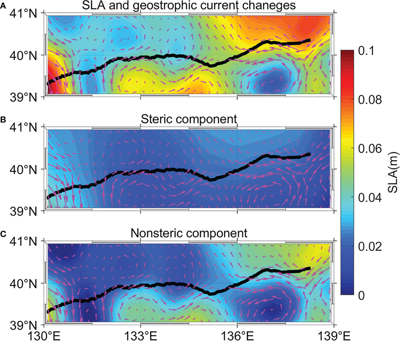
Figure 9 (A) Decadal change in the SLA between the time periods 1993–2002 and 2011–2020 (the latter minus the former; shading: SLA, unit: m). (B, C) Same as (A) but for the results of steric and non-steric components. Magenta vectors are the geostrophic currents decadal changes, duplicated from Figure 8B.

The decomposition described in this subsection again shows that geostrophic advection, which is controlled by the SFC, dominates the intensification and slant of the SPF. The zonal advection of the MSSTG associated with the increase in the SFC in the upstream region is responsible for the intensification and equatorward movement of the central SPF, whereas the intensification and poleward movement of the eastern SPF is dominated by zonal shear advection controlled by the zonal shear of the SFC in the downstream region.

4.3 Impact of Ekman advection on the different shift trends in the eastern SPF before and after 2002

There was a decadal shift in the eastern SPF before and after 2002 (Figure 3F). To determine the underlying mechanisms, we calculated the results of different mechanisms using the frontogenesis rate equation (Figures 10A, G). Before 2002, the MSSTG intensified over the polar flank of the eastern SPF and weakened over its equatorial flank (Figure 10A). However, after 2002, the MSSTG showed consistent intensification over the polar and equatorial sides of the eastern SPF (Figure 10G). The geostrophic and Ekman currents had different roles. The geostrophic advection showed similar effects both before and after 2002, which increased (decreased) the MSSTG over the polar (equatorial) sides of the eastern SPF (Figures 10C, I), whereas the Ekman advection was almost the opposite before and after 2002 (Figures 10B, H). Before 2002, the effects of the Ekman advection were similar to those of the geostrophic advection, strengthening (weakening) the MSSTG over the polar (equatorial) sides of the eastern SPF. By contrast, after 2002, the Ekman advection had the opposite role in the polar and equatorial flanks. Besides, the decadal changes in the MSSTG induced by the NHF/MLD, entrainment and residual terms are small (Figures 10D–F, J–L). The different decadal changes in the shift of the eastern SPF can therefore be attributed to the opposite changes in the Ekman advection before and after 2002.

FIGURE 10

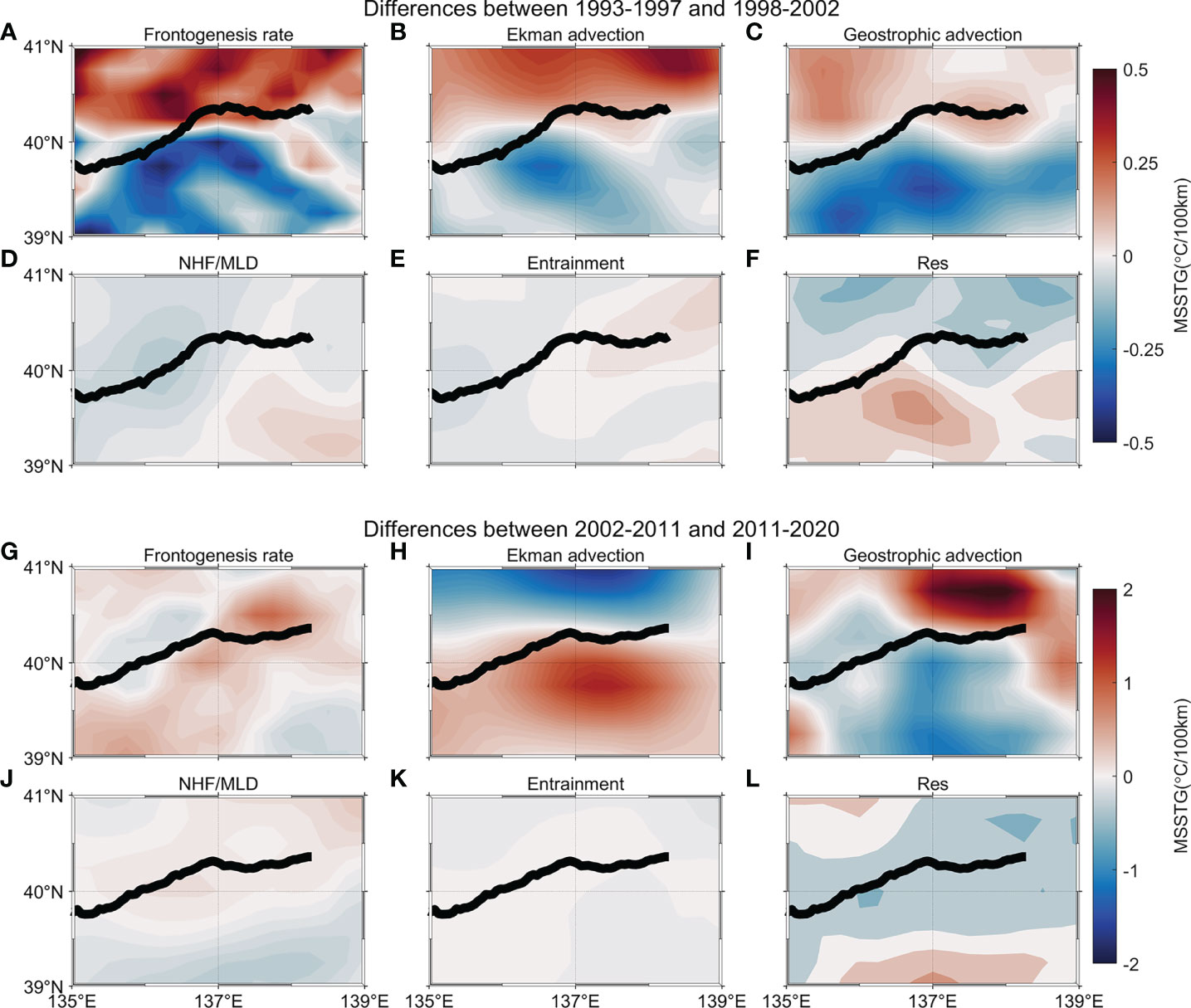
Figure 10 (A) Decadal change in the MSSTG between the time periods 1993–1997 and 1998–2002 (the latter minus the former; unit: °C/100km) calculated from the frontogenesis rate term. (C–F) Same as (A) but for the decadal change in the MSTTG calculated by (B) the Ekman advection gradient term, (C) the geostrophic advection gradient term, (D) the NHF/MLD gradient term, (E) the entrainment gradient term and (F) the differences between the LHS and RHS of equation (3). Black solid lines represent the mean position of the SPF during the time period 1993–2002. (G–L) Same as (A–F) but for the changes between the time periods 2002–2011 and 2011–2020 (the latter minus the former; unit: °C/100km) and the mean position of the SPF during the time period 2002–2020.

The Ekman advection was further separated into zonal and meridional components (Figures 11A, B, F, G). The meridional Ekman advection made a large contribution to the decadal changes in the MSSTG before and after 2002. Based on equation (6), the meridional Ekman advection can be decomposed into meridional convergence advection and meridional advection of the MSSTG, which indicate that the decadal changes in the MSSTG were caused by the convergence or divergence of the meridional current and the transport of the MSSTG by the meridional current, respectively (Figures 11C, D, H, I).

FIGURE 11

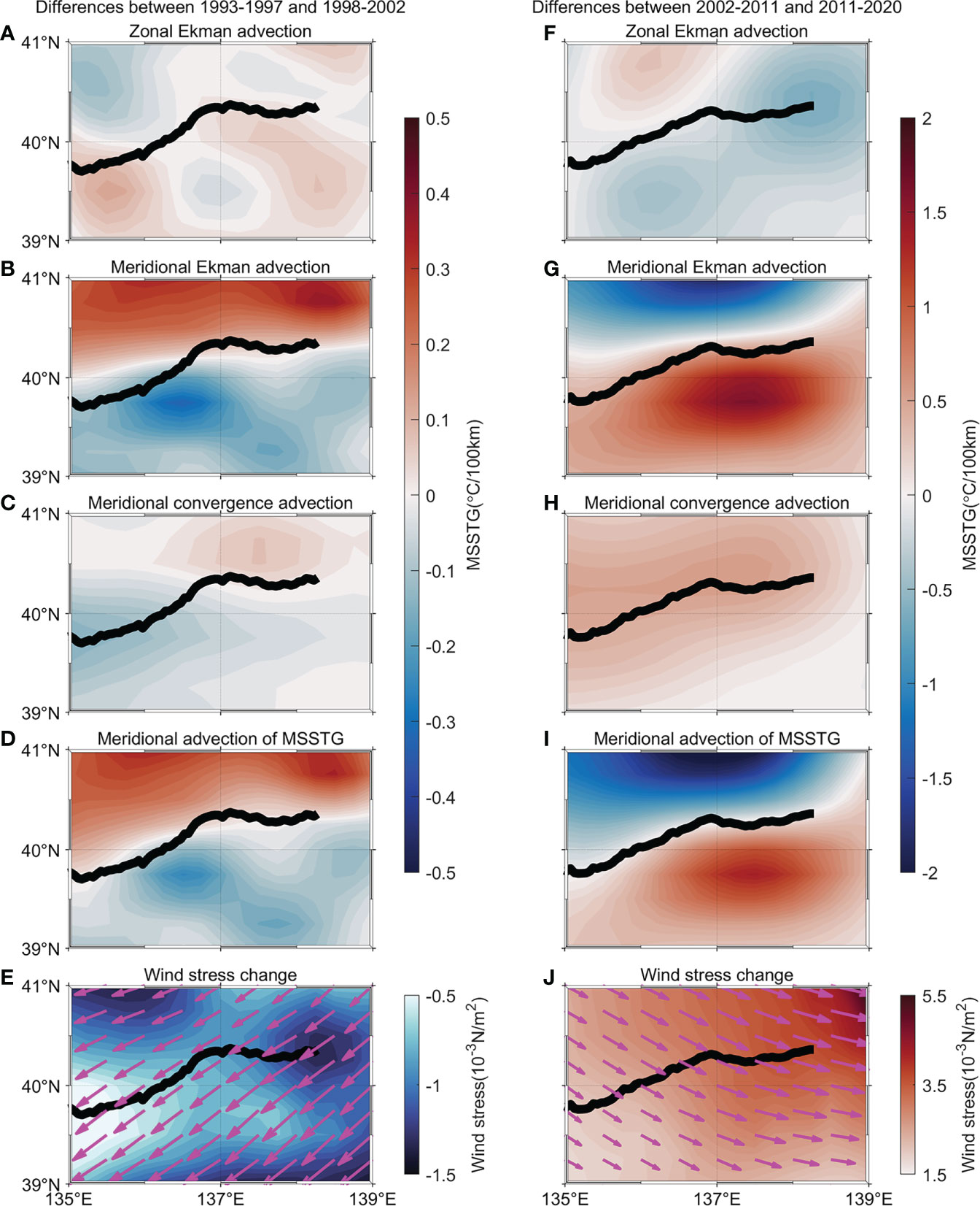
Figure 11 (A) Decadal change in the MSSTG between the time periods 1993–1997 and 1998–2002 (the latter minus the former; unit: °C/100km) caused by the total zonal Ekman advection gradient term. (B–D) Same as (A) but for the decadal change in the MSSTG caused by the total meridional Ekman advection gradient term in (B), meridional convergence advection term in (C) and meridional advection of the MSSTG term in (D). (E) The decadal change in the wind stress in the time periods 1993–1997 and 1998–2002 (the latter minus the former; color: wind stress magnitude; vectors: horizontal wind stress vectors; unit: 10^-3N/m²). Black solid lines represent the mean position of the SPF during the time period 1993–2002. (F–J) Same as (A–E) but for the changes in the time periods 2002–2011 and 2011–2020 (the latter minus the former; unit: °C/100km and 10^-3N/m²) and the mean position of the SPF during the time period 2002–2020.

We have shown that the meridional advection of the MSSTG mostly controls the Ekman advection and is much more important than the meridional convergence advection. Hence there may be a decadal shift in the large-scale wind field. The decadal changes in the wind stress before and after 2002 are shown in Figures 11E, J. Before 2002, an easterly wind stress anomaly caused the poleward transport of the MSSTG, which strengthened (weakened) the MSSTG over the polar (equatorial) flanks of the eastern SPF (Figures 11D, E). By contrast, after 2002, the equatorward transport of the MSSTG induced by the westerly wind stress anomaly resulted in the opposite changes in the MSSTG on the polar and equatorial sides of the eastern SPF (Figures 11I, J).

The zonal wind stress anomaly is the key point for the changes in Ekman advection both before and after 2002. Figure 12A shows the zonal wind stress anomaly averaged in the JES. Before 2002, there was a shift from a westerly anomaly to an easterly anomaly, and vice versa after 2002. The wind stress field in the JES is related to the large-scale East Asian Winter Monsoon (EAWM), which revealed by the sea-level pressure (SLP) in the region of Siberian High (SH) and in East Asia (Ding et al., 2014; Jeong et al., 2022). An intensity index of EAWM (hereinafter EAWM index) is defined as the sum of winter (winter is the average of December, January, and February) zonal SLP differences (110°E minus 160°E) over 20–70°N following Wu and Wang (2002). Note that the index calculated by the annual SLP differences is well correlated with the EAWM index (correlation coefficient 0.72 at 99% confidence level in decadal timescales), the latter one is employed to represent the atmospheric forcing field. Figure 12B shows the decadal time series of EAWM index. The EAWM index and the zonal wind stress anomaly are positively correlated (correlation coefficient 0.54) at the 95% confidence level. The EAWM index has weakened before early 2000s and gradually increased after early 2000s, indicative of a decadal difference in EAWM before and after early 2000s, which is consistent with previous studies (He, 2013; Ding et al., 2014). Spatial patterns in SLP and wind stress decadal changes before and after early 2000s are shown in Figures 12C, D. The EAWM weakened (strengthened) before (after) 2002, leading to the changes in the easterly (westerly) wind stress anomaly. Previous studies indicated that the EAWM has been significantly affected by global climate change, the major atmospheric pattern in Northern Hemisphere (NH) and the Pacific SST in decadal timescale (Gong et al., 2001; Wu and Wang, 2002; Wang et al., 2008; He, 2013; Ding et al., 2014). The time period before early 2000s was so-called “fast warming”, while the following decade was the global warming “hiatus” (Deser et al., 2017). For the atmospheric factor, the Arctic Oscillation, which is the dominant mode of extratropical climate variation of the NH, can influence the EAWM through altering the large-scale circulation over Eurasia and the strength of the NH (Gong et al., 2001; Liu et al., 2017). For the oceanic factor, the Pacific Decadal Oscillation is well related to the overlaying Aleutian Low and the circulation over Eurasia (Chhak et al., 2009; Ding et al., 2014).

FIGURE 12

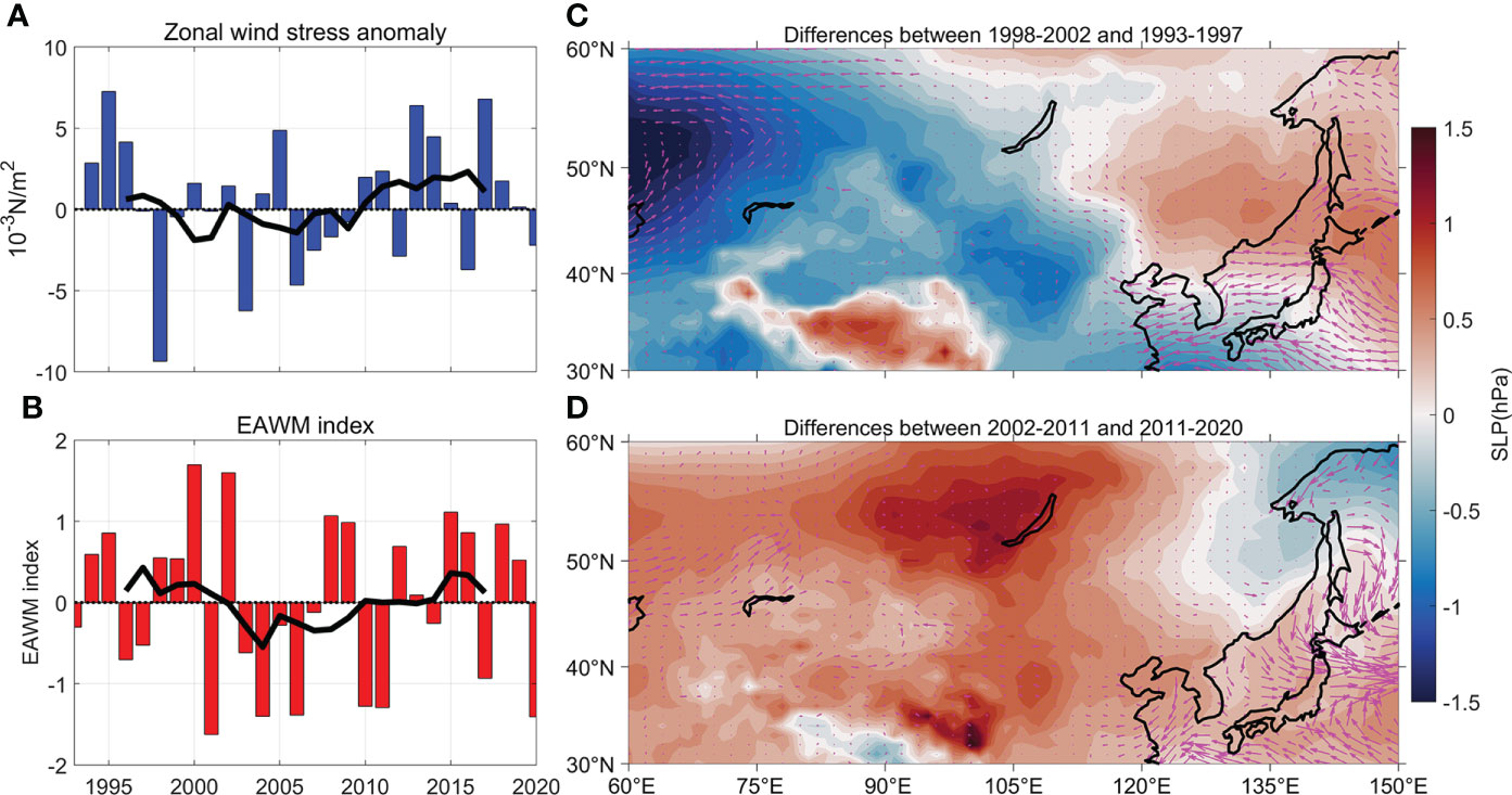
Figure 12 (A) Time series of basin-averaged zonal wind stress anomaly (unit: N/m²) for the annual mean (blue bars) and seven-year running averages (black solid line). (B) Same as (A) but for the time series of EAWM index. (C) Decadal change in the SLP and wind stress vectors between the time periods 1993–1997 and 1998–2002 (the latter minus the former; unit: hPa and N/m²). (D) Same as (C) but for the change in the time periods 2002–2011 and 2011–2020.

5 Summary

In this study, the decadal trends of the SPF in the JES during the time period 1985–2020 using four high-resolution satellite-observed SST products was investigated. All the datasets showed consistent intensification and poleward (equatorward) shifts in the eastern (central) SPF. The results of our analysis indicated that the meridional movements of the SPF were associated with the increase in the MSSTG over the polar (equatorial) flanks of the eastern (central) SPF and weakening of the MSSTG over the equatorial (polar) flanks of the eastern (central) SPF. The SPF is slanted more to the southwest–northeast as a result of the opposite meridional movements of the central and eastern SPF. We explored the possible mechanisms using the frontogenesis rate equation, which showed that the geostrophic advection term had a dominant role. Further analyses of the geostrophic advection term indicated that the poleward intensification and shift in the eastern SPF were caused by zonal shear advection. The equatorward intensification and movement of the central SPF were determined by the zonal advection of the MSSTG. For the eastern SPF, the shear of the SFC in the downstream region had a dominant role, whereas the equatorward enhancement in the upstream region was important for the central SPF. And the intensified volume transport across the KTS may contribute to the acceleration of the SFC. Figure 13 shows a schematic diagram of the decadal trend of the SPF.

FIGURE 13

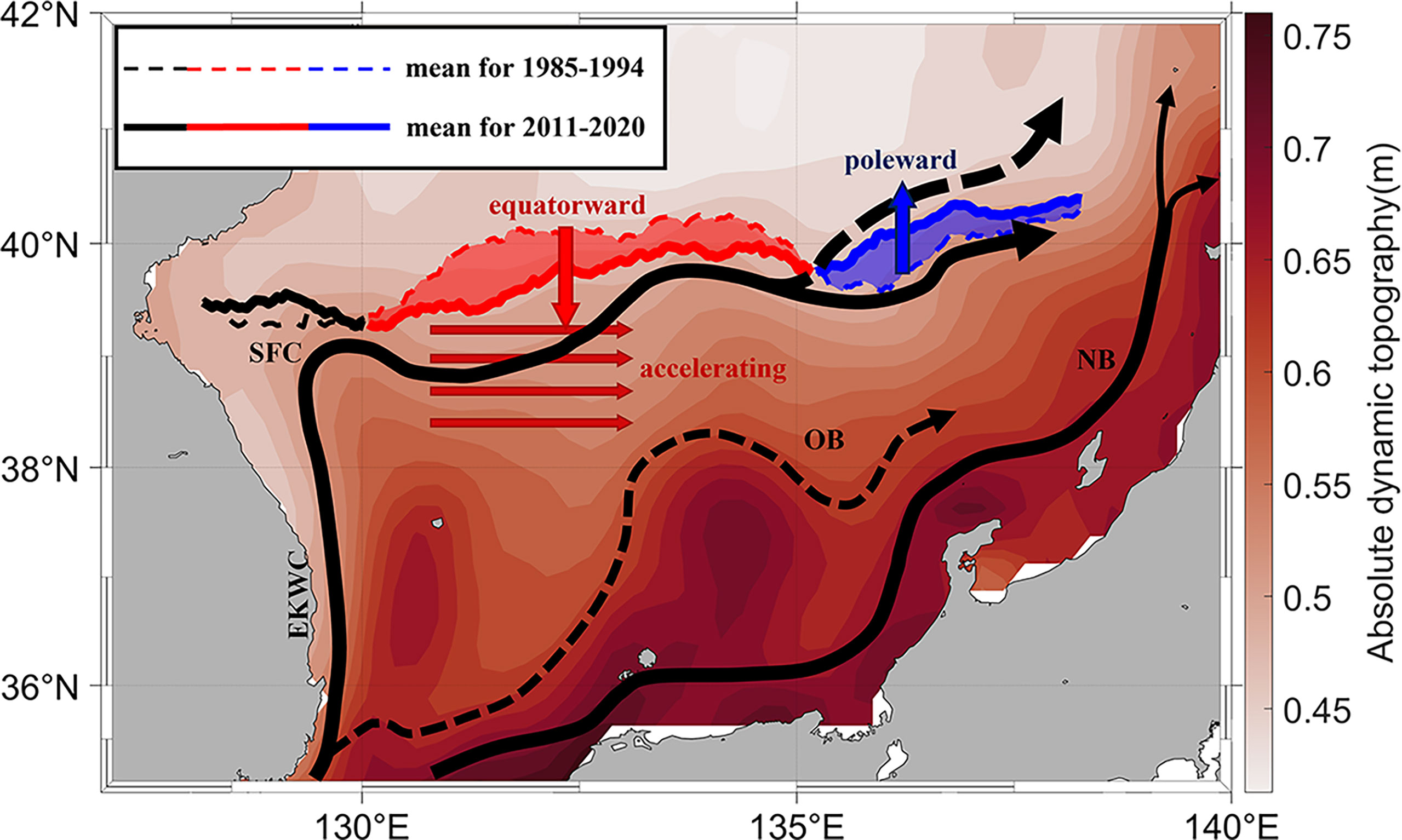
Figure 13 Schematic of the slantwise SPF in the JES. The average positions in the time periods 2011–2020 and 1985–1994 are denoted by the solid and dashed lines, respectively. The SPF is slanted more to the southwest-northeast as a result of the opposite meridional movements of the central and eastern SPF. The black, red and blue solid (dashed) lines are the western, central and eastern SPF, respectively. The shaded regions between the two lines are the meridional movements between the two decades. The black arrows denote the TWC. EKWC: East Korea Current, OB: offshore branch, NB: nearshore branch, TWC: Tsushima Warm Current, SFC: Subpolar Front Current. Red shading is climatological absolute dynamics topography (unit: m).

Previous numerical experiments indicated that both the local and remote atmospheric conditions were sensitive to changes in the JES SST, including the surface winds, precipitation, and the regional and large-scale atmospheric circulations (Yamamoto and Hirose, 2008; Yamamoto and Hirose, 2009; Yamamoto and Hirose, 2011; Seo et al., 2014). The changes in the intensity and position of the SPF may profoundly influence the overlying atmosphere and passing extratropical cyclones (Yoshiike and Kawamura, 2009; Yamamoto, 2013). Winter extratropical cyclones develop rapidly over the JES and enter into the northwestern Pacific (Zhao et al., 2016; Zhao et al., 2018). The decadal trend of the SPF in the JES may have far-reaching influences on the weather over Japan and the northwestern Pacific Ocean.

Data availability statement

Publicly available datasets were analyzed in this study. The CoralTemp data can be available at https://pae-paha.pacioos.hawaii.edu/erddap/griddap/dhw_5km.html. The OSTIA data was distributed by the Copernicus Marine and Environment Monitoring Service (https://resources.marine.copernicus.eu/product-detail/SST_GLO_SST_L4_REP_OBSERVATIONS_010_011/INFORMATION). ERA5 Reanalysis can be downloaded from https://cds.climate.copernicus.eu/cdsapp#!/dataset/reanalysis-era5-single-levels-monthly-means. Geostrophic surface currents and absolute dynamics topography can be downloaded from https://cds.climate.copernicus.eu/cdsapp#!/dataset/satellite-sea-level-global?tab=overview. ESASST data was downloaded from Copernicus climate data storge (https://cds.climate.copernicus.eu/cdsapp#!/dataset/satellite-sea-surface-temperature?tab=overview). The OISST data was accessed from https://www.ncdc.noaa.gov/oisst/optimum-interpolation-sea-surface-temperature-oisst-v21. EN4 data was accessed from https://hadleyserver.metoffice.gov.uk/en4/download-en4-2-2.html.

Author contributions

Conceptualization, SC and YCZ. Resources, YCZ. Data curation, SC and WC. Formal Analysis, SC, HW and YCZ. Supervision, YCZ. Investigation, WC and YZ. Visualization, SC. Methodology, SC, HW and YCZ. Writing – original draft, SC. Project administration, YCZ. Writing – review & editing, SC, HW, WC, YZ and YCZ. All authors contributed to the article and approved the submitted version.

Funding

The present study is supported by the National Key Research Program of China (2017YFA0604100). YCZ acknowledges support from National Natural Science Foundation of China (Grant No. 41406003), China Postdoctoral Science Foundation funded project (Grant No. 2013M541959), and Jiangsu Provincial Natural Science Foundation (Grant No. BK20130064). HW acknowledges support from National Natural Science Foundation of China (42276205).

Conflict of interest

The authors declare that the research was conducted in the absence of any commercial or financial relationships that could be construed as a potential conflict of interest.

Publisher’s note

All claims expressed in this article are solely those of the authors and do not necessarily represent those of their affiliated organizations, or those of the publisher, the editors and the reviewers. Any product that may be evaluated in this article, or claim that may be made by its manufacturer, is not guaranteed or endorsed by the publisher.

Supplementary material

The Supplementary Material for this article can be found online at: https://www.frontiersin.org/articles/10.3389/fmars.2022.1038024/full#supplementary-material

References

Akima H. (1970). A new method of interpolation and smooth curve fitting based on local procedures. J. ACM 17 (4), 589–602. doi: 10.1145/321607.321609

CrossRef Full Text | Google Scholar

Chang K.-I., Zhang C.-I., Park C., Kang D.-J., Ju S.-J., Lee S.-H., et al. (2016). Oceanography of the East Sea (Japan Sea) (Cham: Springer).

Google Scholar

Chen S., Wang H., Wang N., Wang H., Yu P., Yang X., et al. (2022). Dominant modes of winter SST variability in the Japan Sea and their influences on atmosphere. J. Oceanogr. 78 (5), 353–368. doi: 10.1007/s10872-022-00643-8

CrossRef Full Text | Google Scholar

Chhak K. C., Di Lorenzo E., Schneider N., Cummins P. F. (2009). Forcing of low-frequency ocean variability in the northeast pacific. J. Clim. 22 (5), 1255–1276. doi: 10.1175/2008JCLI2639.1

CrossRef Full Text | Google Scholar

Choi B.-J., Haidvogel D. B., Cho Y.-K. (2009). Interannual variation of the polar front in the Japan/East Sea from summertime hydrography and sea level data. J. Mar. Syst. 78 (3), 351–362. doi: 10.1016/j.jmarsys.2008.11.021

CrossRef Full Text | Google Scholar

Deser C., Guo R., Lehner F. (2017). The relative contributions of tropical pacific sea surface temperatures and atmospheric internal variability to the recent global warming hiatus. Geophys. Res. Lett. 44 (15), 7945–7954. doi: 10.1002/2017GL074273

CrossRef Full Text | Google Scholar

Ding Y., Liu Y., Liang S., Ma X., Zhang Y., Si D., et al. (2014). Interdecadal variability of the East Asian winter monsoon and its possible links to global climate change. J. Meteorol. Res. 28 (5), 693–713. doi: 10.1007/s13351-014-4046-y

CrossRef Full Text | Google Scholar

Frankignoul C., de Coëtlogon G., Joyce T. M., Dong S. (2001). Gulf stream variability and ocean–atmosphere interactions. J. Phys. Oceanogr. 31 (12), 3516–3529. doi: 10.1175/1520-0485(2002)031<3516:GSVAOA>2.0.CO;2

CrossRef Full Text | Google Scholar

Gill A. E., Niller P. P. (1973). The theory of the seasonal variability in the ocean. Deep-Sea Res. Oceanogr. Abstr. 20 (2), 141–177. doi: 10.1016/0011-7471(73)90049-1

CrossRef Full Text | Google Scholar

Gong D.-Y., Wang S.-W., Zhu J.-H. (2001). East Asian Winter monsoon and Arctic oscillation. Geophys. Res. Lett. 28 (10), 2073–2076. doi: 10.1029/2000GL012311

CrossRef Full Text | Google Scholar

Good S., Fiedler E., Mao C., Martin M. J., Maycock A., Reid R., et al. (2020). The current configuration of the OSTIA system for operational production of foundation Sea surface temperature and ice concentration analyses. Remote Sens. 12 (4), 720. doi: 10.3390/rs12040720

CrossRef Full Text | Google Scholar

Gouretski V., Reseghetti F. (2010). On depth and temperature biases in bathythermograph data: Development of a new correction scheme based on analysis of a global ocean database. Deep. Res. Part I Oceanogr. Res. Pap. 57 (6), 812–833. doi: 10.1016/j.dsr.2010.03.011

CrossRef Full Text | Google Scholar

He S. (2013). Reduction of the East Asian winter monsoon interannual variability after the mid-1980s and possible cause. Chin. Sci. Bull. 58 (12), 1331–1338. doi: 10.1007/s11434-012-5468-5

CrossRef Full Text | Google Scholar

Hersbach H., Bell B., Berrisford P., Hirahara S., Horányi A., Muñoz-Sabater J., et al. (2019). The ERA5 global reanalysis. Q. J. R. Meteorol. Soc. 146 (730), 1999–2049. doi: 10.1002/qj.3803

CrossRef Full Text | Google Scholar

Huang B., Liu C., Banzon V., Freeman E., Graham G., Hankins B., et al. (2021). Improvements of the daily optimum interpolation Sea surface temperature (DOISST) version 2.1. J. Clim. 34 (8), 2923–2939. doi: 10.1175/jcli-d-20-0166.1

CrossRef Full Text | Google Scholar

Huh O. K. (1982). Spring season flow of the tsushima current and its separation from the kuroshio: Satellite evidence. J. Geophys. Res.: Oceans 87 (C12), 9687–9693. doi: 10.1029/JC087iC12p09687

CrossRef Full Text | Google Scholar

Jeong Y., Nam S., Kwon J.-I., Uppara U., Jo Y.-H. (2022). Surface warming slowdown with continued subsurface warming in the East Sea (Japan Sea) over recent decade (2000–2014). Front. Mar. Sci. 9. doi: 10.3389/fmars.2022.825368

PubMed Abstract | CrossRef Full Text | Google Scholar

Joyce T. M., Deser C., Spall M. A. (2000). The relation between decadal variability of subtropical mode water and the north Atlantic oscillation. J. Clim. 13 (14), 2550–2569. doi: 10.1175/1520-0442(2000)013<2550:Trbdvo>2.0.Co;2

CrossRef Full Text | Google Scholar

Kida S., Mitsudera H., Aoki S., Guo X., Ito S.-I., Kobashi F., et al. (2015). Oceanic fronts and jets around Japan: a review. J. Oceanogr. 71 (5), 469–497. doi: 10.1007/s10872-015-0283-7

CrossRef Full Text | Google Scholar

Kida S., Takayama K., Sasaki Y. N., Matsuura H., Hirose N. (2021). Increasing trend in Japan Sea throughflow transport. J. Oceanogr. 77 (1), 145–153. doi: 10.1007/s10872-020-00563-5

CrossRef Full Text | Google Scholar

Kwon Y.-O., Alexander M. A., Bond N. A., Frankignoul C., Nakamura H., Qiu B., et al. (2010). Role of the gulf stream and kuroshio–oyashio systems in Large-scale atmosphere–ocean interaction: A review. J. Clim. 23 (12), 3249–3281. doi: 10.1175/2010jcli3343.1

CrossRef Full Text | Google Scholar

Large W. G., Pond S. (1981). Open ocean momentum flux measurements in moderate to strong winds. J. Phys. Oceanogr. 11 (3), 324–336. doi: 10.1175/1520-0485(1981)011<0324:OOMFMI>2.0.CO;2

CrossRef Full Text | Google Scholar

Lee E.-Y., Park K.-A. (2019). Change in the recent warming trend of Sea surface temperature in the East Sea (Sea of Japan) over decades, (1982–2018). Remote Sens. 11 (22), 2613. doi: 10.3390/rs11222613

CrossRef Full Text | Google Scholar

Legeckis R. (1978). A survey of worldwide sea surface temperature fronts detected by environmental satellites. J. Geophys. Res.: Oceans 83 (C9), 4501–4522. doi: 10.1029/JC083iC09p04501

CrossRef Full Text | Google Scholar

Lim S., Jang C. J., Oh I. S., Park J. (2012). Climatology of the mixed layer depth in the East/Japan Sea. J. Mar. Syst. 96-97, 1–14. doi: 10.1016/j.jmarsys.2012.01.003

CrossRef Full Text | Google Scholar

Liu Y., He S., Li F., Wang H., Zhu Y. (2017). Interdecadal change between the Arctic oscillation and East Asian climate during 1900–2015 winters. Int. J. Climatol. 37 (14), 4791–4802. doi: 10.1002/joc.5123

CrossRef Full Text | Google Scholar

McWilliams J. C. (2021). Oceanic frontogenesis. Annu. Rev. Mar. Sci. 13 (1), 227–253. doi: 10.1146/annurev-marine-032320-120725

CrossRef Full Text | Google Scholar

Merchant C. J., Embury O., Bulgin C. E., Block T., Corlett G. K., Fiedler E., et al. (2019). Satellite-based time-series of sea-surface temperature since 1981 for climate applications. Sci. Data. 6 (1), 223. doi: 10.1038/s41597-019-0236-x

PubMed Abstract | CrossRef Full Text | Google Scholar

Minobe S., Kuwano-Yoshida A., Komori N., Xie S.-P., Small R. J. (2008). Influence of the gulf stream on the troposphere. Nature 452 (7184), 206–209. doi: 10.1038/nature06690

PubMed Abstract | CrossRef Full Text | Google Scholar

Ogawa F., Nakamura H., Nishii K., Miyasaka T., Kuwano-Yoshida A. (2012). Dependence of the climatological axial latitudes of the tropospheric westerlies and storm tracks on the latitude of an extratropical oceanic front. Geophys. Res. Lett. 39 (5), L05804. doi: 10.1029/2011GL049922

CrossRef Full Text | Google Scholar

Ohishi S., Aiki H., Tozuka T., Cronin M. F. (2019). Frontolysis by surface heat flux in the eastern Japan Sea: importance of mixed layer depth. J. Oceanogr. 75 (3), 283–297. doi: 10.1007/s10872-018-0502-0

CrossRef Full Text | Google Scholar

Ou H.-W., Gordon A. (2002). Subduction along a midocean front and the generation of intrathermocline eddies: A theoretical study. J. Phys. Oceanogr. 32 (6), 1975–1986. doi: 10.1175/1520-0485(2002)032<1975:SAAMFA>2.0.CO;2

CrossRef Full Text | Google Scholar

Pak G., Park Y.-H., Vivier F., Bourdallé-Badie R., Garric G., Chang K.-I. (2017). Upper-ocean thermal variability controlled by ocean dynamics in the kuroshio-oyashio extension region. J. Geophys. Res.: Oceans 122 (2), 1154–1176. doi: 10.1002/2016JC012076

CrossRef Full Text | Google Scholar

Park K.-A., Chung J. Y., Kim K. (2004). Sea Surface temperature fronts in the East (Japan) Sea and temporal variations. Geophys. Res. Lett. 31 (7), L07304. doi: 10.1029/2004GL019424

CrossRef Full Text | Google Scholar

Park K.-A., Ullman D. S., Kim K., Yul Chung J., Kim K.-R. (2007). Spatial and temporal variability of satellite-observed subpolar front in the East/Japan Sea. Deep. Res. Part I Oceanogr. Res. Pap. 54 (4), 453–470. doi: 10.1016/j.dsr.2006.12.010

CrossRef Full Text | Google Scholar

Peña-Molino B., Joyce T. M. (2008). Variability in the slope water and its relation to the gulf stream path. Geophys. Res. Lett. 35 (3), L03606. doi: 10.1029/2007GL032183

CrossRef Full Text | Google Scholar

Qiu C., Kawamura H., Mao H., Wu J. (2014). Mechanisms of the disappearance of sea surface temperature fronts in the subtropical north pacific ocean. J. Geophys. Res.: Oceans 119 (7), 4389–4398. doi: 10.1002/2014JC010142

CrossRef Full Text | Google Scholar

Sasaki Y. N., Schneider N. (2011). Interannual to decadal gulf stream variability in an eddy-resolving ocean model. Ocean Model. Online 39 (3), 209–219. doi: 10.1016/j.ocemod.2011.04.004

CrossRef Full Text | Google Scholar

Seo H., Kwon Y.-O., Park J.-J. (2014). On the effect of the East/Japan Sea SST variability on the north pacific atmospheric circulation in a regional climate model. J. Geophys. Res.: Atmos. 119 (2), 418–444. doi: 10.1002/2013JD020523

CrossRef Full Text | Google Scholar

Shin H.-R., Lee J.-H., Kim C.-H., Yoon J.-H., Hirose N., Takikawa T., et al. (2022). Long-term variation in volume transport of the tsushima warm current estimated from ADCP current measurement and sea level differences in the Korea/Tsushima strait. J. Mar. Syst. 232, 103750. doi: 10.1016/j.jmarsys.2022.103750

CrossRef Full Text | Google Scholar

Skirving W., Marsh B., de la Cour J., Liu G., Harris A., Maturi E., et al. (2020). CoralTemp and the coral reef watch coral bleaching heat stress product suite version 3.1. Remote Sens. 12 (23), 3856. doi: 10.3390/rs12233856

CrossRef Full Text | Google Scholar

Takatama K., Minobe S., Inatsu M., Small R. J. (2015). Diagnostics for near-surface wind response to the gulf stream in a regional atmospheric model. J. Clim. 28 (1), 238–255. doi: 10.1175/JCLI-D-13-00668.1

CrossRef Full Text | Google Scholar

Usui N., Ogawa K. (2022). Sea Level variability along the Japanese coast forced by the kuroshio and its extension. J. Oceanogr. 78 (6), 515–527. doi: 10.1007/s10872-022-00657-2

CrossRef Full Text | Google Scholar

Wang L., Chen W., Huang R. (2008). Interdecadal modulation of PDO on the impact of ENSO on the east Asian winter monsoon. Geophys. Res. Lett. 35 (20), L20702. doi: 10.1029/2008GL035287

CrossRef Full Text | Google Scholar

Wu B., Lin X., Qiu B. (2018). Meridional shift of the oyashio extension front in the past 36 years. Geophys. Res. Lett. 45 (17), 9042–9048. doi: 10.1029/2018GL078433

CrossRef Full Text | Google Scholar

Wu B., Lin X., Qiu B. (2019). On the seasonal variability of the oyashio extension fronts. Clim. Dyn. 53 (11), 7011–7025. doi: 10.1007/s00382-019-04972-1

CrossRef Full Text | Google Scholar

Wu B., Lin X., Yu L. (2021). Poleward shift of the kuroshio extension front and its impact on the north pacific subtropical mode water in the recent decades. J. Phys. Oceanogr. 51 (2), 457–474. doi: 10.1175/JPO-D-20-0088.1

CrossRef Full Text | Google Scholar

Wu B., Wang J. (2002). Winter Arctic oscillation, Siberian high and East Asian winter monsoon. Geophys. Res. Lett. 29 (19), 3–1-3-4. doi: 10.1029/2002GL015373

CrossRef Full Text | Google Scholar

Xu L., Wang K., Wu B. (2021). Weakening and poleward shifting of the north pacific subtropical fronts from 1980 to 2018. J. Phys. Oceanogr. 52 (3), 399–417. doi: 10.1175/JPO-D-21-0170.1

CrossRef Full Text | Google Scholar

Yabe I., Kawaguchi Y., Wagawa T., Fujio S. (2021). Anatomical study of tsushima warm current system: Determination of principal pathways and its variation. Prog. Oceanogr. 194, 102590. doi: 10.1016/j.pocean.2021.102590

CrossRef Full Text | Google Scholar

Yamamoto M. (2013). Effects of a semienclosed ocean on extratropical cyclogenesis: The dynamical processes around the Japan Sea on 23–25 January 2008. J. Geophys. Res.: Atmos. 118 (18), 10,391–310,404. doi: 10.1002/jgrd.50802

CrossRef Full Text | Google Scholar

Yamamoto M., Hirose N. (2008). Influence of assimilated SST on regional atmospheric simulation: A case of a cold-air outbreak over the Japan Sea. Atmos. Sci. Lett. 9 (1), 13–17. doi: 10.1002/asl.164

CrossRef Full Text | Google Scholar

Yamamoto M., Hirose N. (2009). Regional atmospheric simulation of monthly precipitation using high-resolution SST obtained from an ocean assimilation model: Application to the wintertime Japan Sea. Mon. Weather Rev. 137 (7), 2164–2174. doi: 10.1175/2009MWR2488.1

CrossRef Full Text | Google Scholar

Yamamoto M., Hirose N. (2011). Possible modification of atmospheric circulation over the northwestern pacific induced by a small semi-enclosed ocean. Geophys. Res. Lett. 38 (3), L03804. doi: 10.1029/2010GL046214

CrossRef Full Text | Google Scholar

Yang H., Lohmann G., Krebs-Kanzow U., Ionita M., Shi X., Sidorenko D., et al. (2020a). Poleward shift of the major ocean gyres detected in a warming climate. Geophys. Res. Lett. 47 (5), e2019GL085868. doi: 10.1029/2019GL085868

CrossRef Full Text | Google Scholar

Yang H., Lohmann G., Lu J., Gowan E. J., Shi X., Liu J., et al. (2020b). Tropical expansion driven by poleward advancing midlatitude meridional temperature gradients. J. Geophys. Res.: Atmos. 125 (16), e2020JD033158. doi: 10.1029/2020JD033158

CrossRef Full Text | Google Scholar

Yang H., Lohmann G., Wei W., Dima M., Ionita M., Liu J. (2016). Intensification and poleward shift of subtropical western boundary currents in a warming climate. J. Geophys. Res.: Oceans 121 (7), 4928–4945. doi: 10.1002/2015JC011513

CrossRef Full Text | Google Scholar

Yoon S.-T., Chang K.-I., Na H., Minobe S. (2016). An east-west contrast of upper ocean heat content variation south of the subpolar front in the East/Japan Sea. J. Geophys. Res.: Oceans 121 (8), 6418–6443. doi: 10.1002/2016JC011891

CrossRef Full Text | Google Scholar

Yoon J.-H., Kim Y.-J. (2009). Review on the seasonal variation of the surface circulation in the Japan/East Sea. J. Mar. Syst. 78 (2), 226–236. doi: 10.1016/j.jmarsys.2009.03.003

CrossRef Full Text | Google Scholar

Yoshiike S., Kawamura R. (2009). Influence of wintertime large-scale circulation on the explosively developing cyclones over the western north pacific and their downstream effects. J. Geophys. Res.: Atmos 114 (D13), D13110. doi: 10.1029/2009JD011820

CrossRef Full Text | Google Scholar

Yoshikawa Y., Awaji T., Akitomo K. (1999). Formation and circulation processes of intermediate water in the Japan Sea. J. Phys. Oceanogr. 29 (8), 1701–1722. doi: 10.1175/1520-0485(1999)029<1701:FACPOI>2.0.CO;2

CrossRef Full Text | Google Scholar

Zhao N., Iwasaki S., Isobe A., Lien R.-C., Wang B. (2016). Intensification of the subpolar front in the Sea of Japan during winter cyclones. J. Geophys. Res.: Oceans 121 (4), 2253–2267. doi: 10.1002/2015JC011565

CrossRef Full Text | Google Scholar

Zhao N., Iwasaki S., Yamamoto M., Isobe A. (2018). Modulation of extratropical cyclones by previous cyclones via the Sea surface temperature anomaly over the Sea of Japan in winter. J. Geophys. Res.: Atmos. 123 (12), 6312–6330. doi: 10.1029/2017JD027503

CrossRef Full Text | Google Scholar

Zhao N., Manda A., Han Z. (2014). Frontogenesis and frontolysis of the subpolar front in the surface mixed layer of the Japan Sea. J. Geophys. Res.: Oceans 119 (2), 1498–1509. doi: 10.1002/2013JC009419

CrossRef Full Text | Google Scholar