Reconstruction of long-term sea-level data gaps of tide gauge records using a neural network operator

The coastal sea level is an important factor in understanding and clarifying the physical processes in coastal seas. However, missing values and outliers of the sea level that occur for various reasons often disrupt the continuity of its time series. General-purpose time-series analysis and prediction methods are not tolerant of missing values, which is why researchers have attempted to fill these gaps. The disadvantage of conventional time-series reconstruction techniques is the low accuracy when missed sea-level records are longer than the timescales of coastal processes. To solve this problem, we used an artificial neural network, which is a novel tool for creating multivariate and nonlinear regression equations. The trained neural network weight set was designed to enable long-term reconstruction of sea level by acting as a one-step prediction operator. In addition, a data assimilation technique was developed and adapted to ensure seamless continuity between predicted and observed sea-level records. The application of our newly developed method to 3-day gaps of seal level records at 16 tide gauge stations around the Korean peninsula confirms that it can successfully reconstruct missing values with root-mean-squared errors of 0.5–1.1 cm on average.

Introduction

Observing natural phenomena is the cornerstone for understanding their complex characteristics. Sea-level fluctuations, an ocean phenomenon, represent many physical ocean processes, such as tides, tsunamis, inverse barometric effects, mean sea-level changes, and wave set-up (Pugh and Woodworth, 2014). It is also used for data assimilation of ocean dynamic models and calibration of remote sensing data, and serves as an important indicator of global warming (Cane et al., 1996; Carton, 2005; Bosch et al., 2014; Cooley et al., 2022). In general, to understand and simulate geophysical fluid dynamic processes, long and reliable continuous sea-level records are required (Pappas et al., 2014). However, a common problem with sea-level observations is the presence of gaps caused by gauge defects or bad weather conditions. Moreover, these sporadic or continuous gaps were further amplified after applying data quality control procedures. These problems hinder the analysis of research and practical applications of most numerical models and statistical methods (e.g., spectral analysis, calibration (learning) algorithms, stochastic modeling, and downscaling) that malfunction with missing values (Pappas et al., 2014). In addition, since the state-of-the-art artificial neural network (ANN) model is trained by matrix calculation, it cannot be operated in case with gaps in the input data.

To fill in the missing values of the time series, previous studies have applied various interpolation methods. The simplest method is to use linear or spline interpolation or to use the weighted average value of both local and global data (Pappas et al., 2014). Interpolation using frequency bands and statistical methods, such as autoregressive moving average (ARMA) (Turki et al., 2015) and autoregressive integrated moving average (ARIMA) (Ren et al., 2022) have been applied. Cyclostationary empirical orthogonal functions (CSEOF) for the reconstruction of sea level have also been used (Hamlington et al., 2014; Cheon et al., 2018). In addition, ad hoc methodologies have been applied to fill these gaps (Shao et al., 2015). However, these methods have significant drawbacks: they can only use a single variable and/or have difficulty using both long- and short-period signals. The weakness of traditional interpolation methods is that ocean and atmospheric factors cannot be included in the reproducing procedure at sea level; hence, their performance cannot be guaranteed when the sea-level time series have a gap longer than the time scales of coastal processes.

Because the ANN, the novel technique, is suitable for a multivariable and nonlinear regression process, various factors and time series can be treated simultaneously for data gap filling. Therefore, in recent studies, ANN has drawn considerable attention as a technique for interpolation and estimation in many research fields (e.g., Wenzel and Schröter, 2010; Silva et al., 2018; Lu et al., 2019; Fourrier et al., 2020; Lee et al., 2020; Contractor and Roughan, 2021). In this study, we developed a sea-level interpolation technique using an ANN that utilizes sea-level data from nearby stations and oceanic and atmospheric data. We applied an LSTM layer (Hochreiter and Schmidhuber, 1997), which has been recently used in natural time-series research (Kim et al., 2020; Nardelli, 2020; Song et al., 2020; Zhang et al., 2020; Dogan et al., 2021; Adytia et al., 2022; Ren et al., 2022), to maximize the use of long-term time series as the input value.

Matrix computation is the basis of general supervised learning, and hence, the inability to flexibly cope with long-term missing data has been a limitation of studies. Furthermore, the design errors of an ANN result in a simple imitation of the immediately preceding (or before a specific cycle) value (Huang and Kuo, 2018; Kim et al., 2020; Dogan et al., 2021). These mimicked results show a phase that lags behind the observed values. One solution to this problem is to use an equivalent backcast network that acts as a time-stepping operator (Wenzel and Schröter, 2010). Using this concept, in this study, the stored weight set was operated as a one-step prediction operator, which solved the continuous gap filling issue for long-term missing data.

Korea, located in the northwest Pacific Ocean, is surrounded by seas on three land sides, and the properties of sea levels vary for each coast because they are influenced by various physical oceanic processes as well as distinctive topological characteristics. In particular, these properties are determined by the ratio of astronomical tides to residuals. The Yellow Sea, located on the west side of Korea, has an average depth of 44 m, and large tidal fluctuations dominate sea level variations. In the East Sea, the Korean Strait, which is the entrance of the flow into the basin, is narrow and shallow; therefore, sufficient tidal energy cannot be introduced. Consequently, the East Sea is largely affected by meteorological tides that are mainly caused by atmospheric pressure (e.g., Park and Watts, 2005). The South Sea of Korea and the seas around Jeju Island have intermediate characteristics compared to the previous two seas (KHOA, 2020). In this study, we focus on the reconstruction of residuals of sea level, typically dominated by meteorological tides, which are more difficult to predict than astronomical tides. Using an ANN, we developed a generalized method that can reconstruct long-term non-tidal sea-level records. Subsequently, the performance will be assessed by applying it to sea-level records along the eastern and southern coasts of Korea.

Data and methods

Data collection and preprocessing

Sea-level data and related atmospheric and oceanic data were collected from the tidal gauge stations of the Korea Hydrographic and Oceanographic Agency (KHOA) and automated synoptic observing system (ASOS) stations on land along the coast and ocean data buoys of the Korea Meteorological Administration (KMA). Sea-level data were obtained from 16 observation sites in three areas, as shown in Figure 1 and Table 1. The three areas were determined based on sea-level variability and topographic characteristics. The ASOS and ocean buoy stations adjacent to the selected tidal gauge were chosen for collecting oceanic and atmospheric weather data. The data from these stations included barometric pressure, air temperature, ocean surface temperature, wind speed and direction, significant wave height, and precipitation. Five years of data were collected from 2016 to 2020 from all observatories.

FIGURE 1

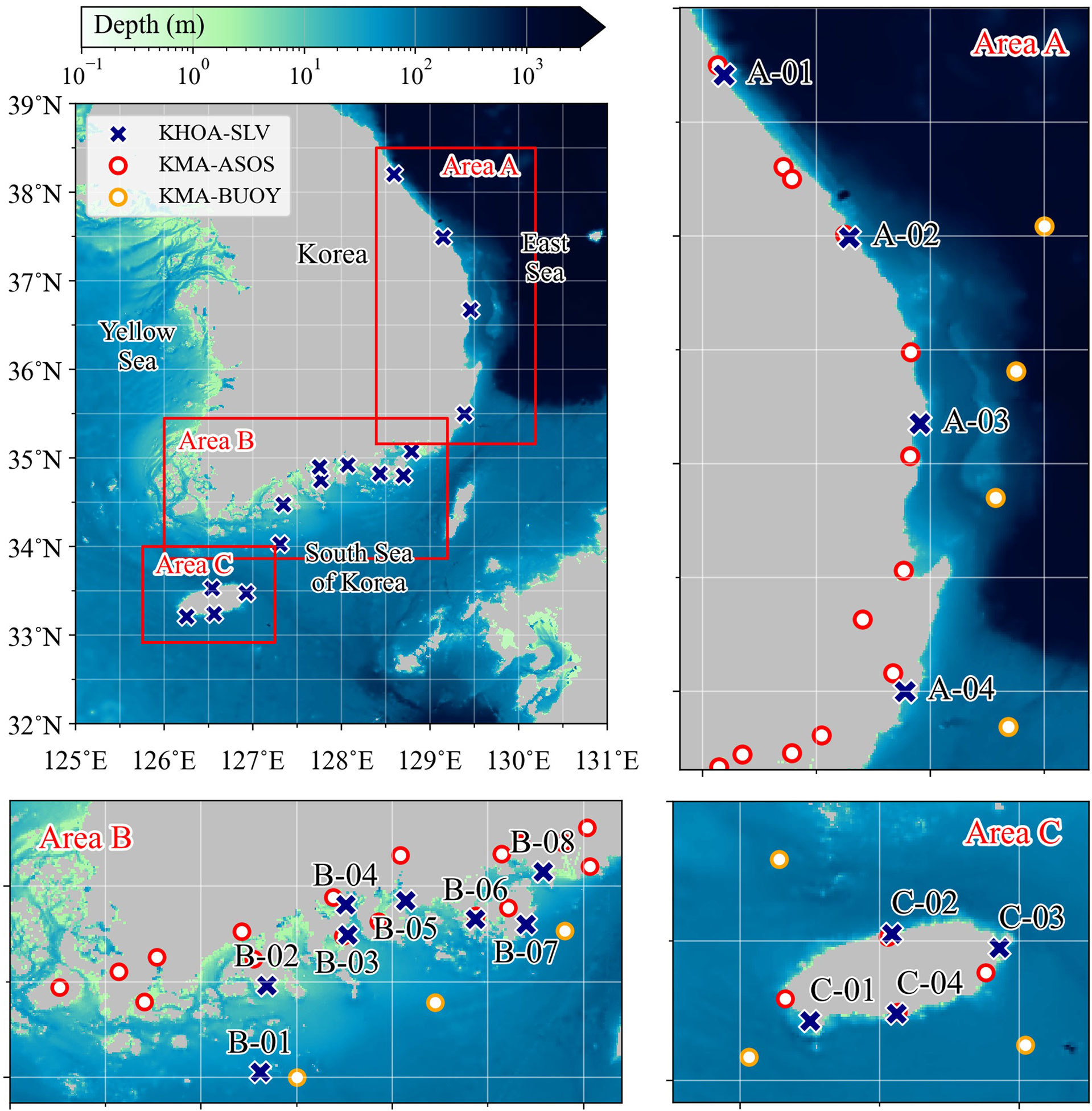
Figure 1 Study area and observatory locations. Navy crosses indicate the 16 tidal gauges at which the developed artificial neural network model will be applied. Red and orange circles indicate the ASOS stations located on the land and the ocean buoy, respectively.

TABLE 1

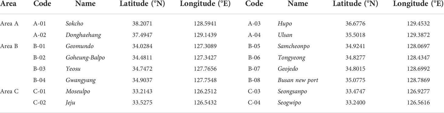
Table 1 Details of the 16 tidal gauges.

The 1-min sea-level data collected by the KHOA were preprocessed using the following methods. To leave only residual components, astronomical tides were removed from the sea-level data using the TIRA tidal analysis program in the TASK-2000 package (Murray, 1964; Bell et al., 1999). After simple quality control using the 3-sigma rule for the residual and the amount of change in the residual, a 3-h low-pass filter was applied to remove high-frequency noise remaining in the data. Thereafter, the data averaged for 1 h were linearly interpolated to fill in missing values of less than or equal to 3 h. This data processing, which is based on the confirmation of the signal-to-noise ratio, makes the model more robust. All the weather data of 30-min intervals were also 3-h low pass filtered and linearly interpolated for missing values of less than or equal to 3 h. The 30-min interval data were subsampled at hourly intervals corresponding to the processed sea-level data.

The residual (R) of the sea level from tides was the reconstruction target in this study, and the target of the ANN model was the amount of change in the residual (dR) over a unit time (1 h). This is because harmonic synthesis can reconstruct regular tidal fluctuations with high accuracy, and the ANN model can be prohibited from merely imitating rather than predicting the sea level values. In other words, if the input variable has target-like variability, the model will easily finish learning by giving this input a large weight (e.g., the sea level in the last hour or before one tide cycle). To avoid this situation, an autocorrelation analysis was performed on the observed sea level, R, and dR, and dR was selected as the ANN model target because its autocorrelation function converges most rapidly to zero over time.

Dataset

Instead of using all the collected data, the dataset for the ANN model should be chosen for efficient training and running. This is because the model used observational data, including missing data. These data gaps in the time series prevent the ANN from proper learning, such as their impact on traditional time-series analysis methods. To provide a basis for constructing the dataset, cross-correlation between the input and target was performed for each target point. Similar to the mechanism of numerical ocean models, solved using a finite difference method, actual oceanic features respond to forcing gradients. Hence, unlike most oceanographic studies that apply ANN that uses input variables directly, the gradients of forcing that cause sea-level fluctuations should also be adopted for inputs. Therefore, the inputs for correlation analysis include not only weather data (X) and their moving averages (rX), but also the gradient of weather data (dX) and the moving average of their gradient (rdX). The window for calculating the moving average was set to 5 h. In general, rdX, dX, rX and X are highly correlated with the target data. For the correlation analysis with the sea-level residual from 16 tidal gauges, a total of 258 weather variables were used, consisting of 8 categories collected from 43 observatories. The cross-correlation results are not shown due to the large number of results. During the process of preprocessing the input variables, the consideration of the various forcings applied to the target variable is important because it helps design a better performance model. Based on the analysis results, the input dataset for each target station consisted of data that were highly correlated with each weather element. In addition, R, and astronomical components and their envelopes that imply spring and neap tides were appended to the processing variables, and the sinusoidal and cosinusoidal of the date¹ were also added.

Unlike general ANN techniques, the test dataset is not used in this model set, since because the goal of this study is to reconstruct long-term gaps, and hence our model is trained to predict the sea-level change in just one step. Instead, it is reasonable to reconstruct the n- hour pseudo-gaps using a pre-learned weight set and then verify this time series. The additional ensemble dataset configurations and test methods are described below.

Training model and ensemble design

The ANN model was trained to output the sea-level change dR at the next time step by inputting oceanic and atmospheric data, and all constructed data had time-series properties. This study uses LSTM among the recurrent neural network (RNN) series, which is a method to solve the vanishing gradient problem of standard RNN. The ANN model in this study consisted of six layers, including one LSTM layer (Figure 2) and hyperparameters (Table 2). The feature has a funnel shape that continuously converges after expanding once past the input layer. Different for each target observatory, the features of the input were approximately 100. The nodes, which are scaled down after expanding in the first fully connected (FC) layer, compress the extracted features. To prevent overfitting, an early stop was used, and simultaneously to ensure certain learning progress, the minimum epoch was set to 500.

FIGURE 2

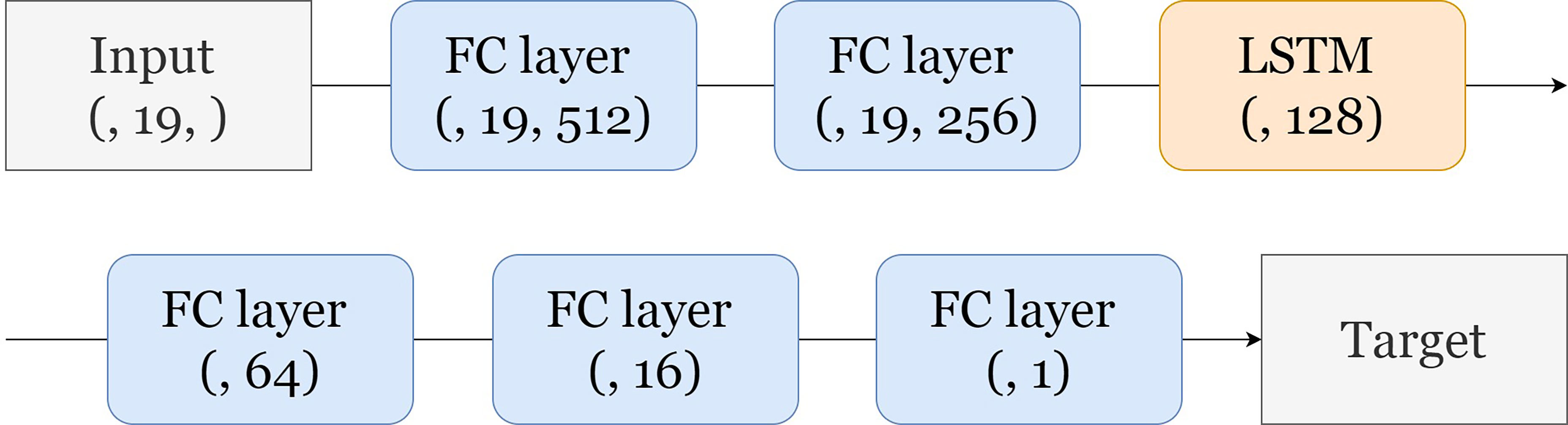
Figure 2 Structure of ANN model. FC denotes fully connected.

TABLE 2

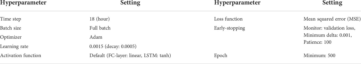
Table 2 Summary of model hyperparameters and their settings.

In machine learning, the ensemble of models makes the model performance more robust (Opitz and Maclin, 1999), which has been demonstrated in its application to LSTM (Guan and Plötz, 2017). In this study, a bagging ensemble was implemented to generalize the model as follows: The k-fold technique, with k=5, was used as the base. After dividing the date (1–31) of the data by 5, the remainder (0–4) is converted into an index. Five ensemble members were used as the validation set by matching each index. In this process, the data in each ensemble member were divided into an approximately 80% training set and an approximately 20% validation set. Five independent models were trained twice with a random initial state, and as a result, 10 ensemble members were established. The 10 models that were trained were ensemble-averaged for all possible combinations ($1023={\displaystyle \sum _{i=1}^{10}10}{C}_i$), and the combination with the smallest error during the 72-h data reconstruction was selected as the final ensemble model (EM) set.

Reconstruction of long-term missing values and data assimilation

The procedure for reconstructing the long-term sea-level gaps is as follows (Figure 3). When the input data set  (R_T−1, R^′_T−1, X_T) passes through the model weight set (W) that has been trained, the residual difference from the next time (R^′_t ) is

$\begin{array}{ll}{R^{\prime }}_t=W\left(R_{T-1}, {R^{\prime }}_{T-1}, X_T\right),& (1)\end{array}$

FIGURE 3

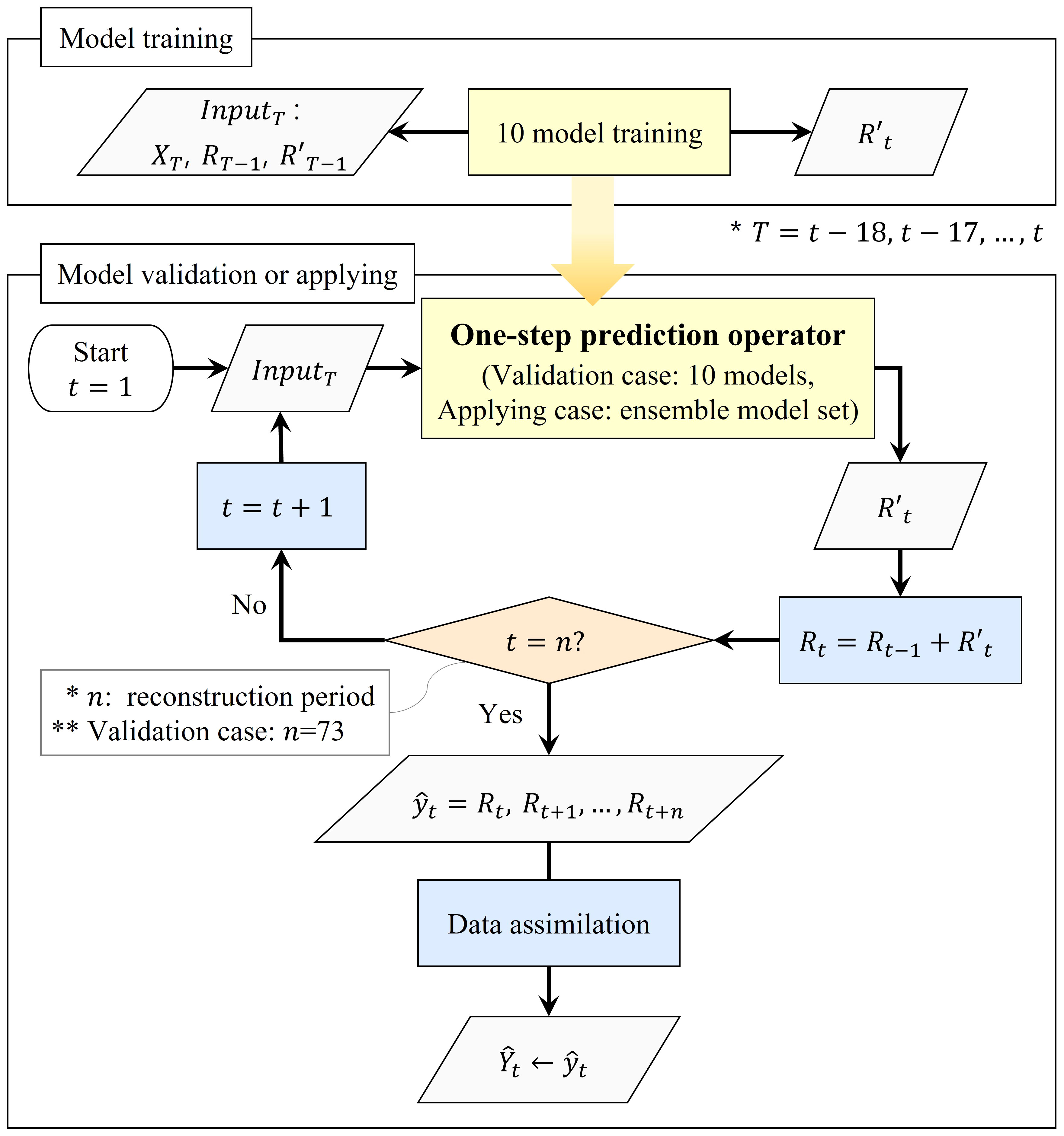
Figure 3 Flowchart of reconstruction for long-term sea-level gaps.

where t=1, 2, 3, … , n , and T :{t−18, t−17, …, t−1, t}. Therefore, the weight set acts as an operator for the one-step prediction. Because this operator can be used recursively, it can respond to long-term missing data using

$\begin{array}{ll}{R}_t=R_{t-1}+{R^{\prime }}_t& (2)\end{array}$

Theoretically, if there are no missing data in all inputs (X) except the reconstruction target, the model set can work indefinitely. In the technique using a general ANN, the interpolation target time is limited because of the constraint in which the shape of the target is fixed. However, the proposed method can be a powerful solution for the long-term gaps. Because the reconstruction of the missing values is performed based on the prediction, an unavoidable difference occurs between the predicted value at the end of the reconstruction and the observed value at that point. For a reconstructed value to substitute the observed value, it must be completely connected to the isolated observation. Therefore, we used a data assimilation technique to eliminate this difference. The assimilated data ${\widehat{Y}}_t$ can be expressed as follows:

$\begin{array}{ll}{\widehat{Y}}_t={\widehat{y}}_t-w_t{e}_t\left(\frac{{\widehat{y}}_n-y_n}{e_n}\right), & (3)\end{array}$

where t=1, 2, 3, …, n,  n is the continuous missing time+1, ${\widehat{y}}_t$is the reconstructed residual time series up to n-times, e_t is the statistical error time series (look-up table from the RMSE time series of each observatory), w_t is the time series of the data assimilation weight, ${\widehat{y}}_n$, y_n are residual predictions and observations at time n, and e_n is the statistical error value at time n. The w_t is a linear function from 0 to 1 divided by n. Expanding this formula has the following meanings. $\left({\widehat{y}}_n-y_n\right)/e_n$ refers to the ratio between the global averaged error and the rebuilt value error at the n-time step. Thus, $e_t\left({\widehat{y}}_n-y_n\right)/e_n$ are the values of applied the former ratio to the global averaged RMSE time series, and the sign is determined by the error at the endpoint of reconstruction. This term has a weakness that the use of mean RMSE time series implies the assumption of the monotone error increases (or decreases). Due to this precondition, if the error sign is switched as the reconstruction elapsed, the data assimilation performance in the first half of the prediction can be damaged. To compensate for this flaw, the w_t function is applied, which implies that we fully trust the predicted value at the start time of the reconstruction and the observed value at the end. Intuitive examples of data assimilation techniques are presented in Section 4.

We confirmed that more than 95% of the long-term gaps in the reconstructed sea-level data were continuous within 72 h, and the 72-h reconstruction model was verified using the above method. The theoretical number of time points for 72-h reconstruction is 43,848 (5 years ˟ days of year ˟ 24 h), and the practical number of points due to missing data is approximately 10,000 to 25,000 (different for each target). The ANN model performance was verified using the root-mean-squared error (RMSE) and the coefficient of determination (r²), defined as follows:

$RMSE= \sqrt{ \frac{1}{n} {\sum }^{}{\left(y_i-{\widehat{y}}_i\right)}^2}$, and

$\begin{array}{ll}{r}^2= \frac{{\sum }^{}{\left({\widehat{y}}_i-{\overline{y}}_i\right)}^2}{{\sum }^{}{\left(y_i-{\overline{y}}_i\right)}^2}& (4)\end{array}$

The RMSE time-series is used as a time function as a look-up table for data assimilation.

In summary, the method for the complete reconstruction of the sea level involves four procedures. First, ten independent models were trained and validated to predict R^′_t (or dR). Second, reconstruction of sea level was performed for 73 h using the learned weights that act as one-step prediction operator. At this time, 10 model sets including the operating process are used as ensemble members. Third, the test for the 1023 combinations of the ensemble average, of which the combination with the minimum error is selected as the EM. Finally, data assimilation was performed for the EM to produce a smoothly connected time series at the end point of the reconstruction (Figure 3).

Reconstruction model using fixed shape ANN and harmonic synthesis

In the previous study for gap-filling using ANN, it is common that the shape of output is fixed. Therefore, output shape should be same to missing periods for the reconstruction of long-term gaps (Contractor and Roughan, 2021; Ren et al., 2022). In other words, the number of models must be trained for corresponding to long-term missing periods. Additionally, the longer the reconstruction period, the lower the model performance. Our model set has been compared to a typical fixed shape ANN (F-ANN) model for performance assurance, and the validation time for the F-ANN is same as our model set, 72h. In addition, harmonic synthesis method is a sufficient tool to reconstruct the regular tidal sea level. Therefore, we assumed a situation that tidal sea level is rebuilt using the harmonic synthesis, which is the same as that the sea-level residual is predicted to be zero for every time. The harmonic synthesis was also performed for 72-h pseudo missing.

Results

Model validation

A combination of ten independent ANN models was evaluated for each tidal gauge station, and the ensemble mean with the lowest error was selected. At least five ensemble members were used in the combination, and some observatories used all the members. Figure 4 shows examples of the EM and data assimilated model (DAM) results for the reconstruction of 72-h sea-level gaps. They were selected for weather events caused by pressure jumps and typhoons with large sea level changes during 2016–2020.

FIGURE 4

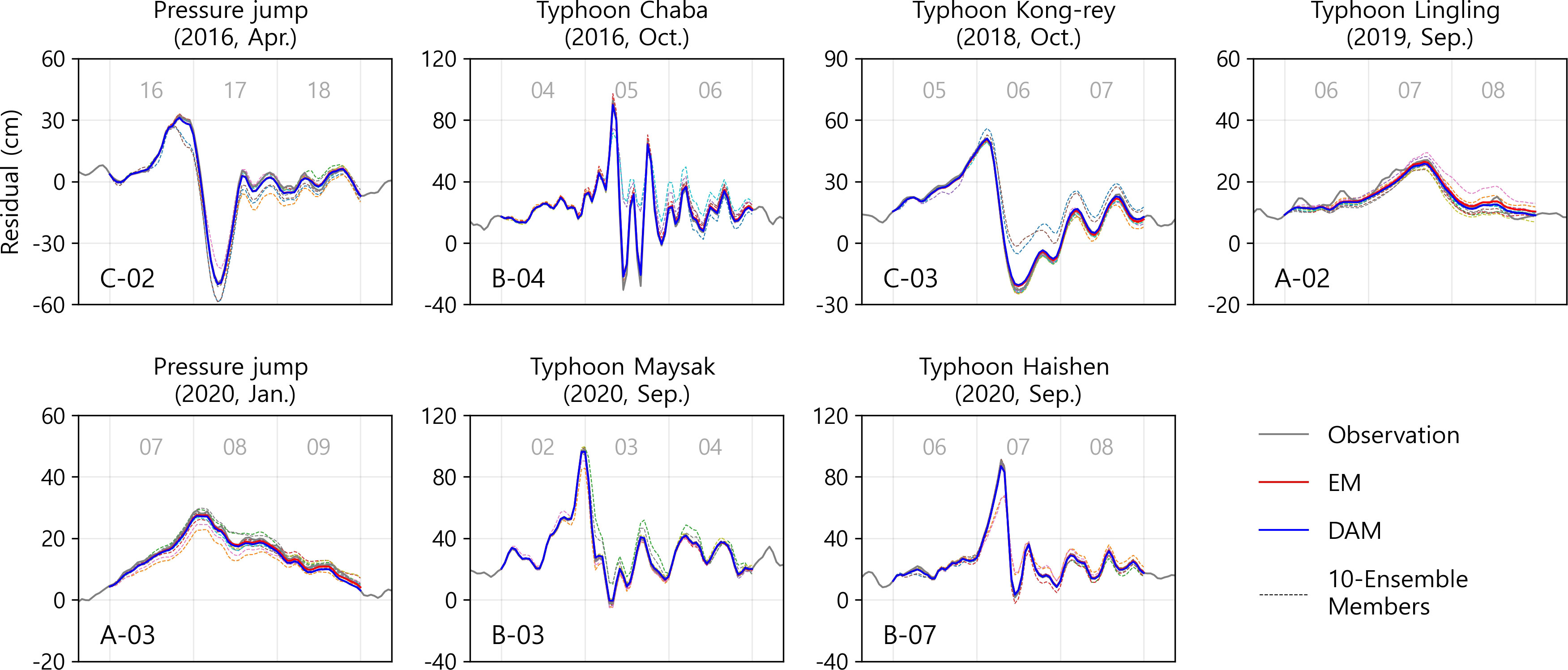
Figure 4 Examples of 72-h model reconstruction during weather events (pressure jumps and typhoons) during 2016–2020. The name of the station is written in the lower left corner of each sub-plots. Gray lines indicate observed sea levels. Red and blue lines represent predicted sea levels from EM and DAM, respectively. Dotted lines with different colors represent predicted sea levels from ten independent ensemble members.

The results of an EM (red solid line) comprising an optimal combination of ensemble members (dotted lines) with high variance are shown. Several ensemble members tend to underestimate or overestimate the sea level, and these members are excluded from the final ensemble member combining process. The EM selected from 10 independent models performed better than the model using a single dataset. In addition, although the prediction of the EM presented sufficiently acceptable gap-filling results, the application of the data assimilation technique improved the model results by producing a seamless continuity between the predicted and observed values at the end point of the gap. Notable impacts caused by data assimilation are observed at A-02 and A-03, where the predicted sea level values from the EM shift 1.1 of 1.2 cm, respectively.

The performance of the reconstruction was validated for the prediction operator (EM) and the DAM separately. Figure 5 shows the validation results of the reconstructed values, assuming a maximum of 72 h of data gap. Although there were some deviations for each tidal gauge, the validation results showed the same pattern for each target gauge. Both the EM (black line) and DAM (yellow line) results show that the average RMSE (solid line) increased and the r² (dotted line) decreased as it responded to long-term missing data. This is because the missing residuals are reconstructed using the forward prediction method; thus, the longer the prediction period, the greater the error expansion. Data assimilation was applied to eliminate this expanded error, which reduced not only the error at the end of the reconstruction, but also within the reconstruction period. Hence, a better 72-h reconstruction performance was obtained when data assimilation was applied.

FIGURE 5

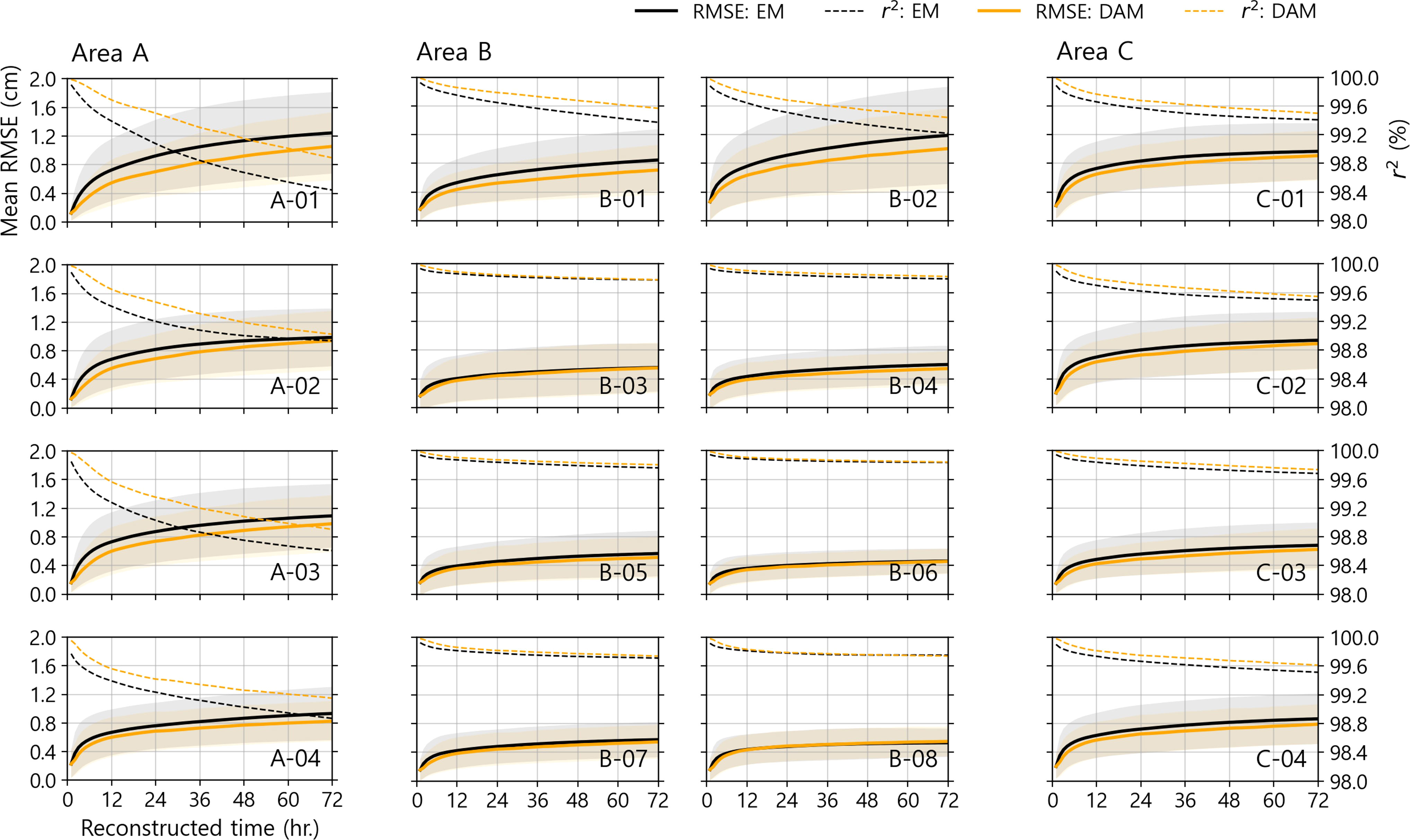
Figure 5 72-h reconstruction validation time series. RMSE and r² are represented by solid and dotted lines, respectively. Additionally, the EM and DAM results are shown in black and orange, respectively. The shading area denotes one standard deviation of the data for the mean RMSE validation of each time.

For convenience, the research areas were grouped into areas A, B, and C, based on their topographic characteristics. The time series of RMSE (or r²) showed similar patterns for each area. First, the tidal gauges in Area A were further from each other than in the other areas, and their distribution was meridional along the coastline. Because of the geographical features, the tidal gauges in Area A experienced data deficiency for close distance observatories, thus performing the worst of the three areas. However, because the tidal gauges and observatories in Area B are relatively dense, the oceanic and atmospheric data are fully dependent on the training process. Therefore, Area B performed the best on average among the three areas. While the models performed well, stations B-03 to B-07 did not seem to have outstanding data assimilation performance, and even in B-08, the DAM results were worse than those of the EM. However, in terms of considering the variability of the residual values and the EM error, this defect is acceptable. The RMSE of these stations was up to 0.6 cm, which is much less than the average standard deviation of the residual values for these stations, 13.1 cm. In addition, because the time series of relatively small errors appears as random walking (white noise), these stations do not fully benefit from data assimilation techniques, which provide the maximum advantage for monotone increases (or decreases) in errors. The B-01 and B-02 stations, unlike the above neighboring stations, show time series of errors that reveal increasing (or decreasing) trends. Therefore, these stations have relatively large errors and are thus highly efficient in terms of DA. The tidal gauges in Area C were located on an island off the coast. In this area, residual fluctuations appear to be between Areas A and B, as do the tendencies of the model’s performance.

On the 72-h reconstruction for sea-level data gaps, the minimum RMSE is 0.5 cm for both the EM and the DAM at B-06, and the maximum RMSE is 1.3 and 1.1 cm for the EM and the DAM at A-01, respectively (Table 3). These results imply that the 72-h reconstruction ANN model developed in this study guarantees an error of 1.1 cm or less. In case of comparison with data variability (standard deviation; STD.), normalized RMSE is calculated, in which EM and DAM are less than 10%. As mentioned above, station A-01 shows the worst performance because close distance weather data are rare, and tidal gauges are unavailable to the north, unlike other tidal gauge sites. The importance of the data obtained from nearby weather stations and tidal gauges can also be confirmed by the average error of each area. Area B, which can refer to dense data, has the lowest mean error and in Area A, and vice versa.

TABLE 3

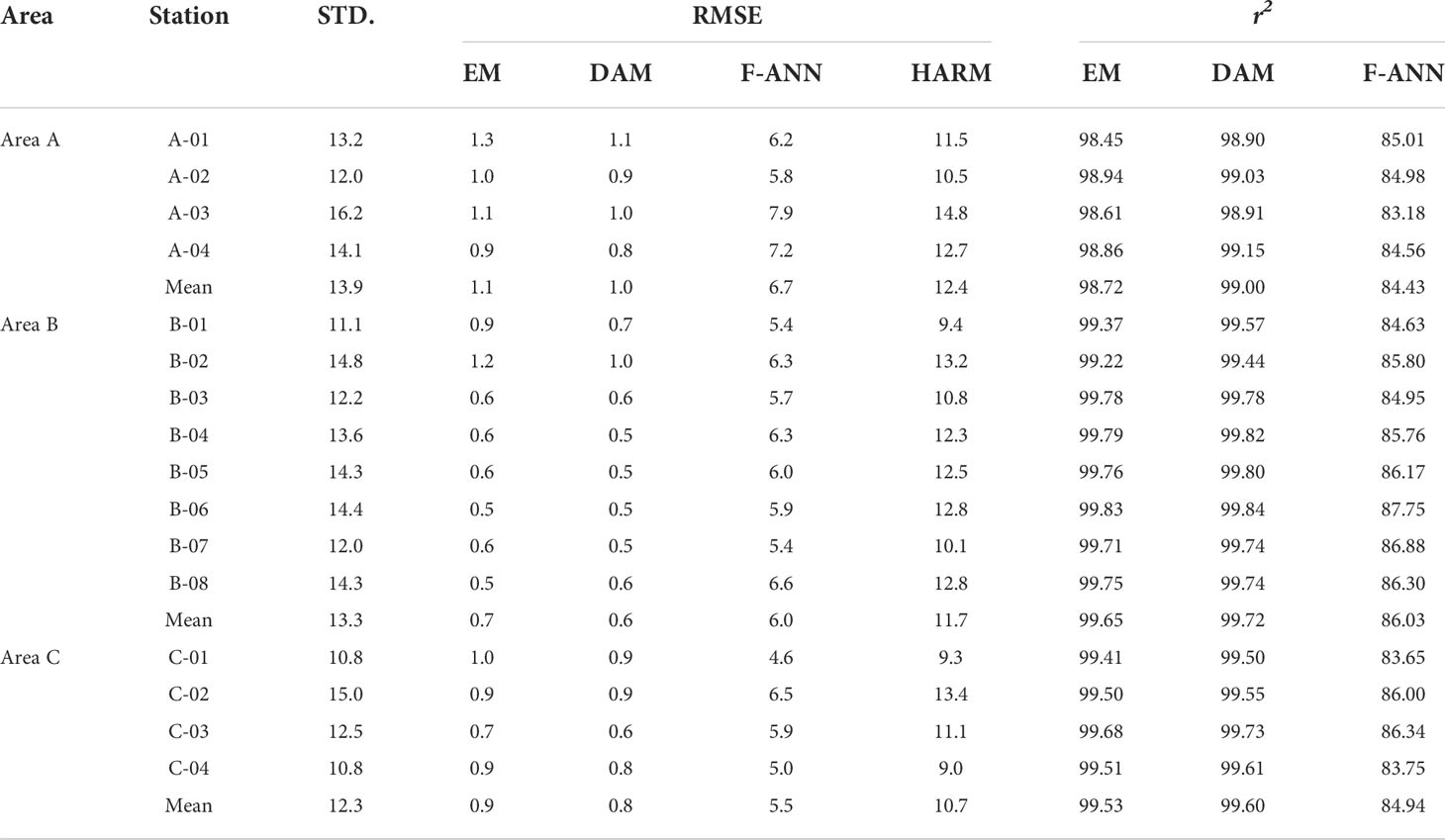
Table 3 Performance of ensemble model and data assimilation model at 16 tidal gauge stations. (Unit of standard deviation and RMSE: cm).

RMSEs of the F-ANN are calculated as 4.6 to 7.9cm, and the range of NRMSE is 41.3 to 50.8%. This result, which is worse than EM and DAM, is considered to be due to the number of output features being 72 for F-ANN, while 1 for the one-step prediction operator. ANN model is trained by reducing the mean error of the overall dataset. Thus, the weights of 72 nods cannot be specialized, so that, a generalized (standardized) model could be trained. Next, reconstruction of the sea-level missing by the harmonic synthesis is only predicting regular tidal components, and is the same as ignoring the sea-level residuals. The RMSEs of these predictions are calculated as 9.0 to 14.8cm, which is a similar level to the variabilities of the sea-level residual.

Application to missing data

Models that have been validated from reconstruction by a one-step operator for data assimilation can be applied to fill real sea-level data gaps. In addition, by redeeming the reconstructed value with the true value, the iterative reconstruction of other observatories is possible. In other words, it is possible to activate the time zones that have been deactivated owing to missing input data (sea level at other stations) through repeated reconstruction. The reconstruction was repeated seven times and the results are presented in Table 4. The position with the highest reconstructability was A-01, where 93.6% of the gaps were successfully reconstructed. Conversely, C-03 station shows the lowest reconstructability, with 39% (733 times) of the sea-level gaps being continuous at the end of the study period.

TABLE 4

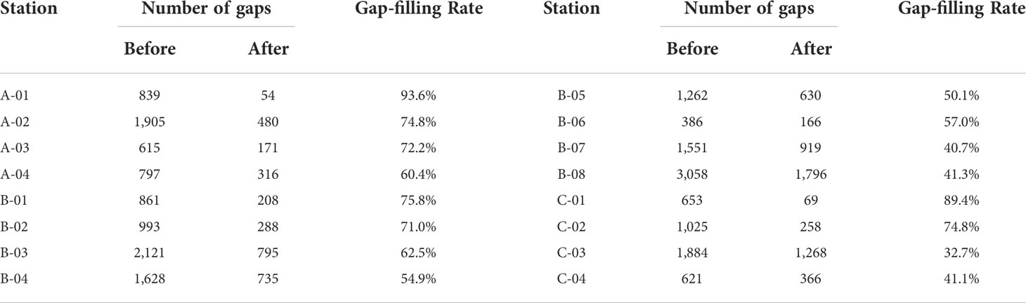
Table 4 Data gap-filling rates at 16 tidal gauge observatories by the ANN model.

Among the reconstruction results from the actual gaps, an example of the longest period for each station is presented in Figure 6. The longest reconstruction period was 290 h at B-01 station. Despite the long-term reconstruction of more than 12 days, the difference between the observed and predicted values at the end of gap filling was less than 1 cm. B-03 station shows another notable result. The sea-level values for the 62-h data gap were reconstructed in the 3rd iteration interpolation. The prediction-observation difference at the endpoint converges, implying that reconstruction by repetition can yield reasonable results. In terms of the time variability of the reconstructed residuals, Area A shows that the variabilities are less than those in the other areas. Of all the areas, the meteorological tide constituted most of the residual fluctuation because the least tidal energy came into Area A. In contrast, in Area B, which has a complex coastal topography, nonlinear tidal components could not be removed in the harmonic analysis process. Consequently, the remaining components cause large residual fluctuations in this area. The component properties and variability of Area C were between those of Areas A and B.

FIGURE 6

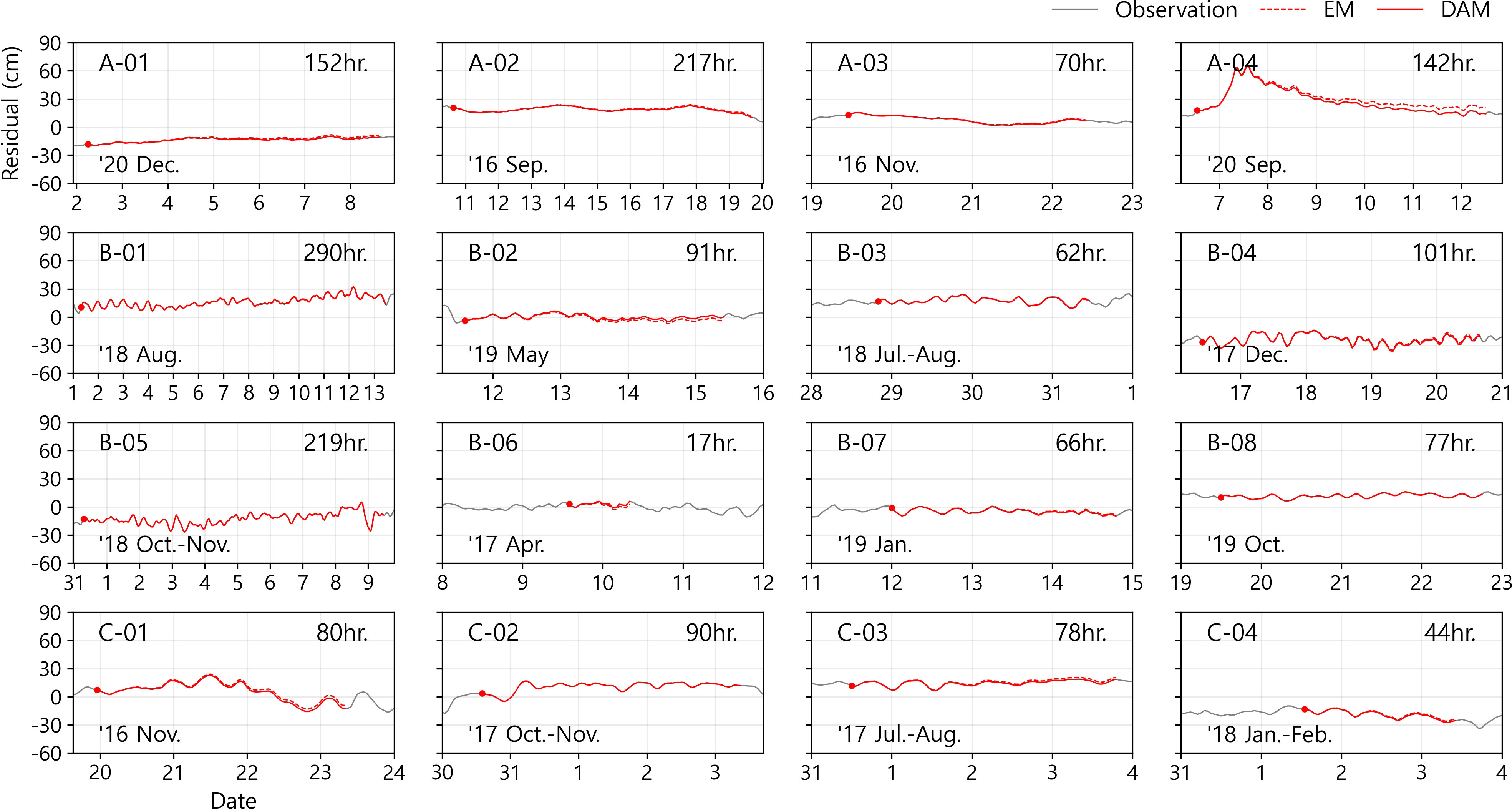
Figure 6 Examples of longest reconstruction of real sea-level data gaps at each tidal gauge station. Cases are excluded when data assimilation cannot be applied due to the absence of observations at the predicted end point. The gray solid lines represent the observation values, and the red dotted lines show the EM results produced by using the one-step operator. The red lines indicate that the reconstructed value is adjusted to match the observed value using data assimilation.

In terms of the reconstructability, these differences between the values tend to be independent for each station rather than being similar by sea area. The reason and improvement possibility for this flaw can be considered in two main parts. Above all, missing of input data should be minimized for successful reconstruction. Training input data include the sea-level residual of nearby tidal gauges as well as the weather data. And hence, if the weather event (or disaster) occurs, reconstruction is hindered due to the simultaneous missing of the sea-level values at the adjacent stations. While we considered mutual missing time in the inputs for curtailing negative effects, that treatment could not be the complete solution. One way to alleviate this problem is to compose several input sets, which have missing time that do not overlap with each other. As the result, the model set can be expected to get a higher reconstructability, although the errors may be increased due to the removal of major features. The second to be considered factor is that endpoint observation values for data assimilation are essential.

As a practical example, predictive interpolation was performed at stations B-03 and B-04 over a longer period, as shown in Figure 6 (152 and 157 h, respectively). However, there were no observations to be used for data assimilation at the end points, which hindered complete gap filling. And it is the same that the reason for the lowest gap-filling rate at the station C-03. The sea-level data collected this station contains continuous gaps for 730 h, which are located at the observed end time and account for 39% of all the missing times. Even if EM can be performed, the reconstruction is not completed because data assimilation cannot be operated. To solve the part of this problem, we can make a suggestion to combine methods of backward predictions with our forward predictions, but it also would not be a complete solution.

Discussion

A data assimilation example at A-01 station shows all the needs, advantages, and weaknesses of the data assimilation (Figure 7). First, regardless of whether a linear weight function (w_t) is used, the predicted endpoint value must be continuous with the observation value at that point to serve as a substitute for the observation data (without weights means w_t=1; constant function). The June example demonstrates the advantages of data assimilation using linear weights. When the linear weights were used (standard DAM), the RMSE reduced to 0.7 cm from 2.4 and 2.2 cm, which are RMSE values for the EM and the DAM without weights, respectively. Conversely, the December example shows the weakness of the DA. This technique has the precondition implied in Equation (4), in which the error increases only in one direction. Therefore, when the sign of the model error is swapped, the damage caused by data assimilation occurs in the first half of the interpolation and the gain occurs in the second half. In the case of the predicted model and data assimilated with/without linear weights, RMSEs were calculated to be 2.3, 1.5, and 2.1 cm, respectively. Despite some losses, it is evident that the process of matching end-to-end data is essential. Hence, data assimilation using linear weights is indispensable. From these two examples, we can confirm that the propagated prediction error and additional error due to data assimilation in this example are mitigated using linear weights.

FIGURE 7

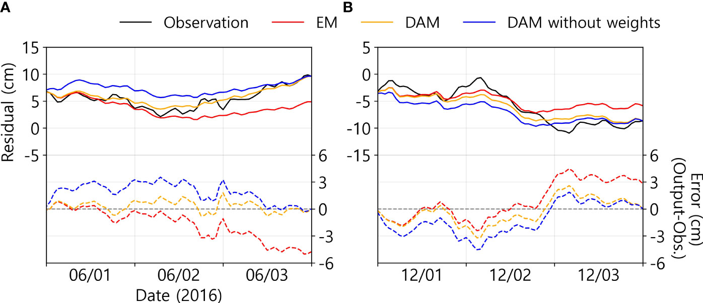
Figure 7 Examples of validation time series at A-01 station. (A) optimal data assimilation case (B) case of supplement for the weakness of data assimilation by using linear weights. The black solid line represents the observation data. Red, orange, and blue colors indicate the EM predicted values, DAM predicted values using linear weights, and not using, respectively. The solid lines denote the residual values, and the dashed lines denote the difference between the reconstructed residuals and the observations.

The target of this study is the sea-level residual (R) excluding regular tidal elevation, which implies that weather input data should be the essential element for the success of the ANN model’s sea-level prediction. However, when coastal seas are affected by severe weather events, the ANN operator tends to be deactivated because of an increase in missing data. During the data sorting described in Section 2.2, we considered not only the correlation between the data but also the missing rate. Nonetheless, the existence of missing values in input data is inevitable. Therefore, we executed a sensitivity test with and without weather data, and examined the reconstructability and accuracy to evaluate the performance of the reconstruction model (Figure 8). Case 0 is the original model set, including weather data, and Case1 is the model set excluding all weather data.

FIGURE 8

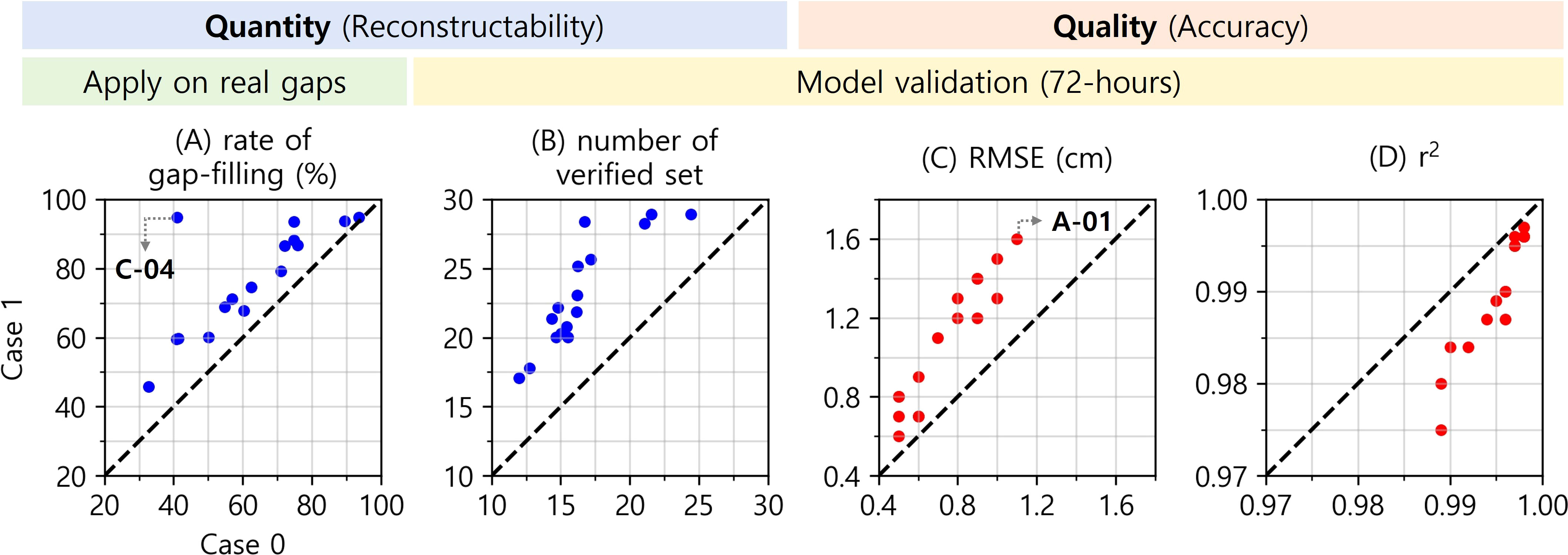
Figure 8 Comparison of reconstructability and accuracy in two cases with (Case 0) and without (Case 1) the atmospheric data for the ANN model input. (A, B) Reconstructability on real gaps and 72-h model validation. (C, D) RMSE and r² on model validation. X- and Y-axes in all four scatter plots represent Case 0 and Case 1, respectively.

The reconstruction rate of Case 1 shows an increase at all stations compared to Case 0 (Figure 8A). Most importantly, the gap-filling rate at C-04 increased by 53.8%p (from 41.1% to 94.9%), as almost all the deficiencies were filled. This indicates that the operator was more efficient in removing missing data from weather data. In addition, it was confirmed that the substitutes, reconstructed sea-level values, were used as inputs for additional gap filling at nearby tidal gauge stations. In other words, successful reconstruction at close distance tidal gauges propagates a favorable function during the iterative gap-filling procedure. The number of 72-h consecutive reconstruction datasets for model verification also increased in Case 1 (Figure 8B). Contrary to the previous positive effect, the reconstruction accuracy was lower in Case 1 than in Case 0 (Figures 8C, D). RMSE increased up to 0.5 cm, and r² value decreased to 0.014. These results were obtained by ignoring the local weather effect when reconstructing the sea-level residual. In particular, A-01 tidal gauge station, where the performance of sea-level reconstruction was the worst, had the least ASOS weather stations and nearby tidal gauges.

The reconstruction model that excluded weather features showed positive and negative effects in terms of quantity and quality, respectively. Because both are parts that cannot be disregarded in research performance, a reasonable balance is necessary. As mentioned above, we could not completely rule out the missing data included in the weather data, despite our efforts to balance this. Therefore, if this study is to be applied to practical situations, it is essential to merge multiple models using datasets designed from various perspectives. In other words, for complete reconstruction, the top priority is to avoid overlapping missing periods between the datasets.

Conclusion

In this study, a reconstruction tool was developed to ensure the continuity of sea-level time series using ANN techniques. The target is the sea-level residual, which excludes regular astronomical tides from sea-level observations, and the input data are the residuals and weather elements from nearby stations. The trained weight set was designed to respond flexibly to long-term missing data by acting as a one-step prediction operator. This is a good example of overcoming the limitations of the existing ANN techniques that require a fixed output shape. The forward predicted residuals should be connected to the observations at the reconstruction end point such that it can be truly meaningful as a gap-filled value. Therefore, we developed and applied a data assimilation technique to predict values based on the reliability between the observations and predicted values. As a result, the ANN model was confirmed to successfully reconstruct the residuals with an RMSE between 0.5 and 1.1 cm for the 72-h average accuracy at 16 tidal gauge observatories. Finally, the validated DAM was also applied to actual missing data situations. The longest gap-filling period was 290 h, and the maximum rate of gap-filling was 93.6%.

The strengths and weaknesses of DA, which is an essential process for a successful ANN model, were analyzed. Additionally, the contribution of the linear weights used to relieve defects in data assimilation was examined. Finally, model sensitivity was analyzed for the presence or absence of weather features in the input data. As a result, it was confirmed that more weather factors could improve the qualitative performance of the model, but could decrease the quantitative performance owing to the missing values in sea-level records. Consequently, to obtain the best qualitative and quantitative performance, we conclude that an appropriate balance is necessary when weather features are added to the ANN model.

To deal with missing sea-level values, we used an ANN that can deal with nonlinearity, multiple variables, and multiple times. Owing to the influence of local topography, sea-level values show spatiotemporal variability. Nonetheless, based on our flexible data processing and technique design, we achieved satisfactory results at all observatories despite using the same single model structure. Therefore, this technique can be sufficiently applied not only to sea-level records, as in this study, but also to fill in the frequent data gaps in various oceanic and atmospheric observations.

Data availability statement

The datasets presented in this study can be found in online repositories. The names of the repository/repositories and accession number(s) can be found below: Sea-level records are available at http://www.khoa.go.kr/oceangrid/gis/category/reference/distribution.do. The ASOS data are available at https://data.kma.go.kr/data/grnd/selectAsosRltmList.do?pgmNo=36. Buoy data were obtained from https://data.kma.go.kr/data/sea/selectBuoyRltmList.do?pgmNo=52.

Author contributions

E-JL: Primary writing and calculation. KK: Data collection and discussion. J-HP: Overall coordination and discussion. All authors contributed to the article and approved the submitted version.

Funding

This work was supported by “Development of 3-D Ocean Current Observation Technology for Efficient Response to Maritime Distress” funded by Korea Institute of Marine Science & Technology Promotion (20210642).

Conflict of interest

The authors declare that the research was conducted in the absence of any commercial or financial relationships that could be construed as a potential conflict of interest.

Publisher’s note

All claims expressed in this article are solely those of the authors and do not necessarily represent those of their affiliated organizations, or those of the publisher, the editors and the reviewers. Any product that may be evaluated in this article, or claim that may be made by its manufacturer, is not guaranteed or endorsed by the publisher.

Footnotes

1. ^ sin (day-of-year / days of the year ˟ 2 ˟ pi), cos (day-of-year / days of the year ˟ 2 ˟ pi)

References

Adytia D., Saepudin D., Pudjaprasetya S. R., Husrin S., Sopaheluwakan A. (2022). A deep learning approach for wave forecasting based on a spatially correlated wind feature, with a case study in the Java Sea, Indonesia. Fluids 7(1), 39. doi: 10.3390/fluids7010039

CrossRef Full Text | Google Scholar

Bell C., Vassie J. M., Woodworth P. L. (1999). POL/PSMSL tidal analysis software kit 2000 (TASK-2000). 2000UKCCMS proudman oceanographic laboratory permanent service for mean Sea level.

Google Scholar

Bosch W., Dettmering D., Schwatke C. (2014). Multi-mission cross-calibration of satellite altimeters: Constructing a long-term data record for global and regional Sea level change studies. Remote Sens. 6, 2255–2281. doi: 10.3390/rs6032255

CrossRef Full Text | Google Scholar

Cane M. A., Kaplan A., Miller R. N., Tang B., Hackert E. C., Busalacchi A. J. (1996). Mapping tropical pacific sea level: Data assimilation via a reduced state space kalman filter. J. Geophys. Res. Oceans 101, 22599–22617. doi: 10.1029/96jc01684

CrossRef Full Text | Google Scholar

Carton J. A. (2005). Sea Level rise and the warming of the oceans in the simple ocean data assimilation (SODA) ocean reanalysis. J. Geophys. Res. 110, C09006. doi: 10.1029/2004jc002817

CrossRef Full Text | Google Scholar

Cheon S.-H., Hamlington B. D., Suh K.-D. (2018). Reconstruction of sea level around the Korean peninsula using cyclostationary empirical orthogonal functions. Ocean Sci. 14, 959–970. doi: 10.5194/os-14-959-2018

CrossRef Full Text | Google Scholar

Contractor S., Roughan M. (2021). Efficacy of feedforward and LSTM neural networks at predicting and gap filling coastal ocean timeseries: Oxygen, nutrients, and temperature. Front. Mar. Sci. 8. doi: 10.3389/fmars.2021.637759

CrossRef Full Text | Google Scholar

Cooley S., Schoeman D., Bopp L., Boyd P., Donner S., Ghebrehiwet D. Y., et al. (2022). “Oceans and coastal ecosystems and their services,” in Climate change 2022: Impacts, adaptation and vulnerability. contribution of working group II to the sixth assessment report of the intergovernmental panel on climate change. Eds. Pörtner H.-O., Roberts D. C., Tignor M., Poloczanska E. S., Mintenbeck K., Alegría A., Craig M., Langsdorf S., Löschke S., Möller V., Okem A., Rama B. (Cambridge, UK and New York, USA: Cambridge University Press), 379–550. doi: 10.1017/9781009325844.005

CrossRef Full Text | Google Scholar

Dogan G., Ford M., James S. (2021). “Predicting ocean-wave conditions using buoy data supplied to a hybrid RNN-LSTM neural network and machine learning models,” in 2021 IEEE International Conference on Machine Learning and Applied Network Technologies (ICMLANT), pp. 1–6. doi: 10.1109/icmlant53170.2021.9690528

CrossRef Full Text | Google Scholar

Fourrier M., Coppola L., Claustre H., D’ortenzio F., Sauzède R., Gattuso J.-P. (2020). A regional neural network approach to estimate water-column nutrient concentrations and carbonate system variables in the Mediterranean Sea: CANYON-MED. Front. Mar. Sci. 7. doi: 10.3389/fmars.2020.00620

CrossRef Full Text | Google Scholar

Guan Y., Plötz T. (2017). Ensembles of deep LSTM learners for activity recognition using wearables. Proc. ACM Interactive Mobile Wearable Ubiquitous Technol. 1, 1–28. doi: 10.1145/3090076

CrossRef Full Text | Google Scholar

Hamlington B. D., Leben R. R., Strassburg M. W., Kim K. Y. (2014). Cyclostationary empirical orthogonal function sea-level reconstruction. Geosci. Data J. 1, 13–19. doi: 10.1002/gdj3.6

CrossRef Full Text | Google Scholar

Hochreiter S., Schmidhuber J. (1997). Long short-term memory. Neural Comput. 9, 1735–1780. doi: 10.1162/neco.1997.9.8.1735

PubMed Abstract | CrossRef Full Text | Google Scholar

Huang C. J., Kuo P. H. (2018). A deep CNN-LSTM model for particulate matter (PM2.5) forecasting in smart cities. Sensors 18 (7), 2220. doi: 10.3390/s18072220

CrossRef Full Text | Google Scholar

KHOA (2020). Ocean information (2020) (in Korean). Vol. 4 (Korea Hydrographic and Oceanographic Agency) 62–65.

Google Scholar

Kim K.-S., Lee J.-B., Roh M.-I., Han K.-M., Lee G.-H. (2020). Prediction of ocean weather based on denoising AutoEncoder and convolutional LSTM. J. Mar. Sci. Eng. 8, 805. doi: 10.3390/jmse8100805

CrossRef Full Text | Google Scholar

Lee E.-J., Chae J.-Y., Park J.-H. (2020). Reconstruction of Sea level data around the Korean coast using artificial neural network methods. J. Coast. Res. 95, 1172–1176. doi: 10.2112/si95-227.1

CrossRef Full Text | Google Scholar

Lu W., Su H., Yang X., Yan X.-H. (2019). Subsurface temperature estimation from remote sensing data using a clustering-neural network method. Remote Sens. Environ. 229, 213–222. doi: 10.1016/j.rse.2019.04.009

CrossRef Full Text | Google Scholar

Murray M. T. (1964). A general method for the analysis of hourly heights of tide. Int. Hydrographic Rev. 41 (2), 91–101.

Google Scholar

Nardelli B. B. (2020). A deep learning network to retrieve ocean hydrographic profiles from combined satellite and In situ measurements. Remote Sens. 12, 3151. doi: 10.3390/rs12193151

CrossRef Full Text | Google Scholar

Opitz D., Maclin R. (1999). Popular ensemble learning: An empirical study. J. Artif. Intell. Res. 11, 169–198. doi: 10.1613/jair.614

CrossRef Full Text | Google Scholar

Pappas C., Papalexiou S. M., Koutsoyiannis D. (2014). A quick gap filling of missing hydrometeorological data. J. Geophys. Res. Atmos. 119, 9290–9300. doi: 10.1002/2014jd021633

CrossRef Full Text | Google Scholar

Park J.-H., Watts D. R. (2005). Response of the southwestern Japan/East Sea to atmospheric pressure. Deep-Sea Res. II: Top. Stud. Oceanogr. 52, 1671–1683. doi: 10.1016/j.dsr2.2003.08.007

CrossRef Full Text | Google Scholar

Pugh D., Woodworth P. (2014). Sea-Level science: Understanding tides, surges, tsunamis and mean Sea-level changes Vol. 74 (Cambridge: Cambridge University Press), 262. doi: 10.1017/CBO9781139235778

CrossRef Full Text | Google Scholar

Ren H., Cromwell E., Kravitz B., Chen X. (2022). Technical note: Using long short-term memory models to fill data gaps in hydrological monitoring networks. Hydrol. Earth Syst. Sci. 26, 1727–1743. doi: 10.5194/hess-26-1727-2022

CrossRef Full Text | Google Scholar

Shao C., Zhang W., Sun C., Chai X., Wang Z. (2015). Statistical prediction of the south China Sea surface height anomaly. Adv. Meteorol. 2015, 1–9. doi: 10.1155/2015/907313

CrossRef Full Text | Google Scholar

Silva M. T., Gill E. W., Huang W. (2018). An improved estimation and gap-filling technique for Sea surface wind speeds using NARX neural networks. J. Atmos. Ocean. Technol. 35, 1521–1532. doi: 10.1175/jtech-d-18-0001.1

CrossRef Full Text | Google Scholar

Song T., Jiang J., Li W., Xu D. (2020). A deep learning method with merged LSTM neural networks for SSHA prediction. IEEE J. Sel. Top. Appl. Earth Obs. Remote Sens. 13, 2853–2860. doi: 10.1109/jstars.2020.2998461

CrossRef Full Text | Google Scholar

Turki I., Laignel B., Kakeh N., Chevalier L., Costa S. (2015). A new hybrid model for filling gaps and forecast in sea level: Application to the eastern English channel and the north Atlantic Sea (western France). Ocean Dyn. 65, 509–521. doi: 10.1007/s10236-015-0824-z

CrossRef Full Text | Google Scholar

Wenzel M., Schröter J. (2010). Reconstruction of regional mean sea level anomalies from tide gauges using neural networks. J. Geophys. Res. 115, C08013. doi: 10.1029/2009jc005630

CrossRef Full Text | Google Scholar

Zhang K., Geng X., Yan X.-H. (2020). Prediction of 3-d ocean temperature by multilayer convolutional LSTM. IEEE Geosci. Remote Sens. Lett. 17, 1303–1307. doi: 10.1109/lgrs.2019.2947170

CrossRef Full Text | Google Scholar