How artificial potential field algorithms can help to simulate trade-offs in movement behaviour of reef fishes

Kruse, Maren; Meyer, Christian; Schneekloth, Fabian; Reuter, Hauke

doi:10.3389/fmars.2022.1037358

ORIGINAL RESEARCH article

Front. Mar. Sci., 16 December 2022

Sec. Marine Ecosystem Ecology

Volume 9 - 2022 | https://doi.org/10.3389/fmars.2022.1037358

How artificial potential field algorithms can help to simulate trade-offs in movement behaviour of reef fishes

Maren Kruse^1,2*

Christian Meyer¹

Fabian Schneekloth^1,3

Hauke Reuter^1,2

¹Department Theoretical Ecology and Modelling, Leibniz Centre for Tropical Marine Research (ZMT), Bremen, Germany
²Faculty of Biology and Chemistry, University of Bremen, Bremen, Germany
³Faculty of Informatics, University of Bremen, Bremen, Germany

Introduction: Space use patterns in fish result from the interactions between individual movement behaviour and characteristics of the environment. Herbivorous parrotfishes, for instance, are constrained by the availability of resources and different predation risks. The resulting spatial distribution of the fish population can strongly influence community composition and ecosystem resilience.

Methods: In a novel approach, we combine individual-based modelling (IBM) with an artificial potential field algorithm to realistically represent fish movements and the decision-making process. Potential field algorithms, which are popular methods in mobile robot path planning, efficiently generate the best paths for an entity to navigate through vector fields of repellent and attracting forces. In our model the repellent and attracting forces are predation risk and food availability, both implemented as separate grid-based vector fields. The coupling of individual fish bioenergetics with a navigation capacity provides a mechanistic basis to analyse how the habitat structure influences population dynamics and space utilization.

Results: Model results indicate that movement patterns and the resulting spatial distributions strongly depend on habitat fragmentation with the bioenergetic capacity to spawn and reproduce being particularly susceptible processes at the individual level. The resulting spatial distributions of the population are more irregularly distributed among coral reef patches the more the coral reef habitat becomes fragmented and reduced.

Discussion: This heterogeneity can have strong implications for the delivered ecosystem functioning, e.g., by concentrating or diluting the grazing effort. Our results also highlight the importance of incorporating individual foraging-path patterns and the spatial exploitation of microhabitats into marine spatial planning by considering the effects of fragmentation. The integration of potential fields into IBMs represents a promising strategy to advance our understanding of complex decision-making in animals by implementing a more realistic and dynamic decision-making process, in which each fish weighs different rewards and risks of the environment. This information may help to identify core areas and essential habitat patches and assist in effective marine spatial management.

1. Introduction

Movement of organisms is a key issue in naturally fragmented landscapes (Turchin, 1991; Zollner et al., 1999) like tropical coastal habitats, and an important link between individual life history and population dynamics (Nathan et al., 2008; Morales et al., 2010; McClintock et al., 2014). Also, animal movement is one of the primary ways that mobile organisms can adapt to changing environments (Railsback et al., 1999; Smouse et al., 2010). This makes movement at all different spatial scales relevant to most current environmental concerns in the marine realm like coastal development, overexploitation of natural resources, or increasing degradation of habitats (Nathan et al., 2008).

Animal movement behaviour is notoriously complex and generally considered to consist of directed responses to social and environmental cues, resulting in space use patterns that represent trade-offs between energy gain, survival, and reproduction (Davis et al., 2017). Also, the possible involvement of many different environmental factors such as predation risk and habitat complexity as top-down controls or food availability as bottom-up drivers (Roff et al., 2019) complicate the analysis of potential driving forces and causal interconnections. Ultimately, animal distribution is often the result of individual compromises between (habitat-related) resource availability, predation risk, and competition (Tootell and Steele, 2016).

With regard to habitat features, fish, for instance, are known to be responsive to the physical three-dimensional structure and spatial arrangement (i.e. configuration) of the underlying seascape and the diversity and extent of the associated benthic habitats (Hart, 1993; Chapman and Kramer, 1999; McClanahan and Arthur, 2001; Grober-Dunsmore et al., 2007; Gullström et al., 2008; Grüss et al., 2011). Especially in coral reefs with their highly complex architecture habitat structure has been proven to be an important determinant for species abundances, diversity, and biomass (Gratwicke and Speight, 2005a; Gratwicke and Speight, 2005b; Wilson et al., 2006; Alvarez-Filip et al., 2009) and is thus recommended to be explicitly considered when investigating fish-habitat relationships (Harborne et al., 2012). The central mechanism by which topographic complexity influences population level processes is based on the modulation of interactions among individuals: Encounter rates between prey and predators, the likelihood of an attack or the escape probability of prey are altered in dependence on the habitat structure, e.g. by providing more or less suitable refuges (Lima and Dill, 1990; Beukers and Jones, 1998; Friedlander and Parrish, 1998; Jones and Syms, 1998; Overholtzer-McLeod, 2006; Pratchett et al., 2008; McCormick and Lönnstedt, 2013; Catano et al., 2016; Roff et al., 2019). Prey organisms may therefore be reluctant to leave their preferred substratum and cross large gaps of habitats of low structural complexity such as sand (Chapman and Kramer, 2000; Turgeon et al., 2010). This behaviour leads to a continuum of risky and safe areas within a prey’s environment, also referred to as the ‘landscape of fear’ (Laundré et al., 2001), which has been demonstrated in terrestrial (Gorini et al., 2012) as well as marine ecosystems (Wirsing et al., 2008; Madin et al., 2011; Matassa and Trussell, 2011; Catano et al., 2016). When making movement decisions habitat features may thus present physical barriers while others facilitate movement, and an increasing fragmentation may severely affect how animals use their space.

By regulating and restricting movements of the individual, the configuration of the seascape at the same time shapes the structure and spatio-temporal distribution of the fish population (Hart, 1993; Bellwood and Hughes, 2001; Nemeth and Appeldoorn, 2009). However, by constraining a fish’s movements the seascape has yet another, important effect: depending on the degree of fragmentation the seascape may force a foraging fish to not always take the shortest possible path from shelter to food and vice versa (Hart, 1993). As locomotion is metabolically costly for fish (Brett and Groves, 1979; Calow, 1985) these detours may have a severe impact on a fish’s energy budget. All these organism-seascape linkages are likely to be of particular importance in coral reef systems as heterogeneous environments with a patchy distribution of different habitat types from highly complex reef structures to open flat sandy bottoms (Gil et al., 2017).

To date, surprisingly little is known how habitat structure and behavioural characteristics of organisms like adult fishes are interlinked (Beets et al., 2003; Holyoak et al., 2008). This is true for marine habitats in general and coral reefs in particular (Levin et al., 2000; Welsh and Bellwood, 2014) and relates to empirical as well as modelling studies (Williams et al., 2010). Due to its complexity, however, it is difficult to empirically capture the full range of spatial and temporal variability of movement behaviour (Reuter et al., 2005; Curley et al., 2013) or measure how environmental changes such as increasing habitat fragmentation may impact the physiology and viability of individual organisms (Nisbet et al., 2012). Moreover, for effective protection, it is not only important to be able to analyse observable patterns but also to anticipate what will happen to fish populations as a result of current or future environmental changes (Sutherland, 1998; Stillman et al., 2015).

It thus seems that empiricism alone does not offer a practical way to disentangle potential driving forces and simulation models may build a bridge between experimental studies and management decisions. When based on behavioural decisions these models can account for adaptive behaviour like phenotypic plasticity (Reuter et al., 2008) and elucidate potential consequences of habitat loss and fragmentation (Sutherland, 1998; Semeniuk et al., 2011). Since animal movement is inherently an individual-level process (Tracey et al., 2011) and inter-individual variation omnipresent (Semeniuk et al., 2011), individual-based models (IBMs, see e.g. Breckling, 2002; Grimm et al., 2006) are particularly suitable to study small-scale movement behaviour in heterogeneous environments.

It is critically important to ensure that individuals in the model are reacting in a way that results in realistic distribution patterns to be able to estimate population dynamics accurately. To date, model assumptions of movement processes often lack a great deal of realism or models do not incorporate condition-depending movement strategies, which can yield inaccurate and costly predictions (Grüss et al., 2011). Thus far one of the most common methods for incorporating movement into ecological models has been simple or correlated random walk based on probabilistic jumps into the adjacent cell of a grid (Tischendorf and Fahrig, 2000; Bartumeus et al., 2005; Codling et al., 2008). However, the implementation of complex movement behaviours is beginning to occur (see Hölker and Breckling, 2005; Jopp and Reuter, 2005; Botsford et al., 2009) with few modelling attempts having been made in marine ecosystems. IBMs dealing with fish movements in coastal habitats have largely focused on larval dispersal (Hinckley et al., 1996; Hermann et al., 2001; Cowen, 2006) and rarely include small-scale migration patterns of juvenile and adult fishes or more sophisticated vector-based movement rules in relation to landscape features (Tracey et al., 2011).

Against this background, we aim to examine the relationship between seascape structure and diel movement patterns of herbivorous parrotfishes in coral reef systems to broaden our understanding of the factors that influence the abundance and distribution of this functional group. Parrotfishes are of great ecological and economic importance from temperate to tropical coastal ecosystems (Hughes et al., 2007; Unsworth et al., 2007; Lokrantz et al., 2008; Bonaldo et al., 2014; Welsh and Bellwood, 2014) and are found on almost every coral reef worldwide (Hoey and Bonaldo, 2018; Mumby et al., 2006; Hughes et al., 2007; Russ et al., 2015; Roff et al., 2019)

To allow for an exploration of causes and mechanisms of small-scale movements we deem it essential to model and integrate (i) individual rule-based movement behaviour with (ii) a spatially explicit representation of the benthic habitats under consideration of (iii) the energetic trade-offs that are involved in the movement decision-making process regarding costs (risk of predation and/or starvation) and benefits (food, survival, and/or reproduction). To this end, we propose a spatially-explicit IBM that links the movement decision-making process of the individual fishes with two main functional aspects of the seascape we assume to be most relevant in this context: the habitat-dependent food availability (as a bottom-up control) and risk of predation (as a top-down control) due to changing topographic complexity (Christensen and Persson, 1993; Colgan, 1993).

Conceptually we follow the framework proposed by Nathan et al., (2008) and implement four basic components (internal state, motion capacity, navigation capacity, and external factors) to capture the relevant processes of a parrotfish’s movement ecology (Figure 1). The dynamic interaction between the fish and the seascape arises from a fish`s ability to sense changes in food availability and predation risk in different habitats (Werner et al., 1983; Colgan, 1993) and adjust its velocity accordingly (Milinski, 1993). A fish’s motion capacity is thus directly related to food intake and habitat changes and affects the fish`s energy budget (internal state) by determining the swimming costs (Ohlberger et al., 2006). Ultimately, the habitat-dependent food availability, which controls the possible energy gain, combined with predation risk as the second modelled habitat feature decide on the fish`s growth and survival.

FIGURE 1

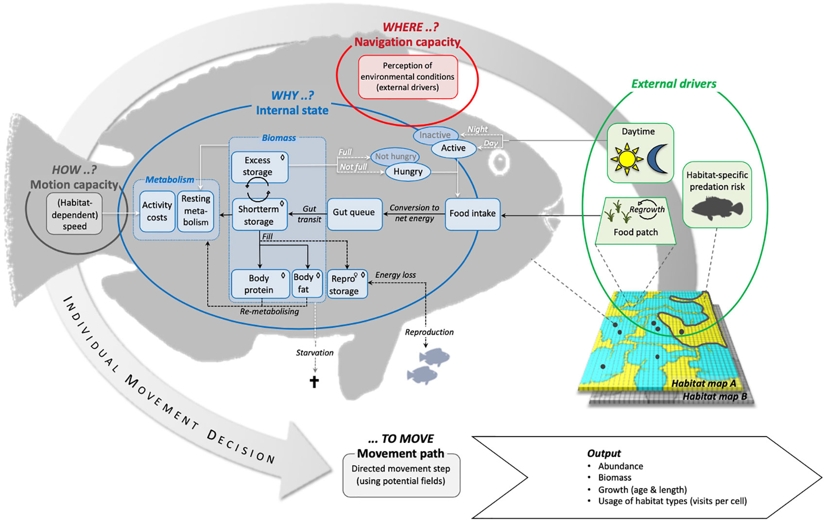
Figure 1 Overview of basic model processes and linkages between model compartments according to the listed components where, how, why … to move in Nathan et al. (2008). → flow of energy, ⇨ flow of information, ⇢ conditional fluxes of energy or information, ◊ compartment size depending on individual body length, ♀ applies solely to female individuals.

To realistically simulate landscape-related movement we incorporate a vector-based movement algorithm that uses artificial potential fields. Potential field approaches are commonly used in computer games and mobile robotics, where they were first introduced by Khatib (1986) and made popular by Arkin and colleagues (Arkin et al., 1987; Arkin, 1989). Based on a physics analogy, these methods treat a (moving) agent as a charged particle acting under the influence of a dynamic magnetic (potential) field representing the current structure of the spatial environment (Connell, 1990; Dudek and Jenkin, 2010). By assigning charges of various magnitudes to all other objects and/or locations in this environment (based on prior knowledge), attractive and repulsive forces are computed navigating an agent in a particular direction. Analogous behaviour can also be perceived in nature, when e.g., reef fishes avoid moving through areas of high predation risk as if ‘repelled’ resulting in the above-mentioned ‘landscape of fear’ (Laundré et al., 2001; Catano et al., 2016). Combined with their mathematical elegance and simplicity (Raja and Pugazhenthi, 2012) this similarity and flexibility make artificial potential fields an appealing approach for the exploration of organismic reactions to landscape structure and its heterogeneity. In our model, the external factors are implemented as attractive (food availability) and repulsive forces (predation risk) thereby acting as the environmental stimuli of the benthic seascape for a fish to move in a particular direction. Behavioural traits such as the formation of harems and/or social groups or territoriality, which are common in reef fish (e.g., Mumby and Wabnitz, 2001; Catano et al., 2015) may also influence movement trajectories of parrotfishes, but were not included in the focus of this study.

With our model we mainly address the following questions: (i) How do small-scale behavioural decisions affect key life history traits such as energy budgets, survival, and the (bioenergetic) ability to reproduce of the model species? (ii) How do these individual decisions influence population dynamics and the spatial distribution as self-organized spatial structures of model species? (iii) What are potential responses on the individual as well as the population level to changing environmental conditions like an increasing habitat fragmentation? (iv) How does the spatial configuration affect energetic gains and costs (e.g., growth and survival)?

2. Material and methods

In this section, we briefly describe the proposed IBM coarsely following the Overview, Design Concepts, and Details (ODD) protocol (Grimm et al., 2006; Grimm et al., 2010; Grimm et al., 2020). A complete model description with detailed model flows, equations, and parameterization along with model validation and the results of the sensitivity analysis is available in Appendix A1 (complete ODD), Appendix A2 (model flow), and Appendix A3 (sensitivity analysis).

Our model has been developed using the object-oriented programming language Java (version 1.8) with the MASON multi-agent simulation toolkit (see https://cs.gmu.edu/~eclab/projects/mason/) and it is available at GitHub (https://github.com/makruse/kitt_model.git). Subsequent data analysis of model outputs is performed using Python 3 with Jupyter Notebook 5.7.4. The model is designed and parameterized based on our field observations of the study system and target organism (unpublished data) as well as the comprehensive literature data available regarding the life cycle, bioenergetics, and general ecology of parrotfishes, in particular the Daisy parrotfish (Chlorurus sordidus) as a ubiquitous and well-studied member of this functional group.

2.1. Purpose

To better understand how the seascape configuration influences small-scale movement decisions of herbivore parrotfishes we developed a spatially explicit simulation model that represents the bioenergetics of individual fishes, their diel movement behaviour, and the resulting population dynamics (Figure 1).

Our specific goals in this study are to assess (i) how trade-offs between effectively foraging and avoiding the risk of predation at the individual level may affect individual growth and energy budgets, as well as the spatial distribution of a population and its (long-term) survival and (ii) whether different habitat configurations with a varying degree of fragmentation may have the potential to enhance or alleviate any of the observed effects. To this end, we simulate six different scenarios with varying spatial compositions and configurations of the benthic seascape (Table 1). The general map structure mimics those of coral reefs encountered during a field study in Northern Sulawesi (Indonesia) and scenarios were constructed keeping the general structure of reef patches with a decrease in cover and increase in fragmentation.

TABLE 1

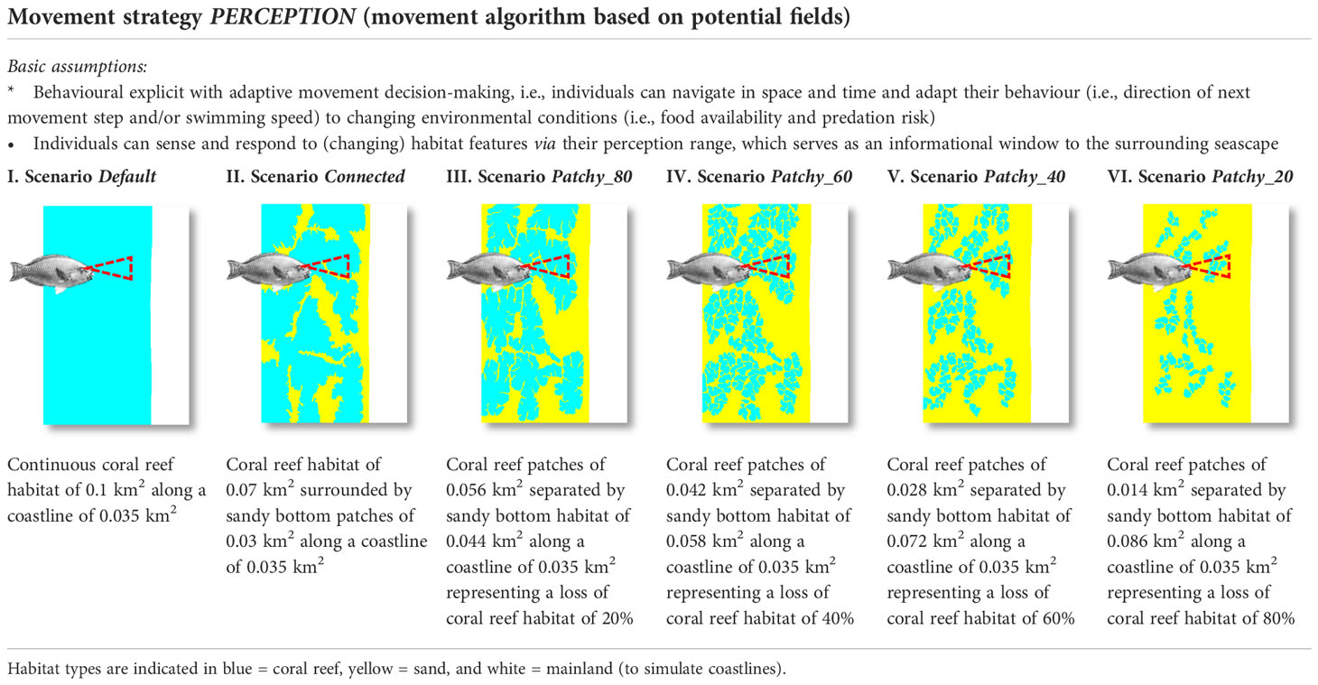
Table 1 Overview of tested scenarios with six alternative seascape settings (I-VI).

2.2. Entities, state variables, and scales

Our model encompasses two entities, the individual reef fish (Appendix A2.1) and the surrounding environment (Appendix A2.2), and three hierarchical levels, the individual, the population, and the underlying benthic seascape.

The model fishes are programmed generically and are here parametrized to represent herbivorous parrotfishes with their coarse life cycle (from post-larval juveniles to adult terminal phases) and bioenergetics following Hölker and Breckling (2005). The state variables of individual fishes (e.g., biomass, length, age) are updated according to a set of rules (behavioural repertoire) including all main activities a fish exhibits during a 24 h cycle such as moving, feeding, growing, reproducing, and resting. Each of the behavioural processes is associated with different energetic gains and costs (in kJ) constituting the model’s ‘currency’ [following Hart (1993)]. A full description of all state variables and execution flows can be found in Table A2.1 and sections Appendix A2.1.1 - A2.1.9.

The virtual environment consists of four principal components to represent the fish-seascape link with its potential key drivers (risk of predation and food availability) for movement decision-making at the spatio-temporal scale of diel movement behaviour: The seascape (HabitatMap) with its food resources (FoodMap), predation risk (PredationRiskFactors), and the time of day (TimeOfDay).

Both, the HabitatMap and the FoodMap are 2D grids of identical size and resolution and constitute the spatial base for the simulation. The FoodMap describes habitat-dependent food resources while the HabitatMap defines the seascape with different habitat types and depicts information on the habitat-dependent predation risk (PredationRiskFactors). The abiotic factor daytime (TimeOfDay) functions as the main controlling force for a fish’s daily activities (Helfman, 1993; Bellwood, 1995). Detailed descriptions, state variables, and parameter settings for all environmental components appear in Table A2.3 and sections Appendix A2.2.1 - A2.2.4.

For our simulation runs, we used an artificial HabitatMap designed to represent typical habitat configurations in tropical coastal environments. The six variants of this map (Table 1) differ in the size of coral reef patches, which are separated by areas of sandy bottom. The coral reef habitat was successively reduced by 20% between scenarios following reported destruction rates, which can be as high as 69% in one year as measured on the Great Barrier Reef after a major bleaching event (Schaffelke et al., 2016). Due to a lack of empirical values with regard to habitat-related mortality rates and computational constraints we model the risk of predation as an increment of the natural mortality rate, which changes depending on the topographic complexity of each habitat type (Pratchett et al., 2008; Welsh and Bellwood, 2012a; McCormick and Lönnstedt, 2013).

The FoodMap holds all relevant information on food availability implemented as an abstract calorific value for epilithic algal turf. We consider this abstract level of the food resource to be sufficient for modelling relevant population dynamics. Algal turf, which is ubiquitous on coral reefs and one of the largest sources of primary production in these systems (Tootell and Steele, 2016), is one of the main food sources of many parrotfishes (Polunin et al., 1995). It is also, however, a food source of low energetic value and parrotfish must therefore continuously feed throughout the day to satisfy their daily energy demands (Chen, 2002). To incorporate feedback processes between individual fishes and the algal food resources we add a regrowth function [following Kelly et al. (2017)].

We set the spatial resolution (grid cell size) to 1 m so that 1 pixel of both, the HabitatMap and the FoodMap, corresponds to 1 m². This reflects the size of a patch that a parrotfish may use in one feeding bout as well as the typical scale comprising a fish’s choice of movement to a new food patch according to field observations of short-term foraging ranges of parrotfishes (Nash et al., 2012; Tootell and Steele, 2016). It also allows the capture of fish movements in detail as well as the representation a fish’s interaction with the surrounding environment based on habitat patchiness or changing spatial distribution of local resources. The simulated landscape equals a total area of 0.135 km² (450 x 300 pixel) encompassing typical home range sizes of < 500 m² of diurnal herbivores like parrotfishes (Welsh and Bellwood, 2012b; Green et al., 2015). Time proceeds in discrete time steps at a high resolution of 1 s to allow for the emergence of habitat-related movement patterns which have been suggested to only be discernible at a narrow range of temporal resolutions (Avgar et al., 2013).

2.3. Process overview and scheduling

2.3.1. Process overview

Our model includes four processes related to a fish’s lifecycle (moving, growing, reproducing, and feeding) and one involving the regrowth of food sources (Figure 2). At every time step each fish can individually evaluate which behaviour is appropriate to the local surroundings and its energy demands to allow for short-term behavioural responses to its internal energetic state.

FIGURE 2

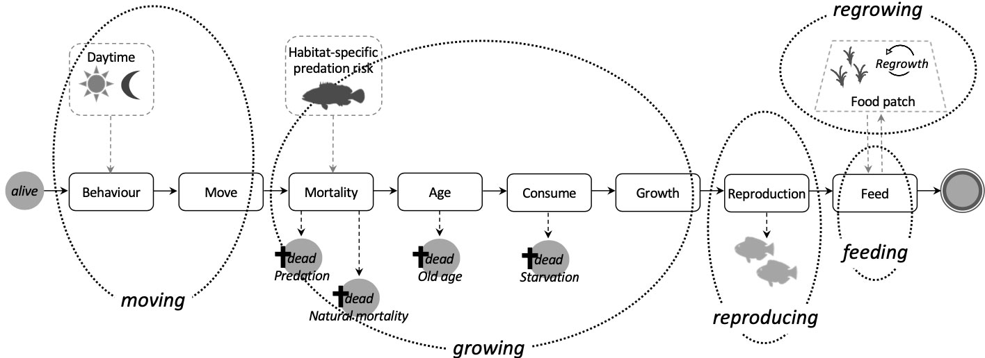
Figure 2 Schematic overview and execution order of main modules and model processes (in italics). Dotted black lines indicate which modules of a fish’s life loop are part of a certain process. Dashed grey lines and arrows illustrate influencing environmental factors.

2.3.2. Scheduling

To mimic a fish’s natural behaviour during a 24 h cycle the scheduling of fish’s activities needed to find a compromise between a biologically meaningful yet computationally practical order. To reflect the overriding and predictable constraint the diel cycle imposes on the behaviour and activity of fishes (Helfman, 1993) we implement the factor TimeOfDay (Appendix A2.2.4) which primarily controls a fish’s behaviour (Appendix A2.1.2). Parrotfishes like C. sordidus as diurnal herbivores spend on average about 90% of daylight hours foraging with abruptly starting and stopping to feed at dawn and dusk (Bellwood, 1995). At dusk, they move to boulders or rocks on the reef slope to sleep (Bellwood, 1995). Though feeding activity of parrotfish might vary over the course of the day (Bellwood, 1995; Zemke-White et al., 2002), we use a simplified, i.e., constant influence of the diel cycle to maintain efficient model computation. Thus, depending on TimeOfDay our diurnal model fish either forage, rest or migrate from resting to feeding habitats or vice versa.

A model fish with the status of active and hungry will move to search for food based on a spatially informed movement algorithm (for this we use the concept of potential fields described below and in detail in Appendix A2.1.3). On a food cell a fish will deplete the resources according to its body-size-dependent feeding rate (meanIngestionRate) until it has gained enough energy to meet its energetic demands (Appendix A2.1.9). The model uses individual energy budgets for each fish to describe the partitioning of the ingested energy into metabolic processes, deposited as new body tissue (including reproduction), or lost as waste products (Willmer et al., 2005)

In case more energy is consumed than assimilated the fish will eventually die because of starvation. All assumptions underlying the allocation and conversion of energy are detailed in Appendix A1.2 and A2.1.6-A2.1.9 with all related parameters listed in Table A2.2.

Apart from starvation, a model fish can also die due to predation (Appendix A2.2.3), senescence (Appendix A2.1.5), or due to background mortality (Appendix A2.1.4). In the DEFAULT scenario all types of mortality are implemented to approximate a total annual mortality rate of 0.3 to 0.4 year^-1 without fishing as fishing mortality is not (yet) implemented in our model.

Individual fishes are referred to either as juveniles (considered as non-reproductive females), females, or males. C. sordidus is a protogynous species and we thus include female-to-male sex change in our model. This is important because ignoring life history variation in assessing stock dynamics has been demonstrated to lead to an overestimation of spawning biomass (Alonzo et al., 2008). Female fishes in their initial phases can spawn as soon as they have acquired enough energy resources in their reproduction storage (Appendix A2.1.8). Spawning can occur during each time step as parrotfishes like C. sordidus are known to spawn daily and throughout the year with no clear seasonal patterns (McIlwain and Taylor, 2009). Following Lewis (1997), Miller et al. (2001) and Miller and Kendall (2009) and to ensure a stable (self-recruiting) model fish population over time we assume that two juvenile individuals per female and spawning event (NumRecruits) settle within the population after the timespan of a post-settlement age of 120 days had passed [following McIlwain and Taylor (2009)].

2.3.3. Movement

To navigate through its surroundings a model fish can make an informed movement decision based on perceived environmental conditions regarding food availability and predation risk. At each time step, the actual movement step is modelled discretely using a vector-based swimming algorithm based on the step length (defined by the current speed) and the turning angle (direction). The direction (in degree) is computed using artificial potential field algorithms (see Appendix A2.1.3 for details) and constrained by a maximum turning range and a spatial perception range, while the actual speed value (in cm s^-1) is determined by the fish’s current activity and the underlying habitat type.

To realistically depict a fish’s response toward the seascape characteristics we incorporate a perception radius for each relevant habitat feature. This radius functions as a spatial range, in which a fish will react to a certain feature and include it in its movement decision. For the risk of predation, we set the perception range (perceptionRadiusPredation) to 10 m (Myrberg and Fuiman, 2002). For computational reasons the inclusion of the dynamic habitat feature food availability in the decision-making process is limited to the next eight directly adjacent cells. These neighbouring cells represent the perception range (perceptionRadiusFood, [m]) of a model fish implying a reactive distance of 1 m (see Appendix A1.3 and A2.1.3 for further details). Moreover, fishes are not only known to be able to sense changes in predation risk or food availability in different habitats but also to adapt their velocity accordingly (Milinski, 1993). Therefore, a model fish will not only adapt its movement direction according to the perceived surroundings but also increase its speed in riskier (i.e., topographically less complex) and/or low-food habitats (SANDYBOTTOM_SPEED_FACTOR) and become slower under more favourable conditions, i.e., habitats with high structural complexity (Nash et al., 2012; Nash et al., 2016; Tootell and Steele, 2016) and/or high food availability. Details on the exact computation of movement steps appear in Appendix A1.3 and A2.1.3.

2.4. Design concepts

2.4.1. Objectives

The foremost goal of each fish is to ensure its survival by meeting its energetic requirements. To achieve this objective a model fish will try to reach the (theoretical) biomass it would have gained at its current age under ideal conditions based on the species-specific Von Bertalanffy Growth Function, one of the most widely used growth curves in fisheries science (Appendix A2.1.6).

2.4.2. Emergence and adaptation

All properties on higher integration levels such as population or the status of the environment result in a self-organised way from the interaction of the parts on lower levels (see Reuter et al., 2005, Figure 1). The population level (e.g., population size, length-, age-, and life-phase distributions) as well as its spatial distribution arise from the properties of the individual fishes regarding their ontogenetic development, somatic growth, and movement behaviour(s) as well as direct interactions with the underlying seascape structure.

Furthermore, the resulting performance and processes of the individual such as the movement pattern or mortality are not modelled directly but emerge from the specific state of an individual and the status of its direct environment. Concerning movement, this includes a fish’s energetic level and relevant habitat information (resource level) while regarding mortality, its current age, possible failure to keep a minimum energetic level or the time spent on a particular habitat combined with the habitat-related predation risk can be decisive.

In the context of specified behaviour, a fish is capable of making adaptive decisions based on its internal state and the status of the environment. For instance, a fish will increase its feeding rate the more its energetic state diverges from the desired state. This behaviour follows Godin (1981) as fish are known to be able to increase their average feeding rate with increased hunger levels. Furthermore, fish enhance the chance of survival by adapting their direction of the next movement step to the most favourable position regarding predation risk and/or food availability.

2.4.3. Sensing

Information on the environment influences the activity a model fish executes. However, through the implementation of a perception range the information, that a fish can perceive, is restricted to the local environment. Individual fishes also ‘know’ their internal states such as the energetic or reproductive state. Both, the environmental and internal information are then considered in the decision for a specific activity.

2.4.4. Stochasticity

Stochastic events in our model include the selection of swimming speed and choice of movement direction when the fish is moving at RANDOM as well as life phase transitions and whether a fish will die due to predation or natural causes like diseases. Furthermore, during initialization the initial age and position on the habitat grid are assigned randomly to each fish as well as the initial standing crop to each grid cell of the food map (Appendix A1.4.5 and A2.2.2). Any recruit that enters the simulation after a spawning event will also be placed randomly on the simulation grid. Moreover, the order in which individual fishes and their scheduled activities are processed is generated randomly.

2.4.5. Observation

Our model keeps track of the fate of the individual fish including location and energetic state. On the population level, the model calculates the total abundance and biomass, the abundances and biomass grouped by life phase (juveniles, females, males), as well as age- and size-frequency distributions at regular pre-defined intervals. On the environmental level, it records the number of fish visits that occur in each habitat cell over a predefined period to allow for an analysis of habitat use patterns and spatial distributions of fishes across the simulated seascape (Table A2.3).

2.5. Initialization

The initialization process starts with the habitat grid as the virtual environment for the fish population. During initialization each grid cell is assigned a habitat type based on an external input file and a random food value within the limits of its habitat type. This is followed by the calculation of the potential field based on habitat type and resource level. Due to computational constraints, the habitat grid is initially occupied with a population of 50 randomly placed individuals, whose initial age distribution is derived stochastically from (arbitrary) probabilities given for each maturity state. The other individual state variables like biomass and body length are then computed accordingly based on the implemented formulas and assumptions summarized in Appendix A2.1. A simulation starts at 8 hrs and DAYTIME as TimeOfDay, when parrotfish usually start feeding.

2.6. Input data

The model has been constructed modularly with different input files specifying the general setting, the simulated species, and the environment. Each of these files can be replaced to automatically run different scenario configurations. Input files are:

● a configuration file specifying general simulation settings (duration of simulation run, initial population size, further input files, etc.)

● a. png using a predefined colour code to specify the habitat configuration of the underlying seascape

● a. xml file with key life history parameters to specify simulated fish species

2.7. Model validation

Our model is parametrized, tested, and validated following a hierarchically structured validation approach (Reuter et al., 2011; Kubicek et al., 2015). For parametrization, we mainly use information from three different sources: Experimental data, expert knowledge including own field observations of the study system and target organism (unpublished data), and calibration. Most of the parameter values are directly obtained from published field studies on parrotfish and reef ecosystems, while parameters concerning the recruitment rates and habitat-dependent predation risks are estimated based on available literature regarding general reproduction patterns of reef fish and overall natural mortality rates, respectively. We further set the values of the pathfinding weighing factors, for which presently no data is available, based on studies regarding the relative importance of different habitat-related drivers for fish movement and our expert knowledge of the study system gathered during several years of field research. To assist parametrization and calibration of parameter values which are highly uncertain (no data available or known to be difficult to estimate) or to which we suspect model outputs to be highly sensitive we conduct a sensitivity analysis (Reuter et al., 2011). To do this, we identify the most susceptible parameters of each main model process (food availability, movement, energy gain and loss, reproduction, and survival), cover the biologically plausible range of each of these parameters by varying each parameter one at a time by ± 10%, and simulate all potential combinations with three different seeds each (i.e., three replicates per parameter combination). We then evaluate the effects of changing parametrization on population metrics like total biomass, abundance, and life-phase ratios as critical model outputs.

To assess the validity of our model and its parameter settings, i.e., the robustness, precision and reliability of model results (Reuter et al., 2011) we inspect the energetic state of the individual fish process by process and by defined variables that can be compared to available independent data such as the body weight and length. These quantities contain information relative to growth, reproduction, and survival we aim to interpret concerning habitat-dependent movement behaviour and space use patterns. On the population level, we assess the (long-term) population structure that emerge from the interactions of the individuals regarding abundances, biomass, age-distributions, life phase composition and reproduction frequency and compare them to published field observations. Our model validation is further assisted by an appropriate choice of output plots monitoring population dynamics.

By performing this consistency check of key processes and dynamics on different hierarchical levels we ensure that the system behaviour we intend to represent has been captured correctly and results are reliable within the applied conceptual system (Reuter et al., 2008). Based on this data reconciliation and visual inspection of model outputs with results from the literature we then choose the parameter set that can reproduce a realistic population structure for our subsequent simulation experiments. Details on model validation and results of our sensitivity analysis can be found in Appendix A3.

2.8. Simulation experiments

To assess whether and how individual development and population dynamics are influenced by individual capabilities to interact with the environment and/or habitat settings (habitat configuration and level of fragmentation) we conduct a series of simulation experiments: We test six different scenarios (Table 1) with each factor combination replicated three times. Each replicate simulation is run for a time limit of 30 years and a maximum population size of 175 individuals (for computational feasibility). The time period modelled encompasses several generations thereby allowing for conclusions on a population level. The evaluation of a simulation run starts from Year 10 as the first year in which the number and life-phase ratios of model fishes is comparable to those of parrotfish populations observed in field studies (see Appendix A3 for details).

3. Results

3.1. Fish abundances, biomass, and life phase composition

There are substantial differences in the total abundance, biomass, and life phase compositions of model fish populations among simulations under different scenarios (Figure 3). While the two scenarios Connected (connected reef habitat of 0.07 km²) and Patchy_80 (reef habitat patches of 0.056 km²) differ relatively little compared to model results of the Default scenario (continuous reef habitat of 0.1 km²), both the scenarios Patchy_40 (reef habitat patches of 0.028 km²) and Patchy_20 (reef habitat patches of 0.014 km²) show a high and increasing decline in fish abundance (Patchy_40 = ~40%, Patchy_20 = ~90%, Figure 3A) and biomass (Patchy_40 = ~45%, Patchy_20 = ~85%, Figure 3B). Fish populations under the scenario Patchy_60 (reef habitat patches of 0.042 km²) initially develop similarly to the Default scenario but begin to decline in biomass and abundance from Year 15 onwards and level off at a value of 85% (abundance and biomass).

FIGURE 3

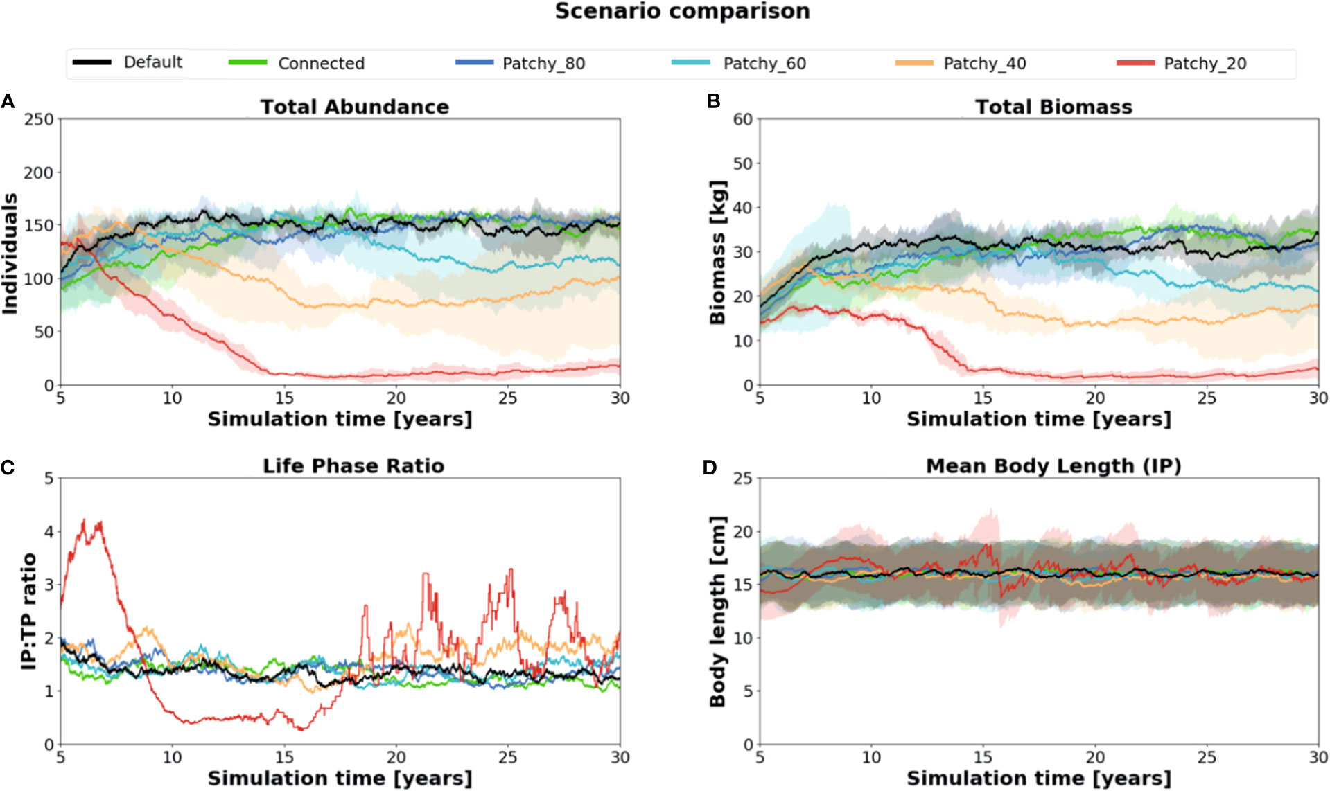
Figure 3 Comparison of key population characteristics of simulation runs under different scenarios: (A) total abundance, (B) total biomass (C) life phase composition (IP : TP), and (D) mean body length of (female) fishes in their initial phase (IP). Standard deviation is indicated as shaded areas around the mean.

Of all simulated scenarios the Initial Phase (IP):Terminal Phase (TP) ratio varies strongest in scenario Patchy_20 with values as high as 4.3:1 and as low as 0.2:1 (Figure 3C). Populations thus change from being strongly female-dominated to more male-dominated during the simulation period and eventually oscillate between 3.2:1 and 1.1:1. In all other scenarios the IP : TP ratio is rather stable throughout the simulation period and settles at a value of about 1.4:1 indicating a balanced ratio between female and male model fishes with a slight tendency to an increased number of females.

Initial-phase females, which control recruitment and thus have a key function in regulating model population dynamics, have a mean body length of about 16.0 cm (Figure 3D). Again, the value varies most strongly in the Patchy_40 and Patchy_20 simulations but is similar across all other simulations suggesting that in these scenarios female fishes can still acquire enough energy to maintain their individual growth.

Total abundances in the Default scenario with on average 150 ± 10 fishes (Figure 4A) are comparable to those of the scenarios Connected (150 ± 9 fishes, Figure 4B) and Patchy_80 (148 ± 14 fishes, Figure 4C), but approximately 15% higher compared to Patchy_60 from Year 15 onwards (125 ± 31 fishes, Figure 4D), about 2-fold higher compared to Patchy_40 (88 ± 38 fishes, Figure 4E), and about 9-fold higher than under scenario Patchy_20 (17 ± 6 fishes, Figure 4F).

FIGURE 4

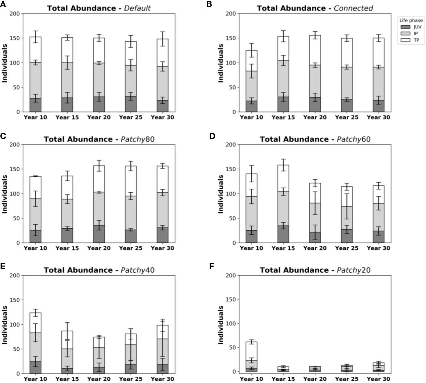
Figure 4 Abundances and life phase composition of model fish populations at different points in time during a simulation under different scenarios: (A) scenario Default, (B) scenario Connected, (C) scenario Patchy_80, (D) scenario Patchy_60, (E) scenario Patchy_40, and (F) scenario Patchy_20. Bars indicate mean values (± standard deviation (SD)) and are subdivided into life phases (JUV = juveniles, IP = (female) initial phases, TP = (male) terminal phases).

As mentioned above life phase compositions vary little throughout the simulation period under the Default scenario with on average 28 ± 6 fishes in the juvenile phase, 69 ± 7 in their (female) initial phase (IP), and 53 ± 10 in their (male) terminal phase (TP). Very similar compositions can be found in simulations under the scenario Connected (28 ± 6 juveniles, 69 ± 7 IPs, 54 ± 8 TPs) and Patchy_80 (29 ± 7 juveniles, 68 ± 8 IPs, 52 ± 9 TPs). Ratios under the scenario Patchy_60 start to deviate from the Default scenario after ~15 years (23 ± 10 juveniles, 58 ± 19 IPs, 43 ± 9 TPs) with a tendency to more female dominated populations as fewer individuals reach their terminal phase. Proportionally even fewer male fishes are present in the simulations under scenario Patchy_40 (16 ± 10 juveniles, 44 ± 22 IPs, 28 ± 10 TPs). As mentioned above under scenario Patchy_20 proportions of life phases are highly variable with on average 3 ± 2 juveniles, 6 ± 3 IPs, and 8 ± 3 TPs.

3.2. Mortality rates and reproduction frequencies

Total annual mortality rates (Figures 5A–F) change little between scenarios (Default = 0.278 ± 0.071, Connected = 0.259 ± 0.065, Patchy_80 = 0.271 ± 0.067, Patchy_60 = 0.270 ± 0.080, Patchy_40 = 0.272 ± 0.104), except for scenario Patchy_20 with 0.347 ± 0.248. In addition, little variability can be observed in the relative contribution of the different types of mortality, which range on average between 0.105-0.131 (M_nat), 0.116-0.130 (M_pred), and 0.032-0.085 (M_age). In contrast to mortality rates, there is considerable variation in the reproduction frequency among the different scenarios from on average 20 to 24 reproduction events per year (Default = 24.0 ± 4.1, Connected = 23.7 ± 4.4, Patchy_80 = 23.5 ± 5.6, Patchy_60 = 20.7 ± 8.8), to values as low as 2 to 12 (Patchy_40 = 11.5 ± 6.8, Patchy_20 = 2.1 ± 1.2). With relatively stable mortality rates across scenarios and declining reproduction frequencies, which cannot compensate losses due to mortality, populations will inevitably collapse and eventually become extinct. As female fishes are mostly able to maintain their individual growth (with the exception of scenario Patchy_20, see above), but increasingly lack the energy to reproduce, the modelled systems seemingly become more and more food-limited. Moreover, reproduction seems to be the model process most susceptible to an increasing fragmentation and loss of habitat, rather than affecting population survival due to a growing risk of predation.

FIGURE 5

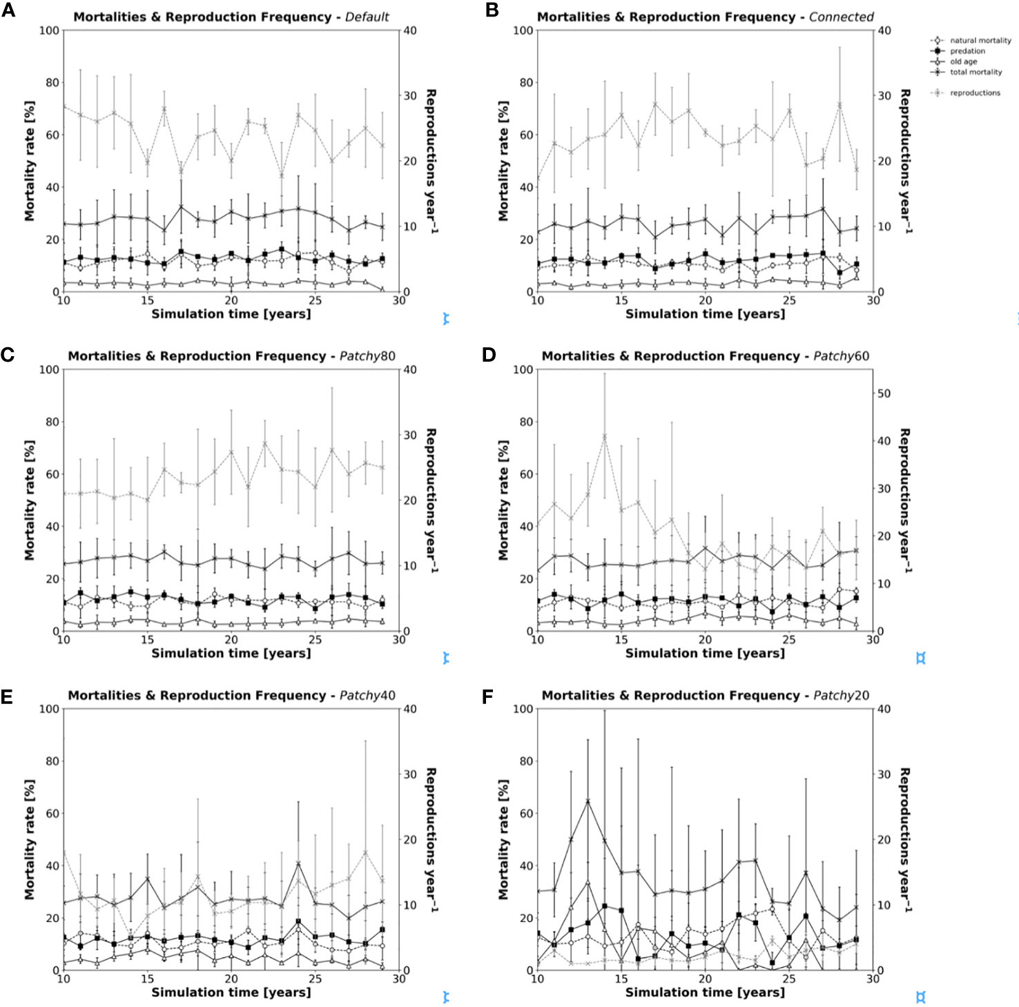
Figure 5 Annual mortality rates (in black) and reproduction frequency (grey dashed line) of model fishes during a simulation under different scenarios: (A) scenario Default, (B) scenario Connected, (C) scenario Patchy_80, (D) scenario Patchy_60, (E) scenario Patchy_40, and (F) scenario Patchy_20. Values are mean values (± standard deviation (SD)) of replicated simulation runs.

3.3. Individual space use and spatial distribution of the fish population

Individual movement trajectories over 20 min differ noticeably across scenarios (Figure 6) and the shape of the short-term foraging range changes with the availability and distribution of coral reef habitat: As the coral reef habitat increases the more circular the movement becomes (Figure 6A). Consequently, the linear distance travelled increases in dependence on the area of sandy bottom a fish has to cross to reach more favourable coral reef habitat patches (Figures 6B–F). In the examples shown in Figures 6A–F the distances travelled during a 20 min period increase from approximately 40 m in continuous reef habitat to 75 m in a highly fragmented reefscape, which corresponds to an increase of ~190%.

FIGURE 6

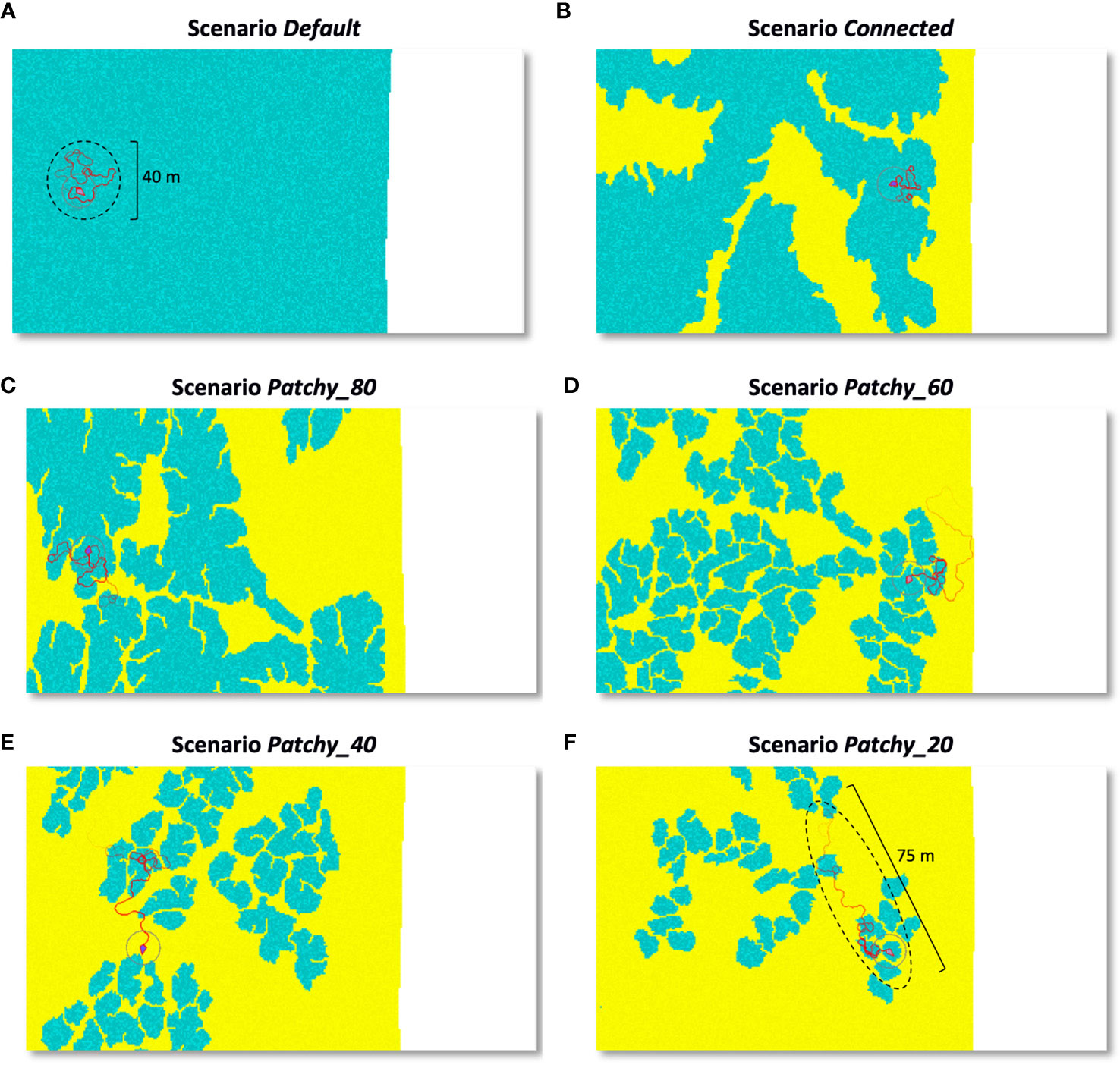
Figure 6 Individual movement trails of a (female) model fish in its initial phase over a 20 min time period and under different scenarios: (A) scenario Default, (B) scenario Connected, (C) scenario Patchy_80, (D) scenario Patchy_60, (E) scenario Patchy_40, and (F) scenario Patchy_20. Blue areas = coral reef habitat, yellow = sandy bottom, white area = coastline. Darker shades of a colour indicate higher food availability and circular areas illustrate the fish’s perception radius.

The emerging patterns of the spatial distribution of modelled fish populations are not uniform among the tested scenarios (except the Default scenario with only one habitat type, Figure 7A) but reflect the distribution and configuration of the coral reef patches of the underlying seascape (outlined in light grey, Figure 7B). While the monthly space use pattern under the scenario Connected (Figure 7B) appears relatively homogenous among coral reef patches, the frequency of visits is concentrated among certain patches in all other scenarios. Under the scenario Patchy_60, for instance, some patches in the upper region are heavily frequented (Figure 7D) with > 8000 visits per cell, a tendency that is even more pronounced under scenario Patchy_40 with values of > 9500 visits per cell (Figure 7E). This pattern is also well visible in the visit frequency per grid cell (normalized for one fish) shown in the histograms of Figures 7A–F. While under scenario Default, Connected, and Patchy_80 the number of visits per grid cell range between 0-80, the visit frequency increases by one order of magnitude under the scenarios Patchy_40, Patchy_60, and Patchy_20. Interestingly, under all scenarios except Default and Connected some of the coral reef patches are hardly visited at all throughout the period of one month. In general, however, space use patterns seem to be driven by the characteristics of the underlying habitat structure.

FIGURE 7

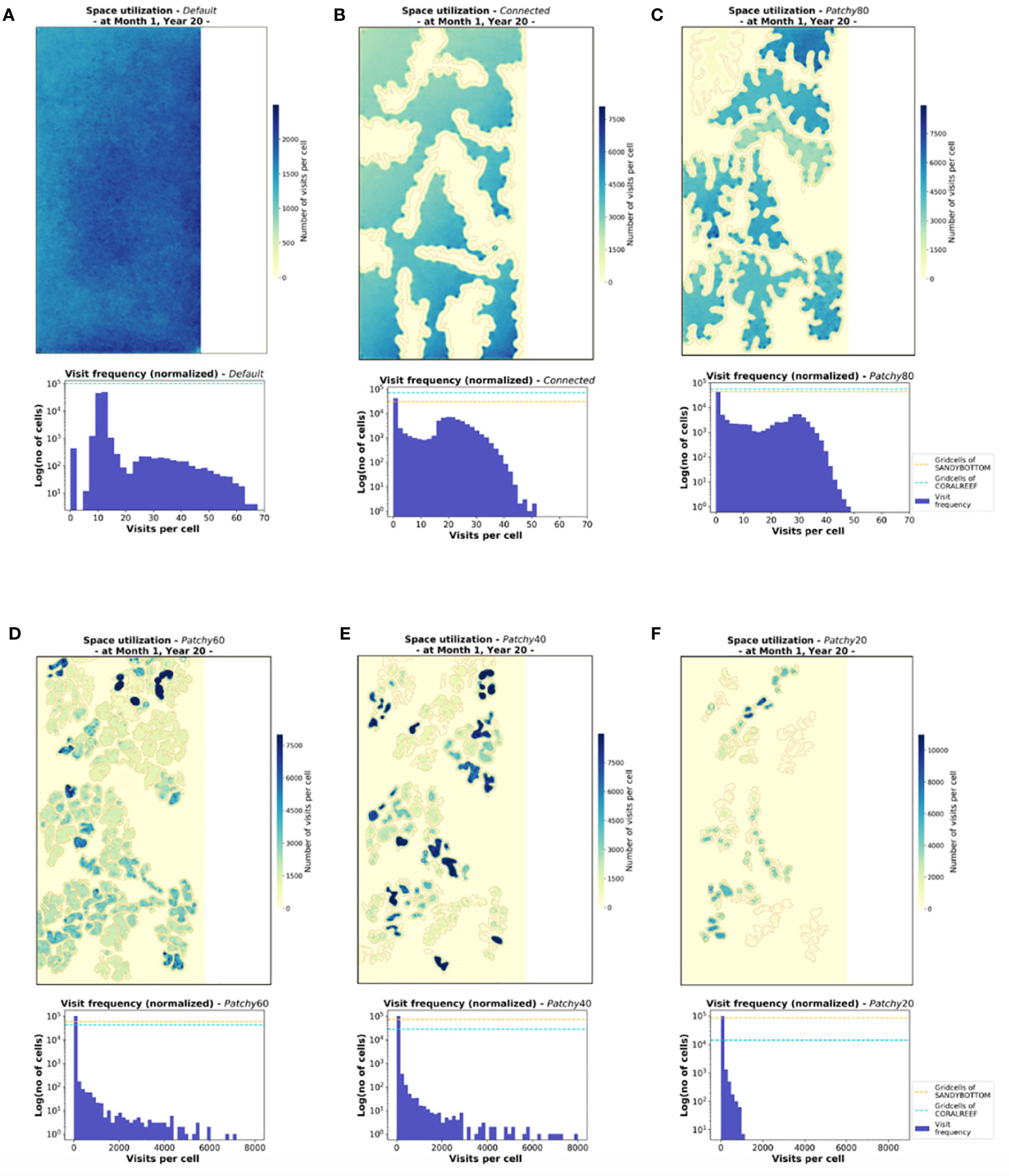
Figure 7 Cumulated visits of fishes to each habitat cell illustrating the monthly space use patterns on the population level for the six different scenarios (A-F). Shown are heatmaps and histograms of visit frequency per grid cell (normalized for one fish), both based on representative data of Month 1 at Year 20 of the simulation period. The underlying patches of coral reef habitat are outlined in light grey, gird cells of type MAINLAND are indicated in white (heatmaps). Histograms display visit frequency to the habitat cells CORALREEF and SANDYBOTTOM (without MAINLAND cells) and proportions of the two habitat types are indicated by dashes lines.

4. Discussion

Our simulation experiments reveal substantial differences on both the individual and population level between the six scenarios tested (Default, Connected, Patchy_80, Patchy_60, Patchy_40, and Patchy_20), in which the underlying coral reef habitat is increasingly fragmented and successively reduced by a rate of 20%. Based on annual rates of coral reef destruction, which can be as high as 69% (Schaffelke et al., 2016), our scenarios thus represent situations, that may occur in coral reef systems throughout relatively short periods of a few years or less. While the scenarios Default, Connected, and Patchy_80 show similar developments, the scenarios Patchy_40 and Patchy_20 deviate strongly in their results with Patchy_60 exhibiting intermediate trends. In general, our findings reflect the outcomes of empirical studies in various aspects and elucidate the potential of seascape characteristics to guide and constrain the movement of herbivorous fishes.

4.1. Population dynamics

The modelled fish populations respond as expected to the manipulation of habitat configurations and degree of fragmentation regarding abundance, biomass, and overall survival. Population size declines gradually among scenarios along with food-rich and safer coral reef habitats. A loss of reef habitat by 80% (scenario Patchy_20) corresponds to a reduced fish abundance by almost 90% compared to the scenarios Default and Connected. Apart from the loss of the coral reef itself, the subsequent decline in parrotfishes may have further adverse effects on the ecosystem functioning as parrotfishes are important bioeroders and structuring forces for benthic communities (Bellwood, 1995; Bonaldo et al., 2014; Welsh and Bellwood, 2014). By keeping turf algae in a cropped state parrotfish provide an open substrate for enhanced coral recruitment and thereby have the potential to mediate coral-algal dynamics (Mumby et al., 2006; Hughes et al., 2007; Russ et al., 2015; Tootell and Steele, 2016; Roff et al., 2019). A change in these complex interrelations may further alter an ecosystem’s ability to respond to disturbances (Bellwood et al., 2004).

Interestingly, the decline in model population size is mainly caused by a reduced reproduction frequency rather than an increase in predation mortality (except scenario Patchy_20) and/or starvation. This decrease can be caused by both the reduced total number of females and a decrease in energy gain due to the reduction of food-rich coral reef habitat. As predation mortality in our model is determined by habitat complexity combined with the time spent on risky habitats and a fish can react to changing predation risk by changing its movement direction and thereby reduce the time spent on riskier habitats, it seems plausible that predation mortality does not increase significantly among scenarios. However, as indicated by predation mortality rates under scenario Patchy_20 increasing distances moved over low complexity and riskier habitats will inevitably result in increased exposure to predation, as was also demonstrated in field experiments of different herbivore fishes including C. sordidus (Madin et al., 2010; Madin et al., 2011).

In general, total annual mortality rates, which change relatively little between scenarios and vary between averages of 28% (scenario Default) and 35% (scenario Patchy_20), compare very well to those reported by Gust et al., (2002) with annual mortality estimates ranging from 28% to 43% for C. sordidus populations. Also, sex composition ratios (IP : TP) ranging from 3.2:1 to 1.1:1 within the different scenarios are in a similar order of magnitude as values reported for unfished populations of C. sordidus from 4.75:1 on the mid-shelf to 1.48:1 on the outer shelf of the Great Barrier Reef (Gust, 2004).

The reason that model fishes do not experience mortality from starvation (as an emergent property) in our simulation experiments is likely to be caused by the low density of the model population, which is 4- to 6-fold lower than observed in the field (due to computational constraints, see Appendix A3.2). However, model results clearly show that even though female fishes can maintain their individual growth, they increasingly lack the energy reserves to be able to reproduce, indicating a growing food limitation of the model system. As reproduction is known to be the most metabolically demanding activity in the lives of fishes (McBride et al., 2015) it is not surprising that reproduction proves to be the model process most susceptible to changes in habitat configuration and composition, and hence food availability. These findings are in accordance with field studies of C. sordidus made by Tootell and Steele, (2016), in which individual energy reserves decreased with algal turf resources suggesting that resource availability is an important factor determining the physiological condition of this species. Moreover, a decreased reproductive output will not only have implications for the persistence of the local population but may also negatively affect the neighbouring population by a reduced supply of recruits. Apart from having a direct influence on the number of offspring a female may produce, empirical evidence exists that the amount of energy a female has available to invest into egg production will also affect egg quality, and this in turn the offspring’s fitness (Bagenal, 1969; Crespi and Semeniuk, 2004; Berg and Fleming, 2017).

4.2. Movement behaviour and space use patterns

To better understand the consequences of population distributions and the constraints on ecosystem functions it is important to determine how individual fishes use the space when foraging and what factors may influence their movement decisions and hence their mobility (Nash et al., 2012). In the scenarios examined linear distances travelled per unit time grow longer (up to 190%) and the shape of the foraging range is more elongated (see Figure 6) the more fragmented the coral reef habitat becomes. This behaviour change is also found in nature as, when habitat fragmentation increases, individual fishes will have to travel over larger areas per unit of time to reach suitable foraging sites, to maintain their energy intake rates. Our findings are in accordance with field studies of parrotfish foraging behaviour by Nash et al. (2012), in which high levels of coral cover corresponded to more compact and circular short-term foraging ranges for two common parrotfish species, Scarus niger and S. frenatus.

The implications of this change in foraging behaviour can be 2-fold. Firstly, the longer the distances an individual fish has to swim the higher its energetic costs. Moreover, a fish will also increase its swimming speed when moving over an unfavourable habitat (Milinski, 1993), which further adds to its energy expenditure. With more energy spent on swimming longer distances (Figure 6), the fish has less energy left to invest in somatic growth and/or reproduction. Differences in surplus energy may also have consequences for processes such as tissue repair and maintenance or defence against predators and the trade-offs between movement, growth, and reproduction are often at the expense of the reproductive output (Goldstein et al., 2017). Thus, habitat fragmentation is most likely to strongly influence the energy budgets of female fishes and their spawning frequency as shown by our model results and discussed above.

Secondly, with changing spatial dimensions of their foraging range individual fishes will cover different areas during their daily routines. Hence, parrotfishes seem to be able to make small-scale changes in their movement behaviour in response to the loss of coral reef habitat and their control of algal turf growth might be reduced and/or occur over different spatial ranges. This has also been observed in the field by Gil et al., (2017), who showed in their investigation of herbivory in French Polynesia that the fragmentation of refuge habitat resulted in a reduction of the consumer’s control of food resources.

Concerning the structuring force of herbivore organisms, a change in individual space use patterns becomes even more relevant on the level of the population as the consequences of grazing depend in part on spatial abundance patterns (Mumby et al., 2006; Paddack et al., 2006). Model outputs reveal that the spatial distributions of fish populations (emergent as the cumulative behaviour of the individuals and illustrated above as the average number of visits per cell cumulated over one month) closely reflect the seascape arrangement. By concentrating their foraging activity within the coral reef patches model fishes graze in a spatially constrained manner. Model results are thus in accordance with recent findings over similar spatial scales by Madin et al. (2019): Their daytime remote video surveys demonstrated that herbivorous fishes spend dramatically more time closer to the shelter of reef patches than in the adjacent sand flat habitat. In their study, no herbivores were observed beyond rather small distances of 7.5 m and grazing intensity was hence highest close to the reef. By 15 m from the reef, no grazing by herbivores could be recorded. As indicated by our simulation results these field observations also suggest the existence of a behavioural constraint that spatially restricts herbivore foraging patterns.

Intriguingly, our simulation experiments also show that with an increasing habitat fragmentation coral reef patches are less equally frequented with an intensified foraging effort on specific patches and others rarely visited throughout the duration of one month. This concentration of foraging effort again has implications for the ecosystem function provided by the parrotfishes, as the grazing pressure will be more intensive in some patches and substantially lower in others. Furthermore, the irregular usage of different reef patches may also have consequences concerning the social relationships among individual parrotfishes as it can affect encounter rates with conspecifics and/or competitors. Thereby the ‘effective’ distance between individuals may be much larger than their physical distance, a landscape property detailed in the much-debated concept of ‘landscape connectivity’ (Taylor et al., 1993; Taylor et al., 2006). However, as density-related processes are not yet explicitly considered in our model further simulation experiments and model adaptations will be necessary in the future to investigate this aspect more thoroughly. Nonetheless based on our findings and as stated by others (e.g., Nash et al., 2012) it appears advisable to incorporate behavioural flexibility when representing herbivory in time and space. The more accurate our estimates the more we will be able to better understand how coral cover might be affected on a local scale or why shifts in community compositions occur.

4.3. Landscape of fear

Risk effects are known to alter habitat and space usage of prey organisms (Madin et al., 2012; Manassa et al., 2013; Madin et al., 2019) and can be visualized in the model of the ‘landscape of fear’ established by Laundré et al., (2001). In this model the relative levels of predation risk that a prey organism experiences in different areas of its environment are represented as peaks and valleys (Laundré et al., 2010). We incorporate this concept in our model using a novel approach that combines individual-based modelling with artificial potential field algorithms: To this end, we translate the peaks and valleys of the (habitat-related) predation risk into a potential field map in which a growing risk of predation is represented as increasingly repellent areas. As ample evidence exists that predation risk correlates with habitat types and characteristics such as topographic complexity (Lima and Dill, 1990; Jones and Syms, 1998; Chapman and Kramer, 2000; Overholtzer-McLeod, 2006; Pratchett et al., 2008; Turgeon et al., 2010; McCormick and Lönnstedt, 2013; Catano et al., 2016; Roff et al., 2019), we correlate the habitat structure with the perceived risk of predation. This information is then used by the individual fishes and included in the decision-making process for the direction of the next movement step. In our simulation experiments, individual fishes react to elevated predation risk by avoiding risky areas and/or by less tortuous movement paths to minimize the time spent on riskier habitats. Our results thus support empirical studies showing that spatial areas of high risks are less likely to be grazed and areas of lower risks are at elevated risk of disproportional high grazing intensity (Madin et al., 2010). As suggested by Laundré et al. (2001) behavioural responses to different levels of predation risk may therefore have more far-reaching consequences for the systems under consideration than the actual killing of individuals by the predators. However, evidence also exists that while the loss or fragmentation of refuge habitat reduces consumer control of resources, greater resource densities may counteract this effect by altering landscapes of fear of consumer species (Gil et al., 2017). Furthermore, habitat degradation may also lead to an increase rather than a decline in resource density as bleached corals, for instance, are known to become over-grown with turfing algae (Diaz-Pulido and McCook, 2002; O’Brien and Scheibling, 2018). To be able to evaluate potentially counteracting effects due to resource availability by our model, it will be necessary to include further habitat types and/or scenarios with diverging properties as food density and predation risk change in the same direction in the two implemented habitat types CORALREEF and SANDYBOTTOM. Two other aspects would have been particularly interesting to explore, and we believe they are promising future extensions of our model: the interaction between conspecifics to depict social organisation such as territorial behaviour or harem formation, and the inclusion of a predator species to model consequences of individual prey-predator interactions. Parrotfish are known to display social behaviour and male parrotfishes commonly hold female harems in territories or gather in mixed-sex groups (Mumby and Wabnitz, 2001; Afonso et al., 2008; Catano et al., 2015). These social factors appear to have an impact on the size of home range excursions (Welsh et al., 2013) and group fish have shown to conduct larger movements than territorial fish (Afonso et al., 2008). Depending on the behavioural strategy space use pattern of the fishes could therefore differ and might ultimately alter the survival rate of a population in highly fragmented habitats. Moreover, the explicit modelling of conspecific interaction would allow us to depict the potential reliance on proximity of (male) conspecifics to initiate a spawning event (Sancho et al., 2000). Given that the IP : TP ratios in the scenarios with very high habitat fragmentation (Patchy_40, Patchy_20, see Figure 3) indicate populations to be more female dominated, reproductive events could potentially become rarer and might further stress the sensitivity of reproductive processes towards habitat fragmentation. Inclusion of a predator species would allow for an investigation of patterns reflecting individual prey encounters with individual predators (i.e., acute predation risk). Under increasing acute predation risk parrotfish like C. sordidus have been shown to take significantly shorter excursions highlighting the decisive influence of prey-predator interactions on herbivore movement behaviour (Madin et al., 2012).

Due to its structure and modular composition, the above-mentioned adaptations are relatively easy to implement in our model. Moreover, the integration of artificial potential field algorithms offers a simple mechanism to include directional decisions based on habitat configurations as our results indicate. The possibility to adapt the model to a wide range of (reef) fish species via the life-history related parameters combined with the option to specify habitat configurations via custom habitat maps further allow for an evaluation of various local settings and scenarios. Our model thereby provides a generic approach that incorporates a new way of representing how real individuals may decide on (movement) actions.

5. Conclusions

Although what a fish perceives is undoubtedly complex, in this study we focus on (habitat-dependent) food availability and predation risk as the main drivers for individual movement decisions to better understand the driving influence of the underlying seascape. Both habitat components are known to play a fundamental and important role in shaping the spatial distribution of fish populations. Model results indicate that individual space use patterns and the resulting spatial distributions of the population are more irregularly distributed among coral reef patches the more the coral reef habitat becomes fragmented and reduced. This heterogeneity can have strong implications for the delivered ecosystem functioning, e.g., by concentrating or diluting the grazing effort. Our results also highlight the importance of incorporating individual foraging-path patterns and the spatial exploitation of microhabitats into marine spatial planning: Since the ability of marine reserves to provide protection largely depends on the consistent use of the protected area by the individual fishes (Kramer and Chapman, 1999) conservation strategists and managers need to identify core areas and essential habitats. They may also benefit from information about the consequences of changing landscape structures on movement behaviour to maintain effective reserves.

By providing population dynamics over long time periods (years) and at a high spatial (1 m²) and temporal resolution (up to 1 s) combined with the potential to simulate future scenarios we believe our model can provide valuable insights into the spatio-temporal variability of local herbivore populations. Our model further incorporates individual differences in movement behaviour and may assist in understanding the interactions of individual properties and the properties of the environment. Moreover, by combining individual-based modelling with artificial potential field algorithms our model integrates a more realistic and dynamic decision-making process, in which each fish weighs different rewards and risks of the environment. Ultimately, our findings may help to disentangle the complex mechanisms that characterize movement decision-making processes in fishes and the gained information may add to the efficient management of reef fish populations.

Data availability statement

The raw data supporting the conclusions of this article will be made available by the authors, without undue reservation.

Author contributions

MK has made substantial contributions to conceptualization and design, acquisition of data, development of methodology and model creation, programming and testing of model, analysis and interpretation of data, writing original draft, and approved the final version to be published. CM has made substantial contributions to conception and design, acquisition of data, development of methodology and model creation, programming, implementing of algorithms and testing of model, validation and visualization, and approved the final version to be published. FS has made substantial contributions to conception and design, acquisition of data, development of methodology and model creation, programming, implementing of algorithms and testing of model, and approved the final version to be published. HR has made substantial contributions to conceptualization and design, development of methodology and model creation, analysis and interpretation of data, validation and visualization, reviewing and editing, and approved the final version to be published.

Conflict of interest

The authors declare that the research was conducted in the absence of any commercial or financial relationships that could be construed as a potential conflict of interest.

Publisher’s note

All claims expressed in this article are solely those of the authors and do not necessarily represent those of their affiliated organizations, or those of the publisher, the editors and the reviewers. Any product that may be evaluated in this article, or claim that may be made by its manufacturer, is not guaranteed or endorsed by the publisher.

Supplementary material

The Supplementary Material for this article can be found online at: https://www.frontiersin.org/articles/10.3389/fmars.2022.1037358/full#supplementary-material

References

Afonso P., Fontes J., Holland K., Santos R. (2008). Social status determines behaviour and habitat usage in a temperate parrotfish: implications for marine reserve design. Mar. Ecol. Prog. Ser. 359, 215–227. doi: 10.3354/meps07272