An “Eddy β-Spiral” mechanism for vertical velocity dipole patterns of isolated oceanic mesoscale eddies

Oceanic eddies accompanied by a significant vertical velocity (w) are known to be of great importance for the vertical transport of various climatically, biologically or biogeochemically relevant properties. Using quasi-geostrophic w-thinking to extend the classic “β-spiral” w-theory for gyre circulations to isolated and nearly symmetric oceanic mesoscale eddies, we propose that their w motion will be dominated by a strong east-west dipole pattern with deep ocean penetrations. Contrasting numerical simulations of idealized isolated eddies together with w-equation diagnostics confirm that the w-dipole is indeed dominated by the “eddy β-spiral” mechanism in the β-plane simulation, whereas this w-dipole expectedly disappears in the f-plane simulation. Analyses of relatively isolated warm and cold eddy examples show good agreement with the proposed mechanism. Our studies further clarify eddy vertical motions, have implications for ocean mixing and vertical transport, and inspire further studies.

Introduction

Oceanic mesoscale eddies play an important role in transporting heat, salt, dissolved oxygen, nutrients, chlorophyll, and other biogeochemical tracers in the ocean (e.g., McGillicuddy et al., 1998; Wunsch, 1999; Xu et al., 2016; Sun et al., 2019; Sun et al., 2020). In particular, there are strong upward and downward motions within these eddies (e.g., Chelton et al., 2011; Early et al., 2011). The former promotes primary productivity near the sea surface by pumping nutrients from the ocean interior (e.g., McGillicuddy et al., 1998; Chelton, 2013), and the latter transports surface tracers into the deep ocean as a detrainment process (e.g., McGillicuddy et al., 2003; Klein and Lapeyre, 2009).

As the vertical motions of eddies are too weak to be directly measured, their nature can only be inferred from the balanced dynamics. The widely acknowledged inference of such is the so-called “eddy pumping” mechanism (Falkowski et al., 1991; McGillicuddy et al., 1998). This mechanism suggests that under the control of geostrophic balance, cold (warm) eddies have largely monopole upwelling (downwelling) patterns. Therefore, cold (warm) eddies are also often referred to as “upwelling (downwelling) eddies” (e.g., Alpine and Hobday, 2007; Nemcek et al., 2008; Oliver and Holbrook, 2014). As complements of this mechanism, other studies further indicate that vertical motions in eddies can also be induced by wind forcing (e.g., Siegel et al., 2011; Gaube et al., 2015), ageostrophic secondary circulation (Barceló-Llull et al., 2017), bottom friction (e.g., Oke and Griffin, 2011), eddy-eddy interactions (e.g., Pidcock et al., 2013), submesoscale processes (e.g., Lévy et al., 2001; Brannigan, 2016) and eddy deformations (e.g., Viúdez and Dritschel, 2003; Mason et al., 2017). Moreover, based on the quasi-geostrophic (QG) vortex Rossby wave theory (Montgomery and Kallenbach, 1997; McWilliams et al., 2003), Nardelli (2013) showed that vortex azimuthal oscillations rather than uniform downwelling dominate the real-time vertical velocity (w) field in a frontal warm eddy interior, which is consistently simulated by an ocean model (Pilo et al., 2018).

Furthermore, there is some evidence of w-dipole patterns within eddies. For example, Cotroneo et al. (2016) inferred a w-dipole along the eddy propagation direction in a warm eddy observed in a deep glider cruise. They regarded this dipole as an instantaneous phenomenon without a detailed explanation. Pilo et al. (2018) analyzed warm eddies in the East Australian Current region using an eddy-resolving model. The time-mean depth-averaged w results along the propagation tracks of each eddy exhibited an obvious dipole pattern. Yang et al. (2020) conducted a numerical simulation of an isolated warm eddy on the β-plane and suggested a β-effect of vorticity advection for their simulated w-dipole despite this w-dipole’s northwest-southeast (NW-SE) orientation. However, these apparent indirect or direct evidences of w-dipoles within eddies, which are in contrast to the convectional monopole upwelling or downwelling conceptual perceptions, have yet to be given clear explanations.

On the theoretical ground, it is notable that most studies mentioned above are based on the f-plane framework and ignore the β-effect, where f is the Coriolis parameter and $\beta =\frac{\partial f}{\partial y}$. Meanwhile, the “β-spiral” (Stommel and Schott, 1977) has been widely used to estimate gyre-scale oceanic vertical motions, such as the subduction of waters on the order of 10^-5 to 10^-6 m/s (e.g., Qiu and Xin Huang, 1995; Qu et al., 2008) depending on the scale of gyre circulations. Huang (2009) noted that “If there was no β-effect, the vertical velocity in the whole water column would be zero” on these large scales. Considering the size of mesoscale eddies being approximately a couple of hundreds of kilometers in diameter, the omission of the β-effect becomes inappropriate, as the β-effect may induce a w on the order of 10^-4 m/s if eddies reach moderate strengths. Moreover, the w pattern of such a “β-spiral” will be naturally an east-west dipole because it will be proportional to the eddy meridional velocity, as will be further discussed in section 3.

Notably, the importance of the β-effect has been evidenced in another unique characteristic of mesoscale eddies, namely, their westward propagation (e.g., Tomczak and Godfrey, 2003; Chelton et al., 2007; Chelton et al., 2011; Early et al., 2011). Nevertheless, an earlier investigation by McGillicuddy et al. (1995) of the β-effect on vertical motion of an isolated eddy overlooked the “eddy β-spiral” effect because they focused on vertical motions near the surface, whereas the “β-spiral” —associated w is nearly zero near the surface and increases greatly with depth.

In this paper, we provide theoretical arguments about how to extend the classic “β-spiral” w-theory for gyre circulations to isolated and nearly symmetric oceanic mesoscale eddies using QG w-thinking in section 3, after a brief section 2 describing numerical experiments and data analysis. In section 4, we will present results from contrasting numerical experiments of idealized isolated eddies on the β-plane and the f-plane to verify the “eddy β-spiral” mechanism. Two examples of isolated eddies from the outputs of the Ocean General Circulation Model for the Earth Simulator (OFES) are analyzed to support the theoretical argument and numerical modeling results. Section 5 summarizes our findings with a brief discussion of implications.

Data and methodology

Configuration of idealized eddy experiments

In this study, contrasting idealized numerical experiments of isolated eddies on the β-plane and the f-plane based on a Regional Ocean Modeling System (ROMS) are conducted to verify the “eddy β-spiral” mechanism of w-dipole generation. ROMS is a three-dimensional, free surface, hydrostatic primitive equation horizontal model with a vertically stretched terrain-following coordinate system (Shchepetkin and McWilliams, 2005). In idealized experiments, domains are set as the Northwest Pacific (128°E–158°E, 27°N–40°N). The horizontal grid spacing is 1/10°. The vertical grid spacing is 10 m within 150 m of the surface, gradually increasing to 606 m toward the ocean bottom. To avoid the influence of topography, the bottom is set to be flat with a depth of 4000 m (Figure 1).

FIGURE 1

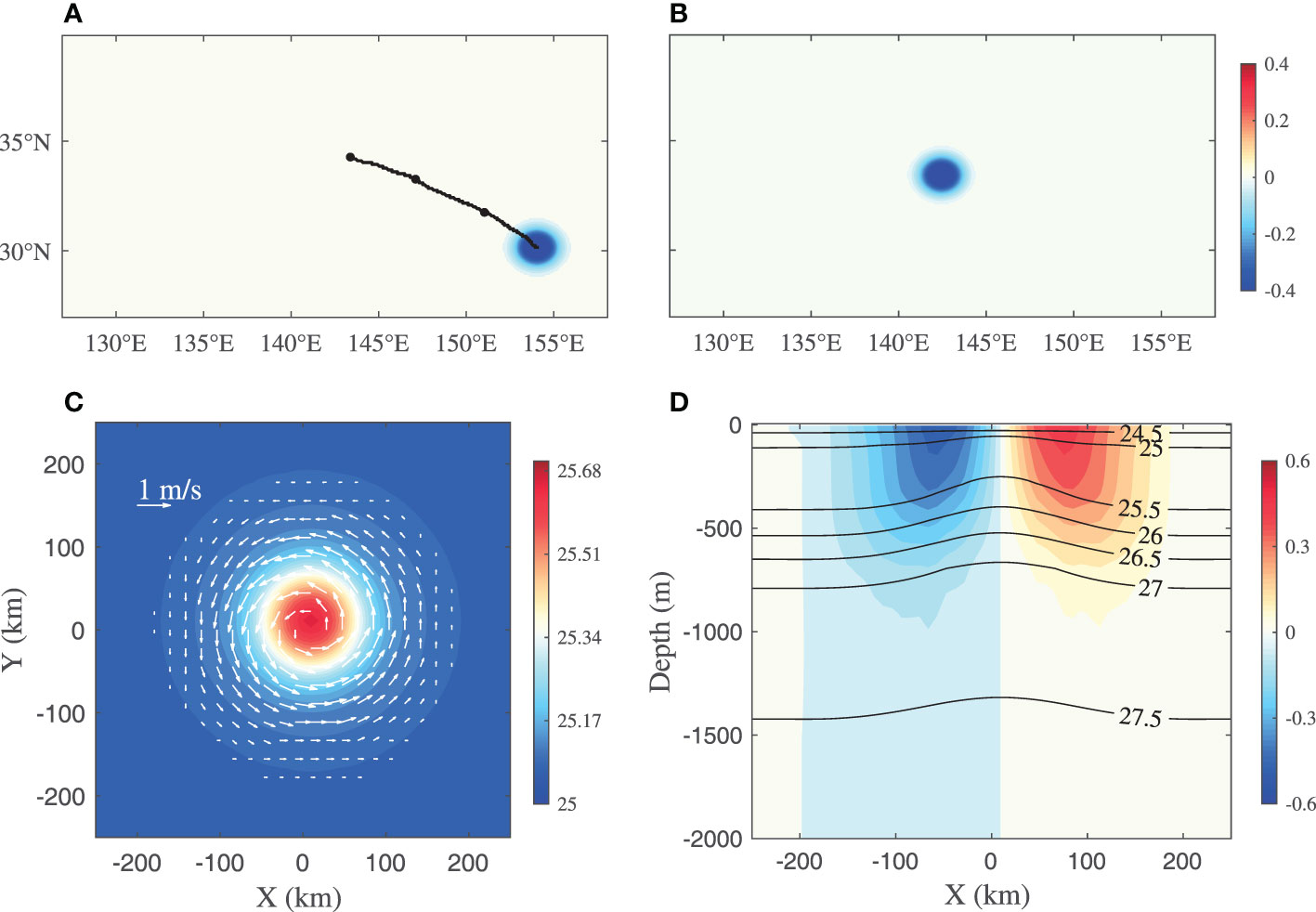
Figure 1 Tracks (black lines) of the idealized eddies on the (A) β-plane and (B) f-plane and the initial conditions of the idealized eddy, including (C) the potential density (shading) and horizontal velocity (vectors) at a depth of 200 m and (D) the vertical distribution of meridional velocity across the center of the eddy in the zonal direction. The color in (A) denotes the sea surface height.

To construct the initial condition of an idealized eddy, we choose a strong isolated cold eddy near the Kuroshio extension from OFES outputs (an example eddy described in section 2.2). First, the polar projection method is used by averaging the potential density (ρ) and sea surface height of the eddy on the same radius to obtain their mean values with respect to each radius and depth to reconstruct an isolated symmetric cold eddy (Figure 1). The zonal and meridional velocities (u, v) are obtained by the geostrophic balance. Initially, w is set to zero, and the background ρ is set to the same value as that on the eddy edge (horizontally uniform). The initial settings of the two experiments are identical, except that in one experiment, f is set to a constant value at 30°N, where the eddy center is. The analysis period is set from day 20 to day 200 to exclude the initial adjustment period and the later period when the eddies become too weak.

Due to energy dissipation, the strengths of the idealized eddies decrease quasi-linearly with time. To eliminate the influence of eddy strength weakening, the w rescaled by eddy strength (V), i.e.,$w_r=w·\frac{V_0}{V}$, will be used in the following analysis, where V is the spatial average of rotation speed ($\sqrt{u^2+v^2}$) on the upper 200 m within the eddy radius and V₀ is the V at the beginning day of analysis.

Isolated eddies from OFES outputs

As is well known, isolated mesoscale eddies are present all over the oceans, such as the Agulhas rings in the South Atlantic Ocean and the strong eddies shedding from the meanders of the Gulf Stream and Kuroshio. In section 3.3, we also examine some isolated eddies from the outputs of OFES to compare the w patterns. OFES is a global eddy-resolving model with a horizontal resolution of 1/10° and 54 vertical levels, and it spans from January 1980 to December 2016. The vertical grid spacing varies from 5 m at the surface to 330 m at a maximum depth of 6065 m. The OFES outputs used here are 3-day snapshots, including ρ, u, v, and w. This widely used dataset (e.g., Sasaki et al., 2008; Masumoto, 2010; Melnichenko et al., 2010) can capture ocean circulations and mesoscale eddies reasonably well.

Two examples of isolated cold/warm eddies in different locations are selected. A warm eddy originating from Cape Agulhas (AWE, hereafter; left panel in Figure 2) is chosen, which has a typical lifetime longer than 2 years and crosses the entire South Atlantic Ocean basin. The analysis period for this eddy was set from January 1, 2016, to October 30, 2016 (303 days), to ensure that the eddy was largely stable and symmetric. Another chosen eddy is a cold eddy near the Kuroshio Extension (KECE, hereafter; right panel in Figure 2). Its lifetime was from May 3, 2012, to September 3, 2012. For the same reason, its analysis period was set from May 18, 2012, to August 25, 2012. Both eddies show obvious westward propagation characteristics (Figure 2A) and are relatively stable during the chosen period. Their maximum rotation speeds are greater than 0.6 m/s, and the density contours and horizontal velocity vectors are all nearly symmetric (Figures 2B–C).

FIGURE 2

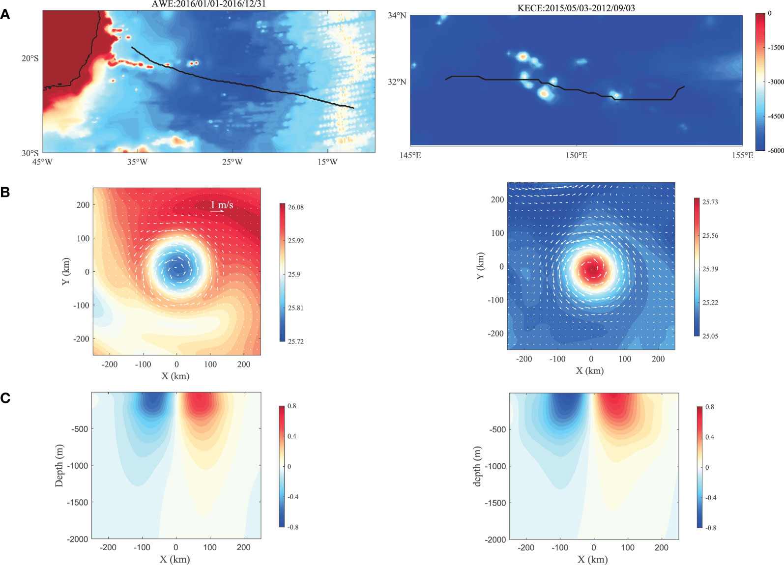
Figure 2 (A) Tracks (black lines) of the Agulhas warm eddy (AWE, left panel) and Kuroshio extension cold eddy (KECE, right panel), and time-mean (B) potential density (shading) and horizontal velocity (vectors) at the depth of 200 m, and (C) vertical distribution of meridional velocity across the center of the AWE (left panel) and KECE (right panel) in the zonal direction. The color in (A) denotes bathymetry.

Eddy detection and tracking method

The eddy detection and tracking method used in this study is the same as that used by Dong et al. (Dong et al., 2011). The eddy center is defined as the point of the velocity minimum. All analyses in the following sections are performed within a square moving with the target eddies. The square is set by positioning the eddy center at its center all the time, with a side length of 500 km. The boundary of the eddy is defined as the maximum closed stream function around the eddy center. The eddy radius is the average distance from each point on the eddy boundary to the eddy center.

Index of w-dipole

To quantify the w-dipole strength, we defined an index of w-dipole (Δw) as the difference of the $\overline{w}$ between the east and west halves within the eddy radius, i.e., $\Delta \overline{w}={\overline{w}}_w-{\overline{w}}_e$, where the overbar denotes the depth-averaged value on the upper 2000 m, and the subscripts w and e represent the west and east half of the eddy, respectively.

QG w-thinking and an “eddy β-spiral” mechanism

Vertical motions of oceanic mesoscale eddies can be delineated through the so-called QG w-thinking using the w-equation (Holton and Hakim, 2013); the latter is also referred to as the Omega equation, as it was often expressed in p coordinates in traditional meteorological applications and in the earlier editions of Holton’s textbook. The w-equation in Cartesian coordinates on the β-plane can be written as

$\begin{array}{ll}\begin{array}{c}{f}^2\frac{{\partial }^{2}w}{\partial z^2}+{\nabla }_h^2\left(N^{2}w\right)=F\end{array}& (1)\end{array}$

 where $N^2=-\frac{g}{\rho }\frac{\partial \rho }{\partial z}$ is the squared Brunt-Väisälä frequency, g is the gravitational acceleration and ${\nabla }_h^2=\left(\frac{{\partial }^2}{\partial x^2}+\frac{{\partial }^2}{\partial y^2}\right)$ is the horizontal Laplacian operator. Omitting the external forcings and mixing, F can be expressed as

$\begin{array}{ll}\begin{array}{c}F=f\frac{\partial }{\partial z}\left[\stackrel{\rightharpoonup }{V}·{\nabla }_h\zeta \right]-\frac{g}{{\rho }_0}{\nabla }_h^2\left(\stackrel{\rightharpoonup }{V}·{\nabla }_h\rho \right)+f\beta \frac{\partial v}{\partial z}\end{array}& (2)\end{array}$

where$\stackrel{\rightharpoonup }{V}·{\nabla }_h=\left(u\frac{\partial }{\partial x}+v\frac{\partial }{\partial y}\right)$ is the horizontal gradient operator, and $\zeta =\frac{\partial v}{\partial x}-\frac{\partial u}{\partial y}$ is the relative vorticity. The first 2 terms on the right−hand side (rhs) of Eq. (2) may be rewritten in the popular form of the Q−vector (e.g., Giordani et al., 2006; Holton and Hakim, 2013; Qiu et al., 2020).

For the gyre-scale circulation, due to the planetary scale, the first two terms on the rhs of Eq. (2) and the horizontal Laplacian operator part on the left of Eq. (1) are negligible, and this w-equation (1) will be reduced to $f^2\frac{{\partial }^{2}w}{\partial z^2}=f\beta \frac{\partial v}{\partial z}$, which is the same except with a removable vertical differentiation for determination of the weak and planetary-scale vertical motion of the “β-spiral”, as suggested by Stommel and Schott (Stommel and Schott, 1977), who directly used the vorticity balance equation $f\frac{\partial w}{\partial z}=\beta v$ instead of the w-equation (1). It should be mentioned, however, the vorticity balance $f\frac{\partial w}{\partial z}=\beta v$ is not valid for isolated but moving near symmetric eddy as the vorticity tendency cannot be ignored as it was for quasi-steady planetary-scale circulation in Stommel and Schott (1977). For eddy-scale vertical motions, the first two terms on the rhs of Eq. (2) normally dominate, the third term is the “β-term” and is generally regarded to be smaller and thus ignored (e.g., Allen and Smeed, 1996; Allen et al., 2001; Qiu et al., 2020), and an f-plane approximation is often used (e.g., Nardelli, 2013; Pidcock et al., 2013).

Here, we propose to consider a “β-spiral” for an isolated symmetric eddy. In this case, the contours of ρ and ζ are symmetric and parallel so that the first two terms on the rhs of Eq. (2) are nearly zero because $\stackrel{\rightharpoonup }{V}·{\nabla }_h\rho \approx 0,\stackrel{\rightharpoonup }{V}·{\nabla }_h\zeta \approx 0$. As a result, the w-equation (1) is greatly simplified into the following form:

$\begin{array}{ll}\begin{array}{c}{f}^2\frac{{\partial }^{2}w}{\partial z^2}+ {\nabla }_h^2\left(N^{2}w\right)=f\beta \frac{\partial v}{\partial z} \end{array}& (3)\end{array}$

Because the horizontal Laplacian operator only quantitatively affects the strength and pattern, we thus term the β-effect induced eddy vertical motion as an “eddy β-spiral” mechanism, which is a true extension for the planetary-scale “β-spiral” (Stommel and Schott, 1977) mechanism. This simple “eddy β-spiral” mechanism predicts that because an isolated mesoscale eddy always has an east-west dipole pattern in its meridional velocity, its vertical motion will also be dominated by an east-west dipole pattern with its strength proportional to eddy meridional velocity. Moreover, this w-dipole has a notable deep ocean vertical penetration to the ocean bottom as the “β-spiral” does. We will show supporting evidence with examples of numerical experiments and eddy-resolving model outputs in the next sections.

In the following analysis, using the outputs of the contrasting experiments and OFES, the vertical motions in isolated eddies will be reconstructed by solving Eq. (1) with the same method as that in Qiu et al. (2020). To this end, the model outputs were first used to calculate the terms in Eq. (2). After that, by Fourier transformation, w (x, y, z) and F (x, y, z) become $\widehat{w}$ (k_x, k_y, z) and $\widehat{F}$(k_x, k_y, z). Consequently, for each pair of horizontal wavenumbers k_x and k_y, $\widehat{w}$ (k_x, k_y, z) is solved numerically according to discretized Eq. (1) using centered differencing in the z direction and the boundary conditions. Once $\widehat{w}$(k_x, k_y, z) is solved, w (x, y, z) is obtained via inverse Fourier transformation. The boundary conditions in the idealized experiments are set as w=0 at the  z=0 and bottoms, and those for OFES outputs are set as w=0 at  z=0 and $\frac{\partial w}{\partial z}=0$ at z=2000  m to avoid the influence of topography. Notably, the contributions to w from each term in F can be easily evaluated separately using the diagnostic w-equation (1).

It is notable that, the sub-mesoscale processes play important roles in vertical transport in the ocean. In the present study, we only considered the isolated mesoscale eddies and used the QG framework in this study. Therefore, the effects of sub-mesoscale processes on w cannot be fully included in the simulation. However, the QG-w dynamics that we have adopted are shown capable of capturing a broadscale of vertical motion, whereas ageostrophic and other processes tend to be important for fine spatial or short temporal scales of vertical motion, as demonstrated in Qiu et al. (2019).

Result

Evidence of the w-dipole from idealized eddy experiments

Relative to horizontal velocity, very small vertical motions in eddies cannot be directly measured instrumentally and can only be inferred diagnostically or simulated consistently in eddy-resolving models. To test the “eddy β-spiral” mechanism, we design a pair of contrasting numerical experiments of the idealized isolated eddy on the β-plane and the f-plane, as briefly described in section 2.1.

After a 20-day quick geostrophic adjustment, the idealized cold eddy on the β-plane is found to propagate northwestward, and its time mean surface ρ and horizontal velocity are all in a stable and nearly symmetric round shape (the left column in Figure 3 and Video S1). Simultaneously, its eddy-induced vertical motion is indeed dominated by a pronounced and stable east-west dipole pattern (the right column in Figure 3 and Video S2). It can also be seen that the w-dipole pattern is more significant at the beginning days when the horizontal velocity is stronger. Then, it gradually becomes weaker with the slowing of the rotational speed of the eddy (Figure 3). In contrast, the identical eddy on the f-plane is found to remain stationary all the time (the left column in Figure 4 and Video S3). However, the corresponding vertical motion induced by the eddy on the f-plane looks very weak and has no stable pattern at all (the right column in Figure 4 and Video S4). The magnitude of the time mean $\overline{w_r}$ induced by the eddy on the β-plane reaches 4.6×10^-5 m/s (Figure 5A), approximately one order of magnitude larger than that of the eddy on the f-plane (figure not shown). Since the only difference between these two experiments is the β-effect, this contrasting pair of numerical experiments verified not only the existence of a w-dipole in an isolated eddy as predicted by our “eddy β-spiral” mechanism but also the disappearance of the w-dipole when the β-effect is removed for a nearly symmetric isolated eddy. Yang et al. (2020) conducted a numerical simulation of an isolated warm eddy on the β-plane to study eddy tilting. However, in their result, the eddy w at model day 10 exhibited a dipole pattern in the NW-SE direction, rather than east-west, if it was purely from the β-effect. This difference may be due to the instability of the eddy, which causes eddy structure variations at that time, as the time-averaged w-dipole should be east-west oriented according to our “eddy β-spiral” mechanism.

FIGURE 3

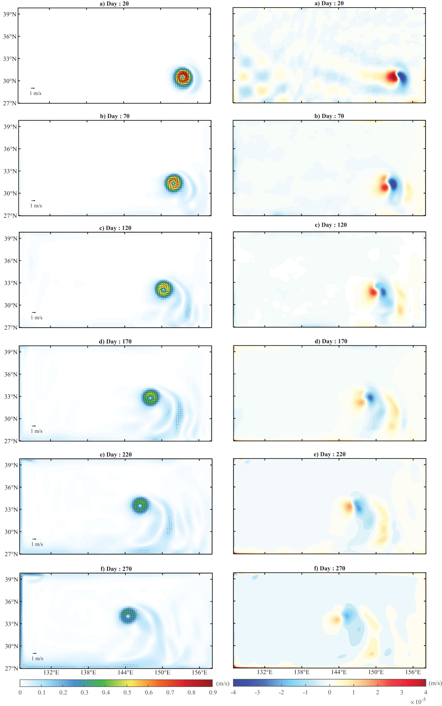
Figure 3 Time evolutions of the horizontal velocity (left column, vectors) and vertical velocity (right column, shading) of the idealized eddy on the β-plane at days 20, 70, 120, 170, 220, and 270. The shading in the left column presents the magnitude of horizontal velocity.

FIGURE 4

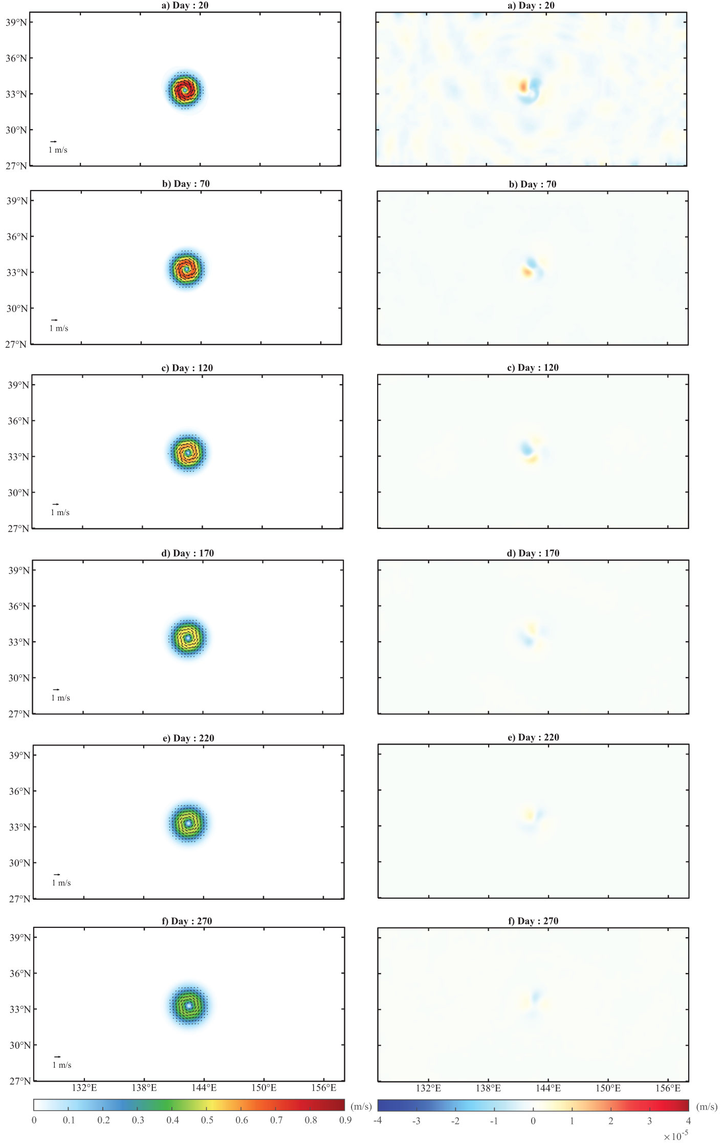
Figure 4 Same as Figure 3 except for the idealized eddy on the f-plane.

FIGURE 5

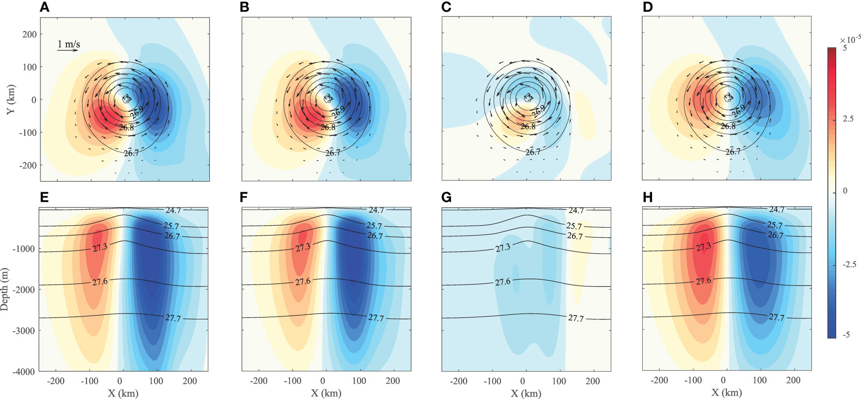
Figure 5 Time-mean depth-averaged (0~2000 m) w in the idealized eddy on the β-plane (upper row) obtained from the (A) ROMS outputs, (B) w-equation with all terms, (C) w-equation without the β-term, and (D) w-equation with the β-term only (shading), superimposed by the time mean ρ (contours) and horizontal velocity (vectors) on the surface, and corresponding vertical profiles of w across the eddy centers in the zonal direction lower row, (E–H), superimposed by the time mean ρ (contours).

Moreover, as described in section 3, we may use the w-equation (1) to further diagnose the eddy w in this quantitation. The total solution from the w-equation (1) considering the β-term almost fully captures the eddy-induced w on the β-plane, with the former being only 5% weaker than the latter (Figure 5B). However, omitting the β-term (Figure 5C), the magnitude of the w solution is much smaller (<1×10^-5 m/s), and this part is due to the weak asymmetry that remains in the time mean eddy structure. Similar w solutions with comparable magnitudes were also obtained in other studies (Barceló-Llull et al., 2017; Mason et al., 2017) with the β-term being omitted from the w-equation (1). In contrast, the contribution to w from the β-term (Figure 5D) shows a significant dipole pattern, with a magnitude very close to that of the model result (Figure 5A). Comparing the magnitude of w fields in Figure 5, the w-dipole induced by the “eddy β-spiral” accounts for 86% of the total w, clearly demonstrating the dominance of the “eddy β-spiral” mechanism in a nearly symmetric isolated eddy.

According to the “eddy β-spiral” mechanism, the w in the eddy is supposed to be significantly amplified with depth due to the vertically cumulative effect of the β-spiral. The east-west vertical cross-section of w in the idealized eddy on the β-plane (Figure 5E) confirmed this conjecture. This w-dipole pattern is seen to be very weak in the upper layer but increases dramatically with depth. Its maximum reaches 5.4×10^-5 m/s at approximately h = 1000 m, one order of magnitude greater than that at h = 50 m. Meanwhile, the corresponding v field decreases drastically with depth. The maximum v at h = 1000 m is 0.07 m/s, which is only 9% of its surface value. This result implies that the w-dipole is much stronger in the deep layer where the eddy horizontal motion becomes much weaker. This relatively strong w beneath the main eddy body may exert a considerable impact on deep ocean mixing and mass transport. Based on the moorings of the Scientific Observation Network of the Chinese Academy of Sciences in the western Pacific, Ma et al. (2019) observed a series of intensified temperature variabilities in a deep channel (~4000 m) at the Pacific Yap‐Mariana Junction. They suggested that these deep ocean variabilities are likely generated by energetic surface eddies moving across the rough topography. This observation may be possible evidence of the impact of the eddy w-dipole on the deep layer, which needs further verification.

The vertical profile of w determined by the w-equation (1) with all terms (Figure 5F) is nearly identical to that of the simulated w. Consistent with its horizontal distribution, the vertical cross-section of w is also dominated by the β-term, which accounts for 84% of the total w (Figures 5G, H). Notably, the eddy w-dipole does not reach its maximum at the bottom because of the boundary condition w = 0 at the flat bottom.

In brief, the contrasting idealized eddy experiments on the β-plane and the f-plane verified that the “eddy β-spiral” is the dominant mechanism for the formation of w-dipole patterns in nearly symmetric isolated eddies. The β-term must be considered in the w-equation (1) for the study of vertical motions in mesoscale eddies.

Evidence from OFES outputs

Similar w-dipoles due to the “eddy β-spiral” can also be found in isolated eddies simulated by the other eddy-resolving models. Here, two examples of isolated eddies from the OFES outputs described in section 2.2 are analyzed to confirm the existence of the w-dipole patterns in isolated eddies. Consistent with the situation in the idealized eddy on the β-plane, the time mean $\overline{w}$ in both eddies has significant east-west dipole patterns (Figures 6A and 7A), with their maximum magnitudes reaching 6.4×10^-5 m/s and 7.6×10^-5 m/s in the AWE and KECE cases, respectively. There is an upwelling/downwelling zone in the eastern part of the warm/cold eddy. Opposite polarities of the w-dipole of cold/warm type are simply due to their opposite polarities of v dipoles, as can be inferred from the “eddy β-spiral” w-equation (3).

FIGURE 6

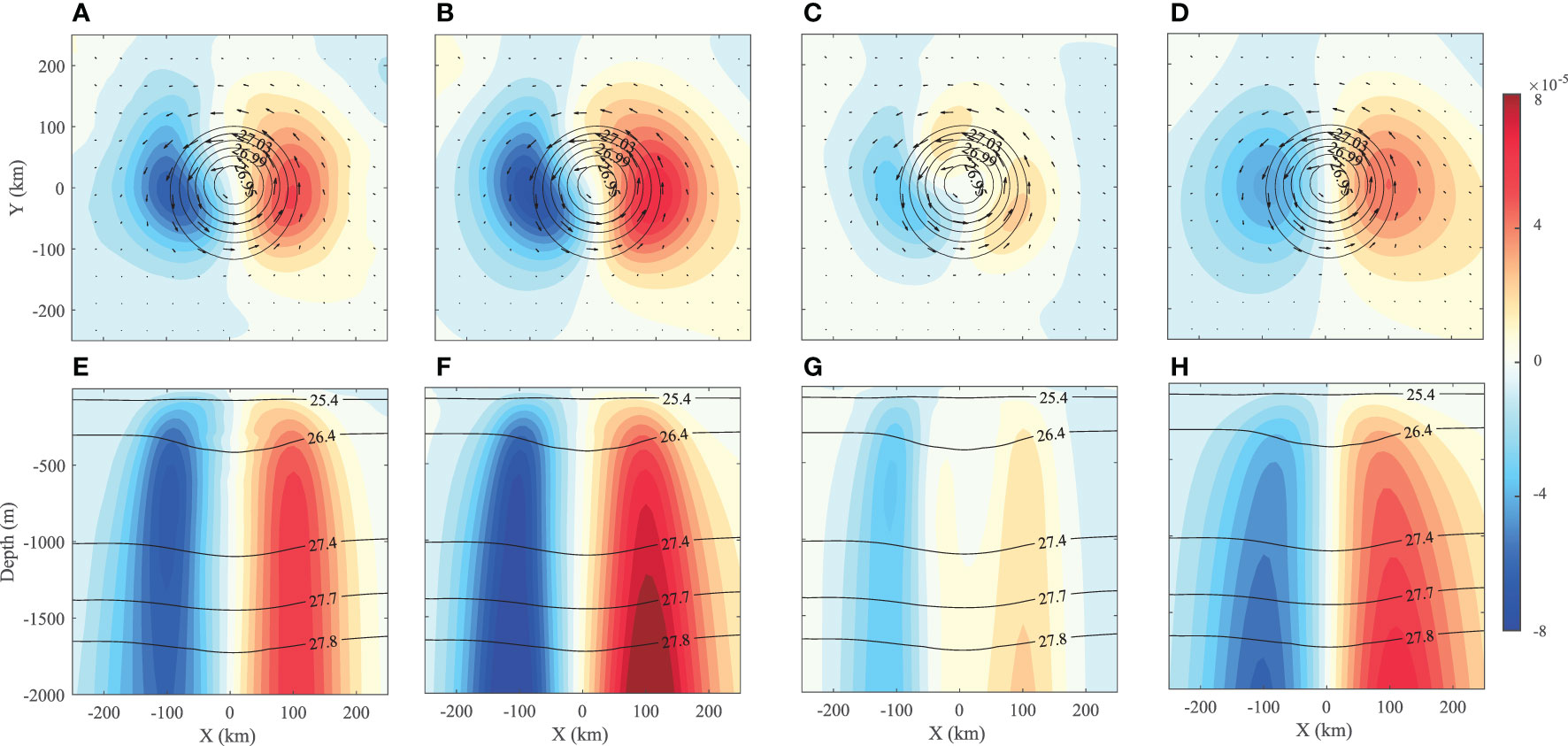
Figure 6 Same as Figure 5 except for the case of the Agulhas warm eddy (AWE).

FIGURE 7

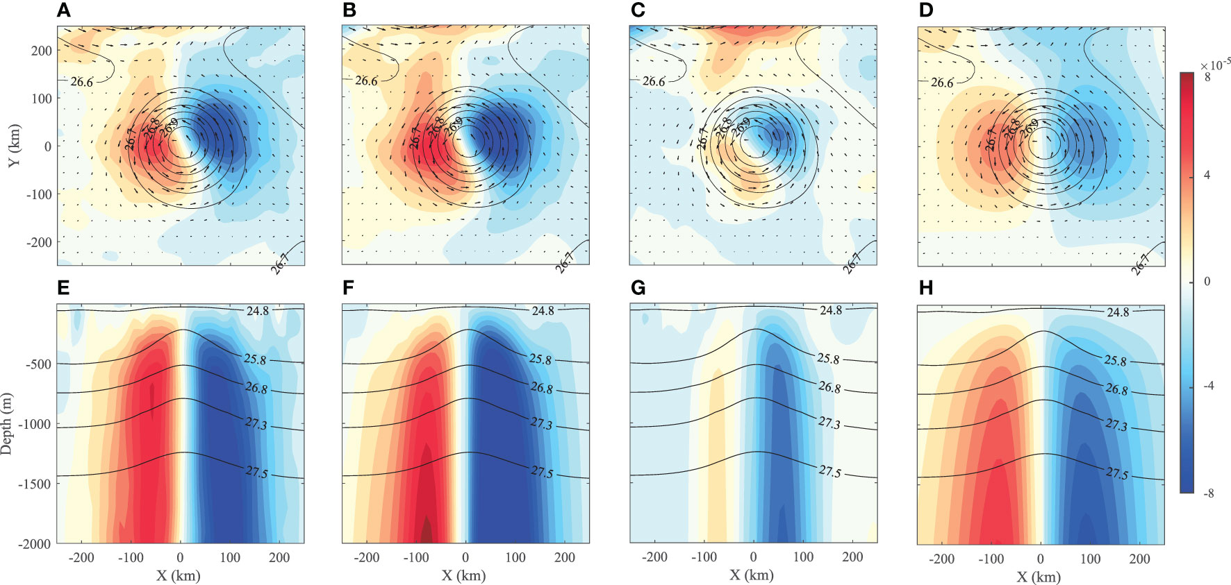
Figure 7 Same as Figure 5 except for the case of the Kuroshio extension cold eddy (KECE).

The solutions of the w-equation (1) considering all terms in F (Figures 6B and 7B) show nearly identical dipole patterns as OFES outputs, with the former being approximately 10% stronger than the latter. A part of this difference is due to the artificial bottom boundary condition, $\frac{\partial w}{\partial z}=0$ at z = 2000 m, which only alters the solution above 2000 m in a minor manner and is set to avoid the complications associated with complex bottom topography. Meanwhile, w solutions omitting the β-term (Figures 6C and 7C) are much weaker than the w from OFES outputs, and these remaining parts due to the weak asymmetry in the mean eddy structure account for only approximately 1/4 of the total w. In contrast, solutions considering the β-term alone (Figures 6D and 7D) showed significant w-dipole patterns. Comparing the averaged magnitudes of w in Figures 6 and 7, the w-dipoles induced by the “eddy β-spiral” in the AWE and KECE are found to account for 72% and 74% of the total w, respectively, again confirming that the “eddy β-spiral” dominates the w-dipoles in nearly symmetric isolated eddies.

Consistent with that of the idealized simulation on the β-plane, the w-dipoles in both eddies appear very weak near the surface but increase dramatically with depth (Figures 6E and 7E). Their maxima at h = 2000 m reach 6.8×10^-5 m/s and 9.7×10^-5 m/s in AWE and KECE, respectively, which are one order greater than those at h = 50 m. The vertical profiles of the solutions by the w-equation (1) (Figures 6G, H and 7G, H) are quite similar to those from the idealized simulation on the β-plane. Corresponding to their horizontal distributions, vertical profiles of the w solutions due to the β-term alone (Figures 6H and 7H) present significant dipole patterns, which are 3 times stronger than those induced by other terms in F (Figures 6C and 7C). In conclusion, these two examples further demonstrate the dominance of w-dipoles in isolated eddies, which is induced by the β-effect and can be well explained by the “eddy β-spiral” mechanism.

The w-dipole index

To develop a simple index to quantify the w-dipole in eddies, we introduced a w-dipole index in section 2.4. For example, the time mean w-dipole index from the model outputs (Δw_model ) of the idealized eddy on the β-plane is 2.7×10^-5 m/s, 240 times stronger than that on the f-plane (1.1×10^-7 m/s), which provides us with a quantitative measure for the dominance of w-dipoles by the “eddy β-spiral” (Figure 8A) in the pair of idealized simulations.

FIGURE 8

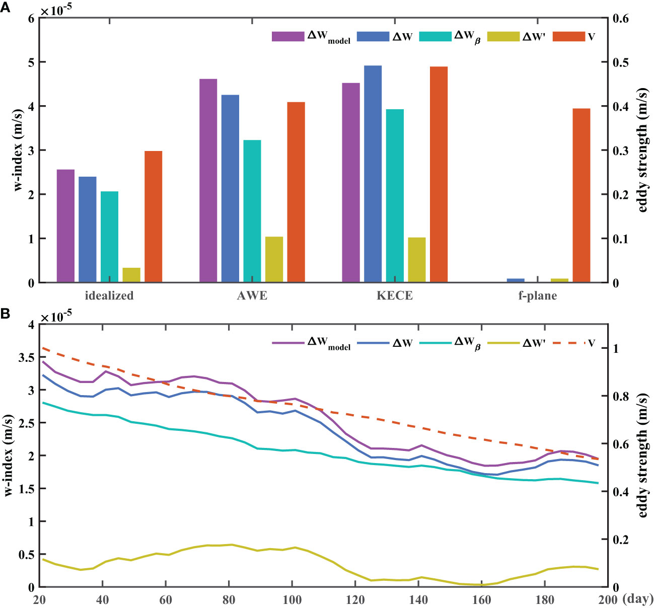
Figure 8 (A) Bar diagram of the time mean w-dipole indices obtained from model outputs (Δw_model, purple bars), w-equation with all terms (Δw, blue bars), w-equation with the β-term only (Δw_β,  green bars) and w-equation without the β-term (Δw",  yellow bars) for the idealized eddy on the β-plane (β-plane), the Agulhas warm eddy (AWE), the Kuroshio extension cold eddy (KECE) and the idealized eddy on the f-plane (f-plane), respectively. Red bars represent the corresponding eddy strength (V). (B) Temporal variation in the w-dipole indices and the corresponding eddy strength (V) of the idealized eddy on the β-plane.

The time mean w-dipole indices from the w-equation (1) solutions with all terms (Δw) are found to be very close to Δw_model . The relative errors ($\frac{\Delta w_{model}-\Delta w}{\Delta w_{model}}$) are 6.4%, 8.1% and -8.7% in the idealized eddy on the β-plane, KECE and AWE, respectively, confirming the accuracy of w reconstructed by the w-equation (1). As expected, the time mean w-dipole indices from the solutions considering the β-term alone (Δw_β ) account for 86.2%, 79.9% and 74.8% of Δw in the idealized eddy on the β-plane, KECE and AWE, respectively, demonstrating the dominance of the “eddy β-spiral” effect on w-dipoles again. Meanwhile, the contribution of the first two terms of the rhs of Eq. (2) to the indexes (Δw ) account for the remaining 15%~25%, indicating that the weak asymmetry in the eddy will also produce nonnegligible contributions to the w-dipole, which has been investigated in previous studies (e.g., Nardelli, 2013; Pidcock et al., 2013; Barceló-Llull et al., 2017; Mason et al., 2017). In a symmetric eddy, the w-dipole will be absolutely dominant, as the “eddy β-spiral” mechanism predicts. The larger the asymmetry is, the lower the β-effect dominance.

The comparisons of w-dipole indices and eddy strengths of different eddies from the model outputs and w-equation (1) solutions indicate that the greater the eddy strength is, the stronger the w-dipole (Figure 8A). In particular, in terms of the solution of the w-equation that considers the β-term alone (Eq.3), the corresponding w-dipole index, Δw_β , is expected to increase linearly with the eddy strength (Figure 8B). Meanwhile, there is a significant temporal variation in the w-dipole with the evolution of the eddy (Figure 8B), which will be discussed separately in another paper.

In the classic “β-spiral” theory proposed by Stommel and Schott (1977), a greatly simplified vorticity equation, $f\frac{\partial w}{\partial z}=\beta v$, is used instead of the more accurate w-equation for the gyre−scale circulation. However, it is not applicable for the mesoscale processes, where the scales of other terms in the w-equation are likely comparable to that of βv . In the case of isolated eddy, the w-equation (1) is simplified into Eq. (3). Thus, the main difference from the β-spiral vorticity equation is the Laplacian term, ${\nabla }_h^2\left(N^{2}w\right),$although our use of w-equation also allows applying proper surface and bottom boundary condition for w, the horizonal Laplacian term tends to inflate the horizonal patterns of v and reduce the strength of the eddy w-dipole due to β-effect. To quantitative evaluation of the contribution of the Laplacian term, we recalculated the w of the idealized eddy by setting N²=0  in the w-equation. The difference between the solution with and without this term is as expected (not shown). In fact, the larger the eddy size than the Rossby radius deformation, the smaller this effect is and the fuller of β-spiral effect as noted by Stommel and Schott (1977). The smaller the eddy size, the stronger reduction on the β-spiral effect will be.

Conclusions and discussions

This study revealed that there is a robust east-west oriented w-dipole in an isolated and nearly symmetric mesoscale eddy induced by the β-effect. In particular, it can extend to the very deep ocean. This eddy w-dipole pattern can be understood simply by the “eddy β-spiral” mechanism, which is approximately described by the simplified w-equation (3). Therefore, the β-term should not be ignored in the w-equation (1) during the study of eddy vertical motions.

The significance of this study is threefold. First, it suggests that the isolated warm (cold) eddies have an upwelling (downwelling) center on their western side and a downwelling (upwelling) center on their eastern side. Second, the robust w-dipoles in isolated eddies do not conform to the conventional concept of monopole downwelling (upwelling) in cold (warm) eddies. In particular, this result suggests that warm eddies may also pump nutrients from the subsurface to the euphotic layer, which requires further observational validation. Third, the w-dipoles are found to reach significantly deep into the ocean, which may have considerable impacts on deep ocean mixing and vertical mass transport. Further modeling studies of the impacts of deep ocean vertical motion associated with isolated eddies in the presence of weak background diffusion will be reported in forthcoming papers. In addition, this study only demonstrated that the w-dipole induced by the “eddy β-spiral” is dominant on the condition that the eddy is isolated and nearly round. It is likely to be overpowered by other processes for eddies under other conditions. The importance of the “eddy β-spiral” in frontal eddies or eddies with strong deformation also needs to be further evaluated.

Data availability statement

The raw data supporting the conclusions of this article will be made available by the authors, without undue reservation.

Author contributions

YH contributed to the paper writing and data analysis. F-FJ and SG led the preparation of the manuscript with contribution from all authors. F-FJ proposed the eddy β-spiral mechanism and contributed to the paper writing. SG proposed and conceived the study and contributed to the paper writing. JZ conducted the numerical experiment of idealized eddies. KL and SG contribute to the numerical solutions of w-equation. TQ and FW contributed to the discussion and paper writing. All authors contributed to the article and approved the submitted version.

Funding

This study was supported by the Marine S&T Fund of Shandong Province for Pilot National Laboratory for Marine Science and Technology (Qingdao) (No. 2022QNLM010301-4) and the National Natural Science Foundation of China through grants 41676009. F-FJ was supported by the U.S. National Science Foundation (AGS‐1813611 and AGS-2219257) and Department of Energy (DESC0005110).

Acknowledgments

The OFES simulation was conducted on the Earth Simulator under the support of JAMSTEC.

Conflict of interest

The authors declare that the research was conducted in the absence of any commercial or financial relationships that could be construed as a potential conflict of interest.

Publisher’s note

All claims expressed in this article are solely those of the authors and do not necessarily represent those of their affiliated organizations, or those of the publisher, the editors and the reviewers. Any product that may be evaluated in this article, or claim that may be made by its manufacturer, is not guaranteed or endorsed by the publisher.

Supplementary material

The Supplementary Material for this article can be found online at: https://www.frontiersin.org/articles/10.3389/fmars.2022.1036783/full#supplementary-material

References

Allen J. T., Smeed D. A. (1996). Potential vorticity and vertical velocity at the Iceland-færœs front. J. Phys. Oceanogr. 26, 2611–2634. doi: 10.1175/1520-0485(1996)026<2611:PVAVVA>2.0.CO;2

CrossRef Full Text | Google Scholar

Allen J. T., Smeed D. A., Nurser A. J. G., Zhang J. W., Rixen M. (2001). Diagnosis of vertical velocities with the QG omega equation: An examination of the errors due to sampling strategy. Deep. Res. Part I Oceanogr. Res. Pap. 48, 315–346. doi: 10.1016/S0967-0637(00)00035-2

CrossRef Full Text | Google Scholar

Alpine J. E., Hobday A. J. (2007). Area requirements and pelagic protected areas: Is size an impediment to implementation? Mar. Freshw. Res. 58, 558–569. doi: 10.1071/MF06214

CrossRef Full Text | Google Scholar

Barceló-Llull B., Pallàs-Sanz E., Sangrà P., Martínez-Marrero A., Estrada-Allis S. N., Arístegui J. (2017). Ageostrophic secondary circulation in a subtropical intrathermocline eddy. J. Phys. Oceanogr. 47, 1107–1123. doi: 10.1175/JPO-D-16-0235.1

CrossRef Full Text | Google Scholar

Brannigan L. (2016). Intense submesoscale upwelling in anticyclonic eddies. Geophys. Res. Lett. 43, 3360–3369. doi: 10.1002/2016GL067926

CrossRef Full Text | Google Scholar

Chelton D. (2013). Ocean-atmosphere coupling: Mesoscale eddy effects. Nat. Geosci. 6, 594–595. doi: 10.1038/ngeo1906

CrossRef Full Text | Google Scholar

Chelton D. B., Gaube P., Schlax M. G., Early J. J., Samelson R. M. (2011). The influence of nonlinear mesoscale eddies on near-surface oceanic chlorophyll. Sci. (80-. ). 334, 328–332. doi: 10.1126/science.1208897

CrossRef Full Text | Google Scholar

Chelton D. B., Schlax M. G., Samelson R. M., de Szoeke R. A. (2007). Global observations of large oceanic eddies. Geophys. Res. Lett. 34, 1–5. doi: 10.1029/2007GL030812

CrossRef Full Text | Google Scholar

Cotroneo Y., Aulicino G., Ruiz S., Pascual A., Budillon G., Fusco G., et al. (2016). Glider and satellite high resolution monitoring of a mesoscale eddy in the algerian basin: Effects on the mixed layer depth and biochemistry. J. Mar. Syst. 162, 73–88. doi: 10.1016/j.jmarsys.2015.12.004

CrossRef Full Text | Google Scholar

Dong C. M., Nencioli F., Liu Y., McWilliams J. C. (2011). An automated approach to detect oceanic eddies from satellite remotely sensed Sea surface temperature data. IEEE Geosci. Remote Sens. Lett. 8, 1055–1059. doi: 10.1109/LGRS.2011.2155029

CrossRef Full Text | Google Scholar

Early J. J., Samelson R. M., Chelton D. B. (2011). The evolution and propagation of quasigeostrophic ocean eddies. J. Phys. Oceanogr. 41, 1535–1555. doi: 10.1175/2011JPO4601.1

CrossRef Full Text | Google Scholar

Falkowski P. G., Ziemann D., Kolber Z., Bienfang P. K. (1991). Role of eddy pumping in enhancing primary production in the ocean. Nature 352, 55–58. doi: 10.1038/352055a0

CrossRef Full Text | Google Scholar

Gaube P., Chelton D. B., Samelson R. M., Schlax M. G., O’Neill L. W. (2015). Satellite observations of mesoscale eddy-induced ekman pumping. J. Phys. Oceanogr. 45, 104–132. doi: 10.1175/JPO-D-14-0032.1

CrossRef Full Text | Google Scholar

Giordani H., Prieur L., Caniaux G. (2006). Advanced insights into sources of vertical velocity in the ocean. Ocean Dyn. 56, 513–524. doi: 10.1007/s10236-005-0050-1

CrossRef Full Text | Google Scholar

Holton J. R., Hakim G. J. (2013). An introduction to dynamic meteorology. fifth (Elsevier: Academic Press). doi: 10.1016/B978-0-12-384866-6.00006-4

CrossRef Full Text | Google Scholar

Huang R. X. (Ed.) (2009). “Dynamical foundations,” in Ocean circulation: Wind-driven and thermohaline processes (Cambridge: Cambridge University Press), 63–148. doi: 10.1017/CBO9780511812293.003

CrossRef Full Text | Google Scholar

Klein P., Lapeyre G. (2009). The oceanic vertical pump induced by mesoscale and submesoscale turbulence. Ann. Rev. Mar. Sci. 1, 351–375. doi: 10.1146/annurev.marine.010908.163704

PubMed Abstract | CrossRef Full Text | Google Scholar

Lévy M., Klein P., Treguier A. M. (2001). Impact of sub-mesoscale physics on production and subduction of phytoplankton in an oligotrophic regime. J. Mar. Res. 59, 535–565. doi: 10.1357/002224001762842181

CrossRef Full Text | Google Scholar

Mason E., Pascual A., Gaube P., Ruiz S., Pelegrí J. L., Delepoulle A. (2017). Subregional characterization of mesoscale eddies across the Brazil-malvinas confluence. J. Geophys. Res. Ocean. 122, 3329–3357. doi: 10.1002/2016JC012611

CrossRef Full Text | Google Scholar

Masumoto Y. (2010). Sharing the results of a high-resolution ocean general circulation model under a multi-discipline framework - a review of OFES activities. Ocean Dyn. 60, 633–652. doi: 10.1007/s10236-010-0297-z

CrossRef Full Text | Google Scholar

Ma Q., Wang F., Wang J., Lyu Y. (2019). Intensified deep ocean variability induced by topographic rossby waves at the pacific yap-Mariana junction. J. Geophys. Res. Ocean. 124, 8360–8374. doi: 10.1029/2019JC015490

CrossRef Full Text | Google Scholar

McGillicuddy J. J., Anderson L. A., Doney S. C., Maltrud M. E. (2003). Eddy-driven sources and sinks of nutrients in the upper ocean: Results from a 0.1° resolution model of the north Atlantic. Global Biogeochem. Cycles 17, 1035. doi: 10.1029/2002gb001987

CrossRef Full Text | Google Scholar

McGillicuddy D. J., Robinson A. R., McCarthy J. J. (1995). Coupled physical and biological modelling of the spring bloom in the north Atlantic (II): three dimensional bloom and post-bloom processes. Deep. Res. Part I 42, 1359–1398. doi: 10.1016/0967-0637(95)00035-5

CrossRef Full Text | Google Scholar

McGillicuddy D. J., Robinson A. R., Siegel D. A., Jannasch H. W., Johnson R., Dickey T. D., et al. (1998). Influence of mesoscale eddies on new production in the Sargasso Sea. Nature 394, 263–266. doi: 10.1038/28367

CrossRef Full Text | Google Scholar

McWilliams J. C., Graves L. P., Montgomery M. T. (2003). A formal theory for vortex rossby waves and vortex evolution. Geophys. Astrophys. Fluid Dyn. 97, 275–309. doi: 10.1080/0309192031000108698

CrossRef Full Text | Google Scholar

Melnichenko O. V., Maximenko N. A., Schneider N., Sasaki H. (2010). Quasi-stationary striations in basin-scale oceanic circulation: Vorticity balance from observations and eddy-resolving model. Ocean Dyn. 60, 653–666. doi: 10.1007/s10236-009-0260-z

CrossRef Full Text | Google Scholar

Montgomery M. T., Kallenbach R. J. (1997). A theory for vortex rossby-waves and its application to spiral bands and intensity changes in hurricanes. Q. J. R. Meteorol. Soc 123, 435–465. doi: 10.1256/smsqj.53809

CrossRef Full Text | Google Scholar

Nardelli B. B. (2013). Vortex waves and vertical motion in a mesoscale cyclonic eddy. J. Geophys. Res. Ocean. 118, 5609–5624. doi: 10.1002/jgrc.20345

CrossRef Full Text | Google Scholar

Nemcek N., Ianson D., Tortell P. D. (2008). A high-resolution survey of DMS, CO2, and O2/Ar distributions in productive coastal waters. Global Biogeochem. Cycles 22, GB2009. doi: 10.1029/2006GB002879

CrossRef Full Text | Google Scholar

Oke P. R., Griffin D. A. (2011). The cold-core eddy and strong upwelling off the coast of new south Wales in early 2007. Deep Sea Res. Part II Top. Stud. Oceanogr. 58, 574–591. doi: 10.1016/j.dsr2.2010.06.006

CrossRef Full Text | Google Scholar

Oliver E. C. J., Holbrook N. J. (2014). Extending our understanding of south pacific gyre “spin-up”: Modeling the East Australian current in a future climate. J. Geophys. Res. Ocean. 119, 2788–2805. doi: 10.1002/2013JC009591

CrossRef Full Text | Google Scholar

Pidcock R., Martin A., Allen J., Painter S. C., Smeed D. (2013). The spatial variability of vertical velocity in an Iceland basin eddy dipole. Deep. Res. Part I Oceanogr. Res. Pap. 72, 121–140. doi: 10.1016/j.dsr.2012.10.008

CrossRef Full Text | Google Scholar

Pilo G. S., Oke P. R., Coleman R., Rykova T., Ridgway K. (2018). Patterns of vertical velocity induced by eddy distortion in an ocean model. J. Geophys. Res. Ocean. 123, 2274–2292. doi: 10.1002/2017JC013298

CrossRef Full Text | Google Scholar

Qiu B., Chen S., Klein P., Torres H., Wang J., Fu L. L., et al. (2019). Reconstructing upper ocean vertical velocity field from sea surface height in the presence of unbalanced motion. J. Phys. Oceanogr. 49, 55–79. doi: 10.1175/JPO-D-19-0172.1

CrossRef Full Text | Google Scholar

Qiu B., Chen S., Klein P., Torres H., Wang J., Fu L. L., et al. (2020). Reconstructing upper-ocean vertical velocity field from Sea surface height in the presence of unbalanced motion. J. Phys. Oceanogr. 50, 55–79. doi: 10.1175/JPO-D-19-0172.1

CrossRef Full Text | Google Scholar

Qiu Bo, Xin Huang R. (1995). Ventilation of the north Atlantic and north pacific: subduction versus obduction. J. Phys. Oceanogr. 25, 2374–2390. doi: 10.1175/1520-0485(1995)025<2374:votnaa>2.0.co;2

CrossRef Full Text | Google Scholar

Qu T., Gao S., Fukumori I., Fine R. A., Lindstrom E. J. (2008). Subduction of south pacific waters. Geophys. Res. Lett. 35, L02610. doi: 10.1029/2007GL032605

CrossRef Full Text | Google Scholar

Sasaki H., Nonaka M., Masumoto Y., Sasai Y., Uehara H., Sakuma H. (2008). “An eddy-resolving hindcast simulation of the quasiglobal ocean from 1950 to 2003 on the earth simulator,” in High resolution numerical modelling of the atmosphere and ocean (New York, NY: Springer New York), 157–185. doi: 10.1007/978-0-387-49791-4_10

CrossRef Full Text | Google Scholar

Shchepetkin A. F., McWilliams J. C. (2005). The regional oceanic modeling system (ROMS): A split-explicit, free-surface, topography-following-coordinate oceanic model. Ocean Model. 9, 347–404. doi: 10.1016/j.ocemod.2004.08.002

CrossRef Full Text | Google Scholar

Siegel D. A., Peterson P., McGillicuddy D. J., Maritorena S., Nelson N. B. (2011). Bio-optical footprints created by mesoscale eddies in the Sargasso Sea. Geophys. Res. Lett. 38, L13608. doi: 10.1029/2011GL047660

CrossRef Full Text | Google Scholar

Stommel H., Schott F. (1977). The beta spiral and the determination of the absolute velocity field from hydrographic station data. Deep Sea Res. 24, 325–329. doi: 10.1016/0146-6291(77)93000-4

CrossRef Full Text | Google Scholar

Sun B., Liu C., Wang F. (2019). Global meridional eddy heat transport inferred from argo and altimetry observations. Sci. Rep. 9, 1–10. doi: 10.1038/s41598-018-38069-2

PubMed Abstract | CrossRef Full Text | Google Scholar

Sun B., Liu C., Wang F. (2020). Eddy induced SST variation and heat transport in the western north pacific ocean. J. Oceanol. Limnol. 38, 1–15. doi: 10.1007/s00343-019-8255-1

CrossRef Full Text | Google Scholar

Tomczak M., Godfrey J. (2003). Regional oceanography: An introduction. 2nd (New Delhi, India: Daya Publishing House).

Google Scholar

Viúdez Á., Dritschel D. G. (2003). Vertical velocity in mesoscale geophysical flows. J. Fluid Mech. 483, 199–223. doi: 10.1017/S0022112003004191

CrossRef Full Text | Google Scholar

Wunsch C. (1999). Where do ocean eddy heat fluxes matter? J. Geophys. Res. Ocean. 104, 13235–13249. doi: 10.1029/1999jc900062

CrossRef Full Text | Google Scholar

Xu L., Li P., Xie S. P., Liu Q., Liu C., Gao W. (2016). Observing mesoscale eddy effects on mode-water subduction and transport in the north pacific. Nat. Commun. 7, 10505. doi: 10.1038/ncomms10505

PubMed Abstract | CrossRef Full Text | Google Scholar

Yang S., Xing J., Sheng J., Chen S., Tian J., Chen D. (2020). The impact of the planetary β-effect on the vertical structure of a coherent vortex in the south China Sea. Ocean Dyn. 70, 879–896. doi: 10.1007/S10236-020-01375-3

CrossRef Full Text | Google Scholar