 Giuseppe Maniaci
 Robert J. W. Brewin
 Shubha Sathyendranath
95% of researchers rate our articles as excellent or good
Learn more about the work of our research integrity team to safeguard the quality of each article we publish.
Find out more
ORIGINAL RESEARCH article
Front. Mar. Sci. , 09 November 2022
Sec. Ocean Observation
Volume 9 - 2022 | https://doi.org/10.3389/fmars.2022.1035399
This article is part of the Research Topic Colour and Light in the Ocean, volume II View all 27 articles
Despite the critical role phytoplankton play in marine biogeochemical cycles, direct methods for determining the content of two key elements in natural phytoplankton samples, nitrogen (N) and carbon (C), remain difficult, and such observations are sparse. Here, we extend an existing approach to derive phytoplankton N and C indirectly from a large dataset of in-situ particulate N and C, and Turner fluorometric chlorophyll-a (Chl-a), gathered in the off-shore waters of the Northwest Atlantic and the Arabian Sea. This method uses quantile regression (QR) to partition particulate C and N into autotrophic and non-autotrophic fractions. Both the phytoplankton C and N estimates were combined to compute the C:N ratio. The algal contributions to total N and C increased with increasing Chl-a, whilst the C:N ratio decreased with increasing Chl-a. However, the C:N ratio remained close to the Redfield ratio over the entire Chl-a range. Five different phytoplankton taxa within the samples were identified using data from high-performance liquid chromatography pigment analysis. All algal groups had a C:N ratio higher than Redfield, but for diatoms, the ratio was closer to the Redfield ratio, whereas for Prochlorococcus, other cyanobacteria and green algae, the ratio was significantly higher. The model was applied to remotely-sensed estimates of Chl-a to map the geographical distribution of phytoplankton C, N, and C:N in the two regions from where the data were acquired. Estimates of phytoplankton C and N were found to be consistent with literature values, indirectly validating the approach. The work illustrates how a simple model can be used to derive information on the phytoplankton elemental composition, and be applied to remote sensing data, to map pools of elements like nitrogen, not currently provided by satellite services.
In recent years, growing attention has been drawn to unicellular phytoplankton owing to the significant role they play in global biogeochemical cycles and climate change (Falkowski, 1994; Falkowski et al., 2003; Litchman et al., 2015). By means of their photosynthetic activity, these photoautotrophic organisms produce new biomass at a faster rate than terrestrial plants. Global ocean carbon and oxygen production are largely influenced by phytoplankton metabolic processes. These efficient primary producers are not only responsible for the dynamics of food webs, but they also modulate the cycling of the most dominant biogenic elements, like carbon and nitrogen. Thus, the elemental composition of marine photoautotrophic phytoplankton has significant implications for ecosystems worldwide, as well as for the Earth’s climate (Falkowski, 2012; Schoo et al., 2013; Kwiatkowski et al., 2018). Recent advances in our understanding of phytoplankton have suggested their stoichiometry is related to their spatiotemporal structure, diversity and composition, and is indicative of the quality of food availability and pathways of tropic energy transfer (Sardans et al., 2021).
The chlorophyll-a (Chl-a) concentration is widely used as a measure of the standing stock (biomass) of phytoplankton, since it is present (in one form or another) in all phytoplankton species. Chl-a can also be measured easily in the laboratory, the field, and through the remote sensing of ocean color, an efficient monitoring tool to observe synoptically surface phytoplankton distributions (Yentsch and Menzel, 1963; Phinney and Yentsch, 1985; Platt and Sathyendranath, 1988). However, there are limitations to using Chl-a as a measure of phytoplankton biomass. For example, the Chl-a concentration in phytoplankton can change independently of phytoplankton carbon biomass, through photo-acclimation (Behrenfeld et al., 2002; Jackson et al., 2017; Sathyendranath et al., 2020). Other metrics of phytoplankton biomass have been considered and used. The nitrogen (N) content in phytoplankton is often used by ecosystem modelers as a metric for phytoplankton biomass, owing to the limiting characteristic of nutrients for algal growth (Doney et al., 1996; Chai et al., 2002; Goebel et al., 2010). Alternatively, the algal content of carbon (C) is also considered a useful metric for measuring phytoplankton biomass, owing to its usually high concentration (relative to other elements) and direct links to the wider carbon cycle (Furuya, 1990; Li et al., 1993; Graff et al., 2012). However, unlike Chl-a, the phytoplankton C and N contents are notoriously challenging to measure directly in the field.
Considering that various metrics can be used for phytoplankton biomass, much effort has been invested on methods to convert among them, i.e., quantifying the C:Chl-a, N:Chl-a, and C:N ratios of phytoplankton. For field-based studies, quantifying these ratios and distinguishing between the contributions of autotrophic and non-autotrophic material (including heterotrophic and detrital contributions) to particulate organic carbon (POC) and nitrogen (PON) have been a major challenge (Eppley et al., 1992; Lü et al., 2009). As a result, available conversion factors between phytoplankton C, N and Chl-a are still imprecise and subject to significant uncertainty (Strickland, 1960; Lefèvre et al., 2003). Unavoidably, this also poses serious constraints to our understanding of the elemental stoichiometry of primary producers. The C and N cycles are, to a first order, coupled to each other at sea over large scales, as defined by the canonical Redfield ratio (Redfield, 1934). Constant ratios between phytoplankton carbon, nitrogen and Chl-a, are commonly employed in ecosystem modelling for simplicity (Karl et al., 2001; Geider and La Roche, 2002; Flynn, 2003). However, deviations in the Redfield ratio of up to 40% have been observed, with implications for model simulations of carbon and nutrient fluxes worldwide (Banse, 1977; Körtzinger et al., 2001; Moore et al., 2013). These variations highlight limits in using Redfieldian models, making it clear that better formulations are required to refine ecological models and Earth system studies (Sciandra, 1991; Dearman et al., 2003; Klausmeier et al., 2004a; Klausmeier et al., 2004b; Flynn, 2010).
Multiple methods have been proposed to distinguish and quantify the algal fractions of C and N from bulk properties in the ocean, including microscopic cell counting, flow cytometry, and x-ray microanalysis (Heldal et al., 2003; Olson et al., 2003; Llewellyn, 2004; Graff et al., 2015; Brewin et al., 2021). However, each method presents some disadvantages, and no standard approach has been established. Sathyendranath et al. (2009) developed a method of estimating the algal composition of C based on quantile regression analysis of C and Chl-a data. Building on this empirical approach, the present study infers the N:Chl-a and C:Chl-a ratios, and C:N stoichiometry of unicellular photoautotrophs in the ocean from total particulate carbon (PC), nitrogen (PN) and Chl-a field measurements, across a range of offshore environments. We use the approach to investigate the C:N ratio of multiple phytoplankton taxa and explore its applicability to satellite remote sensing, for mapping phytoplankton C, N and C:N over large spatial scales.
The dataset analyzed in this study builds on that used previously in Sathyendranath et al. (2009) to study the relationship between total PC and Chl-a. Here we extend the work to total PN and analyze its relationship with PC and Chl-a. In-situ total PC, PN and photosynthetic pigment data were collected on 17 cruises over a 13-year period across a variety of offshore environments in the NW Atlantic and the Arabian Sea, as shown in Figure 1. This dataset spanned a range of environmental condition, from oligotrophic to eutrophic waters (Chl-a ranged from 0.07 - 14.8 mg m −3 ). For further details on the different locations and times of the cruises, the reader is referred to Table 1 of Sathyendranath et al. (2009).
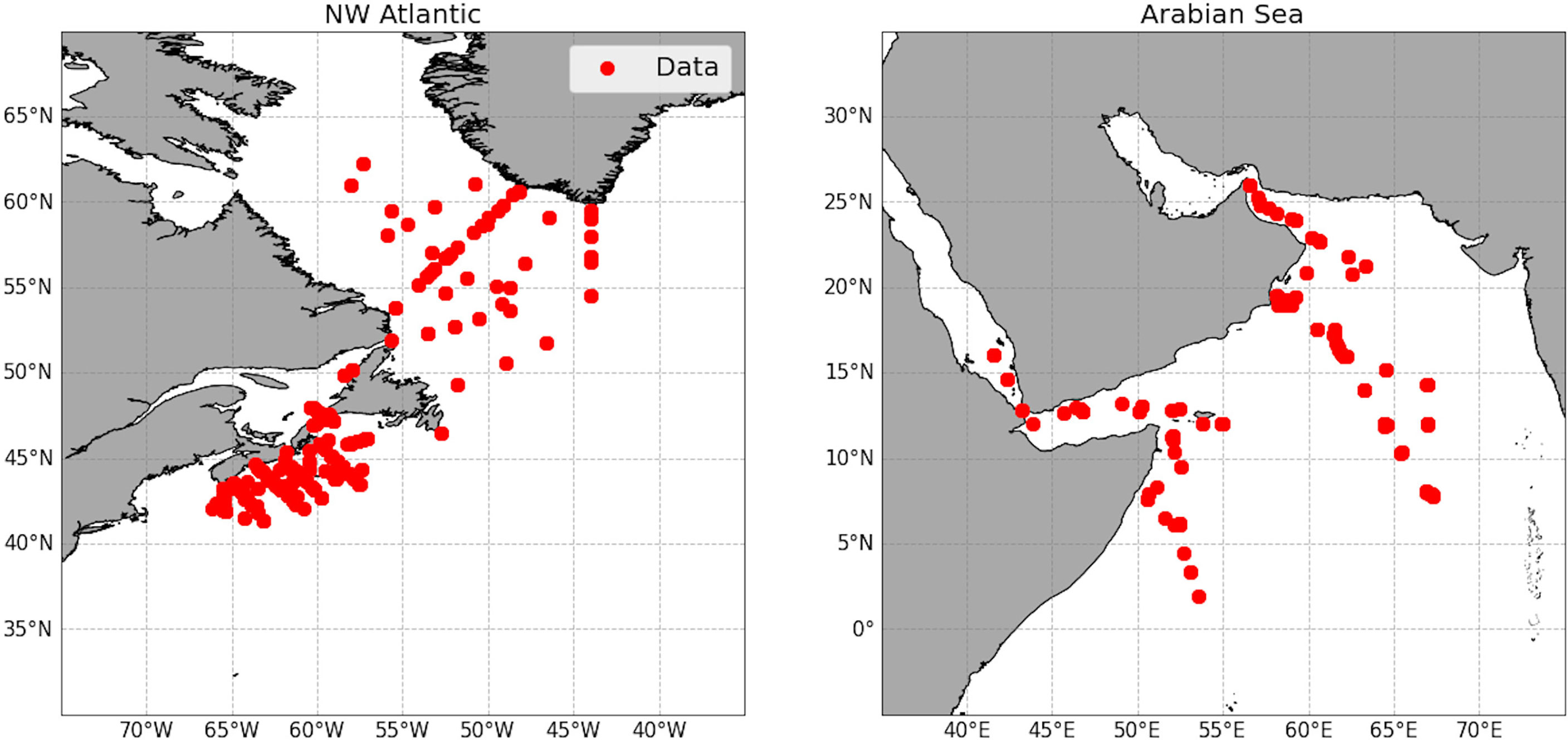
Figure 1 Maps of the sample collection sites for both the northwest Atlantic and the Arabian sea. Red dots indicate where the carbon and nitrogen data were located.
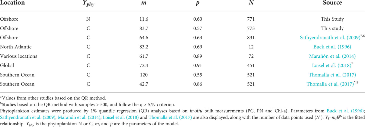
Table 1 Parameters of the power law relationship of carbon (C) and nitrogen (N) fitted against chlorophyll-a.
Water samples were collected with Niskin bottles from the euphotic zones (depth at which 99% of the surface light is absorbed) of the study sites. Over 90% of the samples were collected from <40 m below the water surface, whilst the remaining samples were from 40-80 m depth. Seawater (0.5-1.5 L) was filtered through a 25 mm GF/F filter prior to storage in liquid nitrogen at − 80 ∘ C (Stuart and Head, 2005). A Carbon, Hydrogen and Nitrogen (CHN) analyser was employed to derive the total PC and PN contents within the samples (Collos, 2002). These samples are expected to be composed predominantly of the particulate organic forms of C and N (i.e., POC and PON). Concentrations of Chl-a were measured using a Turner Designs fluorometer (Holm-Hansen et al., 1965) and high-performance liquid chromatography (HPLC) was adopted to derive accessory pigment compositions in addition to Chl-a. The total PC and PN compositions and Turner fluorometric Chl-a concentrations were used to compute the relationships between particulate carbon and Chl-a and particulate nitrogen and Chl-a. The elemental stoichiometry of bulk properties (e.g., PC:PN) was also estimated. The HPLC dataset was utilized as an independent set of measurements to distinguish phytoplankton functional groups dominating the samples. A fixed set of HPLC pigment criteria (as defined in Table 2 of Sathyendranath) allowed to discriminate the phytoplankton taxa present in each sample.
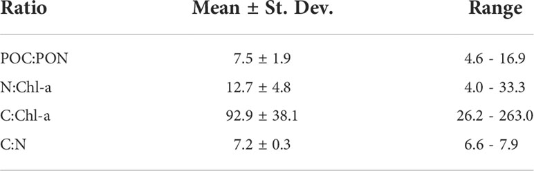
Table 2 Mean with standard deviation (St. Dev.) and range of POC:PON, phytoplankton N:Chl-a, C:Chl-a, and C:N, for concurrent data on POC, PON and Chl-a.
As evidenced above, measurements of total PC and PN can be straightforward to quantify. However, it is less practical to derive corresponding estimates of algal and non-algal fractions from bulk measures. The approach utilized in this study, first developed by Sathyendranath et al. (2009) for use in quantifying phytoplankton C, overcomes this challenge by attempting to derive information on the elemental composition of autotrophic plankton from total particulate C and N pools over a range of Chl-a concentrations. This method builds on the notion that changes in the non-autotrophic component of suspended materials alter the elemental content of a given observation without affecting its chlorophyll levels; hence, the lowest estimate of total PC or PN of any given Chl-a observation corresponds to the phytoplanktonic contribution to that element. Specifically, the phytoplankton C and N so obtained are the upper bound, in the sense that there would always be some non-autotrophic component present in the samples, which would bias the phytoplankton C and N upwards.
Prior to analysis, the PC, PN and Turner Chl-a sets of measurements were log-transformed to linearize the relationships observed and decrease the influence of samples with high values of different C, N and Chl-a in the regressions (see also Legendre and Michaud, 1999). PC and PN were treated as dependent variables and were first analyzed by a simple least-squares regression against Turner Chl-a, following standard practice (see Buck et al., 1996; Sathyendranath et al., 2009; Marañón et al., 2014; Thomalla et al., 2017). The fitted equations for total C and N are expressed as
where, Y is the predicted variable, B is Chl-a, and m and p are parameters of the power law model, and the subscript i denotes that the predicted variable (and parameters values for m and p ) are either with reference to total PC or PN. The equation can be expressed in linear format in log 10 space, as log 10 (Yi) = log 10 (mi) + pi log10(B), with log 10 (mi) and pi representing the intercept and slope of the linear regression, respectively.
Equation 1 was fitted using a quantile regression (QR) between the total Yi and Chl-a (B ), for both i = PC and PN. This allows the computation of a lower bound predominantly associated with the phytoplankton contribution to the element (either C or N), for a given Chl-a concentration. A 1% QR (q=0.01) was identified as the most appropriate quantile to define the lowest possible range of observations for phytoplanktonic contribution, following the q > 5/N criterion (N being the number of total observations), as suggested by Rogers (1993), and considering N = 773 for C and 771 for N. This method provides an upper limit of the phytoplankton contribution to the total particulate C and N pools. The results from QR analyses for both C and N were then combined to compute changes in the C:N ratio of phytoplankton as a function of Chl-a. Uncertainties in C:N were computed by running an ensemble of simulations over the Chl-a range, varying the four parameters (slope and intercept of the C and of N equations) between their confidence intervals in every permutation, and taking the minimum and maximum values. As described above, HPLC pigment composition data were used to examine the phytoplankton types present in the samples. Thus, taxonomic groups were further exploited to compute the stoichiometry of different algal groups using the parameterized model and HPLC Chl-a as inputs.
Following an initial inspection of log 10 scatter plots of PN and Chl-a, and PC and Chl-a, we observed that some unusual outliers in the data with surprisingly low PC and PN values for a given Chl-a concentration, relative to the entire dataset. The outliers were traced to three cruises. To avoid the influence of these discrepancies between the detected data points and the parent distribution on the subsequent investigations, samples from these three cruises were excluded from further analyses. All analyses for this study were carried out in Python and the quantile regressions were performed using the QuantReg package. This package estimates a QR model as a standard regression using iterative reweighted least squares. The uncertainties in the regression are also provided by default as an output from the analyses. An example Jupyter Notebook Python Script, processing the in-situ data and tuning the models is provided on this GitHub page (https://github.com/rjbrewin/POC-PON-Tchl-analysis).
The European Space Agency’s Ocean Colour Climate Change Initiative (ESA OC-CCI, Version 5.0) data were used in this study (Sathyendranath et al., 2019). This consists of a time-series of processed (bias-corrected and merged) ocean-colour data (for more information see https://climate.esa.int). Datasets from satellite observations of ocean colour are publicly accessible from https://www.oceancolour.org. Two 8-day composite maps of Chl-a with a 4 km by 4 km spatial resolution were generated for the Northwest Atlantic and the Arabian Sea study sites, corresponding to the 10-17 June 2006 and the 22-29 March 2005, respectively. These periods were selected as relatively cloud-free (<20% cover). Satellite outputs and results from this study were combined to produce a map of Chl-a, phytoplankton C, N and C:N ratio, for the two sampling sites within the selected periods. This further application illustrates how in-situ data can be exploited to derive simple methods for estimations of the distribution of phytoplankton elemental content and stoichiometry using remote sensing technology.
Upon regressing PC against Chl-a and PN against Chl-a from all data (see Figures 2A, D, 50% black lines), the overall correlations appeared highly significant (68% of the variation in PC was explained by Chl-a, with a P-value<0.001; 76% of the variation in PN was explained by Chl-a (P-value<0.001), and resulted in a mean conversion ratio of 211 for PC:Chl-a and 27.6 for PN:Chl-a. Slopes and intercepts between the 1% and 50% regressions were significantly different for PC (Figure 2A), with the 1% slope being steeper than the 50% slope (Figure 2C). The intercepts of the lower bound, 1%, and the upper bound, 50%, were significantly different for both PC and PN (Figures 2B, E), while a small overlap exists between the slopes of the PN regression (Figure 2F), related to larger uncertainties in the slope of the 1% quantile. The change in the slopes is such that the blue lines (1%) for both PC and PN converge towards the 50% percentile as the pigments reach higher concentrations. The slope of the 1% quantile regression for PN (0.60) was greater than that of C (0.57). The interpretation of the 1% quantile regression as being determined largely by phytoplankton C and N is consistent with the contributions of autotrophic C and N to total PC and PN increasing with Chl-a concentration, with highest contributions potentially during algal blooms conditions.
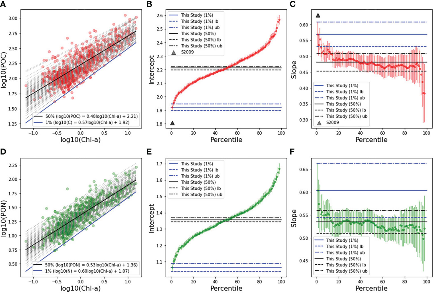
Figure 2 In-situ particulate carbon (top row) and nitrogen (bottom row), each plotted as a function of Turner chlorophyll-a from in-situ measurements. Least-squares fits to log 10 -transformed data, along with minimum carbon (Cphyto) and nitrogen (Nphyto) estimates by quantile regression (QR, q = 0.01) (A, D). Quantile regression lines (from 1 to 99%) are plotted in grey dotted lines. The 1% percentile is highlighted in blue and the 50th percentile in black. Intercepts (B, E) and slopes (C, F) for the different quantile fits, including error margins for each regression line. 1% QRs and uncertainties (upper bounds, ub and lower bounds, lb) are shown by the continuous, dashed and dash-dotted lines in blue, (middle and right panels), while Sathyendranath et al. (2009) carbon parameter values are also displayed (triangle, panels B, C).
Our premise is that the 1% quantile regressions can be used to estimate phytoplankton C and N from Chl-a, using Eq. 1 and the parameters m and p (Table 1, top two entries). For phytoplankton C, the parameters (Cphyto = 83.7B0.57, where B is Chl-a, Table 1) sit within the range of values reported in the literature. Notably, the intercept (m) matches the value presented in Buck et al. (1996). For the parameters produced in the phytoplankton N analysis (Nphyto = 11.6B0.6) there are no prior results in the literature to compare with. However, estimates obtained here for the N:Chl-a ratio (Table 2) are consistent with the range of values in the literature (Yentsch and Vaccaro, 1958; Manny, 1969; Verity, 1981; Staehr et al., 2002). Therefore, confidence that this model yields reasonable estimates of phytoplankton C and N from Chl-a can be gained, considering the good agreement between model parameters (m and p) for C derived here and those from other studies, and the broad agreement of N:Chl-a ratio values between this and earlier observations.
The 1% quantile regression models of phytoplankton C and N were used to estimate the C:N ratio as a function of Chl-a (Figure 3). Results suggest that the elemental stoichiometry of phytoplankton varies across the Chl-a range with the C:N ratio decreasing with increasing phytoplankton biomass, from around 8 at very low chlorophyll to 6 at high chlorophyll, intersecting the Redfield ratio towards higher phytoplankton biomass concentrations. This progression in the C:N ratio is consistent with the phytoplankton under oligotrophic conditions (low chlorophyll) being nitrogen limited, and those in eutrophic (high chlorophyll) conditions being nitrogen replete. However, the lower and upper bounds on the parameter estimates lead to considerable uncertainty margins (Figure 3), and suggest that results are not significantly different from Redfield over the Chl-a range studied. The C:N values are more robust over the intermediate concentrations along the chlorophyll range (where the majority of the Chl-a data is distributed), and the uncertainties are higher at the extremes where there is a smaller number of observations (Figure 3). Averages and ranges from the analysis, for all ratios, are provided in Table 2.
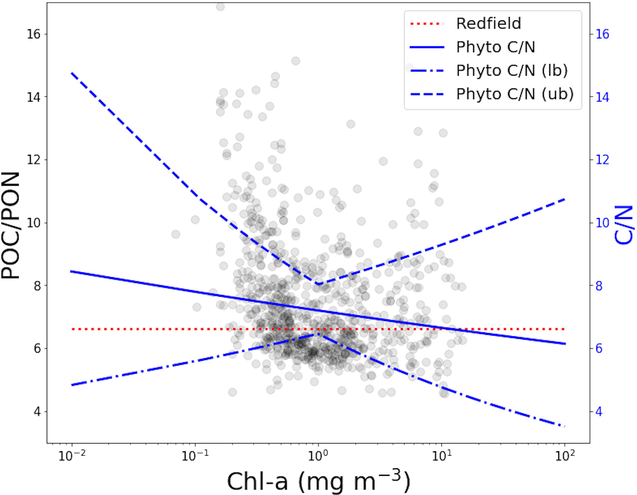
Figure 3 POC:PON against Chl-a showing the Redfield ratio (6.625, dotted red line), the phytoplankton C:N established by 1% QR regression analysis (blue line), and the relative uncertainties (upper bound, ub, dashedline line, and lower bound, lb, dot-dashedline).
Amongst the six distinct phytoplankton types examined, the diagnostic pigment analysis revealed some samples were dominated by diatoms, prymnesiophytes, Prochlorococcus, other picocyanobacteria (e.g. Synechococcus) or green algae. Dinoflagellates did not emerge as dominating any of the samples, according to the criteria applied. Differences were observed in the stoichiometry of the five phytoplankton groups that were identified (Figure 4; Table 3). The C:N ratios estimated were higher than the Redfield ratio. Diatoms were the closest group to the standard 6.6 Redfield ratio. Green algae and smaller phytoplankton types, on the other hand, displayed the highest stoichiometric values among all groups observed.
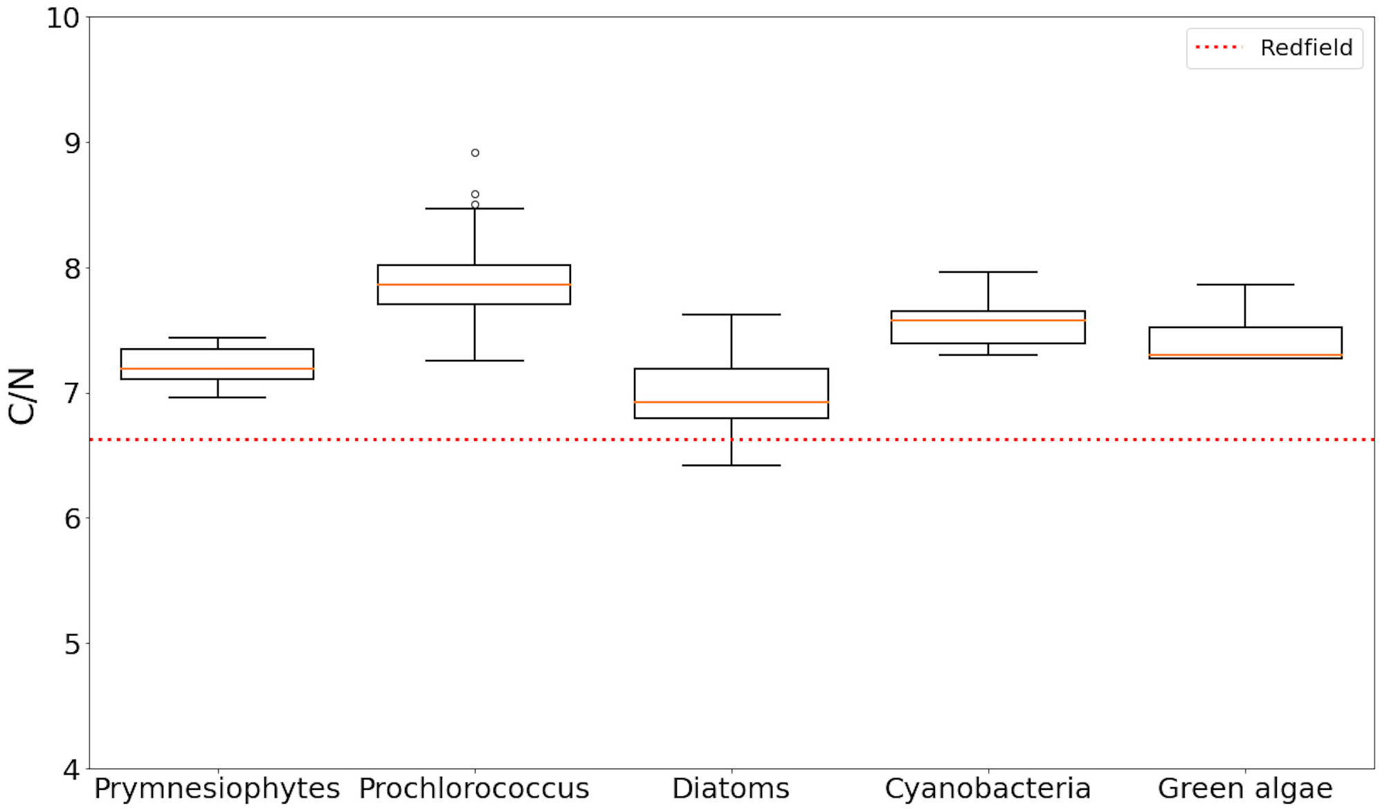
Figure 4 Boxplot of C:N ratios specific to the five phytoplankton taxa identified through HPLC analysis. Redfield ratio is highlighted by the dotted red line. See Table 3 for the mean and range of taxon-specific ratio.
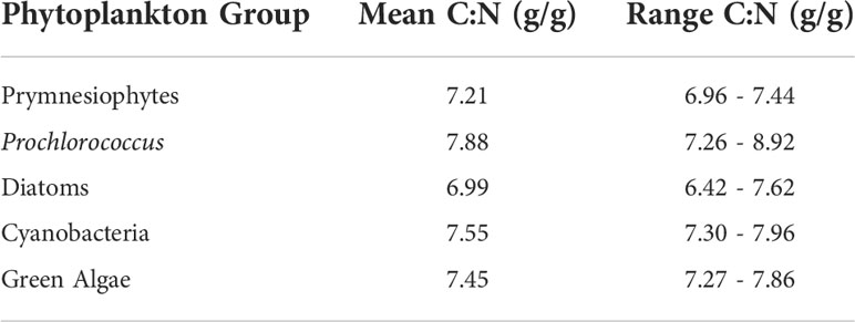
Table 3 Taxon-specific mean and range of phytoplankton C:N.
Using remotely-sensed Chl-a as input to our models (Eq. 1), the distributions of phytoplankton C, N, and C:N were computed for the NW Atlantic and the Arabian Sea study sites (Figure 5). The maps generated highlight the different biogeochemical areas within the NW Atlantic and the Arabian Sea during early summer 2006 and early spring 2005, respectively for the two sites. Observations for the Atlantic area coincided with the spring bloom season characterized by considerable variability in phytoplankton biomass, ranging from oligotrophic to eutrophic conditions. In contrast, the Arabian Sea biome has more stable and lower levels of Chl-a during the early spring. High concentrations of phytoplankton C and N only covered a small proportion of the areas shown, with the majority of the regions being low in phytoplankton biomass. Applying the model to satellite data allows the production of maps at a variety of scales, in time and space, to study the phytoplanktonic biomass and stoichiometry. However, one needs to be cautious interpreting the maps in conditions outside the range of data for which the model was parameterized, for example, in oligotrophic waters <0.07 mg m −3 Chl-a.
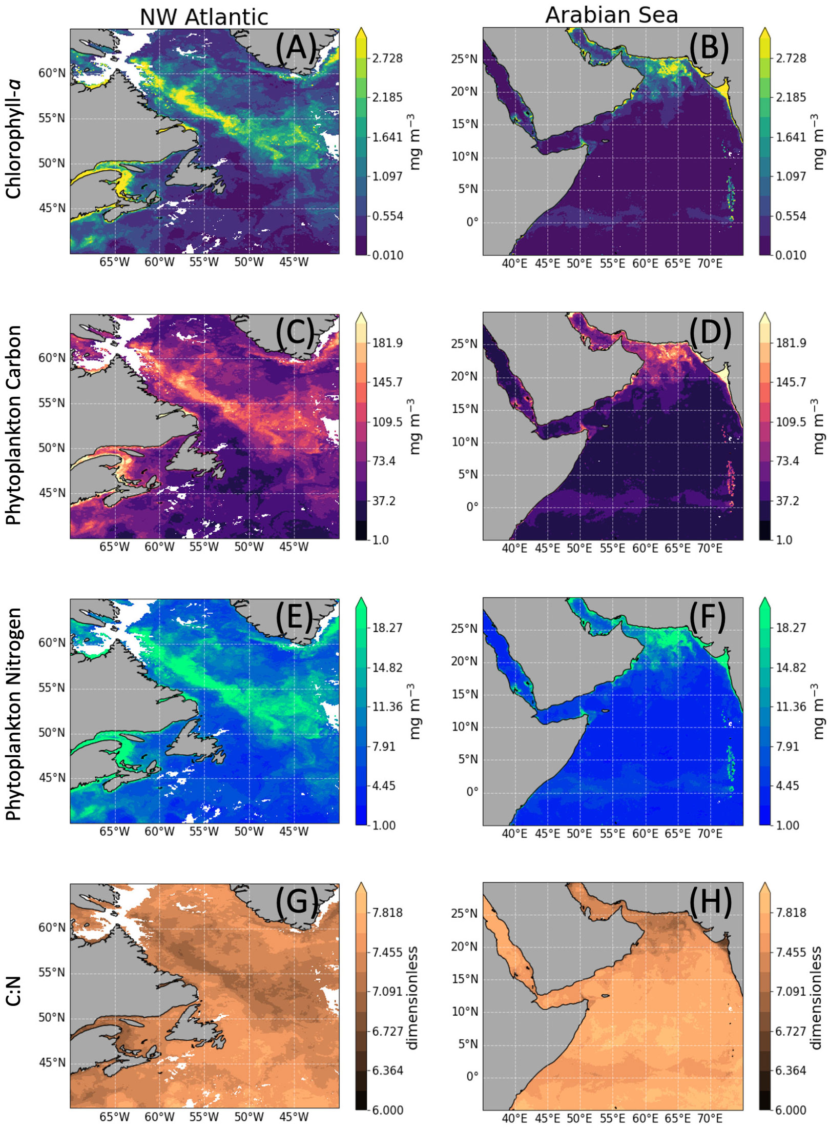
Figure 5 Satellite estimates of chlorophyll-a (A, B), quantile regression-derived autotrophic carbon (C, D) and nitrogen (E, F), and phytoplankton C:N ratio (G, H). Maps were generated based on remotely sensed OC-CCI chlorophyll data for an 8 day relatively clear sky composite of the Northwest Atlantic [10-17/06/2006, left-hand side panels (A, C, E, G)] and the Arabian Sea [22-29/03/2005, right-hand side panels (B, D, F, H)] with a 4 km spatial resolution.
Good linear correlations were found between the observed log10-transformed PON and Chl-a, and POC and Chl-a concentrations (Figures 2A, D). Expectedly, the parameters of the fit in the relationship between POC and Chl-a are in good agreement with those presented in Sathyendranath et al. (2009) considering similar data were used. Estimates of the POC:Chl-a ratio in this study (mean 211, range 33-1286) are broadly consistent with the literature (e.g., 100-1000; Legendre and Michaud, 1999; Stramski et al., 2008; Rasse et al., 2017). However, published analyses of particulate nitrogen, and how this varies with Chl-a, are generally less abundant and, thus, harder to compare against. Stoichiometric observations with a mean POC:PON ratio of 7.5 (Table 2) are also in agreement with Redfield’s findings (Tanoue and Handa, 1979; Sharp et al., 1980; Sterner et al., 2008; Frigstad et al., 2011; Frigstad et al., 2014). This value may appear high compared to previous observations, but differences can be attributed to the different statistical approaches used and lack of sampling replications that results in varying levels of total POC.
The overall values produced fit within traditional ranges and indirectly validate the model used; hence, this approach represents a simple and efficient solution for quantifying estimates of phytoplankton C and N at sea, as well as the ratio between the two, using remotely sensed Chl-a. The satellite data represent an opportunity to extrapolate these relationships over large spatial and temporal scales. Such relationships can also be useful for testing complex marine ecosystem models. Nonetheless, regional differences in model parameters are likely present, and one should be cautious about applying these models to satellite data in different regions and ranges of Chl-a outside those used to tune the models (Redfield et al., 1963; Körtzinger et al., 2001; Sterner et al., 2008; Martiny et al., 2013).
Autotrophic standing stock, primary production, export production and sequestration can be quantified by studying various metrics, such as phytoplankton carbon content, nitrogen content and chlorophyll concentration. Conversion factors are often adopted to evoke the measures desired and can be derived using controlled phytoplankton cultures. However, these experiments are unlikely to represent natural conditions (Flynn, 2003; Franks, 2009; Anderson et al., 2010). In field studies, bulk measures of C and N are generally easy to measure but distinguishing between the algal and non-algal contributions to these bulk elements is challenging due to operational constraints. Whereas phytoplankton C and N are often used as measures of phytoplankton biomass, standardized protocols of their direct measurement at sea have not been established yet; for this reason, indirect means are often invoked. Several studies have explored the use of a linear regression models of the POC and Chl-a relationship, to discriminate algal composition from that of non-autotrophic and detrital particles (Steele and Baird, 1961; Tett et al., 1975; Eppley et al., 1992; Behrenfeld et al., 2005; Frigstad et al., 2011), though they do not account for the nonlinearity of the Chl-a and POC relationship.
Other methods have been employed with various degrees of success, but none are reported to perform without limitations. The detection of phytoplankton C fractions from satellite imagery has been proposed as another approach for making indirect estimations. Behrenfeld et al. (2005) used a linear approach to derive the algal contribution to backscattering, by first subtracting a fixed value related to non-algal particles. Later studies refined this method to account for the variability of non-algal particles, but these either rely on several assumptions or cannot efficiently remove the impact of non-algal particles at higher algal concentrations, including bacteria, bubbles, and other particles (e.g. plastics). These models are difficult to cross-validate due to the paucity of in-situ phytoplankton C data (Dall’Olmo et al., 2009; Bellacicco et al., 2019). Poorly known distribution and physical characteristics of smaller particles further constrain the reliability of any modelling and contribute to the natural limitations inherent to the use of backscattering (Stramski et al., 2004; Organelli et al., 2018). Martínez-Vicente et al. (2013) and Graff et al. (2015) derived phytoplankton C directly from flow cytometry, the former using phytoplankton abundances, cellular carbon per unit volume and mean cell volume. However, these models either rely on estimations from lab-based studies or are time-consuming and limited to samples analyzed by flow cytometry. A cell volume model has also served for conversions to retrieve phytoplankton N (Montagnes et al., 1994; Sun and Liu, 2003). An earlier investigation used the chlorosis levels in phytoplankton cells to obtain indirect estimates on their organic N concentration at sea based on the inverse relationship between the nitrogen:chlorophyll and the carotenoid:chlorophyll ratios (Yentsch and Vaccaro, 1958) using estimates from controlled experiments. Alternatively, the quantile regression approach used here and adopted from Sathyendranath et al. (2009) applies a nonlinear regression to the particulate N or C compositions fitted against Chl-a concentrations to account for the varying relationships between variables. Fixed ratios are frequently invoked in many global-scale studies (Aumont and Bopp, 2006; Follows et al., 2007; Dutkiewicz et al., 2009) even though deviations are well documented in the elemental composition of phytoplankton (Droop, 1983). The extent to which these ratios diverge from standard proportions have significant implications for the parametrization of these models and, consequently, for simulations of the N and C cycles, C-transfer efficiency up the food web, and air-sea gas exchange (Sterner and Elser, 2002; Ayata et al., 2013). The approach presented here, represents a simple avenue to estimating elemental ratios and stoichiometry in phytoplankton.
The variability in the phytoplankton C:Chl-a and N:Chl-a ratios can be explained as a direct result of changes in the physiological status of autotrophs. Algal organisms are not strictly homeostatic, and ambient conditions (e.g., availability of nutrients, light, and depth levels) can stimulate the regulation of their metabolism (i.e., respiration, exudation and storage), resulting in the acclimation of the photosynthetic apparatus – alteration of nutrient use efficiency and adjustment of Chl-a content. The net difference between acquisition and losses can lead to the consequent decoupling of cellular C, N and pigment contents in seemingly adaptive ways (Berman-Frank and Dubinsky, 1999). Environmental conditions also impact the phytoplankton community composition, representing an additional factor determining stoichiometry (Clark et al., 2013; Talmy et al., 2014). Alternatively, the rationale of the QR approach develops on the notion that variability in total PC and PN within any given concentration of Chl-a is primarily associated with the variability of non-autotrophic particles. Ultimately, the relationship between phytoplankton C and N fitted against the Chl-a concentration range can be used to explore the stoichiometry of natural autotrophic composition in the sea utilizing a simple method that exploits straightforward concepts. Furthermore, the empirical models developed here (Table 1) can be of use to verify results from more complex marine ecosystem models where the phytoplankton C:chl-a and N:chl-a ratios are emergent properties of the simulations (de Mora et al., 2016). Data used were derived from up to 40 m below the water surface and spanned a range of trophic conditions across different biomes. Outputs should therefore be interpreted as representative of the surface mixed layer.
The mean C:Chl-a and N:Chl-a ratios derived using the QR model are consistent with previous observations, for C (Verity, 2002; Lefèvre et al., 2003; Lü et al., 2009; Xiu and Chai, 2012; Jakobsen and Markager, 2016; Martínez-Vicente et al., 2017) and for N (Yentsch and Vaccaro, 1958; Manny, 1969; Verity, 1981; Staehr et al., 2002). Both the phytoplankton C and N to Chl-a fits display steeper slopes than their corresponding particulate regression (50% QR), suggesting an increasing contribution to PC and PN can be associated with phytoplankton at higher Chl-a concentrations. Thomalla et al. (2017) attempted to retrieve phytoplankton C adopting different methods including the QR, using the same dataset in some instances. They find that the range and distributions from the QR approach compare remarkably well with those generated using backscattering techniques based on both Stramski (1999) and Behrenfeld et al. (2005) approaches, reconciling the two techniques and supporting the use of the QR approach.
The phytoplankton C:N trend decreases from low to high chlorophyll waters, a direct result of the steeper slope in the relationship between phytoplankton N and Chl-a than phytoplankton C and Chl-a (0.60 > 0.57). Considerable uncertainties were observed over the extreme ends of the chlorophyll axis in this fit, challenging the accuracy of estimates and their applicability to real world scenarios (Figure 3). Nonetheless, the mean and range values are in broad agreement with earlier investigations (Körtzinger et al., 2001; Geider and La Roche, 2002; Staehr et al., 2002; Frigstad et al., 2011; Frigstad et al., 2014; Wagner et al., 2019). Stoichiometry estimates yielded are above the canonical 6.625 for most of the chlorophyll range, before approaching Redfield ratio and dropping below it at higher Chl-a. This inclination further emphasizes the argument that adopting a constant ratio to estimate elemental compositions of autotrophic cells are likely to lead to erroneous outcomes. Thus, we can speculate that the C:N ratio of phytoplankton in the surface mixed layer is highest when the algal biomass is lowest and it decreases as bloom conditions are approached, while its range remains close to Redfield across most of the chlorophyll axis.
The results from this study also show variations in C:N amongst phytoplankton groups. The taxon-specific ratios that emerge from these analyses were predominantly above or close to the Redfield ratio. This variance in the elemental composition between phytoplankton types may be associated with a difference in cell size (Morel and Bricaud, 1981; Grover, 1991; Tozzi et al., 2004; Griffiths and Harrison, 2009; Talmy et al., 2014), their nutritional status and cell activity (Klausmeier et al., 2004b; Halsey and Jones, 2015). The nutrient storage capacity of autotrophic cells is known to be size dependent. For example, diatoms can store large nutrient concentrations contributing to lower C:N ratio than small celled autotrophs in a nutrient replete environment as supported by wider phytoplankton culture studies (Lomas and Gilbert, 2000; Bertilsson et al., 2003; Heldal et al., 2003; Martiny et al., 2013). Thus, variations in stoichiometry with phytoplankton community composition can also play an important role in determining the bulk stoichiometry of phytoplankton. It could be speculated that a higher mean ratio could be induced by a possible dominance of small-celled autotrophs over diatoms. It is reasonable to assume that our results are subject to variation based on the dominant phytoplankton species within each community. However, for the same species, links between the cellular C and N content can be further modulated by metabolic functions (e.g., diverging rates of carbon fixation and nutrient acquisition), as previously mentioned.
This uncoupling can manifest in a response to factors not accounted for in this method, including alterations of nutrient and light availability and temperature (vertically and horizontally) (Verity, 1981; Behrenfeld et al., 2002; Staehr et al., 2002; Frigstad et al., 2011; Jackson et al., 2017). Environment conditions can influence metabolic functions in algal organisms encouraging adaptive mechanisms (acclimation), which may lead to bias in estimations if not accounted for. A change in the ratio can also be expected below the euphotic region (Schneider et al., 2003; Martiny et al., 2013). Phytoplankton estimates from remotely sensed chlorophyll will also benefit from incorporating per-pixel uncertainties, included in the satellite data, by propagating errors and producing supplementary maps reporting the quality of satellite products (Brewin et al., 2017; Martínez-Vicente et al., 2017; Sathyendranath et al., 2017). The QR method could also be applied to other limiting nutrients and elements, such as phosphorus and iron. Finally, considering the influence of stoichiometric variations on the dynamics of food webs, global nutrient and carbon cycling, and the Earth’s climate, it is critical that we improve our understanding of phytoplankton C and N, and how these metrics vary in the ocean.
Despite the progress made and the new technologies developed in recent years, our understanding of the phytoplankton elemental composition at sea is still unsatisfactory. The ability to produce accurate measures of algal contribution to particulate N and C in the sea from bulk properties measured directly in the field is challenging, for both traditional and modern methods. Considering the global oceans and the atmosphere are expected to be increasingly affected by anthropogenic influences, better understanding of the elemental composition of phytoplankton is needed.
In this study, we analyzed a large dataset of the total particulate C and N and Chl-a in the NW Atlantic and the Indian Ocean to compute the phytoplankton N:Chl-a, C:Chl-a and C:N ratios, and their variations over the observed Chl-a range through the use of a simple and straightforward method. Results suggest that phytoplankton contribution to PC and PN increases with an increase in its biomass. Conversely, the phytoplankton C:N ratio decreases with increases in biomass. Stoichiometry of phytoplankton was further observed to follow taxon-specific variations, as demonstrated in the wider literature. Estimates generated here agree with the range of values from previous laboratory and field studies, and earlier applications of this method on different datasets have generated comparable results. Therefore, it can be deduced that the simple approach adopted here can be used to achieve reasonable results, and the estimates it produces could serve to test complex ecosystem models. The established ratios, combined with satellite-derived Chl-a can be used to estimate the phytoplankton C, N, C:N and their spatial distributions, demonstrating an immediate application of the model. Future replications of this method will benefit from the inclusion of additional elements, such as the particulate organic phosphorous or iron. Observations over a wider geographical scale could further assess the broad applicability of this method.
The in-situ datasets and code used for data processing can be found in the following GitHub repository https://github.com/rjbrewin/POC-PON-TChl-analysis. This includes an Jupyter Notebook Python Script, that can be run through binder (https://mybinder.org) without having to install Python software. Datasets from satellite observations of ocean colour are publicly accessible from https://www.oceancolour.org.
SS provided the data and came up with the concept, with input from RB. GM and RB synthesized the data, ran the analysis and prepared the figures. GM wrote the first version of the manuscript, with input from RB, and prepared all tables. All authors contributed to the subsequent versions of the manuscript.
This work was supported through a European Space Agency (ESA) project “Biological Pump and Carbon Exchange Processes (BICEP)” and by the Simons Foundation Project “Collaboration on Computational Biogeochemical Modeling of Marine Ecosystems (CBIOMES)” (549947, SS). It was also supported by the UK National Centre for Earth Observation (NCEO). Additional support from the Ocean Colour Component of the Climate Change Initiative of the European Space Agency (ESA) is gratefully acknowledged. RB is funded by a UKRI Future Leader Fellowship (MR/V022792/1).
We acknowledge all those involved in the collection of data used in this study. This work was supported by a MSc project in Conservation and Biodiversity in the College of Life and Environmental Sciences, University of Exeter.
The authors declare that the research was conducted in the absence of any commercial or financial relationships that could be construed as a potential conflict of interest.
All claims expressed in this article are solely those of the authors and do not necessarily represent those of their affiliated organizations, or those of the publisher, the editors and the reviewers. Any product that may be evaluated in this article, or claim that may be made by its manufacturer, is not guaranteed or endorsed by the publisher.
Anderson L. G., Tanhua T., Björk G., Hjalmarsson S., Jones E. P., Jutterstr öm S., et al. (2010). Arctic Ocean shelf-basin interaction : An active continent shelf CO2 pump and its impact on the degree of calcium carbonate solubility. Deep Sea Res. Part I: Oceanographic Res. Papers 57, 869–879. doi: 10.1016/J.DSR.2010.03.012
Aumont O., Bopp L. (2006). Globalizing results from ocean in situ iron fertilization studies. Global Biogeochemical Cycles 20, 1–15. doi: 10.1029/2005GB002591
Ayata S. D., Lévy M., Aumont O., Sciandra A., Sainte-Marie J., Tagliabue A., et al. (2013). Phytoplankton growth formulation in marine ecosystem models: Should we take into account photo-acclimation and variable stoichiometry in oligotrophic areas? J. Mar. Syst. 125, 29–40. doi: 10.1016/J.JMARSYS.2012.12.010
Banse K. (1977). Determining the carbon-to-chlorophyll ratio of natural phytoplankton. Mar. Biol. 41, 199–212. doi: 10.1007/BF00394907
Behrenfeld M., Boss E., Siegel D. A., Shea D. M. (2005). Carbon-based ocean productivity and phytoplankton physiology from space. Global Biogeochemical Cycles 19, 1–14. doi: 10.1029/2004GB002299
Behrenfeld M. J., Marañón E., Siegel D. A., Hooker S. B. (2002). Photoacclimation and nutrient-based model of light-saturated photosynthesis for quantifying oceanic primary production. Mar. Ecol. Prog. Ser. 228, 103–117. doi: 10.3354/MEPS228103
Bellacicco M., Vellucci V., Scardi M., Barbieux M., Marullo S., D’ortenzio F. (2019). Quantifying the impact of linear regression model in deriving bio-optical relationships: The implications on ocean carbon estimations. Sensors 19, 3032. doi: 10.3390/S19133032
Berman-Frank I., Dubinsky Z. (1999). Balanced growth in aquatic plants: Myth or reality? Phytoplankton use the imbalance between carbon assimilation and biomass production to their strategic advantage. BioScience 49, 29–37. doi: 10.1525/BISI.1999.49.1.29
Bertilsson S., Berglund O., Karl D. M., Chisholm S. (2003). Elemental composition of marine Prochlorococcus and Synechococcus: Implications for the ecological stoichiometry of the sea. W. Limnology Oceanography 48, 1721–1731. doi: 10.4319/LO.2003.48.5.1721
Brewin R. J. W., Ciavatta S., Sathyendranath S., Jackson T., Tilstone G., Curran K., et al. (2017). Uncertainty in ocean-color estimates of chlorophyll for phytoplankton groups. Front. Mar. Sci. 4. doi: 10.3389/FMARS.2017.00104
Brewin R. J. W., Sathyendranath S., Platt T., Bouman H., Ciavatta S., Dall’Olmo G., et al. (2021). Sensing the ocean biological carbon pump from space: A review of capabilities, concepts, research gaps and future developments. Earth-Science Rev. 217, 103604. doi: 10.1016/J.EARSCIREV.2021.103604
Buck K. R., Chavez F. P., Campbell L. (1996). Basin-wide distributions of living carbon components and the inverted trophic pyramid of the central gyre of the north Atlantic ocean, summer 1993. Aquat. Microbial Ecol. 10, 283–298. doi: 10.3354/AME010283
Chai F., Dugdale R. C., Peng T. H., Wilkerson F. P., Barber R. T. (2002). One-dimensional ecosystem model of the equatorial pacific upwelling system. Part I: model development and silicon and nitrogen cycle. Deep Sea Res. Part II: Topical Stud. Oceanography 49, 2713–2745. doi: 10.1016/S0967-0645(02)00055-3
Clark J. R., Lenton T. M., Williams H. T. P., Daines S. J. (2013). Environmental selection and resource allocation determine spatial patterns in picophytoplankton cell size. Limnology Oceanography 58, 1008–1022. doi: 10.4319/LO.2013.58.3.1008
Collos Y. (2002). “Determination of particulate carbon and nitrogen in coastal waters,” In Pelagic ecology methodology. Subba Rao DV (A.A. Balkema Publishers, Tokyo), 333–341.
Dall’Olmo G., Westberry T. K., Behrenfeld M. J., Boss E., Slade W. H. (2009). Significant contribution of large particles to optical backscattering in the open ocean. Biogeosciences 6, 947–967. doi: 10.5194/BG-6-947-2009
Dearman J. R., Taylor A. H., Davidson K. (2003). Influence of autotroph model complexity on simulations of microbial communities in marine mesocosms. Mar. Ecol. Prog. Ser. 250, 13–28. doi: 10.3354/MEPS250013
de Mora L., Butensch ön M., Allen J. I. (2016). The assessment of a global marine ecosystem model on the basis of emergent properties and ecosystem function: a case study with ERSEM. Geoscientific Model. Dev. 9, 59–76. doi: 10.5194/GMD-9-59-2016
Doney S. C., Glover D. M., Najjar R. G. (1996). A new coupled, one-dimensional biological-physical model for the upper ocean: Applications to the JGOFS Bermuda Atlantic time-series study (BATS) site. Deep-Sea Res. Part II: Topical Stud. Oceanography 43, 591–624. doi: 10.1016/0967-0645(95)00104-2
Droop M. R. (1983). 25 years of algal growth kinetics: A personal view. Botanica Marina 26, 99–112. doi: 10.1515/BOTM.1983.26.3.99
Dutkiewicz S., Follows M. J., Bragg J. G. (2009). Modeling the coupling of ocean ecology and biogeochemistry. Global Biogeochemical Cycles 23, 1–15. doi: 10.1029/2008GB003405
Eppley R. W., Chavez F. P., Barber R. T. (1992). Standing stocks of particulate carbon and nitrogen in the equatorial Pacific at 150° W. J. Geophysical Res. 97, 655–661. doi: 10.1029/91JC01386
Falkowski P. G. (1994). The role of phytoplankton photosynthesis in global biogeochemical cycles. Photosynthesis Res. 39, 235–258. doi: 10.1007/BF00014586
Falkowski P. G. (2012). Ocean science: The power of plankton. Nature 483, S17–S20. doi: 10.1038/483s17a
Falkowski P. G., Laws E. A., Barber R. T., Murray J. W. (2003). Phytoplankton and their role in primary, new, and export production. In Ocean Biogeochemistry. Global Change — The IGBP Series. Ed. Fasham M.J.R.. (Springer, Berlin, Heidelberg), 99–121. doi: 10.1007/978-3-642-55844-3
Flynn K. J. (2003). Do we need complex mechanistic photoacclimation models for phytoplankton? Limnology Oceanography 48, 2243–2249. doi: 10.4319/LO.2003.48.6.2243
Flynn K. J. (2010). Ecological modelling in a sea of variable stoichiometry: Dysfunctionality and the legacy of redfield and monod. Prog. Oceanography 84, 52–65. doi: 10.1016/J.POCEAN.2009.09.006
Follows M. J., Dutkiewicz S., Grant S., Chisholm S. W. (2007). Emergent biogeography of microbial communities in a model ocean. Science 315, 1843–1846. doi: 10.1126/SCIENCE.1138544/SUPPL_FILE/FOLLOWS-SOM.PDF
Franks P. J. S. (2009). Planktonic ecosystem models: perplexing parameterizations and a failure to fail. J. Plankton Res. 31, 1299–1306. doi: 10.1093/PLANKT/FBP069
Frigstad H., Andersen T., Bellerby R. G. J., Silyakova A., Hessen D. O. (2014). Variation in the seston C:N ratio of the Arctic ocean and pan-Arctic shelves. J. Mar. Syst. 129, 214–223. doi: 10.1016/J.JMARSYS.2013.06.004
Frigstad H., Andersen T., Hessen D. O., Naustvoll L. J., Johnsen T. M., Bellerby R. G. J. (2011). Seasonal variation in marine C:N:P stoichiometry: Can the composition of seston explain stable redfield ratios? Biogeosciences 8, 2917–2933. doi: 10.5194/BG-8-2917-2011
Furuya K. (1990). Subsurface chlorophyll maximum in the tropical and subtropical western pacific ocean: Vertical profiles of phytoplankton biomass and its relationship with chlorophyll-a and particulate organic carbon. Mar. Biol. 107, 529–539. doi: 10.1007/BF01313438
Geider R. J., La Roche J. (2002). Redfield revisited: Variability of C:N:P in marine microalgae and its biochemical basis. Eur. J. Phycology 37, 1–17. doi: 10.1017/S0967026201003456
Goebel N. L., Edwards C. A., Zehr J. P., Follows M. J. (2010). An emergent community ecosystem model applied to the California current system. J. Mar. Syst. 83, 221–241. doi: 10.1016/J.JMARSYS.2010.05.002
Graff J. R., Milligan A. J., Behrenfeld M. J. (2012). The measurement of phytoplankton biomass using flow-cytometric sorting and elemental analysis of carbon. Limnology Oceanography: Methods 10, 910–920. doi: 10.4319/LOM.2012.10.910
Graff J. R., Westberry T. K., Milligan A. J., Brown M. B., Dall’Olmo G., van Dongen-Vogels V., et al. (2015). Analytical phytoplankton carbon measurements spanning diverse ecosystems. Deep Sea Res. Part I: Oceanographic Res. Papers 102, 16–25. doi: 10.1016/J.DSR.2015.04.006
Griffiths M. J., Harrison S. T. L. (2009). Lipid productivity as a key characteristic for choosing algal species for biodiesel production. J. Appl. Phycology 21, 493–507. doi: 10.1007/S10811-008-9392-7
Grover J. P. (1991). Resource competition in a variable environment: Phytoplankton growing according to the variable-internal-stores model. Am. Nat. 138, 811–835. doi: 10.1086/285254
Halsey K. H., Jones B. M. (2015). Phytoplankton strategies for photosynthetic energy allocation. Annu. Rev. Mar. Sci. 7, 265–297. doi: 10.1146/annurev-marine-010814-015813
Heldal M., Scanlan D. J., Norland S., Thingstad F., Mann N. H. (2003). Elemental composition of single cells of various strains of marine Prochlorococcus and Synechococcus using x-ray microanalysis. Limnology Oceanography 48, 1732–1743. doi: 10.4319/lo.2003.48.5.1732
Holm-Hansen O., Lorenzen C. J., Holmes R. W., Strickland J. D. H. (1965). Fluorometric determination of chlorophyll. ICES J. Mar. Sci. 30, 3–15. doi: 10.1093/ICESJMS/30.1.3
Jackson T., Sathyendranath S., Platt T. (2017). An exact solution for modeling photoacclimation of the carbon-to-chlorophyll ratio in phytoplankton. Front. Mar. Sci. 4. doi: 10.3389/FMARS.2017.00283
Jakobsen H. H., Markager S. (2016). Carbon-to-chlorophyll ratio for phytoplankton in temperate coastal waters: Seasonal patterns and relationship to nutrients. Limnology Oceanography 61, 1853–1868. doi: 10.1002/LNO.10338
Karl D. M., Björkman K. M., Dore J. E., Fujieki L., Hebel D. V., Houlihan T., et al. (2001). Ecological nitrogen-to-phosphorus stoichiometry at station ALOHA. Deep Sea Res. Part II: Topical Stud. Oceanography 48, 1529–1566. doi: 10.1016/S0967-0645(00)00152-1
Klausmeier C. A., Litchman E., Daufreshna T., Levin S. A. (2004a). Optimal nitrogen-to-phosphorus stoichiometry of phytoplankton. Nature 429, 171–174. doi: 10.1038/nature02454
Klausmeier C. A., Litchman E., Levin S. A. (2004b). Phytoplankton growth and stoichiometry under multiple nutrient limitation. Limnology Oceanography 49, 1463–1470. doi: 10.4319/LO.2004.49.4_PART_2.1463
Körtzinger A., Koeve W., Kähler P., Mintrop L. (2001). C:N ratios in the mixed layer during the productive season in the northeast Atlantic ocean. Deep Sea Res. Part I: Oceanographic Res. Papers 48, 661–688. doi: 10.1016/S0967-0637(00)00051-0
Kwiatkowski L., Aumont O., Bopp L., Ciais P. (2018). The impact of variable phytoplankton stoichiometry on projections of primary production, food quality, and carbon uptake in the global ocean. Global Biogeochemical Cycles 32, 516–528. doi: 10.1002/2017GB005799
Lefèvre N., Taylor A. H., Gilbert F. J., Geider R. J. (2003). Modeling carbon to nitrogen and carbon to chlorophyll a ratios in the ocean at low latitudes: Evaluation of the role of physiological plasticity. Limnology Oceanography 48, 1796–1807. doi: 10.4319/LO.2003.48.5.1796
Legendre L., Michaud J. (1999). Chlorophyll a to estimate the particulate organic carbon available as food to large zooplankton in the euphotic zone of oceans. J. Plankton Res. 21, 2067–2083. doi: 10.1093/PLANKT/21.11.2067
Litchman E., de Tezanos Pinto P., Edwards K. F., Klausmeier C. A., Kremer C. T., Thomas M. K. (2015). Global biogeochemical impacts of phytoplankton: A trait-based perspective. J. Ecol. 103, 1384–1396. doi: 10.1111/1365-2745.12438
Li W. K. W., Zohary T., Yacobi Y. Z., Wood A. M. (1993). Ultraphytoplankton in the eastern Mediterranean Sea: towards deriving phytoplankton biomass from flow cytometric measurements of abundance, fluorescence and light scatter. Mar. Ecol. Prog. Ser. 102, 79–87. doi: 10.3354/MEPS102079
Llewellyn C. A. (2004). Phytoplankton community assemblage in the English channel: a comparison using chlorophyll a derived from HPLC-CHEMTAX and carbon derived from microscopy cell counts. J. Plankton Res. 27, 103–119. doi: 10.1093/plankt/fbh158
Loisel H., Duforêt-Gaurier L., Dessailly S., Sathyendranath S., Evers-King H., Vantrepotte V., et al. (2018). A satellite view of the particulate organic carbon and its algal and non-algal carbon pools. In Proceedings of the Ocean Optics XXIV, Dubrovnik, Croatia, 7–12.
Lomas M. W., Gilbert P. M. (2000). Comparisons of nitrate uptake, storage, and reduction in marine diatoms and flagellates. J. Phycology 36, 903–913. doi: 10.1046/J.1529-8817.2000.99029.X
Lü S., Wang X., Han B. (2009). A field study on the conversion ratio of phytoplankton biomass carbon to chlorophyll- a in jiaozhou bay, china. Chin. J. Oceanology Limnology 27, 793–805. doi: 10.1007/S00343-009-9221-0
Manny B. A. (1969). The relationship between organic nitrogen and the carotenoid to chlorophyll a ratio in five freshwater phytoplankton species. Limnology Oceanography 14, 69–79. doi: 10.4319/LO.1969.14.1.0069
Marañón E., Cermeño P., Huete-Ortega M., López-Sandoval D. C., Mouriño Carballido B., Rodríguez-Ramos T. (2014). Resource supply overrides temperature as a controlling factor of marine phytoplankton growth. PloS One 9, e99312. doi: 10.1371/JOURNAL.PONE.0099312
Martínez-Vicente V., Dall’Olmo G., Tarran G., Boss E., Sathyendranath S. (2013). Optical backscattering is correlated with phytoplankton carbon across the Atlantic Ocean. Geophysical Res. Lett. 40, 1154–1158. doi: 10.1002/grl.50252
Martínez-Vicente V., Evers-King H., Roy S., Kostadinov T. S., Tarran G. A., Graff J. R., et al. (2017). Intercomparison of ocean color algorithms for picophytoplankton carbon in the ocean. Front. Mar. Sci. 4. doi: 10.3389/fmars.2017.00378
Martiny A. C., Vrugt J. A., Primeau F. W., Lomas M. W. (2013). Regional variation in the particulate organic carbon to nitrogen ratio in the surface ocean. Global Biogeochemical Cycles 27, 723–731. doi: 10.1002/GBC.20061
Montagnes D. J., Berges J. A., Harrison P. J., Taylor F. J. (1994). Estimating carbon, nitrogen, protein, and chlorophyll a from volume in marine phytoplankton. Limnology Oceanography 39, 1044–1060. doi: 10.4319/lo.1994.39.5.1044
Moore C. M., Mills M. M., Arrigo K. R., Berman-Frank I., Bopp L., Boyd P. W., et al. (2013). Processes and patterns of oceanic nutrient limitation. Nat. Geosci. 6, 701–710. doi: 10.1038/ngeo1765
Morel A., Bricaud A. (1981). Theoretical results concerning light absorption in a discrete medium, and application to specific absorption of phytoplankton. Deep Sea Res. Part A. Oceanographic Res. Papers 28, 1375–1393. doi: 10.1016/0198-0149(81)90039-X
Olson R. J., Shalapyonok A., Sosik H. M. (2003). An automated submersible flow cytometer for analyzing pico- and nanophytoplankton: FlowCytobot. Deep-Sea Res. Part I: Oceanographic Res. Papers 50, 301–315. doi: 10.1016/S0967-0637(03)00003-7
Organelli E., Dall’Olmo G., Brewin R. J. W., Tarran G. A., Boss E., Bricaud A. (2018). The open-ocean missing backscattering is in the structural complexity of particles. Nat. Commun. 9, 1–11. doi: 10.1038/s41467-018-07814-6
Phinney D. A., Yentsch C. S. (1985). A novel phytoplankton chlorophyll technique: toward automated analysis. J. Plankton Res. 7, 633–642. doi: 10.1093/PLANKT/7.5.633
Platt T., Sathyendranath S. (1988). Oceanic primary production: Estimation by remote sensing at local and regional scales. Science 241, 1613–1620. doi: 10.1126/SCIENCE.241.4873.1613
Rasse R., Dall’Olmo G., Graff J., Westberry T. K., van Dongen-Vogels V., Behrenfeld M. J. (2017). Evaluating optical proxies of particulate organic carbon across the surface Atlantic Ocean. Front. Mar. Sci. 4, 367. doi: 10.3389/fmars.2017.00367
Redfield A. C. (1934). On the proportions of organic derivatives in sea water and their relation to the composition of plankton. James Johnstone Memorial Volume (University Press Liverpool), 1, 176–192.
Redfield A. C., Ketchum B. H., Richards F. (1963). The influence of organisms on the composition of sea water. sea 2, 26–77.
Sardans J., Janssen I. A., Ciais P., Obersteiner M., Peñuelas J. (2021). Recent advances and future research in ecological stoichiometry. Perspect. Plant Ecology Evol. Systematics 50, 125611. doi: 10.1016/j.ppees.2021.125611
Sathyendranath S., Brewin R. J. W., Brockmann C., Brotas V., Calton B., Chuprin A., et al. (2019). An ocean-colour time series for use in climate studies: The experience of the ocean-colour climate change initiative (OC-CCI). Sensors 19, 4285. doi: 10.3390/S19194285
Sathyendranath S., Brewin R. J. W., Jackson T., Mélin F., Platt T. (2017). Ocean-colour products for climate-change studies: What are their ideal characteristics? Remote Sens. Environ. 203, 125–138. doi: 10.1016/J.RSE.2017.04.017
Sathyendranath S., Platt T., Kovač Ž., Dingle J., Jackson T., Brewin R. J. W., et al. (2020). Reconciling models of primary production and photoacclimation. Appl. Optics 59, C100–C114. doi: 10.1364/AO.386252
Sathyendranath S., Stuart V., Nair A., Oka K., Nakane T., Bouman H., et al. (2009). Carbon-to-chlorophyll ratio and growth rate of phytoplankton in the sea. Mar. Ecol. Prog. Ser. 383, 73–84. doi: 10.3354/meps07998
Schneider B., Schlitzer R., Fischer G., N othig E.-M. (2003). Depth-dependent elemental compositions of particulate organic matter (POM) in the ocean. Global Biogeochemical Cycles 17, 1–16. doi: 10.1029/2002GB001871
Schoo K. L., Malzahn A. M., Krause E., Boersma M. (2013). Increased carbon dioxide availability alters phytoplankton stoichiometry and affects carbon cycling and growth of a marine planktonic herbivore. Mar. Biol. 160, 2145–2155. doi: 10.1007/S00227-012-2121-4
Sciandra A. (1991). Coupling and uncoupling between nitrate uptake and growth rate in prorocentrum minimum (Dinophyceae) under different frequencies of pulsed nitrate supply. Mar. Ecol. Prog. Ser. 72, 261–269. doi: 10.3354/MEPS072261
Sharp J. H., Perry M. J., Renger E. H., Eppley R. W. (1980). Phytoplankton rate processes in the oligotrophic waters of the central north Pacific Ocean. J. Plankton Res. 2, 335–353. doi: 10.1093/PLANKT/2.4.335
Staehr P. A., Henriksen P., Markager S. (2002). Photoacclimation of four marine phytoplankton species to irradiance and nutrient availability. Mar. Ecol. Prog. Ser. 238, 47–59. doi: 10.3354/meps238047
Steele J. H., Baird I. E. (1961). Relations between primary production, chlorophyll and particulate carbon. Limnology Oceanography 6, 68–78. doi: 10.4319/lo.1961.6.1.0068
Sterner R. W., Andersen T., Elser J. J., Hessen D. O., Hood J. M., McCauley E., et al. (2008). Scale-dependent carbon:nitrogen:phosphorus seston stoichiometry in marine and freshwaters. Limnology Oceanography 53, 1169–1180. doi: 10.4319/LO.2008.53.3.1169
Sterner R. W., Elser J. J. (2002). Ecological stoichiometry: the biology of elements from molecules to the biosphere (Princeton University Press, Princeton, New Jersey).
Stramski D. (1999). Refractive index of planktonic cells as a measure of cellular carbon and chlorophyll a content. Deep Sea Res. Part I: Oceanographic Res. Papers 46, 335–351. doi: 10.1016/S0967-0637(98)00065-X
Stramski D., Boss E., Bogucki D., Voss K. J. (2004). The role of seawater constituents in light backscattering in the ocean. Prog. Oceanography 61, 27–56. doi: 10.1016/J.POCEAN.2004.07.001
Stramski D., Reynolds R. A., Babin M., Kaczmarek S., Lewis M. R., Röttgers R., et al. (2008). Relationships between the surface concentration of particulate organic carbon and optical properties in the eastern south Pacific and eastern Atlantic oceans. Biogeosciences 5, 171–201. doi: 10.5194/bg-5-171-2008
Strickland J. D. H. (1960). Measuring the production of marine phytoplankton. Bull. Fisheries Res. Board Canada 122, 1–172.
Stuart V., Head E. (2005). The BIO method. In The 2nd SeaWiFS HPLC analysis round-robin experiment (SeaHARRE-2). Ed. Hooker SB. NASA/TM 2005-212785, Greenbelt, MD, 112.
Sun J., Liu D. (2003). Geometric models for calculating cell biovolume and surface area for phytoplankton. J. Plankton Res. 25, 1331–1346. doi: 10.1093/plankt/fbg096
Talmy D., Blackford J., Hardman-Mountford N. J., Polimene L., Follows M. J., Geider R. J. (2014). Flexible C:N ratio enhances metabolism of large phytoplankton when resource supply is intermittent. Biogeosciences 11, 4881–4895. doi: 10.5194/BG-11-4881-2014
Tanoue E., Handa N. (1979). Distribution of particulate organic carbon and nitrogen in the Bering Sea and northern north pacific ocean. Journal of the oceanographical society of Japan 35, 47–62. doi: 10.1007/BF02108282
Tett P., Cottrell J. C., Trew D. O., Wood B. J. B. (1975). Phosphorus quota and the chlorophyll: carbon ratio in marine phytoplankton1. Limnology Oceanography 20, 587–603. doi: 10.4319/LO.1975.20.4.0587
Thomalla S. J., Ogunkoya A. G., Vichi M., Swart S. (2017). Using optical sensors on gliders to estimate phytoplankton carbon concentrations and chlorophyll-to-carbon ratios in the Southern Ocean. Front. Mar. Sci. 4. doi: 10.3389/FMARS.2017.00034
Tozzi S., Schofield O., Falkowski P. (2004). Historical climate change and ocean turbulence as selective agents for two key phytoplankton functional groups. Mar. Ecol. Prog. Ser. 274, 123–132. doi: 10.3354/MEPS274123
Verity P. G. (1981). Effects of temperature, irradiance, and daylength on the marine diatom Leptocylindrus danicus cleve. Photosynthesis and cellular composition. J. Exp. Mar. Biol. Ecol. 55, 79–91. doi: 10.1016/0022-0981(81)90094-0
Verity P. G. (2002). A decade of change in the skidaway river estuary II. particulate organic carbon, nitrogen, and chlorophyll a. Estuaries 25, 961–9750. doi: 10.1007/BF02691344
Wagner H., Jebsen C., Wilhelm C. (2019). Monitoring cellular C:N ratio in phytoplankton by means of FTIR-spectroscopy. J. Phycology 55, 543–551. doi: 10.1111/JPY.12858
Xiu P., Chai F. (2012). Spatial and temporal variability in phytoplankton carbon, chlorophyll, and nitrogen in the North Pacific. J. Geophysical Research: Oceans 117, 11023. doi: 10.1029/2012JC008067
Yentsch C. S., Menzel D. W. (1963). A method for the determination of phytoplankton chlorophyll and phaeophytin by fluorescence. Deep Sea Res. Oceanographic Abstracts 10, 221–231. doi: 10.1016/0011-7471(63)90358-9
Keywords: nitrogen, carbon, chlorophyll-a, Redfield, phytoplankton, satellite
Citation: Maniaci G, Brewin RJW and Sathyendranath S (2022) Concentration and distribution of phytoplankton nitrogen and carbon in the Northwest Atlantic and Indian Ocean: A simple model with applications in satellite remote sensing. Front. Mar. Sci. 9:1035399. doi: 10.3389/fmars.2022.1035399
Received: 02 September 2022; Accepted: 10 October 2022;
Published: 09 November 2022.
Edited by:
Griet Neukermans, Ghent University, BelgiumReviewed by:
Márcio Silva de Souza, Federal University of Rio Grande, BrazilCopyright © 2022 Maniaci, Brewin and Sathyendranath. This is an open-access article distributed under the terms of the Creative Commons Attribution License (CC BY). The use, distribution or reproduction in other forums is permitted, provided the original author(s) and the copyright owner(s) are credited and that the original publication in this journal is cited, in accordance with accepted academic practice. No use, distribution or reproduction is permitted which does not comply with these terms.
*Correspondence: Robert J. W. Brewin, ci5icmV3aW5AZXhldGVyLmFjLnVr
Disclaimer: All claims expressed in this article are solely those of the authors and do not necessarily represent those of their affiliated organizations, or those of the publisher, the editors and the reviewers. Any product that may be evaluated in this article or claim that may be made by its manufacturer is not guaranteed or endorsed by the publisher.
Research integrity at Frontiers
Learn more about the work of our research integrity team to safeguard the quality of each article we publish.