 Xian-Rong Cen
 Shuang-Xi Guo
 Yan Wang4
 Sheng-Qi Zhou
- 1State Key Laboratory of Tropical Oceanography, South China Sea Institute of Oceanology, Chinese Academy of Sciences, Guangzhou, China
- 2School of Industrial Design and Ceramic Art, Foshan University, Foshan, China
- 3Southern Marine Science and Engineering Guangdong Laboratory (Guangzhou), Guangzhou, China
- 4Department of Ocean Science and Center for Ocean Research in Hong Kong and Macau, Hong Kong University of Science and Technology, Hong Kong, Hong Kong SAR, China
Turbulence within the upper ocean mixed layer plays a key role in various physical, biological, and chemical processes. Between September and November 2011, a dataset of 570 vertical profiles of the turbulent kinetic energy (TKE) dissipation rate, as well as conventional hydrological and meteorological data, were collected in the upper layer of the tropical Indian Ocean. These data were used to statistically analyze the vertical distribution of the TKE dissipation rate in the mixed layer. The arithmetic-mean method made the statistical TKE dissipation rate profile more scattered than the median and geometric-mean methods. The statistical TKE dissipation rate were respectively scaled by the surface buoyancy flux and the TKE dissipation rate at the mixed-layer base. It was found that the TKE dissipation rate scaled by that at the mixed-layer base exhibited better similarity characteristics than that scaled by the surface buoyancy flux, whether the stability parameter D/|LMO| was greater or less than 10, indicating that the TKE dissipation rate at the mixed-layer base is a better characteristic scaling parameter for reflecting the intrinsic structure of the TKE dissipation rate in the mixed layer, where D and LMO are respectively the mixed-layer thickness and the Monin-Obukhov length scale. The parameterization of the TKE dissipation rate at the mixed-layer base on the shear-driven dissipation rate and the surface buoyancy flux was further explored. It was found that the TKE dissipation rate at the mixed-layer base could be well fitted by a linear combination of three terms: the wind-shear-driven dissipation rate, the surface buoyancy flux, and a simple nonlinear coupling term of these two .
1 Introduction
The upper part of the ocean is directly mixed by momentum and buoyancy fluxes from the atmosphere. This mixing produces a turbulent and homogeneous layer with a thickness of tens to hundreds of meters, commonly referred to as the upper ocean mixed layer (Kantha and Clayson, 2000; Pellichero et al., 2017). The upper ocean mixed layer acts as a buffer between the atmosphere and the interior ocean and affects oceanic dynamic processes at various scales and eventually global climate change (Macdonald and Wunsch, 1996; Kantha and Clayson, 2000; Esters et al., 2018; Qiu et al., 2019; Meredith and Garabato, 2021). For example, turbulence in the mixed layer generally dominates mass and energy exchange between the atmosphere and the ocean (Qiu et al., 2016; Evans et al., 2018), adjusts the spatial distributions of various materials and water masses in the upper ocean (Esters et al., 2017), and facilitates absorption of excess heat and carbon dioxide from the atmosphere (Sabine et al., 2004). The mixed layer is also where certain water masses form through dynamic processes such as subduction and deep convection. These processes can further impact the water mass properties of the deeper ocean and hence the Meridional Overturning Circulation (Kostov et al., 2014; Zhang and Wang, 2018).
Turbulence plays an important role in the formation and evolution of the mixed layer. The associated turbulent structures are assumed to be controlled by energy input and exchange from the atmosphere. There are three main types of this external energy source (Thorpe, 2005). The first is wind stress, which drives turbulence by vertical mean-current shear based on the Kelvin-Helmholtz instabilities and transfers the momentum flux downward in the mixed layer (Callaghan et al., 2014). Based on the theory of the turbulent boundary layer, it is assumed that the vertical distribution of the wind-shear-driven dissipation rate satisfies the classical “law of the wall” (D'Asaro, 2014). The second source is the surface wave field. The dynamic processes of the surface wave field, such as wave-breaking and Langmuir convection, modify the turbulence characteristics of the upper ocean and convert the energy of the wave field into TKE (Thorpe, 2005; Wain et al., 2015). It has been reported that the surface wave field can significantly enhance turbulence only in the top few meters of the ocean (Gemmrich and Farmer, 2004). In this depth range, however, collected turbulence data in field observations are often contaminated by the vibration and wake of the vessel (Oakey and Elliott, 1982; Lombardo and Gregg, 1989; Brainerd and Gregg, 1993). The third source is surface buoyancy flux. During nighttime, surface cooling promotes the transfer of ocean heat to the atmosphere, thus convective instability leads to turbulent flows in the mixed layer (hereafter, the oceanic heat loss is defined as the positive buoyancy flux). In contract to the surface wave field driving turbulence within the top few meters, the surface buoyancy flux can convectively drive turbulence from the sea surface to the base of the mixed layer. However, during daytime, the ocean is heated by penetrating solar radiation, and the surface buoyancy flux acts as a sink for turbulence, which initiates stable stratification near the surface and thus suppresses turbulence (Anis and Moum, 1994; Moulin et al., 2018).
The TKE dissipation rate, ϵ, acts as an important sink in the energy budget of the global ocean. It balances the energy input to the ocean from external forcing (Wunsch and Ferrari, 2004; Ferrari and Wunsch, 2009). Regardless of the top few meters, which are dominated by surface waves, the mixed layer is thought to be affected mainly by wind-induced current shear and buoyancy flux, and the vertical distribution of TKE dissipation rate in the mixed layer has been widely studied and parameterized by a linear combination of the shear-driven dissipation rate and surface buoyancy flux (Lombardo and Gregg, 1989; Tedford et al., 2014; Esters et al., 2017; Esters et al., 2018). Field observations have indicated that in the mixed layer the TKE dissipation rate first decreases rapidly beneath the sea surface, and then remains relatively uniform towards the mixed-layer base (Shay and Gregg, 1986; Lombardo and Gregg, 1989; Anis and Moum, 1994; Moum and Rippeth, 2009). To identify the similarity structure of TKE dissipation rate in the mixed layer, it has usually been rendered dimensionless by surface buoyancy flux, , and has been found to be convergentin some ocean regions and in the atmosphere (Shay and Gregg, 1986; Moum and Rippeth, 2009; D'Asaro, 2014). These results have significantly expanded the understanding of turbulence structures in the mixed layer. Nonetheless, the choice of surface buoyancy flux as the scaling parameter may have some inherent flaws. For example, during daytime, surface buoyancy flux is inapplicable because it is negative and suppresses turbulence in the mixed layer. Moreover, when using only surface buoyancy flux to make TKE dissipation rate dimensionless, the contribution of wind-induced current shear is explicitly omitted, which may fail to produce a true intrinsic structure of TKE dissipation rate in the mixed layer (Anis and Moum, 1994; Lozovatsky et al., 2005). These issues motivate the search for a more appropriate parameter to characterize ϵ in the mixed layer.
In this paper, we attempt to propose a new characteristic parameter to reflect the intrinsic similarity structure of the TKE dissipation rate in the mixed layer. This parameter is available all day long, and its relationship with wind-induced current shear and surface buoyancy flux is systematically examined using the present dataset collected in the tropical Indian Ocean.
2 Theory and methods
2.1 Shear-driven dissipation rate ϵs
The oceanic surface wind-induced current shear stress τ0, as a function of the wind speed at a reference height and the drag coefficient, can be expressed (Jones and Toba, 2001) as
where ρa is the air density, CD is the drag coefficient, and U10 is the wind speed at a height of 10 m above the sea surface. Typical values of CD are on the order of 10-3 and depend on wind speed. The calculation of CD is based on version 3.0 of the Coupled Ocean-Atmosphere Response Experiment (COARE 3.0) bulk algorithm (Fairall et al., 1996; Fairall et al., 2003; Edson et al., 2013), which can be accessed at ftp://ftp1.esrl.noaa.gov/BLO/Air-Sea/bulkalg/cor3_0/. The friction velocity on the sea side, u*, which is a characteristic velocity reflecting boundary shear effect, is defined as
where ρ is the density of seawater.
When only wind stress is applied, based on the flat rigid-wall approximation of the ocean surface, in the upper boundary layer, the vertical distribution of the horizontal mean velocity U satisfies the classical logarithmic law (Esters et al., 2018)
where z0 is the roughness length of the sea surface boundary layer, z is distance from the sea surface, and κ=0.41 is the von Karman constant. This formula gives the velocity shear as . Thus, the dissipation rate dominated by wind stress alone follows the so-called “law of the wall” as
where reflects the balance between near-surface Reynolds stress and surface wind stress, and u′ and w′ are the fluctuating velocities in the horizontal and vertical directions.
2.2 Buoyancy flux
The oceanic surface buoyancy flux, which is affected by both heat and mass exchange between the atmosphere and ocean, is defined (Shay and Gregg, 1986; Thorpe, 2005) as
where g is the gravitational acceleration, ρ0 is the reference density of seawater, and Qp is the density flux, which is made up of contributions from temperature flux FT and freshwater flux FS as
Here, FT = -Qnet/ρwCp and , where α and β are the thermal expansion and saline contraction coefficients respectively. Cp represents the specific heat of seawater, and E, P, and S represent evaporation, precipitation, and sea surface salinity respectively. Qnet, the net radiative heat flux at the ocean surface, is given (Shay and Gregg, 1986) by the sum of the incoming shortwave radiation (SW), longwave radiation (LW), sensible heat (SH), and latent heat (LH) as
E, P, SW, and LW were measured directly by the onboard meteorological observation system, and SH and LH were computed using the general flux algorithm of COARE 3.0 (Fairall et al., 2003), which has been wildly used to estimate sensible and latent heat in the air-sea interaction community with accuracy within 5% for wind speed of 0-10 m s-1 and 10% for wind speed of 10-20 m s-1, guaranteeing a reasonable evaluation of .
2.3 TKE dissipation rate ϵ
TKE dissipation rate ϵ characterizes the conversion intensity of turbulent energy into heat through fluid viscous forces. In isotropic turbulence, ϵ is defined (Wolk et al., 2002) as
where v is Molecular viscosity coefficient, and is the velocity shear and directly measured by the shear probe mounted on the microstructure profiler. φ(k) is the shear spectrum in wavenumber (k) space, which were transformed from the frequency (f) space based on Taylor’s frozen turbulence hypothesis for each vertical segment.
Considering the observation noise in the high wave number region, the observed shear spectrum φ(k) is fitted with the theoretical Nasmyth spectrum φN(k) and extrapolated to high and low wavenumbers for each segment. φN(k) is given (Bluteau et al., 2016) by
where kv=(∈/v3)1/4 is Kolmogorov wavenumber. Thus, ϵ is then obtained by integrating the fitted Nasmyth spectrum over the full extrapolated wavenumber range (Moum et al., 1995).
2.4 Determination of the mixed layer depth
The mixed layer has a relatively homogeneous distribution of temperature, salinity, and density, resulting from turbulent mixing driven by the surface forcing. Its thickness, called as the mixed layer depth (MLD), is a basic scale in the study of the turbulent energy budget within the mixed layer. The threshold method, which is based on the changes in temperature and density or in their gradients, is a simple and extensively employed method to identify the MLD (Brainerd and Gregg, 1995; de Boyer Montégut et al., 2004). However, this method is somewhat subjective and not suitable for different regions and seasons (Brainerd and Gregg, 1995; de Boyer Montégut et al., 2004; Holte and Talley, 2009). Whereafter, some relatively objective methods were proposed, such as the curvature method (Lorbacher et al., 2006), split-merge method (Thomson and Fine, 2003), maximum angle method (Chu and Fan, 2011), and relative variance method (Huang et al., 2018). Huang et al. (2018) compared these objective methods and found that they have their own advantages in different regions and environments. In this study, the MLD is determined from the density profiles with the maximum angle method, which is based on the maximum angle between two depth vectors of the profile (de Boyer Montégut et al., 2004; Chu and Fan, 2011).
2.5 in the mixed layer
The input of surface energy makes the upper mixed layer be approximately vertically uniform layer. However, the energy flux varies with increasing depth as it transports downwards, resulting in a variable vertical structure of turbulence in the mixed layer. Based on the energy budget, the TKE dissipation rate ϵ is commonly used to represent turbulence in the mixed layer. Generally, the vertical structure of the nondimensionalized TKE dissipation rate, , versus nondimensionalized depth, z/D, has been widely investigated in the previous literature, where z is depth and D is the thickness of the mixed layer. This normalization method for ϵ basically requires that data be available at night, i.e., , which is favorable for convective mixing in the mixed layer. For example, Shay and Gregg (1986) performed a statistical analysis of using microstructure data collected in the Bahamas and the Gulf Stream warm core ring. They found that in the uppermost layer (5–10 m), the TKE dissipation rate ϵ was exceptionally high. This thin layer with enhanced ϵ was thought to be generated mainly by wind forcing and/or surface wave breaking. Below this thin layer, ϵ was nearly uniform in the mixed layer, with an average of 0.61 in the Bahamas and 0.72 in the Gulf Stream warm core ring. Lombardo and Gregg (1989) carried out a mixed-layer dynamic experiment at (34°N, 127°W), located in the outer reaches of the California Current. They found that the average value of in the mixed layer was 0.58. Anis and Moum (1994) analyzed a mixed-layer dataset collected in the Pacific Ocean in 1987. They found that decreased in an almost linear fashion with increasing depth in the lower half of the mixed layer, with a slight increase at the base of the mixed layer (i.e., near z/D~1). In a recent study Esters et al. (2018) statistically analyzed the scaled ϵ in mixed layer and found were scattered in five different surveyed sea areas. To address this inconsistency of and explore the similarity of ϵ in the mixed layer, in this study we try to propose a new characteristic parameter, TKE dissipation rate at the mixed-layer base ϵD, to normalize ϵ.
2.6 Data description
The observational dataset was acquired during an international field campaign, called the Cooperative Indian Ocean Experiment on Intraseasonal Variability in the Year 2011 (CINDY2011). This field campaign was part of the Dynamics of the Madden-Julian Oscillation (DYNAMO) program. For detailed information on CINDY2011, please refer to Yoneyama et al. (2013). The present study used only the on-board data collected by the research vessel MIRAI, which was stationed at (8°S, 80.5°E) (shown with the star in Figure 1). This measurement covered two periods, 30 September to 24 October and 30 October to 28 November 2011.
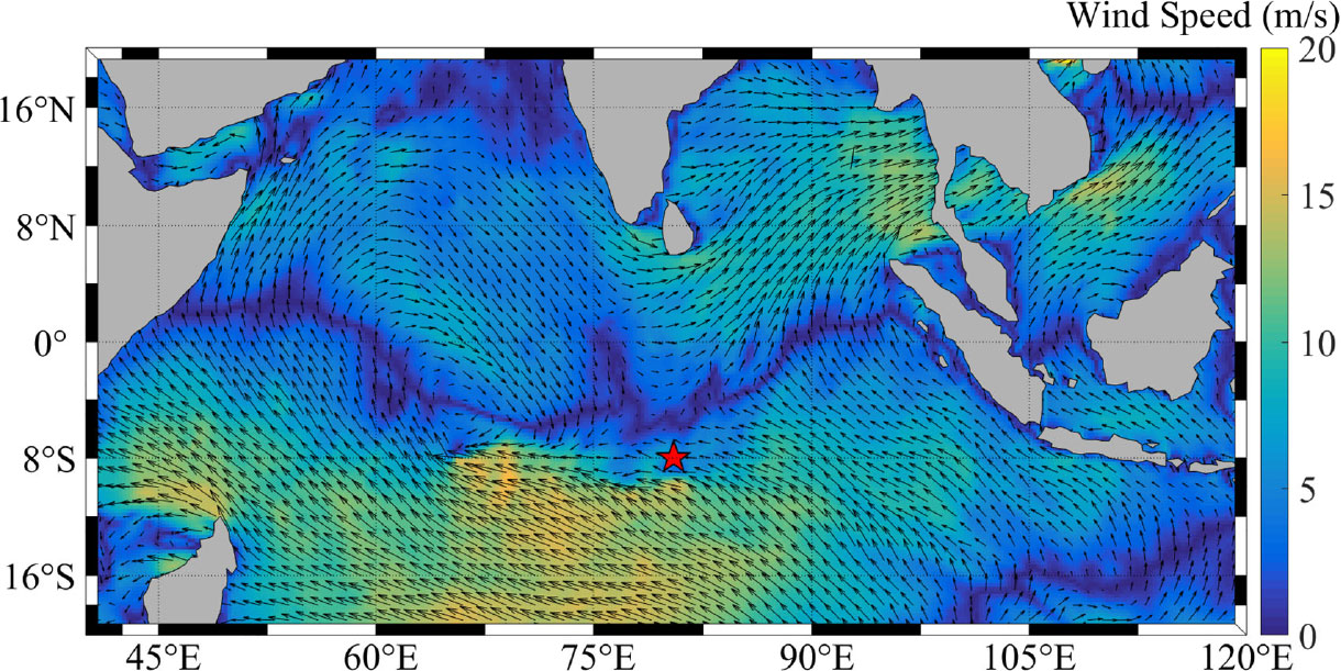
Figure 1 Map of the tropical Indian Ocean. The red star shows the fixed site where the dataset used in this study was collected. The contour and vector indicate the wind field at 10 m height above the sea surface on 30 September 2011 (i.e., the first day of the field campaign), which is from the ECMWF ERA5 reanalysis wind data at https://cds.climate.copernicus.eu/cdsapp#!/dataset/reanalysis-era5-pressure-levels?tab=overview.
The oceanic surface meteorological data collected on MIRAI included air and sea surface temperatures, wind speed at 10 m height, evaporation, precipitation, and solar radiation, and had a temporal resolution of 10 minutes. The wind profile was measured by a 915-MHz wind profiler (Yoneyama et al., 2013). Using the method described in the last section, the time series of wind stress τ0 and buoyancy flux are shown in Figures 2A, B. It is found that is positive and nearly constant at night except for the time of sunset and sunrise. During daytime, the heat gain is dominated by short-wave radiation, and varies sharply, increasing from zero after sunrise, reaching its maximum value near noon, and returning to zero again before sunset.
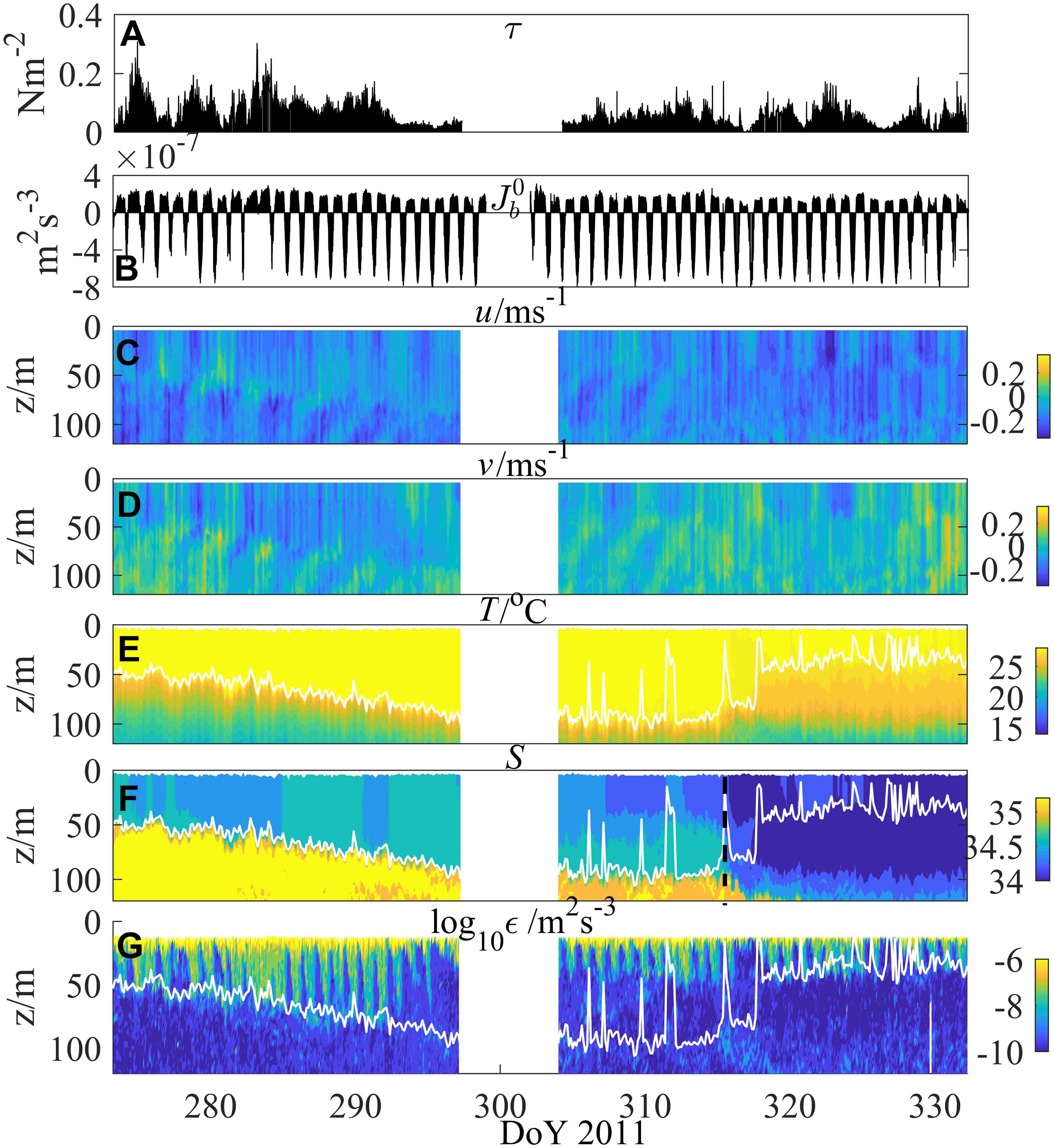
Figure 2 Time series of (A) wind stress, (B) surface buoyancy flux, (C) zonal current, (D) meridional current, (E) temperature, (F) salinity, and (G) TKE dissipation rate at the observation site. The white curves denote the base of the mixed layer. The black dashed line in (F) indicates that the data after DoY 315 (November 11) were not used due to the intrusion of a low-salinity water mass in the upper layer.
Conventional hydrographic instruments, including conductivity-temperature-depth (CTD) and the Lowered Acoustic Doppler Current Profiler (LADCP), were deployed down to 500 m every 3 h (Figures 2C–F). These data were postprocessed into vertical bins of 1 m for the CTD and 2 m for the LADCP. The base of the mixed layer is marked as the white curve in Figures 2E–G. It is of the order of magnitude of tens of meters in depth and shows obvious diurnal variations. This diurnal variation of MLD is one of the most important features of mixed layer. During the nighttime, cooling increases density of the surface water, which sinks and causes rapid turbulent convection, resulting in the increase of the MLD. While during the daytime, surface heating causes restratification and suppresses the turbulent convection, resulting in the decrease of the MLD (Imberger, 1985).
After each cast of CTD/LADCP, two microstructure profiles were measured consecutively by a Turbulence Ocean Microstructure Acquisition Profiler (TurboMAP) for the upper 300 m. To avoid contamination by vessel-generated motion, the microstructure data for the uppermost 10 m were discarded in post-processing analysis. Briefly, the observed shear spectra were fitted with the Nasmyth spectrum for each 2-m vertical segment, and then ϵ was obtained by integrating the fitted spectrum over the full extrapolated wavenumber range (Moum et al., 1995) [for further details of estimating ϵ, refer to Wolk et al. (2002)]. Figure 2G shows the time series of ϵ profiles.
Note, as shown in Figure 2F, that a water-mass intrusion with low temperature and low salinity occurred in the upper layer (0–100 m) from DoY (day of year) 315 (11 November 2011, see the dashed line in Figure 2F), which was also described by Seiki et al. (2013). This lateral dominant process was beyond the scope of this study, and all the datasets after that day were excluded. Therefore, a total of 285 CTD/LADCP and 570 microstructure profiles were included in the final analysis. For consistency, the microstructure data were further averaged according to the CTD profile time stamps. This complete, high-resolution dataset for both atmospheric and oceanic states made it possible to quantitatively analyze the dynamics of the ocean mixed layer.
3 Results
3.1 ϵ scaled with the surface buoyancy flux,
Although the previous studies show that the nondimensionalized TKE dissipation rate does not reflect very good similarity structure in mixed layer, we still first followed and examined the previous literature to study in the mixed layer during nighttime for the present dataset. The dataset includes 183 original ϵ profiles overall. Each profile was divided into vertical bins with size 0.05z/D. In each bin, the median, geometric-mean, and arithmetic-mean values and their corresponding 50% confidence intervals (i.e., the first and third quartiles) were calculated. Figure 3A shows versus z/D using these three statistical averaging methods. The median and geometric-mean values were found to agree roughly with each other, but significantly differed from the arithmetic-mean values. This is because the median and geometric-mean values represent a typical value of the dataset, and are not shewed by a small proportion of extremely large ϵ in the mixed layer. Moreover, the arithmetic-mean values were more scattered than the other statistical average values. To quantitatively evaluate which statistic gave the best representation of the present dataset, a scatter index SI was defined as
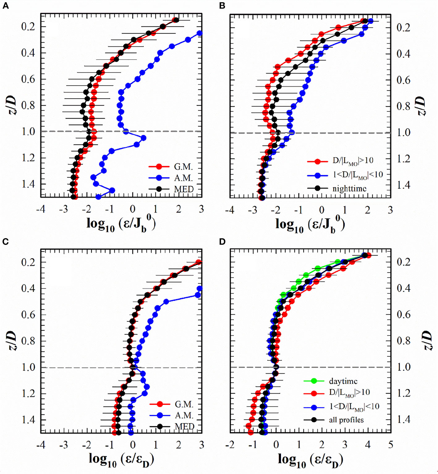
Figure 3 (A) versus z/D in semi-log coordinates using different statistical methods, geometric-mean (G.M.), arithmetic-mean (A.M.), and median (MED), for all nighttime profiles. (B) Median versus z/D for all nighttime profiles (black) and for nighttime profiles with D/|LMO| > 10 (red) and 1< D/|LMO|< 10 (blue). (C) ϵ/ϵD versus z/D in semi-log coordinates using different statistical methods for all profiles. (D) Median ϵ/ϵD versus z/D for all profiles (black), daytime profiles (green), and nighttime profiles with D/|LMO| > 10 (red) and 1< D/|LMO|< 10 (blue). The error bars, only draw representatively on one profile, denote the 50% confidence intervals. The vertical dashed lines in (A, B) denote =0.58 proposed in Lombardo and Gregg (1989). The horizontal dashed lines in (A–D) denote z = D.
where std denotes the standard deviation and smooth denotes a low-pass filter with a moving average over five data points. SI was 0.058, 0.046, and 0.28 for the three statistical averages of median, geometric mean, and arithmetic mean values respectively. The SI values of the arithmetic mean were remarkably larger than those of the other averages. Such large values of SI may have been caused by individual outlier data points that could not be smoothed by the arithmetic mean method. For simplicity, median values were mainly used to represent the statistical average of the dataset.
Figure 3A shows that sharply decreased with increasing z/D from the surface to depth z/D ≈ 0.5. This result is consistent with those in previous studies (Shay and Gregg, 1986; Lombardo and Gregg, 1989). Below z/D ≈ 0.5, the median and arithmetic mean values of were roughly uniform, with magnitudes of ~10-2 and 0.32, respectively. Shay and Gregg (1986) performed two experiments on convectively driven mixing and concluded that slightly decreased with increasing z/D by no more than a factor of 3 in most of the lower part of the mixed layer, with an average value of 0.66. The arithmetic mean values of in the lower half of the mixed layer in the present dataset were almost half those in the datasets of Shay and Gregg (1986), which implies that a larger fraction of the energy input from atmospheric forcing might have been dissipated in the upper part of the mixed layer.
Neglecting the influences of swells, surface wave breaking, and Langmuir cells, a classical length scale, called the Monin-Obukhov scale, was developed to compare the relative contributions of surface wind stress and buoyancy flux to turbulence in the mixed layer, as described (Monin and Yaglom, 1971; Grachev and Fairall, 1997) by
where the numerator is proportional to the input of wind power. LMO is negative in destabilizing conditions (during nighttime) and positive in stabilizing conditions (during daytime). |LMO| represents a characteristic scale at which depth both processes, surface wind stress and buoyancy flux, have comparable importance in turbulence production. The mixed-layer depth D is generally greater than |LMO|. Wind stress dominates turbulence production in the depth range 0< z « |LMO|, whereas buoyancy flux plays a dominant role in turbulence production in the range |LMO|<< z D (Lombardo and Gregg, 1989). Hence, the ratio D/|LMO| can be considered as a stability parameter to characterize convective instability in the mixed layer (Shay and Gregg, 1986).
Figure 3B shows the median profiles of versus z/D for all 183 original nighttime profiles (black), of which 95 profiles satisfy D/|LMO| > 10 (red) and 84 profiles satisfy 1< D/|LMO|< 10 (blue). The left four profiles satisfy D/|LMO|< 1, which implies that turbulent mixing was dominated by wind stress, and were neglected in the present analysis. When D/|LMO| > 10, decreased rapidly until z/D = 0.5 and became roughly uniform below z/D = 0.5 in the mixed layer. This result confirms the argument of Lombardo and Gregg (1989), who proposed that surface buoyancy flux dominates turbulence in the mixed layer when D >> |LMO| and leads to a distinguishing feature of uniform ϵ with depth. When 1< D/|LMO|< 10, wind stress and surface buoyancy flux jointly dominate turbulence production in the mixed layer. In such conditions, gradually decreases towards the lower part of the mixed layer. In general, the median all-nighttime profiles are well represented by the profiles under , which implies that turbulence in the mixed layer was more likely dominated by buoyancy-induced convection during the observation period. Moreover, our data also supports that D/|LMO| ≈ 10 is a dynamical transition, which will be discussed in Section 5.
3.2 ϵ scaled with the dissipation rate at the mixed layer base, ϵD
As mentioned above, ϵ in the mixed layer has generally been scaled by to study its statistical characteristics. However, both surface wind stress and buoyancy flux might have made contributions to the turbulence of the mixed layer. Scaling ϵ by alone may lead to poor exhibition of its characteristic structure, especially in the case when wind stress dominates turbulent mixing. This flaw is indicated in Figure 3B, where the profiles of change markedly as D/|LMO| varies (the red and blue lines). Moreover, during the daytime, the surface buoyancy flux is negative, and it is usually trapped in the upper part of the mixed layer (Thompson et al., 2019). This is why , to the authors’ knowledge, has rarely been used in the daytime in past studies. Hence, a more appropriate parameter is needed to characterize ϵ in the mixed layer.
Considering that the depth z is usually scaled by the mixed-layer depth D to study ϵ distributions in the mixed layer (Shay and Gregg, 1986; Lombardo and Gregg, 1989; Anis and Moum, 1994; Moum and Rippeth, 2009; Belcher et al., 2012), in this study we chose to use the TKE dissipation rate at depth D (i.e., the base of the mixed layer), ϵD, instead of , as a parameter to scale ϵ. This choice has two main advantages. First, unlike , which is one of the driving parameters, ϵD is expected to be a response parameter reflecting the combined contributions of surface wind stress, buoyancy flux, waves, and other processes. Secondly, the structural representation of ϵ is not limited to nighttime when using ϵD as the scaled parameter.
As in Figures 3A, C shows the three statistical-average profiles of ϵ/ϵD. Again, as expected, the arithmetic mean profile significantly deviates from both the median and the geometric mean profiles, indicating that the median (or geometric mean) profile might be more appropriate for revealing the vertical distribution of ϵ in the mixed layer.
Figure 3D show the median profiles of ϵ/ϵD versus z/D for all 285 profiles (black), the 102 daytime profiles (green), and the 179 nighttime profiles, separated into 95 profiles satisfying D/|LMO| > 10 (red) and 84 profiles satisfying 1< D/|LMO|< 10 (blue). The four profiles demonstrate a very good similarity within the measurement scatter range. By contrast, as shown in Figure 3B, the three profiles of show much different structures when D/|LMO| is within different ranges. Besides, comparing the error bars in Figures 3B, D shows that ϵ/ϵD is much less scattered than . These results provide evidence that ϵD is a better candidate to characterize the intrinsic structure and similarity of ϵ in the mixed layer, regardless whether wind stress or surface buoyancy flux dominates turbulent mixing.
In addition, Figures 3B, D show a local maximum near the base of the mixed layer, and when D/|LMO| > 10, i.e., the mixed layer is convectively driven by surface buoyancy flux, the local peak is more pronounced than that when 1< D/|LMO|< 10. This feature was also observed by Anis and Moum (1994) and was attributed to enhanced shear levels by entrainment at the base of the mixed layer.
4 Discussion: Parameterization of ϵD
It is known that the variation of ϵ usually depends on the strength of atmospheric forcing. Neglecting the influence of surface waves and assuming that atmospheric forcing can reach the mixed-layer base, it is expected that ϵD will be mainly affected by wind stress and surface buoyancy flux. However, how to quantitatively parameterize their contributions to ϵD remains unclear. This problem is the main concern of this subsection.
The parameterization study of ϵD, to the authors’ knowledge, has not been reported so far. Previous investigations mainly focused on parameterization of bulk ϵ within the mixed layer with a linear combination of both the shear-driven dissipation rate ϵs and the surface buoyancy flux (Lombardo and Gregg, 1989; Tedford et al., 2014; Esters et al., 2017; Esters et al., 2018). For example, with the field-observation dataset for nighttime convective cooling of the Mixed Layer Dynamics Experiment in October 1986 at the site (34°N, 127°W), Lombardo and Gregg (1989) (hereafter denoted as LG89) suggested that ϵ over the depth range of 0.25D to 0.8D can be written as
Esters et al. (2018) (hereafter denoted as Est18) analyzed five datasets collected from under-ocean conditions and fitted a linear formula for depths deeper than the Langmuir stability length as:
with different coefficients from ϵLG89. Assume that the linear combination for ϵ in the mixed layer can extend to depth D, that is,
where A and B are undetermined constants and ϵs_D is ϵs at the mixed-layer base. When both sides of Eq. (14) are divided by ϵs_D, the result is:
Figure 4 shows versus for all nighttime profiles (gray squares). We divided all these data points into 14 bins with equal interval of , and the median value in each bin was obtained (black squares). When D/|LMO|< 12, the median points slowly decreased with D/|LMO| from 1 to 0.1, but when D/|LMO| > 12, they rapidly increased to 40. This unique transition at was also found in Lombardo and Gregg (1989), above which the turbulence is mainly dominated by the buoyancy flux and below which the turbulence is dominated by both the wind-induced current shear and buoyancy flux.
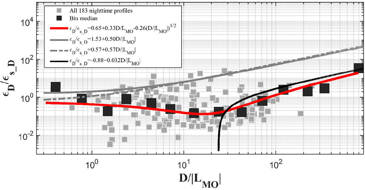
Figure 4 versus for all nighttime profiles (gray squares). The black squares denote the median values of 14 bins for all nighttime profiles, and they are fitted with Eqs. (15) and (17) as shown by the black and red solid lines, respectively. The gray line and gray dashed line denote the Eqs. (12) and (13), respectively.
We fitted these bin points (black squares) with Eq. (15), getting the coefficients A=-0.88 and B=0.032, as shown by the red line in Figure 4. The determination coefficient of this fitting is 0.03. It can only well represent the bin points when (When D/|LMO|< 20 the fitted line is negative). For comparison, Eqs. (12) and (13) were also shown with gray line and gray dashed line, respectively. These two lines could also not describe the present observation data, especially for the data when .
The linear combination for ϵD (Eq. (14) or (15)) could not well fit the present dataset to a certain extent, and much less does it reflect the transition character at . Moreover, when both wind stress and surface buoyancy flux are simultaneously driving turbulence in the mixed layer, their contributions to ϵ may be intercoupling, which implies that the linear combination of ϵs_D and for ϵD may not be an appropriate choice. To consider nonlinear coupling from wind stress and surface buoyancy flux, an extra nonlinear term was added to Eq. (14) to give
where A′ , B′ , and C′ are undetermined constants. Referring to the definition of LMO, Eq. (16) can be equivalently written as:
The dataset was fitted using Eq. (17), shown as the red solid line in Figure 4, with constants A′ = 0.65, B′ = 0.33, and C′ = -0.26. The determination coefficient is 0.31, much better than that of the linear fitting (Eq. (15)). Moreover, the fitting of Eq. (17) can well reflect the transition character of the data points at . It is worth noting that the coefficient C′ is negative, implying an opposite coupling effect of wind-induced current shear and buoyancy flux on turbulence kinetic energy dissipation rate. The mechanism behind this requires further research.
Although Eq. (17) could well fitted the present dataset collected from CINDY2011 in the tropical Indian Ocean, it is empirical and whether it can be extended to other sea areas needs further examination. However, this idea opens a window for further study of the interaction between the wind-driven stress and buoyancy fluxes in the mixed layer.
5 Summary
An observational dataset collected from CINDY2011 at the station (8°S, 80.5°E) in the tropical Indian Ocean was used to analyze statistically the vertical distribution of the TKE dissipation rate ϵ in the mixed layer. This dataset contains time series of high-resolution meteorological data, conventional hydrographic data, and turbulence microstructure data covering the whole mixed layer. The profiles of ϵ were statistically averaged using three methods. The arithmetic-mean method was significantly affected by individual outlier data and produced a more scattered ϵ profile. To examine the vertical distribution of ϵ in the mixed layer, ϵ was respectively scaled by the surface buoyancy flux and the TKE dissipation rate at the mixed-layer base ϵD for comparison. When the parameter ϵD was used, the dissipation rate ϵ showed similar vertical distributions in the mixed layer under different dynamic conditions (Figure 3D). This result indicates that ϵ follows a universal vertical structure within the mixed layer with ϵD as an intrinsic parameter. The parameterization of ϵD on shear-driven dissipation rate ϵs_D and the surface buoyancy flux was further quantitatively explored. The comparison indicated that a linear combination could better describe the variation trend and transition features of (Figure 4), in which the nonlinear term reflected the intercoupling characteristics between wind stress and buoyancy flux. The present study could be beneficial to our understanding of turbulence in the upper ocean boundary layer and might provide a reference for numerical modeling of the oceanic mixed layer.
Data availability statement
The original contributions presented in the study are included in the article/supplementary files. Further inquiries can be directed to the corresponding author.
Author contributions
SG and XC collected and analysed the field observation data and wrote the manuscript. SZ and YW provided advice and revised the manuscript. All authors contributed to the article and approved the submitted version.
Funding
This work was funded by National Key Research and Development Plan of China (2021YFC3101305, 2021YFC3101303), National Natural Science Foundation of China (91952106, 12172369), Southern Marine Science and Engineering Guangdong Laboratory (Guangzhou) (GML2019ZD0304, SMSEGL20SC01), and the research grants from State Key Laboratory of Tropical Oceanography (LTOZZ2001). The R/V MIRAI data were collected as part of the CINDY2011/DYNAMO project, which was sponsored by DOE, JAMSTEC, NASA, NOAA, NSF, and ONR. The CINDY2011 observational dataset used in this paper is available at https://www.jamstec.go.jp/cindy/obs/obs.html.
Conflict of interest
The authors declare that the research was conducted in the absence of any commercial or financial relationships that could be construed as a potential conflict of interest.
Publisher’s note
All claims expressed in this article are solely those of the authors and do not necessarily represent those of their affiliated organizations, or those of the publisher, the editors and the reviewers. Any product that may be evaluated in this article, or claim that may be made by its manufacturer, is not guaranteed or endorsed by the publisher.
References
Anis A., Moum J. N. (1994). Prescriptions for heat flux and entrainment rates in the upper ocean during convection. J. Physs. Oceanogr. 24 (10), 2142–2155. doi: 10.1175/1520-0485(1994)024<2142:PFHFAE>2.0.CO;2
Belcher S. E., Grant A. L. M., Hanley K. E., Baylor F-K, Van Roekel L., Sullivan P. P., et al. (2012). A global perspective on langmuir turbulence in the ocean surface boundary layer. Geophys. Res. Lett. 39 (18), L18605. doi: 10.1029/2012GL052932
Bluteau C. E., Jones N. L., Ivey G. (2016). Estimating turbulent dissipation from microstructure shear measurements using maximum likelihood spectral fitting over the inertial and viscous subranges. J. Atmos. Oceanic. Technol. 33, 713–722. doi: 10.1175/JTECH-D-15-0218.1
Brainerd K. E., Gregg M. C. (1993). Diurnal restratification and turbulence in the oceanic surface mixed layer: 1. observations. J. Geophys. Res-Oceans. 98 (C12), 22645–22656. doi: 10.1029/93JC02297
Brainerd K. E., Gregg M. C. (1995). Surface mixed and mixing layer depths. Deep. Sea. Res.-PT. I. 42 (9), 1521–1544. doi: 10.1016/0967-0637(95)00068-H
Callaghan A. H., Ward B., Vialard J. (2014). Influence of surface forcing on near-surface and mixing layer turbulence in the tropical Indian ocean. Deep-Sea. Res. PT. I. 94, 107–123. doi: 10.1016/j.dsr.2014.08.009
Chu P. C., Fan C. (2011). Maximum angle method for determining mixed layer depth from seaglider data. J. Oceanogr. 67 (2), 219–230. doi: 10.1007/s10872-011-0019-2
D'Asaro E. A. (2014). Turbulence in the upper-ocean mixed layer. Annu. Rev. Mar. Sci. 6, 101–115. doi: 10.1146/annurev-marine-010213-135138
de Boyer Montégut C., Madec G., Fischer A. S., Lazar A, Iudicone D. (2004). Mixed layer depth over the global ocean: An examination of profile data and a profile-based climatology. J. Geophys. Res-Oceans. 109 (C12), C12003. doi: 10.1029/2004JC002378
Edson J. B., Jampana V., Weller R. A., Bigorre S.P., Plueddemann A.J., Fairall C.W., et al. (2013). On the exchange of momentum over the open ocean. J. Physs. Oceanogr. 43 (8), 1589–1610. doi: 10.1175/JPO-D-12-0173.1
Esters L., Breivik Ø., Landwehr S., Doeschate ten A., Sutherland G., Christensen K.H., et al. (2018). Turbulence scaling comparisons in the ocean surface boundary layer. J. Geophys. Res-Oceans. 123 (3), 2172–2191. doi: 10.1002/2017JC013525
Esters L., Landwehr S., Sutherland G., Bell T.G., Christensen K.H., Saltzman E.S., et al. (2017). Parameterizing air-sea gas transfer velocity with dissipation. J. Geophys. Res-Oceans. 122 (4), 3041–3056. doi: 10.1002/2016JC012088
Evans D. G., Lucas N. S., Hemsley V., Frajka-Williams E., Naveira Garabato A. C., Martin A., et al. (2018). Annual cycle of turbulent dissipation estimated from seagliders. Geophys. Res. Lett. 45 (19), 10,560–10,569. doi: 10.1029/2018GL079966
Fairall C. W., Bradley E. F., Hare J. E., Grachev A.A., Edson J.B.. (2003). Bulk parameterization of air–sea fluxes: Updates and verification for the COARE algorithm. J. Climate 16 (4), 571–591. doi: 10.1175/1520-0442(2003)016<0571:BPOASF>2.0.CO;2
Fairall C. W., Bradley E. F., Rogers D. P., Edson J.B., Young G.S.. (1996). Bulk parameterization of air-sea fluxes for tropical ocean-global atmosphere coupled-ocean atmosphere response experiment. J. Geophys. Res-Oceans. 101 (C2), 3747–3764. doi: 10.1029/95JC03205
Ferrari R., Wunsch C. (2009). Ocean circulation kinetic energy: Reservoirs, sources, and sinks. Ann. Rev. Fluid. Mech. 41, 253–282. doi: 10.1146/annurev.fluid.40.111406.102139
Gemmrich J. R., Farmer D. M. (2004). Near-surface turbulence in the presence of breaking waves. J. Physs. Oceanogr. 34 (5), 1067–1086. doi: 10.1175/1520-0485(2004)034<1067:NTITPO>2.0.CO;2
Grachev A. A., Fairall C. W. (1997). Dependence of the monin–obukhov stability parameter on the bulk Richardson number over the ocean. J. Appl. Meteorol. 36 (4), 406–414. doi: 10.1175/1520-0450(1997)036<0406:DOTMOS>2.0.CO;2
Holte J., Talley L. (2009). A new algorithm for finding mixed layer depths with applications to argo data and subantarctic mode water formation. J. Atmos. Ocean. Tech. 26 (9), 1920–1939. doi: 10.1175/2009JTECHO543.1
Huang P. Q., Lu Y. Z., Zhou S. Q. (2018). An objective method for determining ocean mixed layer depth with applications to WOCE data. J. Atmos. Ocean. Tech. 35 (3), 441–458. doi: 10.1175/JTECH-D-17-0104.1
Imberger J. (1985). The diurnal mixed layer 1. Limnol. Oceanogr. 30 (4), 737–770. doi: 10.4319/lo.1985.30.4.0737
Jones I. S., Toba Y. (Eds.) (2001). Wind stress over the ocean (Cambridge, England, GB: Cambridge University Press).
Kantha L. H., Clayson C. A. (2000). Small scale processes in geophysical fluid flows (San Francisco, California, USA: Elsevier).
Kostov Y., Armour K. C., Marshall J. (2014). Impact of the Atlantic meridional overturning circulation on ocean heat storage and transient climate change. Geophys. Res. Lett. 41 (6), 2108–2116. doi: 10.1002/2013GL058998
Lombardo C. P., Gregg M. C. (1989). Similarity scaling of viscous and thermal dissipation in a convecting surface boundary layer. J. Geophys. Res-Oceans. 94 (C5), 6273–6284. doi: 10.1029/JC094iC05p06273
Lorbacher K., Dommenget D., Niiler P. P., Köhl A.. (2006). Ocean mixed layer depth: A subsurface proxy of ocean-atmosphere variability. J. Geophys. Res-Oceans. 111 (C7), C07010. doi: 10.1029/2003JC002157
Lozovatsky I., Figueroa M., Roget E., Fernando H. J. S., Shapovalov S.. (2005). Observations and scaling of the upper mixed layer in the north Atlantic. J. Geophys. Res-Oceans. 110 (C5), C05013. doi: 10.1029/2004JC002708
Macdonald A. M., Wunsch C. (1996). An estimate of global ocean circulation and heat fluxes. Nature 382 (6590), 436–439. doi: 10.1038/382436a0
Meredith M., Garabato A. N. (Eds.) (2021). Ocean mixing: Drivers, mechanisms and impacts (London, England, GB, Elsevier).
Monin A. S., Yaglom A. M. (1971). Statistical fluid mechanics Vol. Vol. 1 (Cambridge: MIT Press), 766–769.
Moulin A. J., Moum J. N., Shroyer E. L. (2018). Evolution of turbulence in the diurnal warm layer. J. Physs. Oceanogr. 48 (2), 383–396. doi: 10.1175/JPO-D-17-0170.1
Moum J. N., Gregg M. C., Lien R. C., Carr M.E.. (1995). Comparison of turbulence kinetic energy dissipation rate estimates from two ocean microstructure profilers. J. Atmos. Ocean. Tech. 12 (2), 346–366. doi: 10.1175/1520-0426(1995)012<0346:COTKED>2.0.CO;2
Moum J. N., Rippeth T. P. (2009). Do observations adequately resolve the natural variability of oceanic turbulence? J. Mar. Syst. 77 (4), 409–417. doi: 10.1016/j.jmarsys.2008.10.013
Oakey N. S., Elliott J. A. (1982). Dissipation within the surface mixed layer. J. Physs. Oceanogr. 12 (2), 171–185. doi: 10.1175/1520-0485(1982)012<0171:DWTSML>2.0.CO;2
Pellichero V., Sallée J. B., Schmidtko S., Roquet F., Charrassin J.-B.. (2017). The ocean mixed layer under southern ocean sea-ice: Seasonal cycle and forcing. J. Geophys. Res-Oceans. 122 (2), 1608–1633. doi: 10.1002/2016JC011970
Qiu C., Cui Y., Ren J., Wang Q., Huo D., Wu J., et al. (2016). Characteristics of the surface mixed layer depths in the northern south China Sea in spring. J. Oceanogr. 72 (4), 567–576. doi: 10.1007/s10872-016-0351-7
Qiu C., Huo D., Liu C., Cui Y., Su D., Wu J., et al. (2019). Upper vertical structures and mixed layer depth in the shelf of the northern south China Sea. Cont. Shelf. Res. 174, 26–34. doi: 10.1016/j.csr.2019.01.004
Sabine C. L., Feely R. A., Gruber N., Key R.M., Lee K., Bullister J.L., et al. (2004). The oceanic sink for anthropogenic CO2. Science 305 (5682), 367–371. doi: 10.1126/science.10974
Seiki A., Katsumata M., Horii T., Hasegawa T., Richards K.J., Yoneyama K., et al. (2013). Abrupt cooling associated with the oceanic rossby wave and lateral advection during CINDY2011. J. Geophys. Res-Oceans. 118 (10), 5523–5535. doi: 10.1002/jgrc.20381
Shay T. J., Gregg M. C. (1986). Convectively driven turbulent mixing in the upper ocean. J. Physs. Oceanogr. 16 (11), 1777–1798. doi: 10.1175/1520-0485(1986)016<1777:CDTMIT>2.0.CO;2
Tedford E. W., MacIntyre S., Miller S. D., Czikowsky M. J.. (2014). Similarity scaling of turbulence in a temperate lake during fall cooling. J. Geophys. Res-Oceans. 119 (8), 4689–4713. doi: 10.1002/2014JC010135
Thompson E. J., Moum J. N., Fairall C. W., Rutledge S.A.. (2019). Wind limits on rain layers and diurnal warm layers. J. Geophys. Res-Oceans. 124 (2), 897–924. doi: 10.1029/2018JC014130
Thomson R. E., Fine I. V. (2003). Estimating mixed layer depth from oceanic profile data. J. Atmos. Ocean. Tech. 20 (2), 319–329. doi: 10.1175/1520-0426(2003)020<0319:EMLDFO>2.0.CO;2
Wain D. J., Lilly J. M., Callaghan A. H., Yashayaev I., Ward B.. (2015). A breaking internal wave in the surface ocean boundary layer. J. Geophys. Res-Oceans. 120 (6), 4151–4161. doi: 10.1002/2014JC010416
Wolk F., Yamazaki H., Seuront L., Lueck R.G.. (2002). A new free-fall profiler for measuring biophysical microstructure. J. Atmos. Ocean. Tech. 19 (5), 780–793. doi: 10.1175/1520-0426(2002)019<0780:ANFFPF>2.0.CO;2
Wunsch C., Ferrari R. (2004). Vertical mixing, energy, and the general circulation of the oceans. Ann. Rev. Fluid. Mech. 36, 281–314. doi: 10.1146/annurev.fluid.36.050802.122121
Yoneyama K., Zhang C., Long C. N. (2013). Tracking pulses of the madden–Julian oscillation. B. Am. Meteorol. Soc 94 (12), 1871–1891. doi: 10.1175/BAMS-D-12-00157.1
Keywords: turbulent mixing, dissipation rate, tropical indian ocean, mixed layer, similarity
Citation: Cen X-R, Guo S-X, Wang Y and Zhou S-Q (2022) Similarity of the turbulent kinetic energy dissipation rate distribution in the upper mixed layer of the tropical Indian Ocean. Front. Mar. Sci. 9:1035135. doi: 10.3389/fmars.2022.1035135
Received: 02 September 2022; Accepted: 17 October 2022;
Published: 03 November 2022.
Edited by:
François G. Schmitt, UMR8187 Laboratoire d'océanologie et de géosciences (LOG), FranceCopyright © 2022 Cen, Guo, Wang and Zhou. This is an open-access article distributed under the terms of the Creative Commons Attribution License (CC BY). The use, distribution or reproduction in other forums is permitted, provided the original author(s) and the copyright owner(s) are credited and that the original publication in this journal is cited, in accordance with accepted academic practice. No use, distribution or reproduction is permitted which does not comply with these terms.
*Correspondence: Shuang-Xi Guo, c3hndW9Ac2NzaW8uYWMuY24=