Deep blue artificial intelligence for knowledge discovery of the intermediate ocean

Oceans at a depth ranging from ~100 to ~1000-m (defined as the intermediate water here), though poorly understood compared to the sea surface, is a critical layer of the Earth system where many important oceanographic processes take place. Advances in ocean observation and computer technology have allowed ocean science to enter the era of big data (to be precise, big data for the surface layer, small data for the bottom layer, and the intermediate layer sits in between) and greatly promoted our understanding of near-surface ocean phenomena. During the past few decades, however, the intermediate ocean is also undergoing profound changes because of global warming, the research and prediction of which are of intensive concern. Due to the lack of three-dimensional ocean theories and field observations, how to remotely sense the intermediate ocean from space becomes a very attractive but challenging scientific issue. With the rapid development of the next generation of information technology, artificial intelligence (AI) has built a new bridge from data science to marine science (called Deep Blue AI, DBAI), which acts as a powerful weapon to extend the paradigm of modern oceanography in the era of the metaverse. This review first introduces the basic prior knowledge of water movement in the ~100 m ocean and vertical stratification within the ~1000-m depths as well as the data resources provided by satellite remote sensing, field observation, and model reanalysis for DBAI. Then, three universal DBAI methodologies, namely, associative statistical, physically informed, and mathematically driven neural networks, are elucidated in the context of intermediate ocean remote sensing. Finally, the unique advantages and potentials of DBAI in data mining and knowledge discovery are demonstrated in a top-down way of “surface-to-interior” via several typical examples in physical and biological oceanography.

1. Introduction

Since the advent of ocean remote sensing technology, the understanding of surface or near-surface ocean phenomena has been improving. Nevertheless, the phenomena mined from satellite remote sensing data are only the tip of the iceberg because that ocean is a huge body of water that is thousands of deep, the maximum depth of which can reach 10,000 meters. Consequently, the comprehensive recognition of the deep blue ocean from the outside to the inside has always been a challenging scientific issue.

The hectometer-scale ocean contains abundant dynamic and ecological processes from turbulence to circulation, from waves to tides, and from oxygen minimum zones to subsurface chlorophyll maximum (SCM), whereas the kilometer-scale ocean is relatively “calm” and significant stratification acts as a barrier to the exchange of matter and energy between the upper and lower waters. However, slight changes in the thermohaline and circulation structures of the kilometer-scale ocean are reminders of climate change on the decadal scale. Before the turn of this century, increasingly mature oceanographic theories and the continuous accumulation of field and remote sensing data have been building the foundation of modern ocean science with the cognition of near-surface ocean phenomena and laws.

Compared with the near-surface layer, the intermediate ocean at the depth of ~100 to ~1000 meters is facing difficulties, such as the lack of corresponding theories and insufficient three-dimensional observation, which are the main factors restricting the further development of marine science (Meng and Yan, 2022). In the 21st century, the in situ observation and model reanalysis technologies represented by the Array for Real-time Geostrophic Oceanography (Argo) have developed rapidly, providing unprecedented high-quality data sources for intermediate ocean research.

Meanwhile, prevalent AI technology gradually developed a new branch, termed DBAI, with a unique data-driven advantage of knowledge discovery. DBAI provides the opportunity to accelerate the recognition process of the intermediate ocean, making up for the deficiency of the existing oceanographic theoretical system. In recent years, DBAI technology, in collaboration with basic ocean theory and ocean big data (Li et al., 2020), has made preliminary achievements in internal wave (IW) inversion, stratification spatio-temporal variation and prediction, eddy identification and trajectory prediction, El Nino and Southern Oscillation prediction and other ocean scientific issues Ham et al. (2019); Zhang et al. (2022). Nevertheless, it is undeniable that AI-aided remote sensing of the intermediate ocean is still in its infancy, and the challenges lie in the unclear physical mechanism, insufficient profile data, and the low generalization DBAI. The gap between remote sensing data and knowledge can be filled with the construction of DBAIwith strong knowledge discovery and physical interpretability, thus promoting major discoveries and theoretical innovations in intermediate marine science.

1.1. Water motion in ~100-m ocean

As a large-scale geophysical fluid system, the ocean is forced by celestial bodies, atmosphere, earth rotation, and the system itself, so that the upper water movement covers a very broad three-dimensional space-time scale. Generally speaking, the larger the spatial scale of water movement is, the longer the period is, and the deeper the ocean water layer is affected. As illustrated in Figure 1A.

FIGURE 1

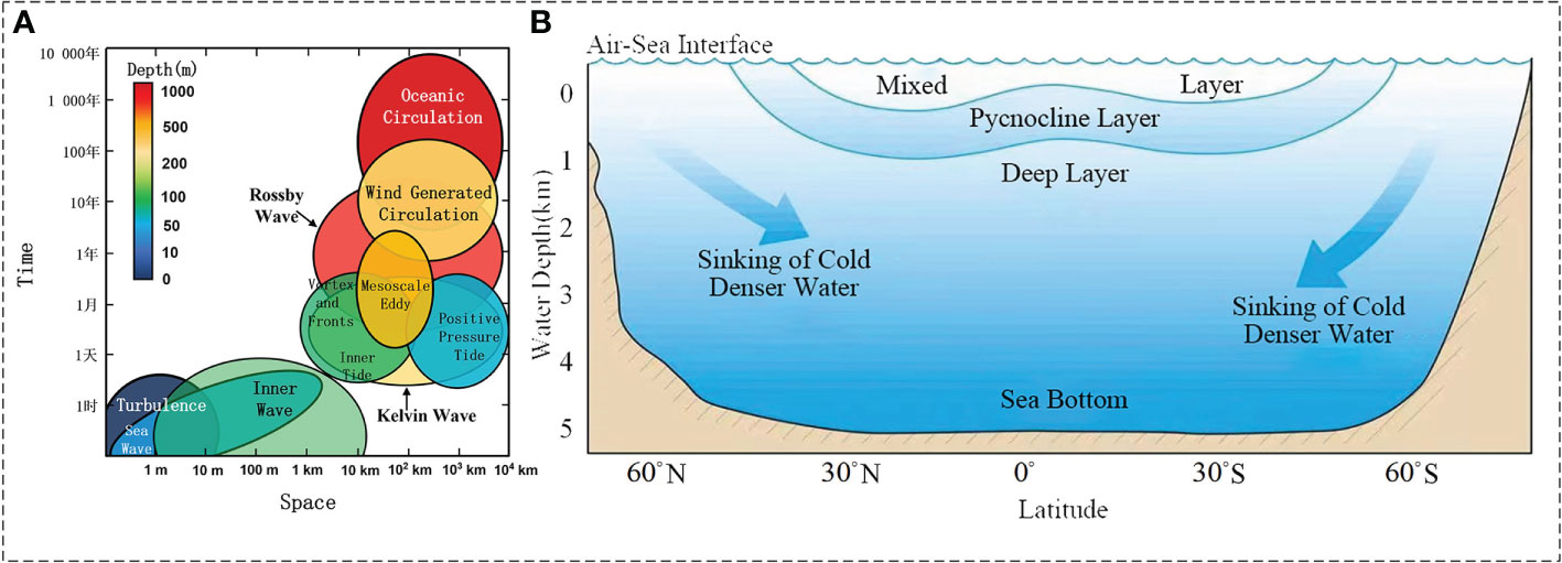
Figure 1 Water motion and vertical stratification of the intermediate ocean. (A) The time scale, spatial scale and depth of various types of motions. (B) Vertical stratification.

Ocean motions can be broadly divided into turbulence, wave, and flow. On the small scale (millimeter magnitude) and high-frequency motion spectrum, the velocity (magnitude and direction) of any particle in seawater varies in a disordered manner, which is collectively referred to as turbulence. Turbulence mainly occurs at the surface of the ocean and plays an important role in the multiscale energy cascade of fluids. Its maintenance depends on the external energy supply (wave breaking is the most typical source) and follows fluid dynamics equations (such as Navier–Stokes equations).

The oceanic wave phenomena mainly include waves, tides, IWs, large-scale Rossby waves, and Kelvin waves. The effective wave height and tidal water level change are usually within 10 meters, whereas the surge can reach tens of meters in extreme weather, and the offshore tidal power can even reach the bottom. In addition, the tides have the horizontal scale of a kilometer and are potentially coupled with large-scale Rossby and Kelvin waves (sea surface height anomalies of 10 cm and vertical scales of thousands of meters). Ocean current is defined as a large-scale, relatively stable flow of seawater driven by wind stress and density differences. The core depth of ocean circulation is usually several hundred meters, and the deep compensation undercurrent can reach the depth of kilometers. It is crucial in the composition of the global ocean environment and climate regulation.

1.2. Vertical stratification of the ~1000-m ocean

In addition to the flow and fluctuation in the horizontal direction, the ocean also has typical stratification characteristics in the vertical direction. According to the range of air–sea interaction and the vertical gradient of thermohaline parameters, the ocean water can be divided into the air–sea interface, mixed layer, thermocline, and deep layer from top to bottom (Sprintall and Cronin, 2009) as illustrated in Figure 1B.

Among them, the air–sea interface is related to the momentum, heat, and gas exchange rate between the ocean and the atmosphere, which has become the key problem of climate change and its prediction. Turbulent mixing caused by dynamic effects (wind, wave, current, etc.) and convective mixing caused by thermal effects (evaporation, cooling, densification, etc.) at the air–sea interface makes the upper ocean form a water layer with nearly uniform temperature, salinity, and density field, that is, the mixed layer, which contributes to the heat balance, water cycle, and carbon cycle of the earth system. Meanwhile, climate and large-scale atmospheric circulation changes have direct and important effects. At the lower boundary of the mixing layer, the water layer with rapid changes in temperature, salinity, and density is called the marine thermocline, which is divided into the seasonal and main thermocline. The existence of the thermocline hinders the exchange of heat, oxygen, carbon, and nutrients between the upper and lower water bodies, and its interannual and interdecadal changes are reflected in the climate system and the Marine ecosystem. Below the thermocline is uniform deep water with basically stable temperature, salinity, and density characteristics.

From the perspective of time scale, the air–sea interaction at the interface takes place at any time, the mixed layer and the seasonal thermocline have synoptic and seasonal scales, and the main thermocline and deep water change slowly on decadal and climatic scales. From the perspective of spatial scale, the mixed layer is usually fewer than 100 meters in the low latitude sea area and can be as deep as the main thermocline in the middle latitude. The main thermocline is about 300 m in the low latitude and 700~800 m in the middle latitude. At the high latitude, the mixed layer and the main thermocline gradually rise until the stratification of subpolar water disappears. In general, the air–sea interface and mixing layer are the most active areas of ocean mixing, which are directly affected by the weather system. The stratification structure and thermohaline distribution of the thermohaline circulation are controlled by the seawater subsidence and have climatic-scale characteristics. Therefore, the distribution of temperature, salinity, and density fields in the vertical direction in the low-latitude sea area reflects the radial spatial distribution characteristics of the ocean surface to a certain extent (Trujillo and Thurman, 2011).

1.3. DBAI-aided remote sensing of the intermediate ocean

As an interdisciplinary science based on observation and experiment, marine science, which is characterized by data-intensive and technology integration and linked by water bodies, has experienced a development process from theoretical traction to technology-driven and then to data-driven. Specifically, the model-driven method is to achieve theoretical analytical solutions by modeling problems, just as Western medicine treats patients based on the diagnosis. Data-driven methods search for the approximate optimal solutions by fitting the model to the data, just like “look, hear, question, and feel the pulse” in traditional Chinese medicine, which is guided by traditional Chinese philosophy to carry out “characteristic engineering” with dialectical unity. Western medicine takes Western philosophy as a “mathematical model” to solve the main contradiction quickly and efficiently. “AI for science” is listed as an important trend, indicating that “AI can become a new production tool for scientists and promote the new paradigm change in scientific research” (Appenzeller, 2021). As a cutting-edge technology in the integration of marine and data science, DBAI has the function of “model + data” driving and complementing each other in the way of “integration of traditional Chinese and Western medicine.”

This review paper puts forward the viewpoint of philosophy and scientific conception of DBAI for the first time as shown in Figure 2. Although satellite ocean remote sensing is the main approach to observing surface and subsurface ocean phenomena from the “external” perspective, it cannot directly perceive the “internal” process of the intermediate ocean. Benefiting from the in situ observation represented by Argo buoys, the vertical profiles compensate for the existing deficiencies of satellite ocean remote sensing with high accuracy. However, it cannot achieve extensive coverage at the same time. Therefore, it is crucial to combine the remote sensing data with the in situ data; DBAI technology is highly promising for playing such a role.

FIGURE 2

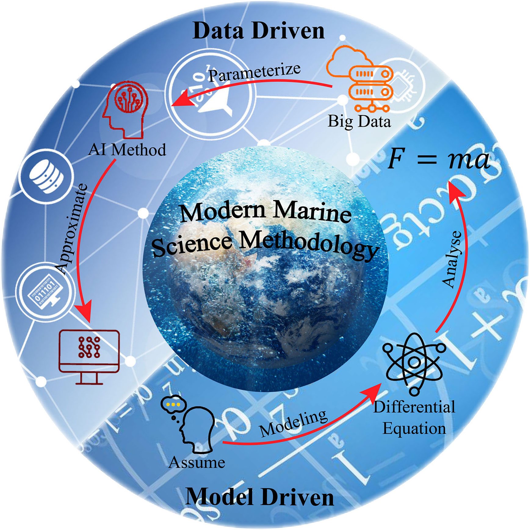
Figure 2 Philosophy and scientific conception of DBAI, model-driven and data-driven methods supplement each other, just as Western and Chinese medicine complement each other.

The remainder of this review paper proceeds as follows. Section 2 describes the ocean observations regarding the satellite remote sensing in the ~100-m ocean and in situ observations in the ~1000-m ocean. In section 3, the DBAI methodology is introduced in detail and contains associative statistical, physically informed, and mathematically driven neural networks. Section 4 demonstrates the knowledge discovery with DBAI. Finally, some remarks conclude in Section 5.

2. Observations

Observations are highly significant in oceanographic progress, and DBAI is increasingly being considered as a tool to exchange ocean knowledge and observational data for the intermediate ocean as well as bring together model- and data-driven methods, facilitating conventional tasks better and faster. The observations of the intermediate ocean can be divided into satellite remote sensing in the ~100-m ocean and in situ observations in the ~1000-m ocean.

2.1. Satellite remote sensing in the ~100-m ocean

Oceanic remote sensing, as one of the key technologies to promote the development of marine science, has acquired ocean color, dynamics, and environmental parameters with its comprehensive advantages of all-weather, quasi-real-time, large range, high precision, and long-time sequence over the past 50 years. It has fundamentally enhanced our profound understanding of near-surface ocean phenomena and processes such as ocean primary productivity, sea level change, air–sea flux, and ocean circulation and improved the traditional paradigm of global ocean observation and scientific research.

However, current satellite ocean remote sensing is essentially a two-dimensional sea surface remote sensing. As an active optical remote sensing method, light detection and ranging (LiDAR) has the combined technical advantages of all-day range resolution and large penetration depth (more than three times that of passive remote sensing). Moreover, LiDAR can achieve remote sensing at night, in polar regions, and even in cloudy conditions. At present, it is the only known detection method that is expected to realize underwater three-dimensional remote sensing and is also the international frontier in the field of ocean optics and ocean water color remote sensing (Hostetler et al., 2018). Furthermore, LiDAR is widely applied in marine bio-optics, shallow sea topography, fish detection, polar ecology, and upper ocean dynamic processes (IWs, mixed layers, turbulence, foam, etc.). In other words, a new interdisciplinary technology field that is marine LiDAR detection technology has been gradually constructed (Churnside, 2013).

Although the spaceborne marine LiDAR is still in the blank stage, the successfully launched spaceborne atmospheric LiDAR (CALIOP) and terrestrial LiDAR (ICESat-2) have shown good advantages and potential in the preliminary application of ecological oceanography (Behrenfeld et al., 2013; Behrenfeld et al., 2017; Behrenfeld et al., 2019; Lu et al., 2020). With the successive planning and implementation of the NASA PACE mission (Werdell et al., 2019), ESA MESCAL mission (Chepfer et al., 2018), and Guanlan mission (Chen et al., 2019) of China Ocean National Laboratory Qingdao, Spaceborne marine LiDAR with multiband (blue-green wavelength), meter-level resolution and multisystem (hyperspectral, fluorescence, polarization, etc.) observation capability will become a reality. The concept design of observation at ~100 m depth can be seen in Figure 3. Further combined with passive ocean color remote sensing and in situ biogeochemical buoys (Biogeochemical Argo, BGC-ARGO) and other observation means, it is expected to achieve the three-dimensional detection and high-precision inversion of bio-optical and physical parameters in four-dimensional space time within the ~100-m depth of the global ocean for the first time (Chen et al., 2021b). For a more intuitive understanding of the abovementioned spaceborne sensor, the characteristics of these satellite sensors are collected and summarized in Table 1 (Amani et al., 2021; Amani et al., 2022a; Amani et al., 2022b; Amani et al., 2022c).

FIGURE 3

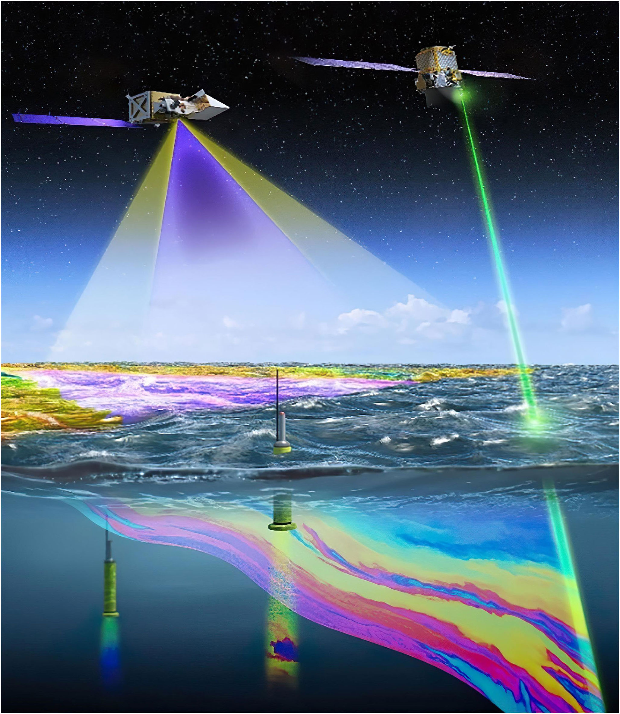
Figure 3 Concept design of the integration of active and passive remote sensing and field joint observation at ~100-m depth.

TABLE 1

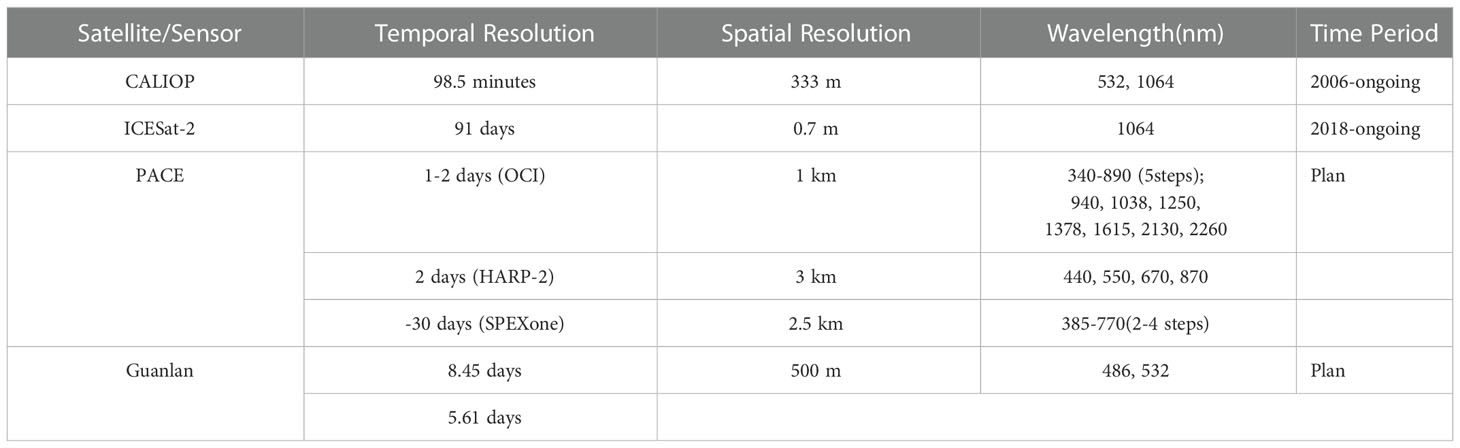
Table 1 The characteristics of described spaceborne satellite and mission.

2.2. In situ observations in the ~1000-m ocean

The ~1000-m ocean is usually studied with the help of in situ observations and reanalysis data. Before the 21st century, in situ profile observation typically comprised ship-based and mooring buoy array but was challenged in terms of the low coverage rate of spatiotemporal data, large deviation, and high observation cost. In the 1990s, with the intensification of global climate change and the prominent role of the ocean, the systematic absence of global ocean profile observation data posed great challenges to climate change research (Johnson et al., 2022).

In this context, the Argo program, which aims at the real-time acquisition of global ocean thermohaline data at in the upper 2000 m, was implemented. Up to now, it has provided more than 95% of global thermohaline profile data (Riser et al., 2016), bringing profound changes to intermediate marine scientific research. In the early 21st century, mobile observation and sensor technologies were further developed (Morel and Berthon, 1989). Physical, biological, and chemical sensors with miniature and low power consumption were successfully developed, and BGC-Argo buoys proceeded, providing a broader data basis for exploring the coupling of ocean physics and biogeochemistry. Around 2012, the United States, France, and other countries successively joined the Deep-sea Argo (Deep-Argo) program, planning to build a deep-sea Argo observation network measuring depths up to 6000 m to promote the Argo program to enter the era of all-sea, all-depth, and multidisciplinary ocean observation. Figure 4 illustrates the Labrador Sea temperature profile based on Argo measurement.

FIGURE 4

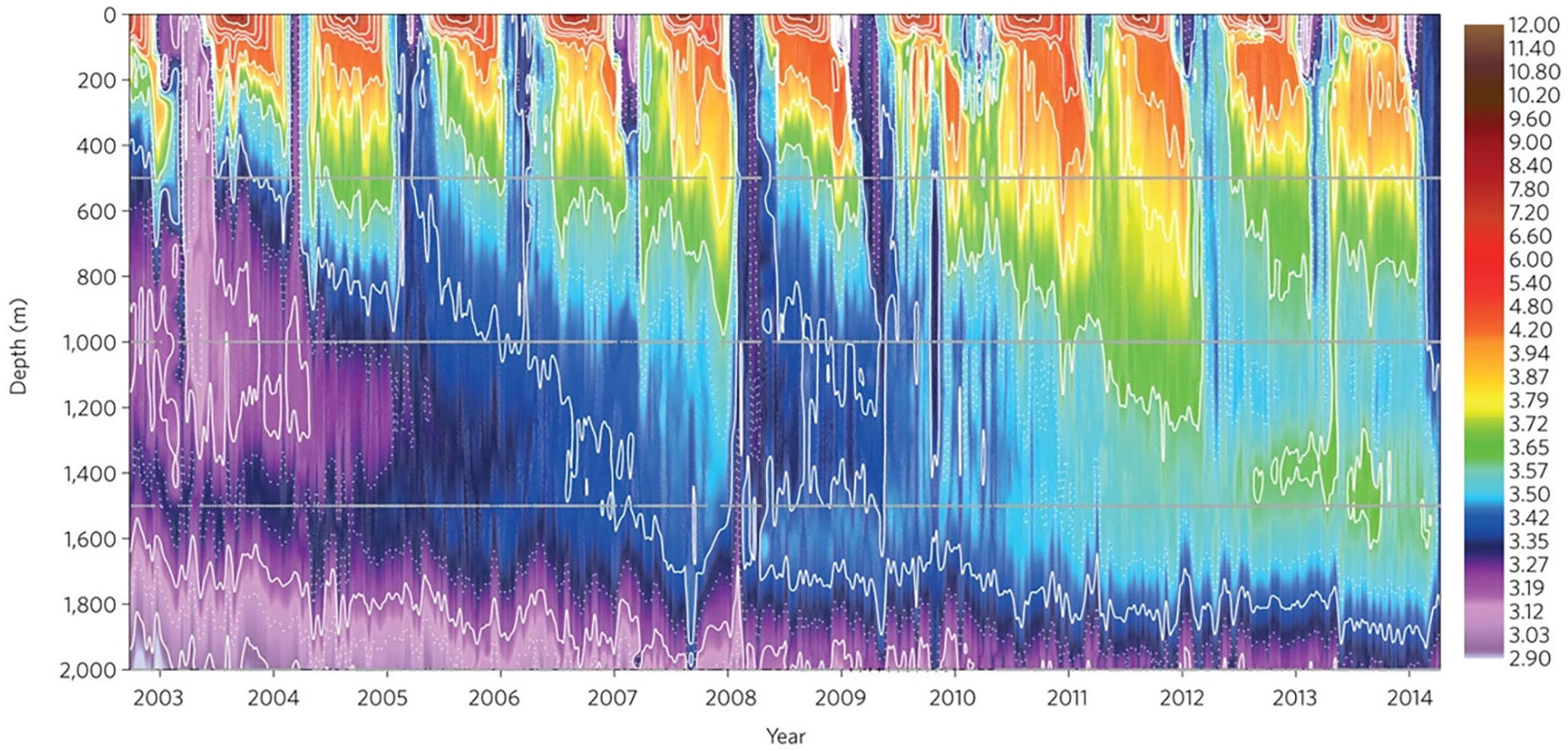
Figure 4 Labrador Sea temperature profile obtained from in situ Argo observations.

Additionally, with the rapid development of ocean observation technology and the significant improvement of computer performance, the development and application of high spatiotemporal resolution, full-sea depth, numerical simulation products based on the earth fluid dynamics theory and the assimilation of multisource observation data have significantly improved the accuracy of model prediction results. Ocean model and climate state observation data products, such as the hybrid coordinate ocean model (HYCOM), global ocean circulation model data set, and world ocean atlas (WOA) global Ocean grid climate state data set, have emerged. Including temperature, salinity, flow field, chlorophyll, inorganic salt, and other multilayer parameter information related to marine thermal, marine dynamics and biogeochemistry, and other fields, provides another foundational data source for intermediate and even deep ocean scientific research. In recent years, in situ imagery acquired by underwater imagers has been major ancillary data in marine research. However, different from the remote sensing images, the complicated situations of the marine environment highlight the uneven distribution of data quality in in situ images (Jian et al., 2021). In situ images enhanced, denoised, or saliently extracted by specific algorithms provide a reliable data source for full ocean-depth scientific research (Jian et al., 2018; Jian et al., 2019).

3. DBAI methodology

DBAI methodology mines the essence of phenomena and reveals the laws behind them, starting from the data dimension and taking scientific calculation as the core. As the key component, the neural network (Cozman, 2021) develops from shallow to deep (Lecun et al., 1998; Ronneberger et al., 2015) and has undergone three stages: associative statistical, physically informed, and mathematically driven. The associative statistical neural networks can extract the information of data space, mine the explicit laws contained in the data, and realize basic knowledge discovery. Physically informed neural networks (PINNs) (Wright et al., 2022) embed disciplined prior knowledge or theory into the network, extract potential knowledge rules from data, improve operation efficiency, and prevent “low-level fallacy.” By building a bridge between the traceable mathematical model and scientific knowledge, the mathematically driven neural networks give full play to the excellent performance of the deep neural network in chaotic or extremely complex mass data and achieve valuable knowledge, accelerating scientific discovery and enabling interpretable results. The overall architecture of DBAI is illustrated in Figure 5. The data obtained by satellite remote sensing and in situ observations allow for surface-to-interior profiling of ocean phenomena. AI technology bridges the semantic gap between the two data sources, efficiently coupling remote sensing data, which has the external advantage, with in situ data, which has an internal character. This coupled paradigm makes DBAI technology, which incorporates mathematically driven, physically informed, and associative statistical, a new engine for knowledge discovery in marine science.

FIGURE 5

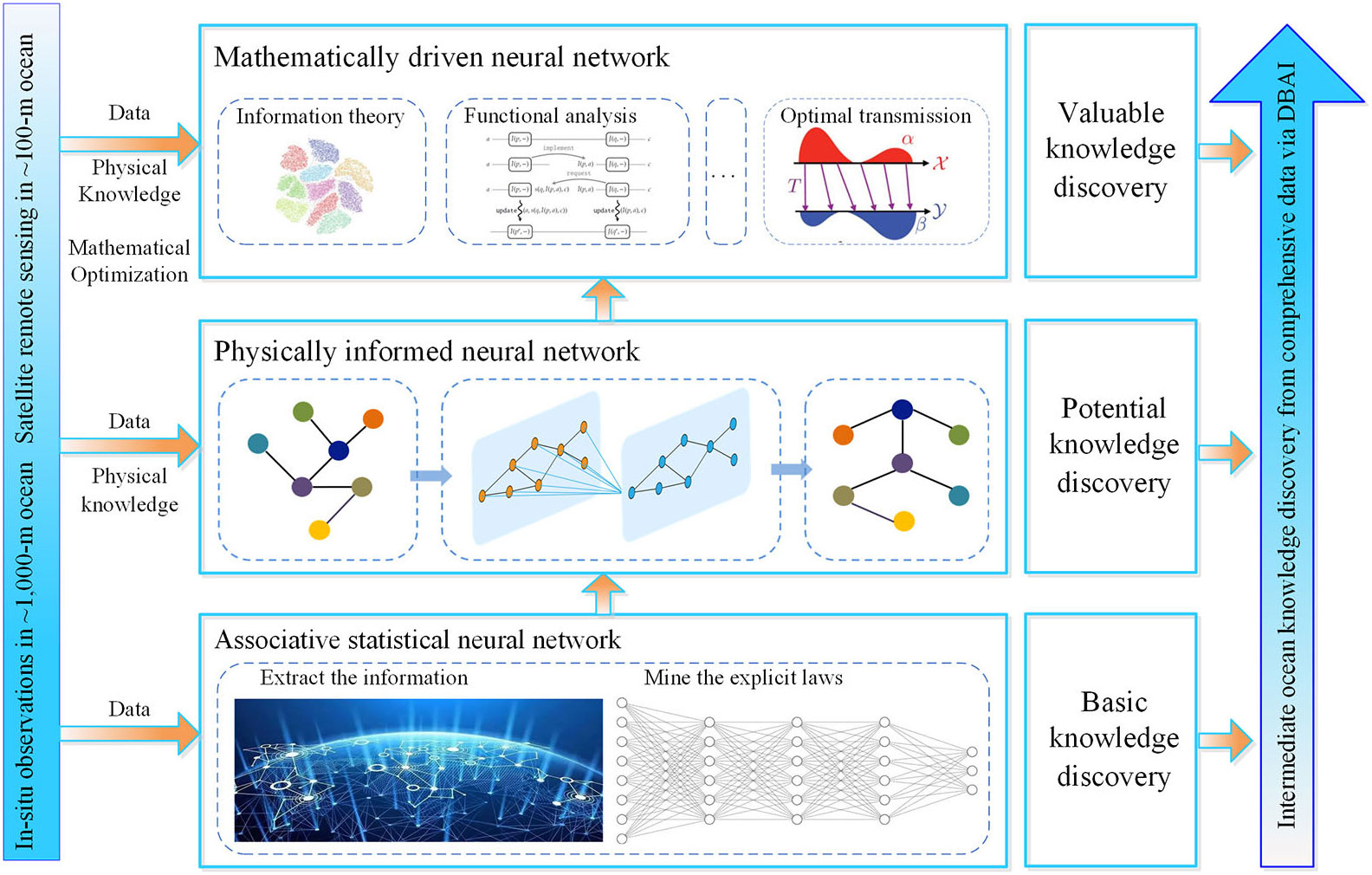
Figure 5 Overall architecture of DBAI. The core of DBAI is the associative statistical, physically informed, mathematically driven neural networks.

3.1. Associative statistical neural network

The basic method or function of the DBAI methodology is to perform correlation statistics in the data ocean, achieving initial and explicit information mining and knowledge discovery. Data is the fuel of the AI method; the construction methods of the neural network vary with different data features. For example, the image data and rasterized products in remote sensing are general data types, which can be obtained with special equipment. With the development of computer vision (Simonyan and Zisserman, 2015; Huang et al., 2017; Chen et al., 2018), neural networks can mine the local features of objects in these data. Thus, most of the explorative DBAI research is based on Euclidean data to construct convolutional neural networks (He et al., 2017) and then achieves the correlation statistics of data information. In terms of DBAI architecture, the basic building blocks are convolution neural network, recurrent neural network and its extended network, such as the LSTM unit, as shown in Figure 6. The convolution neural network, which is depicted in Figure 6A, provides a new mathematics tool for researching grid data (Goodfellow et al., 2014; He et al., 2016). Furthermore, with continuous iterative updating, the recurrent neural networks, the structures of which are shown in Figure 6B, C, can explore the timeseries features and context information from long-time series data.

FIGURE 6

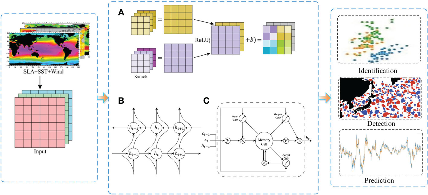
Figure 6 Associative statistical neural network schematic; the basic building blocks include (A) convolutional neural network, (B) recurrent neural network feedforward process, and (C) LSTM structure.

As for sensory data, the sea surface temperature, sea surface height, and sea level anomaly (SLA) have time series features that can extract the parameters of the feature for change of temperature and height with time lapse adopting the recurrent neural networks. Then, the model summarizes the overall pattern of the data to predict the future trend. Therefore, associative statistical neural networks are becoming one of the basic methodologies for researchers to detect and predict oceanic phenomena and grasp their patterns. Table 2 displays some research for constructing the neural network based on Euclidean data in marine science from 2018 to now. The application direction and publication time illustrate that DBAI is the environment of mass innovation that can continue to develop.

TABLE 2

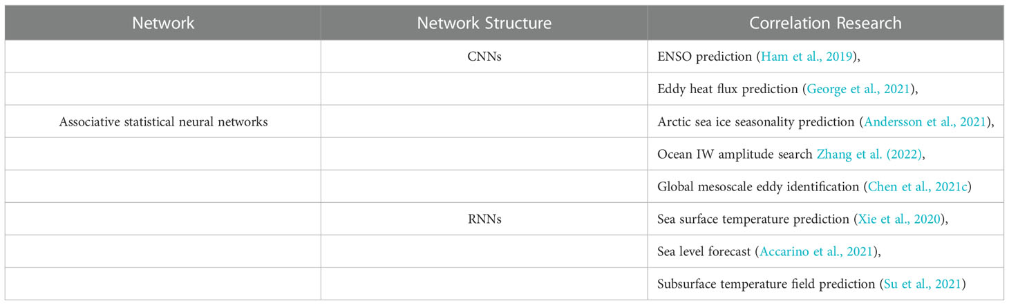
Table 2 Partially associative statistical neural networks for mid-level ocean remote sensing.

As previously identified, the data is the beginning of the associative statistical neural networks, which are based on the classification of the data and characteristics of the task to design the network structure. However, in scientific research, it is key to incorporate physical theory into neural networks to enable even higher accuracy.

3.2. Physically informed neural network

To exploit the efficiency of the neural network, the PINN is proposed by Raissi et al. (2019). PINNs follow the specific objective laws of physics described by nonlinear differential equations, which is a deep learning method that can solve scientific problems (Nakajima et al., 2021). PINNs are a pioneering technology that provides PDE with a new numerical solver. According to the guide method, it can be divided into observation, induction, and learning bias (Karniadakis et al., 2021), which is shown in Figure 7.

FIGURE 7

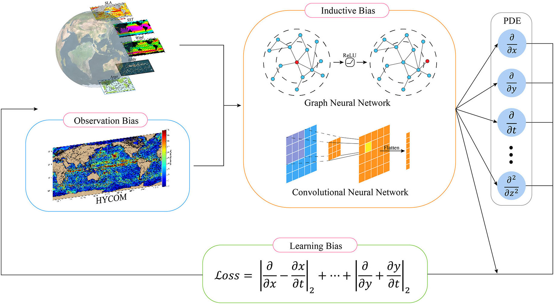
Figure 7 Prior knowledge-embedding mechanism for PINNs.

The observation bias is designed for the data input stage because the data can reflect the underlying physics. For example, with the universal gravitation $\text{F}=\frac{GMm}{r^2}$, Burges function $\frac{\partial u}{\partial t}+u\frac{\partial u}{\partial x}=v\frac{{\partial }^{2}u}{\partial x^2}$, and Hamiton systems $\frac{\partial H}{\partial p}=\frac{\partial p}{\partial t},\frac{\partial H}{\partial q}=-\frac{\partial q}{\partial t}$, neural networks can learn the physical structure, functions, vector fields, etc., from these physical principles, achieving being physically informed.

Furthermore, in the model-learning process, we expect that some specific features can be prioritized. Thus, the induction bias is introduced in the neural network, which utilizes the universal rules in the physical world to constrain the model. Normally, in the construction process of the network, the induction bias is designed for a neural operator that makes the computational process follow the physical law, for example, the translational and spatial invariance in CNNs and graph embedding computation in graph neural networks.

The learning bias is different from the above guided method; it focuses on the backward neural network. In other words, a dedicated loss function is designed for the model to calculate the error. Suppose that a problem satisfies a constraint, and the output of the network can transform into a mapping of solutions. For instance, the hamiltonian system (Greydanus et al., 2019) description formula transforms into a form of residuals, such as (1).

$\begin{array}{ll}\frac{\partial H}{\partial p}-\frac{\partial p}{\partial t}=0,\frac{\partial H}{\partial q}+\frac{\partial q}{\partial t}=0& (1)\end{array}$

In this function, p denotes coordinate and q is momentum. According to the residual function, the loss function can be designed as Equation (2).

$\begin{array}{ll}L={\left|\frac{\partial H}{\partial p}-\frac{\partial p}{\partial t}\right|}_2+{\left|\frac{\partial H}{\partial q}+\frac{\partial q}{\partial t}\right|}_2& (2)\end{array}$

The learning bias prompts the trained neural network to conform to the theory that is expressed by differential or partial differential equations. That improves the confidence and prediction accuracy of neural networks significantly. Table 3 enumerates part of the research that PINNs applies in marine science and lists the bias method.

TABLE 3

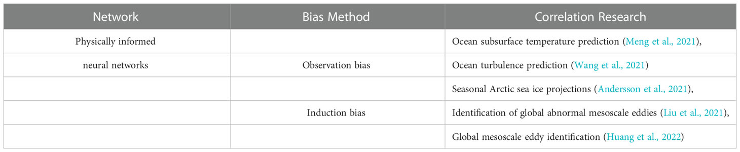
Table 3 Partial PINNs for marine science.

Although some researchers have attempted to predict the real ocean current field based on the isotropic properties of Navier–Stokes equations, physical information is still limited to observational traction using model data or inductive traction using existing network structures. On the contrary, neural networks are significantly integrated with domain knowledge in basic science, which adopted learning bias to improve the applicability of the model to physical data (Cranmer et al., 2020; Xiong et al., 2021).

The observation, induction, and learning bias can be embedded as physically informed methods for different stages of neural networks, which can organically integrate domain knowledge and neural networks. Compared with the traditional numerical differential equations, the PINNs have excellent robustness in handling noise entrainment within the data. In addition to this, theoretical foundations, such as quasigeostrophic, Rossby wave, Ekman drift, and eddy theory, transform into the learning bias that is an important guarantee for advancing scientific knowledge discovery. In summary, the potential of neural networks in marine science has not yet been fully exploited. In the future, the structure of the neural network should be based on the basic theory of marine science and further advance toward the “AI for ocean science.”

3.3. Mathematically driven neural network

As a data-driven method, neural networks can be regarded as a “black box,” lacking mathematical interpretability, which is the foundation of building bridges from data to knowledge. It is difficult to fully transform the neural network from a black box to a “white one.” However, neural networks can be improved based on the mathematical inference that makes partial network interpretability that is named mathematically driven neural networks. For example, the input and output of a neuron is a linear process that formulates as Equation (3).

$\begin{array}{ll}L={\displaystyle \sum _{i_0=0}^{d+1}}({\mathit{\text{a}}}_{i_1{i}_0}^0{\mathit{\text{x}}}_{i_0})& (3)\end{array}$

where a, x, d denote weight, input, and network width, respectively. Theoretically, the depth and width of a neural network can reach infinite dimensions and can be mathematically represented as an infinitely wide function space, constituting a mathematical “Barak space” (Wojtowytsch, 2020) as in Equation (4).

$\begin{array}{ll}{F}_{\infty }:=\left\{{\displaystyle \sum _{i_L=1}^{\infty }}{a}_{i_L}^L\sigma \left({\displaystyle \sum _{i_{L-1}}^{\infty }}{a}_{i_L{i}_{L-1}}^L\sigma \left({\displaystyle \sum _{i_{L-2}}}L\sigma \left(\left({\displaystyle \sum _{i_1=1}^{\infty }}{a}_{i_2{i}_1}^1\sigma \left({\displaystyle \sum _{i_0=0}^{d+1}}\left(a_{i_1{i}_0}^0{x}_{i_0}\right)\right)\right)\right)\right)\right)\right\}& (4)\end{array}$

where $a_{ij}^l=0$ for all but finitely many i, j, l. L is the layer number of a neural network, i_L is the neuron of every layer, and σ denotes the activation function. Furthermore, according to the geometrical point, high-dimensional data of the same category in nature is concentrated near some low-dimensional manifold. Therefore, the input of neural networks to the output can be understood as a mapping of differential geometric manifolds (Lei, 2020).

Based on the PINNs, the mathematically driven neural networks provide neural networks with a mathematical explanation. However, its theory, architecture, and application research are in the preliminary exploration stage. The mathematical theory not only bestowed the interpretability of networks, but also optimized computational efficiency and memory usage. Meanwhile, the properties of neural networks are exploited and compensate for the poor generalization ability of theoretical models to real data. In marine science, hydromechanics is the basic theory of how to introduce it into neural networks, constructing a novel marine physics or mathematical neural network structure as a frontier direction of future development. Moreover, it is able to exploit the excellent performance of deep neural networks in highly complex systems, accelerating knowledge discovery in marine science in massive data.

4. From DBAI to knowledge discovery

The surface data of the ocean obtained by satellite remote sensing is abundant, whereas the profile data of the intermediate ocean is relatively sparse. At present, the critical task of DBAI is to establish the intrinsic connection between surface phenomena and intermediate processes, especially the physical and ecological processes below the surface. With impressive results, the data-driven DBAI methodology has recently made a preliminary exploration of “surface to interior” in ocean science. However, ocean knowledge discovery methods mainly focus on associative statistical neural networks and begin to explode to the PINNs, the research of mathematically driven neural networks is still in exploration. In this review paper, highly challenging typical applications are selected from four aspects of marine morphology, kinematics, dynamics, and ecology to demonstrate intermediate ocean research supported by DBAI as shown in Figure 8.

FIGURE 8

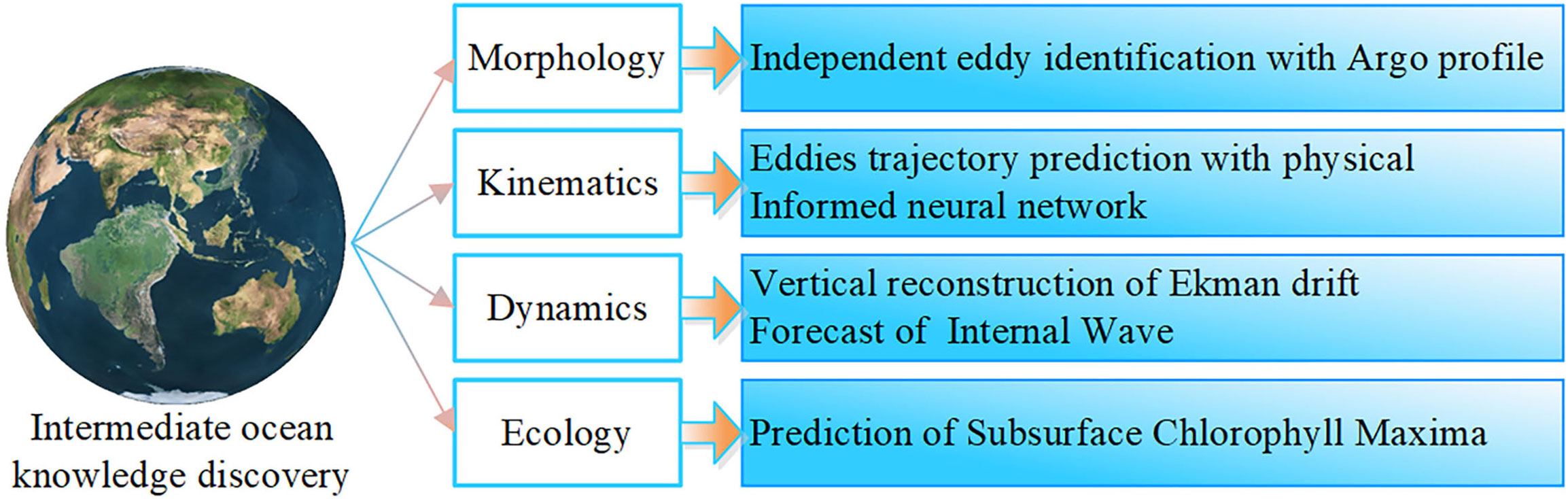
Figure 8 Typical applications in physical and biological oceanography with a top-down way of “surface to interior.”

4.1. 3-D identification and trajectory prediction of oceanic eddy

Oceanic mesoscale eddies, which follow the quasi-geostrophic potential vorticity conservation equation, are rotating movements of seawater on scales smaller than Rossby waves. Oceanic mesoscale eddies are the “weather” of the ocean with horizontal scales ranging from several to hundreds of kilometers, vertical scales ranging from tens to thousands of meters, and temporal scales from days to years. Ocean eddies, with their massive quantity, broad distribution, strong entrainment, and high energy, are becoming the ideal proxy for the substance cycling, energy cascade, and multi-sphere coupling in ocean research.

According to their rotation direction, oceanic eddies can be divided into cyclonic eddies (CE) and anticyclonic eddies (AE). The dynamic process of the water body inside the eddy is mapped to the sea surface, resulting in an undulating change in sea surface height of about 1~100 cm, which causes the topological relationship of the sea surface around the eddy to present a relatively stable closed structure. This phenomenon makes the formation of the local maximum (or minimum) value of sea surface height in the center of the AE (CE), which is the fundamental criteria of the application to detect ocean eddies with remote sensing technology (Pegliasco et al., 2022) as shown in Figure 9.

FIGURE 9

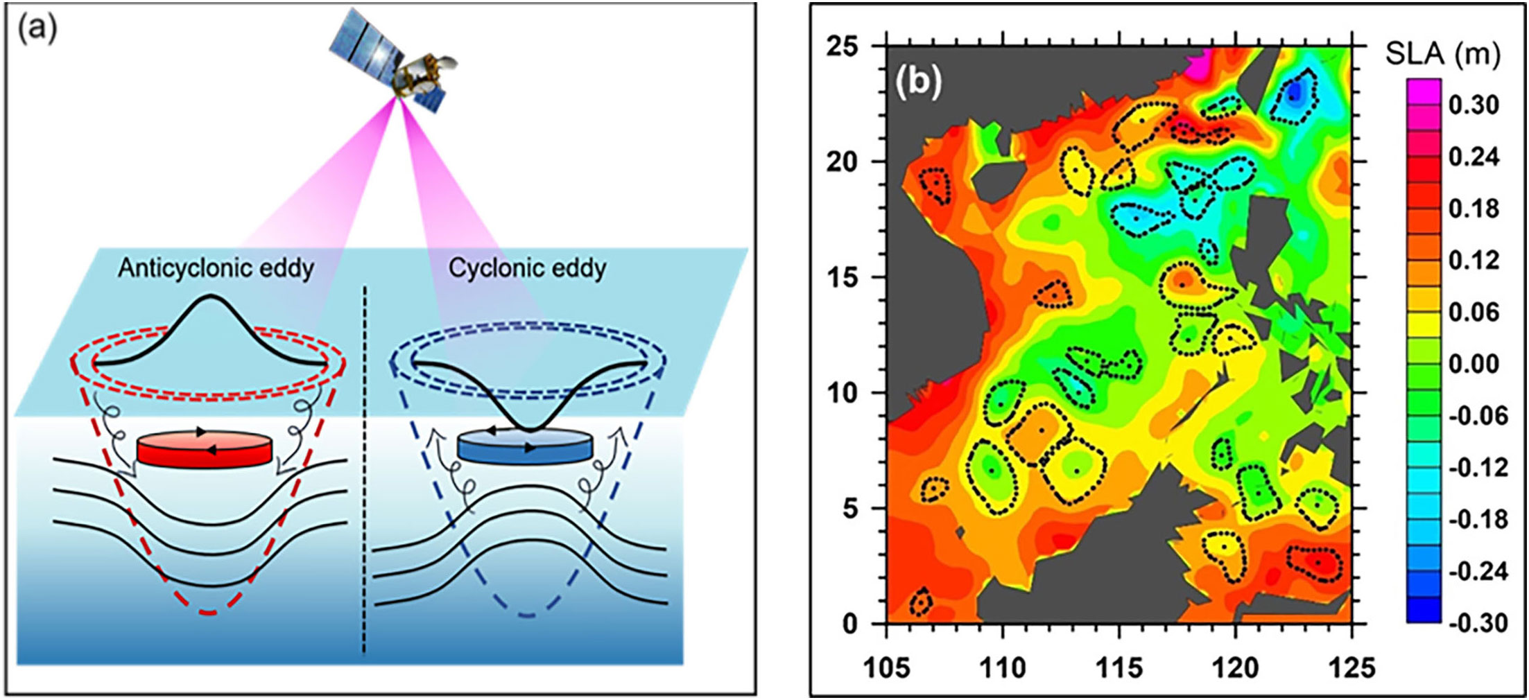
Figure 9 Oceanic detection and identification from the altimeter. (A) The fundamental criteria of the application to detect an ocean eddy, and (B) detection of eddies and identification results.

By combining the eddy signal acquired by satellite altimeter with in situ observations data such as Argo, the “surface-to-interior” vertical structure and internal dynamic process of the oceanic eddy are gradually being understood (Chaigneau et al., 2011; Zhang et al., 2014). However, the horizontal observation resolution and vertical profile detection capability of existing satellite altimeters are still inadequate. Hence, realizing high-resolution 3-D remote sensing observation of eddies is one of marine science’s urgent requirements for the new ocean satellite technology.

4.1.1. Independent eddy identification with Argo profiles

Eddy identification is critical in advancing theoretical knowledge and scientific research on ocean eddies. The current mainstream method of eddy identification is the closed contours method, which is limited by the sampling capacity of the satellite altimeter, resulting in approximately 90% of oceanic eddies being missed (Amores et al., 2018). In addition, this method has limitations for submesoscale eddies with the characteristics of having smaller scale, weaker intensity, and deeper below the sea surface.

To solve the above problem, an idea of ocean eddy identification based on 3-D structure is proposed by using profiling Argo (Chen et al., 2021a). The surface features of oceanic eddies are correlated and modeled with their vertical structures to construct an Argo floats-based algorithm for independent eddy identification. The altimeter-identified eddies are further aligned with Argo profiles to build a multisource eddy data set. The associative statistical neural network incorporating the observation and induction bias is designed to extract abstract features of the eddy vertical structure, thus realizing high-precision eddy identification from a 3-D perspective (Chen et al., 2021c; Huang et al., 2022) as illustrated in Figure 10A Compared with the traditional mathematical statistics methods, the AI eddy identification algorithm based on Argo 3-D structure not only improves the computational efficiency by more than 10 times, but also achieves 98% accuracy of eddy identification.

FIGURE 10

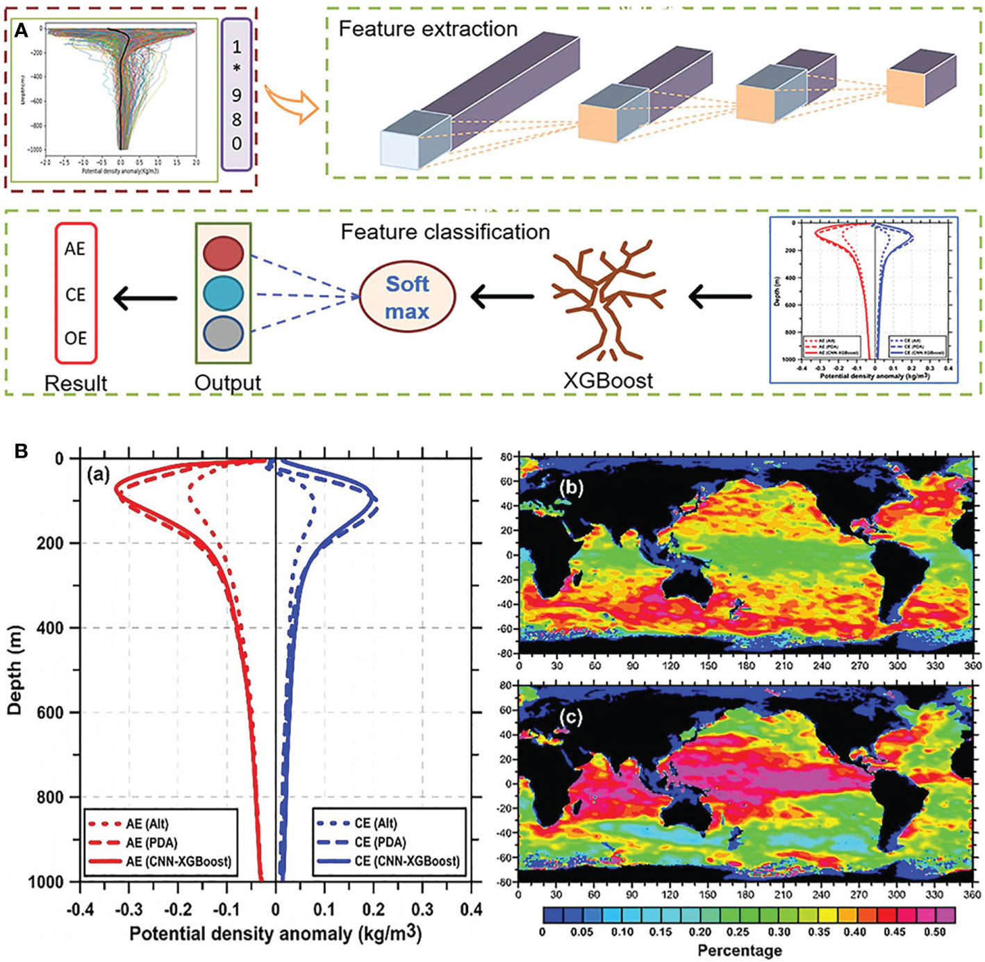
Figure 10 (A) The associative statistical neural network for eddy identification with Argo profiles calibrated by the altimeter. (B) Comparison of eddy identification results between altimeter and Argo. Independent eddy identification with Argo profiles via associative statistical neural network. (10a) The architecture of convolutional neural network with extreme gradient boosting (CNN-XGBoost). (10b) Identification results. (a) Vertical profiles of eddies identified by altimeter (short dashed line) and only Argo (solid and long dashed lines), respectively, (b) Global geographical distribution of identified eddies by altimeter, and (c) global geographical distribution of independently identified eddies by Argo profiles.

The eddy vertical identification algorithm can identify about 36% of the missed eddies. This method can prompt additional consideration of the eddy identification accuracy from satellite altimeter. Figure 10B shows the comparison results of eddy identification using altimeter SLA and the Argo vertical profiles, respectively. The experimental results show that more than 50% of the eddies missed by the altimeter are distributed in the equatorial region with a low satellite sampling rate, weak geostrophic, and strong non-geostrophic. In contrast, the Argo vertical eddy identification algorithm has a unique advantage in non-geostrophic dominated submesoscale eddy identification, which is highly complementary to the altimeter eddy identification method. In addition, the Argo vertical signal of eddies captured by the AI eddy identification algorithm is comparable to or even stronger than the altimeter method. The AI technology demonstrates the feasibility and credibility of eddy identification with 3-D ocean profiles while innovating identification methods and improving identification efficiency. This is essential for promoting the development of eddy identification methods and studying ocean eddies’ kinematics and dynamics.

4.1.2. Eddies trajectory prediction with PINN

Eddy motion is primarily prevalent in complex ocean environments (current, wind, and topographic) and is controlled by various physical mechanisms, including potential vorticity and baroclinic instability (Chen et al., 2022a). Naturally, the accuracy of eddy trajectory prediction can be fundamentally improved with the physical constraint of prior knowledge. The eddy trajectory prediction network compliant with physical constraint is proposed as shown in Figure 11A The theoretical approximate phase speed of the first baroclinic mode Rossby waves (C_p) is embedded as the theoretical velocity of the vortex into the machine learning model for trajectory prediction, thus enabling accurate prediction of the eddy trajectory for the next 10 days.

FIGURE 11

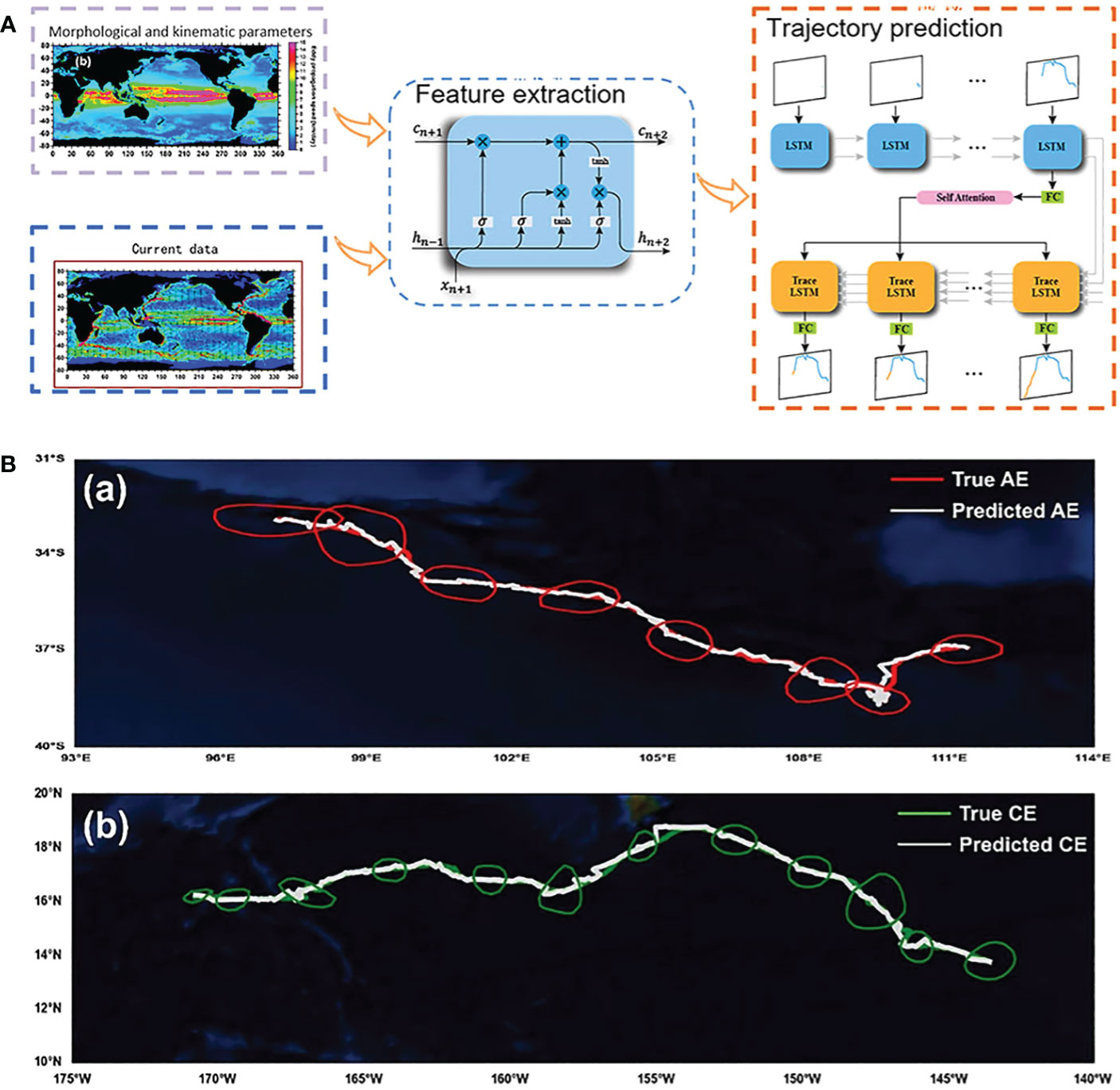
Figure 11 (A) The physically informed neural network for eddy trajectory prediction. (B) Long-lived eddies trajectory prediction.Eddy trajectory prediction via associative neural network. (A) The architecture of the eddy trajectory prediction network compliant with physical constraints. (B) Results of long-lived eddies trajectory prediction. (a) AE trajectory prediction, (b) CE trajectory prediction.

$\begin{array}{ll}{C}_p=-\beta \times R_d^2& (5)\end{array}$

where β = 2Ωcos θR^-1 is the Rossby parameter, ω = 7.29×10⁵ is an Earth rotation rate, and R = 6371.39 km is the radius of Earth. R_d is the Rossby radius of deformation, which is calculated (Chelton et al., 1998) by Equation (6):

$\begin{array}{ll}{R}_d=\frac{1}{\left|f\left(\theta \right)\right|\pi }{\displaystyle {\int }_{-H}^0}N\left(z\right)dz(\theta >5^{\circ })& (6)\end{array}$

where f = 2Ωθ is the Coriolis parameter, N(z)=(−(g/ρ)×∂ρ(z)/∂z)^1/2 is the buoyancy frequency, ρ is the potential density, and g is the acceleration due to gravity. The midterm prediction results for more than two million single-track eddies worldwide show that the accuracy of eddy trajectory prediction is improved by about 24% with the embedding of the physical mechanism, and the prediction error is significantly lower than other prediction algorithms (Li et al., 2019; Wang et al., 2022). Figure 11B illustrates the true and predicted trajectories of two typical long-lived eddies. The results visually demonstrate the high consistency between the predicted trajectories and the true trajectories, reflecting the significant advantages of the PINN for eddy trajectory prediction.

4.2. Vertical reconstruction of Ekman drift

The wind is the dominant driving mechanism of ocean circulation. When the wind with constant speed abidingly acts on the vast sea expanse, a steady seawater movement is generated, called drift. Ekman has constructed a precise theoretical drift solution, namely, the Ekman drift theory. Specifically, the drift is the result of the balance between the frictional force generated by the plumb turbulence and the Coriolis force. The latitudinal velocity component (u) and the meridional velocity component (v) of the drift are affected by the depth of seawater (z), and their quantified expressions are shown in Equations (7) and (8).

$\begin{array}{ll}u=\frac{{\tau }_y}{\sqrt{2}a{A}_z}\exp (az)\cos {45}^{\circ }+az,& (7)\end{array}$

$\begin{array}{ll}v=\frac{{\tau }_y}{\sqrt{2}a{A}_z}\exp (az)\sin {45}^{\circ }+az& (8)\end{array}$

Ekman found that the surface current direction is approximately 45° to the right (left) of the wind direction in the Northern (Southern) hemisphere with ideal assumptions. Due to the viscosity of seawater, the flow vector deflects with depth and forms an Ekman spiral as shown in Figure 12A. The simple assessment of global wind-driven drift can be calculated using satellite scatterometer data on sea surface wind fields as illustrated in Figure 12B. However, in the natural ocean, the turbulent viscosity coefficient A_z varies with depth, and the latitudinal wind stress τ_x effect exists simultaneously, coupled with the fact that the wind-driven drift decays faster with depth than the theoretical prediction. These reasons cause the actual profile of wind-generated drift to be different from the theoretical Ekman spiral curve, and its shape is closely related to the sea state of the local ocean. In addition, due to the lack of observational information on the seawater turbulent viscosity coefficient, the two-parameter regression model is used as the mainstream method to reconstruct the wind current field (Lagerloef et al., 1999). The core algorithm of this model is to evaluate wind current using the observations of the in situ drifting buoy in the field without the ground-transfer current component. However, the limitation is that the model accuracy is affected by empiricism or climatological parameters. AI technology, as a data-driven method, can effectively avoid the empiricism of the model and have some stability to the climatological parameters in the reconstruction process. Therefore, with the introduction of the DBAI methodology, the accurate quantification of wind-driven current fields is expected to expand novel ideas and methods.

FIGURE 12

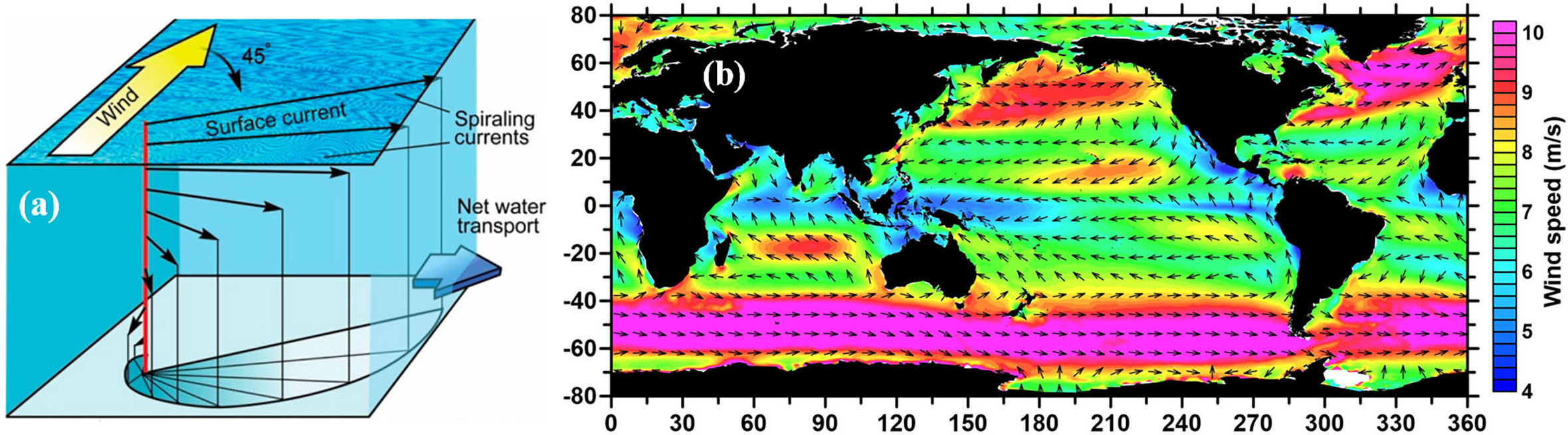
Figure 12 Ekman spiral. (A) Simulation model of Ekman spiral, (B) Global sea surface wind speed distribution.

4.3. Forecast of IWs

IWs are fluctuations that oscillate at the surface of two different media within the ocean. Two necessary conditions for generating IWs are seawater stratification and a disturbance source. The wavelength of IWs generally ranges from hundreds of meters to tens of kilometers, period ranges from minutes to hours, and amplitude ranges from several meters to tens of meters. IWs mainly occur in the pycnocline and are most active at 50–800 m of the ocean. In addition, the undulating propagation of IWs and its “dead water effect” affect local ocean productivity and ocean sound field and even cause great security risks to submarine navigation and ocean engineering.

The synthetic aperture radar (SAR) has become one of the essential remote-sensing tools for monitoring ocean IWs with its observation advantages of large range, all day, all weather, and high resolution. The quantitative expression of the modulation of SAR images by IWs can be derived based on the Korteweg–de Vries (KdV) Equation (9) (Zheng et al., 2001).

$\begin{array}{ll}{\delta }_{0|IW}=Q\left(\frac{C{\eta }_{0}co{s}^2\phi }{h_{md}\Delta \varpi }\right)tg{h}_{wd}\left[\frac{\left(x-Vt\right)}{\Delta }\right]sec\left(h_{wd}^2\right)\left[\frac{\left(x-Vt\right)}{\Delta }\right]& (9)\end{array}$

where δ_0|IW is the backscattering coefficient of the IWs on the SAR image; Q can be treated approximately as a constant, usually determined by the SAR sensor frequency, the angle of incidence, and the dielectric constant of the IWs. C is the linear phase speed; φ is the wave direction; h_md is the thickness of the mixing layer; Δ is the characteristic half width of the IWs; ϖ is the mean value of angular frequency of ocean surface waves; g, h_wd, x, V, t represent the acceleration due to gravity, seawater depth, spatial position, propagation speed, and propagation time of the IWs, respectively. sec(g)is secant function. Equation (9) is also known as the analytical expression of the oceanic IWs presented on the SAR image. Therefore, the spatial position, wavelength, wave direction, and other horizontal parameter information of the IWs can be directly obtained from SAR images. The transient wave speed, depth, amplitude, and other vertical parameters of IWs can then be further inverted, together with the simultaneously measured CTD and historical data to depict the spatial and temporal characteristics of IWs properly as shown in Figure 13.

FIGURE 13

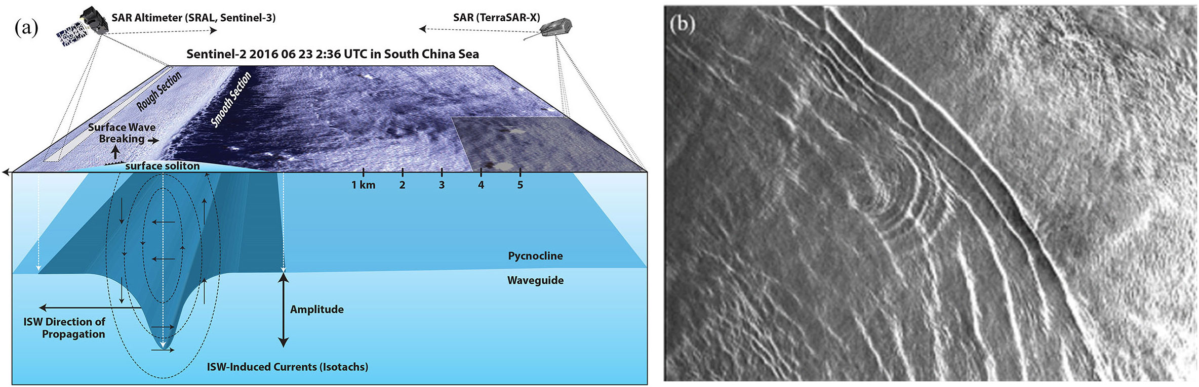
Figure 13 Oceanic IWs. (A) IWs mechanism for modulated SAR images, (B) IWs on SAR images (Magalhães et al., 2021).

In recent years, DBAI has been applied successfully to the inversion and prediction of oceanic IWs from satellite images. An associative statistical neural network structure is proposed to address the randomness issue with IWs propagation (Zhang et al., 2021). This network mines the correlation between multiple information of IWs and determines the propagation position of IWs by predicting the propagation speed and direction. Comparisons with the conventional physical model (KdV equation) results show that the neural network can achieve better performance and robustness as shown in Figure 14. This research also further reveals the effect of complicated seafloor topography on IW propagation. Another scholar used the IW amplitudes simulated by physical oceanographic equipment as auxiliary data. The information between the auxiliary data and the spectral characteristics of remote sensing satellite images (MODIS) is correlated and migrated by observational neural networks to invert the IWs amplitudes (Zhang et al., 2022).

FIGURE 14

Figure 14 (A) The associative statistical neural network for IWs forecasting. (B) Forecast results of the IWs. Interval wave forecasting from satellite images. (A) The architecture of IWs forecasting neural network. (B) Forecast of IW propagations in the Andaman Sea after two semidiurnal tidal cycles. (A) shows the results of the associative statistical neural network, and (B) shows the results of the KdV equation (Zhang et al., 2021).

The application of DBAI technology in oceanic IWs is still in the exploration stage. These methods mainly learn the deep features of IWs through a large amount of remote sensing data rather than constructing an exclusive structure of PINNs on the mechanism of IWs generation. Nevertheless, the feasibility of applying DBAI technology to oceanic IWs is confirmed, providing a novel idea for studying oceanic IWs.

4.4. Prediction of subsurface chlorophyll maxima

Biomass distribution is as important in the subsurface ocean as stratification structural features, whereas most of the water color remote sensing satellites can only directly acquire the chlorophyll concentration [Chla]_sur from the sea surface. To invert chlorophyll vertical distribution from the sea surface chlorophyll concentration [Chla]_sur based on a large number of in situ observations, the models of chlorophyll concentration content and its vertical distribution were constructed for different stratified water bodies and trophic levels, integrated over the euphotic layer (Uitz et al., 2006). The detailed calculations of the different models are shown in Equations (10) and (11).

$\begin{array}{ll}Chl{a}_{Z_{eu}}=A·{[Chla]}_{sur}^B& (10)\end{array}$

$\begin{array}{ll}C\left(\zeta \right)=c_0-c_1·\zeta +c_2·exp-{[\left(\zeta -c_3\right)/c_4]}^2& (11)\end{array}$

where Chla_Zeu represents the chlorophyll a content integrated over the euphotic zone, ς is the normalized value of the actual depth relative to the depth of the euphotic layer Z_eu, i.e., ς = z/Z_eu, C(ς) denotes the normalized value of chlorophyll a concentration [Chla(ς)] at depth ς relative to the average chlorophyll concentration $\overline{{[Chla]}_{Zeu}}$ within the euphotic layer, i.e., $C\left(\varsigma \right)=\left[Chla\left(\varsigma \right)\right]/\overline{{[Chla]}_{Zeu}}$, among them, $\overline{{[Chla]}_{Zeu}}=Z_{eu}^{-1}·Chl{a}_{Zeu}$. Furthermore, the parameters A, B and c₀~c₄ in (10) and (11) can be obtained by fitting the field data of different stratified water bodies and trophic levels (Uitz et al., 2006). It can be seen that chlorophyll a vertical distribution of well-mixed waters ($\frac{Z_m}{Z_{eu}}>1$, Z_m is the depth of mixed layer) is relatively uniform. In contrast, for stratified water bodies ($\frac{Z_m}{Z_{eu}}<1$), SCM is generally present in the vertical profile. On the one hand, SCM plays a crucial role in ocean nutrient cycling, energy flow, and biogeochemical cycling, and on the other hand, the chlorophyll vertical distribution, especially the inversion of SCM, is important for accurate estimation of ocean primary productivity. However, the SCM features have been explored only at the regional scale due to the lack of 3-D observation data. With the implementation of the BGC-Argo program, it has become possible to analyze SCM on a global scale while revealing that the seasonal dynamics of SCM have an evident regional character (Cornec et al., 2021).

With the accumulation of biogeochemical 3-D observation data and the development of computer technology, there is an increasing amount of research related to applying neural networks to chlorophyll vertical structure inversion. The associative statistical neural network was developed as shown in Figure 15A and successfully inverted the vertical structure of SCM in the North Pacific region using sea surface parameters observed by satellite remote sensing (Chen et al., 2022b). The application of AI technology to the inversion and prediction of marine SCM can take full advantage of long-term and high-coverage satellite data to obtain the global oceanic SCM data set indirectly, the results are illustrated in Figure 15B. It is crucial for advancing marine ecology and related multidisciplinary research because it provides data for exploring the vertical ecological structure of the ocean.

FIGURE 15

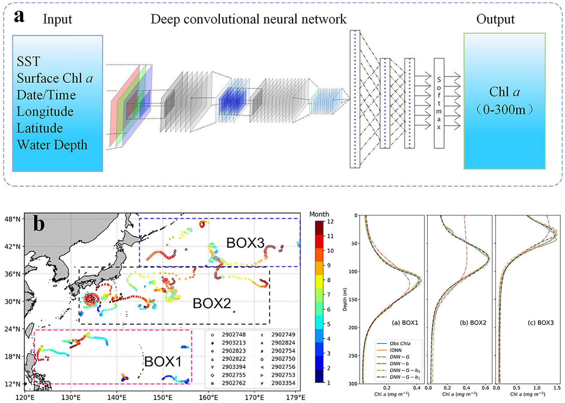
Figure 15 (A) The SCM perception network. (B) SCM predictions results. Prediction of SCM. (A) The architecture of SCM prediction neural network. (B) Comparisons of the mean profiles of observed values(blue line), associative statistical neural network predictions (orange line), and multi layer perceptron predictions (green dash line) inferred from remote sensing data in three boxes.

5. Conclusions and discussion

From the theoretical development of marine science, the progress of basic theory, observation technology, and computing ability have been drawing and responding to each other, pushing forward the leaps of this interdisciplinary science one after another. Before the middle of the last century, the development of marine science mainly benefited from advances in theory. Based on the limited field observation data, Ekman drift theory, Rossby planetary wave theory, westward strengthening theory of ocean circulation, wind-induced ocean circulation theory, and so on were developed successively, laying the theoretical foundation of modern physical oceanography.

From the perspective of marine science development in the 1970s, the emergence of satellite ocean remote sensing for scientific research provides unprecedented high spatial and temporal coverage data. With remote sensing data, it is the first time to realize the clear appearance of ocean circulation, qualify the global average sea level rise, estimate the global marine primary productivity, etc. Subsequently, the rapid development of computer technology has brought about a significant improvement in computing power, and model systems with high resolution have begun to shine in the cutting-edge applications of operational weather forecasting and climate change prediction. At the end of the 20th century, to jointly cope with the severe challenges brought by global changes, oceanographers devoted themselves to studying the processes occurring in the intermediate and deep sea, filling in the gaps of the existing theoretical system and no longer satisfied with the understanding of the ocean surface and phenomena at large space–time scale.

In this context, the in situ observation technology provides profile data to implement research from surface ocean phenomena to intermediate ocean dynamic and ecological processes. Naturally, how to reveal the intermediate ocean law from the mass fusion data has become a major challenge. “AI for science” has spawned a new paradigm of scientific research, and AI has also become a strategic technology for new scientific research. The development of AI technology requires not only a breakthrough in computational theory but also a full integration of interdisciplinary knowledge. The ultimate goal of AI is to train machines to be brain-like, bridging the knowledge between the human brain and the machine. Moreover, the natural combination of AI technology and oceanography (DBAI method) provides an excellent way to solve the current development dilemma of oceanography. The two have built a new bridge between data science and knowledge discovery, and initially showed unique advantages and great potential in intermediate ocean remote sensing applications from the outside to the inside.

DBAI is poised to achieve “surface-to-interior” knowledge of the middle ocean remote sensing and its processes, covering for the inadequacy of the existing theoretical system. However, the intermediate ocean remote sensing technology supported by AI is still facing two major challenges, one is the ocean data bottleneck the other is the generalization of DBAI methodology. Therefore, we believe that future trends in DBAI will focus on the following two points.

(1) Promote the construction of ocean big data. To fill the current gaps in some ocean parameters and underwater 3-D remote sensing, the development of a new generation of ocean science satellites (e.g., SWOT, Guanlan) is expected to enhance the comprehensive capabilities of satellites in horizontal space, vertical profile, spatial and temporal resolution, and integrated remote sensing. The cornerstone of DBAI is marine big data. With access to massive remote sensing data, the biggest obstacle to the development of DBAI is how to provide reliable ground truth to express information about marine objects. If we want to break through this obstacle, relying on one person or team is unrealistic. Therefore, we should actively participate in ocean big data construction plans, implement extensive international cooperation, and promote the construction of standard marine big data sets.

(2) Strengthening DBAI technology innovation. Most DBAI technologies for ocean science come from the computer-vision community. These techniques aim to enable computers to obtain meaningful pattern information from images, videos, and other visual inputs, often focusing on spatial patterns. These models can be used to construct oceanographic AI models with physical interpretability by combining oceanographic mechanism constraints with remote sensing data-driven to achieve theoretical and technological innovations in DBAI.

With the gradual enrichment of ocean big data sets and the continuous improvement of DBAI technology, DBAI will be widely applied in various marine subdivisions to realize automatic or semiautomatic scientific discovery. We envisage that the new scientific research paradigm of “AI for ocean science” will gradually uncover the mystery of intermediate and even deep oceans, ushering in a new phase in the future of ocean science.

Author contributions

GC conceived the study, co-designed and contributed to data collection, undertook analysis, and led the drafting of the manuscript. BH, JY, and MR co-designed and contributed to data collection, undertook analysis, and contributed to the drafting of the manuscript. LG, CC, XC, LX, GH, and YM contributed to data collection, data analysis, and wrote sections of the manuscript. All authors contributed to manuscript revision, read, and approved the submitted version.

Funding

This research was jointly supported by the National Natural Science Foundation of China (NO. 42030406 and No. 42276203) and the Natural Science Foundation of Shandong Province (No. ZR2021MD001).

Conflict of interest

The authors declare that the research was conducted in the absence of any commercial or financial relationships that could be construed as a potential conflict of interest.

Publisher’s note

All claims expressed in this article are solely those of the authors and do not necessarily represent those of their affiliated organizations, or those of the publisher, the editors and the reviewers. Any product that may be evaluated in this article, or claim that may be made by its manufacturer, is not guaranteed or endorsed by the publisher.

References

Accarino G., Chiarelli M., Fiore S., Federico I., Causio S., Coppini G., et al. (2021). A multi-model architecture based on long short-term memory neural networks for multi-step sea level forecasting. Future Generation Comput. Syst. 124, 1–9. doi: 10.1016/j.future.2021.05.008

CrossRef Full Text | Google Scholar

Amani M., Ghorbanian A., Asgarimehr M., Yekkehkhany B., Moghimi A., Jin S., et al. (2021). Remote sensing systems for ocean: A review (part 1: Passive systems). IEEE J. Selected Topics Appl. Earth Observations Remote Sens. 15, 210–234. doi: 10.1109/JSTARS.2021.3130789

CrossRef Full Text | Google Scholar

Amani M., Mehravar S., Asiyabi R. M., Moghimi A., Ghorbanian A., Ahmadi S. A., et al. (2022a). Ocean remote sensing techniques and applications: A review (part ii). Water 14, 3401. doi: 10.3390/w14213401

CrossRef Full Text | Google Scholar

Amani M., Moghimi A., Mirmazloumi S. M., Ranjgar B., Ghorbanian A., Ojaghi S., et al. (2022b). Ocean remote sensing techniques and applications: A review (part i). Water 14, 3400. doi: 10.3390/w14213400

CrossRef Full Text | Google Scholar

Amani M., Mohseni F., Layegh N. F., Nazari M. E., Fatolazadeh F., Salehitangrizi A., et al. (2022c). Remote sensing systems for ocean: A review (part 2: Active systems). IEEE J. Selected Topics Appl. Earth Observations Remote Sens 15, 1421–1453. doi: 10.1109/JSTARS.2022.3141980

CrossRef Full Text | Google Scholar

Amores A., Jordà G., Arsouze T., Le Sommer J. (2018). Up to what extent can we characterize ocean eddies using present-day gridded altimetric products? J. Geophysical Research: Oceans 123, 7220–7236. doi: 10.1029/2018JC014140

CrossRef Full Text | Google Scholar

Andersson T. R., Hosking J. S., Pérez-Ortiz M., Paige B., Elliott A., Russell C., et al. (2021). Seasonal arctic sea ice forecasting with probabilistic deep learning. Nat. Commun. 12, 5124. doi: 10.1038/s41467-021-25257-4

PubMed Abstract | CrossRef Full Text | Google Scholar

Appenzeller T. (2021). The AI revolution in science. report 16. (Washington, United States: American Association for the Advancement of Science).

Google Scholar

Behrenfeld M. J., Gaube P., Della Penna A., O’Malley R. T., Burt W. J., Hu Y., et al. (2019). Global satellite-observed daily vertical migrations of ocean animals. Nature 576, 257–261. doi: 10.1038/s41586-019-1796-9

PubMed Abstract | CrossRef Full Text | Google Scholar

Behrenfeld M. J., Hu Y., Hostetler C. A., Dall’Olmo G., Rodier S. D., Hair J. W., et al. (2013). Space-based lidar measurements of global ocean carbon stocks: Space lidar plankton measurements. Geophysical Res. Lett. 40, 4355–4360. doi: 10.1002/grl.50816

CrossRef Full Text | Google Scholar

Behrenfeld M. J., Hu Y., O’Malley R. T., Boss E. S., Hostetler C. A., Siegel D. A., et al. (2017). Annual boom–bust cycles of polar phytoplankton biomass revealed by space-based lidar. Nat. Geosci. 10, 118–122. doi: 10.1038/ngeo2861

CrossRef Full Text | Google Scholar

Chaigneau A., Le Texier M., Eldin G., Grados C., Pizarro O. (2011). Vertical structure of mesoscale eddies in the eastern south pacific ocean: A composite analysis from altimetry and argo profiling floats. J. Geophysical Research: Oceans 116, 1–16. doi: 10.1029/2011JC007134

CrossRef Full Text | Google Scholar

Chelton D. B., deSzoeke R. A., Schlax M. G., El Naggar K., Siwertz N. (1998). Geographical variability of the first baroclinic rossby radius of deformation. J. Phys. Oceanography 28, 433–460. doi: 10.1175/1520-0485(1998)028<0433:GVOTFB>2.0.CO;2

CrossRef Full Text | Google Scholar

Chen G., Chen X., Cao C. (2022a). Divergence and dispersion of global eddy propagation from satellite altimetry. J. Phys. Oceanography 52, 705–722. doi: 10.1175/JPO-D-21-0122.1

CrossRef Full Text | Google Scholar

Chen X., Chen G., Ge L., Huang B., Cao C. (2021c). Global oceanic eddy identification: A deep learning method from argo profiles and altimetry data. Front. Mar. Sci. 8, 21–35. doi: 10.3389/fmars.2021.646926

CrossRef Full Text | Google Scholar

Chen G., Chen X., Huang B. (2021a). Independent eddy identification with profiling argo as calibrated by altimetry. J. Geophysical Research: Oceans 126, 1–22. doi: 10.1029/2020JC016729

CrossRef Full Text | Google Scholar

Chen J., Gong X., Guo X., Xing X., Lu K., Gao H., et al. (2022b). Improved perceptron of subsurface chlorophyll maxima by a deep neural network: A case study with bgc-argo float data in the northwestern pacific ocean. Remote Sens. 14, 632. doi: 10.3390/rs14030632

CrossRef Full Text | Google Scholar

Chen P., Jamet C., Zhang Z., He Y., Mao Z., Pan D., et al. (2021b). Vertical distribution of subsurface phytoplankton layer in south china sea using airborne lidar. Remote Sens. Environ. 263, 112567. doi: 10.1016/j.rse.2021.112567

CrossRef Full Text | Google Scholar

Chen L.-C., Papandreou G., Kokkinos I., Murphy K., Yuille A. L. (2018). Deeplab: Semantic image segmentation with deep convolutional nets, atrous convolution, and fully connected crfs. IEEE Trans. Pattern Anal. Mach. Intell. 40, 834–848. doi: 10.1109/TPAMI.2017.2699184

PubMed Abstract | CrossRef Full Text | Google Scholar

Chen G., Tang J., Zhao C., Wu S., Yu F., Ma C., et al. (2019). Concept design of the “guanlan” science mission: China’s novel contribution to space oceanography. Front. Mar. Sci. 6, 194–208. doi: 10.3389/fmars.2019.00194

CrossRef Full Text | Google Scholar

Chepfer H., Noel V., Chiriaco M., Wielicki B., Winker D., Loeb N., et al. (2018). The potential of a multidecade spaceborne lidar record to constrain cloud feedback. J. Geophysical Research: Atmospheres 123, 5433–5454. doi: 10.1002/2017JD027742

CrossRef Full Text | Google Scholar

Churnside J. H. (2013). Review of profiling oceanographic lidar. Optical Eng. 53, 51405. doi: 10.1117/1.OE.53.5.051405

CrossRef Full Text | Google Scholar

Cornec M., Laxenaire R., Speich S., Claustre H. (2021). Impact of mesoscale eddies on deep chlorophyll maxima. Geophysical Res. Lett. 48, 1–10. doi: 10.1029/2021GL093470

CrossRef Full Text | Google Scholar

Cozman F. (2021). How ai is helping the natural sciences. Artif. Intell. 598, S5–S7. doi: 10.1038/d41586-021-02762-6

CrossRef Full Text | Google Scholar

Cranmer M., Greydanus S., Hoyer S., Battaglia P., Spergel D., Ho S. (2020). “Lagrangian Neural networks,” in ICLR 2020 Workshop on Integration of Deep Neural Models and Differential Equations. 1–9 (Addis Ababa, Ethiopia: https://OpenReview.net).

Google Scholar

George T. M., Manucharyan G. E., Thompson A. F. (2021). Deep learning to infer eddy heat fluxes from sea surface height patterns of mesoscale turbulence. Nat. Commun. 12, 800. doi: 10.1038/s41467-020-20779-9

PubMed Abstract | CrossRef Full Text | Google Scholar

Goodfellow I. J., Pouget-Abadie J., Mirza M., Xu B., Warde-Farley D., Ozair S., et al. (2014). “Generative adversarial nets,” in The international conference on neural information processing systems (Cambridge, MA, USA: MIT Press), 2672–2680. NIPS’14.

Google Scholar

Greydanus S., Dzamba M., Yosinski J. (2019). “Hamiltonian Neural networks,” in The international conference on neural information processing systems(Vancouver, Canada: Curran Associates, Inc) 1–11.

Google Scholar

Ham Y.-G., Kim J.-H., Luo J.-J. (2019). Deep learning for multi-year enso forecasts. Nature 573, 568–572. doi: 10.1038/s41586-019-1559-7

PubMed Abstract | CrossRef Full Text | Google Scholar

He K., Gkioxari G., Dollar P., Girshick R. (2017). “Mask r-cnn,” in IEEE International conference on computer vision (Venice: IEEE), 2980–2988. doi: 10.1109/ICCV.2017.322

CrossRef Full Text | Google Scholar

He K., Zhang X., Ren S., Sun J. (2016). “Deep residual learning for image recognition,” in 2016 IEEE conference on computer vision and pattern recognition (Las Vegas, NV, USA: IEEE), 770–778. doi: 10.1109/CVPR.2016.90

CrossRef Full Text | Google Scholar

Hostetler C. A., Behrenfeld M. J., Hu Y., Hair J. W., Schulien J. A. (2018). Spaceborne lidar in the study of marine systems. Annu. Rev. Mar. Sci. 10, 121–147. doi: 10.1146/annurev-marine-121916-063335

CrossRef Full Text | Google Scholar

Huang B., Ge L., Chen X., Chen G. (2022). Vertical structure-based classification of oceanic eddy using 3-d convolutional neural network. IEEE Trans. Geosci. Remote Sens. 60, 1–14. doi: 10.1109/TGRS.2021.3103251

CrossRef Full Text | Google Scholar

Huang G., Liu Z., van der Maaten L., Weinberger K. Q. (2017). “Densely connected convolutional networks,” in 2017 IEEE conference on computer vision and pattern recognition (CVPR) (Honolulu, HI: IEEE), 2261–2269. doi: 10.1109/CVPR.2017.243

CrossRef Full Text | Google Scholar

Jian M., Liu X., Luo H., Lu X., Yu H., Dong J. (2021). Underwater image processing and analysis: A review. Signal Processing: Image Communication 91, 116088. doi: 10.1016/j.image.2020.116088

CrossRef Full Text | Google Scholar

Jian M., Qi Q., Dong J., Yin Y., Lam K.-M. (2018). Integrating qdwd with pattern distinctness and local contrast for underwater saliency detection. J. Visual communication image representation 53, 31–41. doi: 10.1016/j.jvcir.2018.03.008

CrossRef Full Text | Google Scholar

Jian M., Qi Q., Yu H., Dong J., Cui C., Nie X., et al. (2019). The extended marine underwater environment database and baseline evaluations. Appl. Soft Computing 80, 425–437. doi: 10.1016/j.asoc.2019.04.025

CrossRef Full Text | Google Scholar

Johnson G. C., Hosoda S., Jayne S. R., Oke P. R., Riser S. C., Roemmich D., et al. (2022). Argo–two decades: Global oceanography, revolutionized. Annu. Rev. Mar. Sci. 14, 379–403. doi: 10.1146/annurev-marine-022521-102008

CrossRef Full Text | Google Scholar

Karniadakis G. E., Kevrekidis I. G., Lu L., Perdikaris P., Wang S., Yang L. (2021). Physics-informed machine learning. Nat. Rev. Phys. 3, 422–440. doi: 10.1038/s42254-021-00314-5

CrossRef Full Text | Google Scholar

Lagerloef G. S. E., Mitchum G. T., Lukas R. B., Niiler P. P. (1999). Tropical pacific near-surface currents estimated from altimeter, wind, and drifter data. J. Geophysical Research: Oceans 104, 23313–23326. doi: 10.1029/1999JC900197

CrossRef Full Text | Google Scholar

Lecun Y., Bottou L., Bengio Y., Haffner P. (1998). Gradient-based learning applied to document recognition. Proc. IEEE 86, 2278–2324. doi: 10.1109/5.726791

CrossRef Full Text | Google Scholar

Lei N. (2020). A geometric understanding of deep learning. Engineering 6, 361–374. doi: 10.1016/j.eng.2019.09.010

CrossRef Full Text | Google Scholar

Li G., Cheng L., Zhu J., Trenberth K. E., Mann M. E., Abraham J. P. (2020). Increasing ocean stratification over the past half-century. Nat. Climate Change 10, 1116–1123. doi: 10.1038/s41558-020-00918-2

CrossRef Full Text | Google Scholar

Liu Y., Zheng Q., Li X. (2021). Characteristics of global ocean abnormal mesoscale eddies derived from the fusion of sea surface height and temperature data by deep learning. Geophysical Res. Lett. 48, 1–11. doi: 10.1029/2021GL094772

CrossRef Full Text | Google Scholar

Li J., Wang G., Xue H., Wang H. (2019). A simple predictive model for the eddy propagation trajectory in the northern south china sea. Ocean Sci. 15, 401–412. doi: 10.5194/os-15-401-2019

CrossRef Full Text | Google Scholar

Lu X., Hu Y., Yang Y., Bontempi P., Omar A., Baize R. (2020). Antarctic Spring ice-edge blooms observed from space by icesat-2. Remote Sens. Environ. 245, 111827. doi: 10.1016/j.rse.2020.111827

CrossRef Full Text | Google Scholar

Magalhães J. M., Alpers W., Santos-Ferreira A. M., Da Silva J. C. (2021). Surface wave breaking caused by internal solitary waves. Oceanography 34, 166–176. doi: 10.5670/oceanog.2021.203

CrossRef Full Text | Google Scholar

Meng Y., Rigall E., Chen X., Gao F., Dong J., Chen S. (2021). “Physics-guided generative adversarial networks for sea subsurface temperature prediction,” in IEEE Transactions on neural networks and learning systems. (Piscataway, United States: IEEE), 1–14. doi: 10.1109/TNNLS.2021.3123968

CrossRef Full Text | Google Scholar

Meng L., Yan X.-H. (2022). “Remote sensing for subsurface and deeper oceans: An overview and a future outlook,” in IEEE Geoscience and remote sensing magazine. Piscataway, United States, IEEE, 2–22. doi: 10.1109/MGRS.2022.3184951

CrossRef Full Text | Google Scholar

Morel A., Berthon J.-F. (1989). Surface pigments, algal biomass profiles, and potential production of the euphotic layer: Relationships reinvestigated in view of remote-sensing applications: Production computed from space-acquired data. Limnology Oceanography 34, 1545–1562. doi: 10.4319/lo.1989.34.8.1545

CrossRef Full Text | Google Scholar

Nakajima M., Tanaka K., Hashimoto T. (2021). “Neural schrödinger equation: Physical law as deep neural network,” in IEEE Transactions on neural networks and learning systems. (Piscataway, United States: IEEE), 1–15. doi: 10.1109/TNNLS.2021.3120472

CrossRef Full Text | Google Scholar

Pegliasco C., Delepoulle A., Mason E., Morrow R., Faugère Y., Dibarboure G. (2022). Meta3.1exp: A new global mesoscale eddy trajectory atlas derived from altimetry. Earth System Sci. Data 14, 1087–1107. doi: 10.5194/essd-14-1087-2022

CrossRef Full Text | Google Scholar

Raissi M., Perdikaris P., Karniadakis G. (2019). Physics-informed neural networks: A deep learning framework for solving forward and inverse problems involving nonlinear partial differential equations. J. Comput. Phys. 378, 686–707. doi: 10.1016/j.jcp.2018.10.045

CrossRef Full Text | Google Scholar

Riser S. C., Freeland H. J., Roemmich D., Wijffels S., Troisi A., Belbéoch M., et al. (2016). Fifteen years of ocean observations with the global argo array. Nat. Climate Change 6, 145–153. doi: 10.1038/nclimate2872

CrossRef Full Text | Google Scholar

Ronneberger O., Fischer P., Brox T. (2015). U-Net: Convolutional networks for biomedical image segmentation Vol. 9351 (Cham: Springer International Publishing), 234–241.

Google Scholar

Simonyan K., Zisserman A. (2015). “Very deep convolutional networks for large-scale image recognition,” in The international conference on learning representations(San Diego, CA, USA: https://OpenReview.net), 1–14.

Google Scholar

Sprintall J., Cronin M. F. (2009). Upper ocean vertical structure (Oxford: Academic Press), 217–224. doi: 10.1016/B978-012374473-9.00627-5

CrossRef Full Text | Google Scholar

Su H., Wang A., Zhang T., Qin T., Du X., Yan X.-H. (2021). Super-resolution of subsurface temperature field from remote sensing observations based on machine learning. Int. J. Appl. Earth Observation Geoinformation 102, 102440. doi: 10.1016/j.jag.2021.102440

CrossRef Full Text | Google Scholar

Trujillo A. P., Thurman H. V. (2011). Essentials of oceanography. (New York, United States: Pearson Education).

Google Scholar

Uitz J., Claustre H., Morel A., Hooker S. B. (2006). Vertical distribution of phytoplankton communities in open oocean: An assessment based on surface chlorophyll. J. Geophysical Res. 111, C08005. doi: 10.1029/2005JC003207

CrossRef Full Text | Google Scholar

Wang R., Walters R., Yu R. (2021). Incorporating symmetry into deep dynamics models for improved generalization. Int. Conf. Learn. Representations. 1, 1–20.

Google Scholar

Wang X., Wang X., Yu M., Li C., Song D., Ren P., et al. (2022). Mesogru: Deep learning framework for mesoscale eddy trajectory prediction. IEEE Geosci. Remote Sens. Lett. 19, 1–5. doi: 10.1109/LGRS.2021.3087835

CrossRef Full Text | Google Scholar

Werdell P. J., Behrenfeld M. J., Bontempi P. S., Boss E., Cairns B., Davis G. T., et al. (2019). The plankton, aerosol, cloud, ocean ecosystem mission: Status, science, advances. Bull. Am. Meteorological Soc. 100, 1775–1794. doi: 10.1175/BAMS-D-18-0056.1

CrossRef Full Text | Google Scholar

Wojtowytsch W. E. S. (2020). On the banach spaces associated with multi-layer relu networks: Function representation, approximation theory and gradient descent dynamics. CSIAM Trans. Appl. Mathematics 1, 387–440. doi: 10.4208/csiam-am.20-211

CrossRef Full Text | Google Scholar

Wright L. G., Onodera T., Stein M. M., Wang T., Schachter D. T., Hu Z., et al. (2022). Deep physical neural networks trained with backpropagation. Nature 601, 549–555. doi: 10.1038/s41586-021-04223-6

PubMed Abstract | CrossRef Full Text | Google Scholar

Xie J., Zhang J., Yu J., Xu L. (2020). An adaptive scale sea surface temperature predicting method based on deep learning with attention mechanism. IEEE Geosci. Remote Sens. Lett. 17, 740–744. doi: 10.1109/LGRS.2019.2931728

CrossRef Full Text | Google Scholar

Xiong S., Tong Y., He X., Yang S., Yang C., Zhu B. (2021). Nonseparable symplectic neural networks. Int. Conf. Learn. Representations. 1, 1–19

Google Scholar

Zhang X., Li X., Zheng Q. (2021). A machine-learning model for forecasting internal wave propagation in the andaman sea. IEEE J. Selected Topics Appl. Earth Observations Remote Sens. 14, 3095–3106. doi: 10.1109/JSTARS.2021.3063529

CrossRef Full Text | Google Scholar

Zhang Z., Wang W., Qiu B. (2014). Oceanic mass transport by mesoscale eddies. Science 345, 322–324. doi: 10.1126/science.1252418

PubMed Abstract | CrossRef Full Text | Google Scholar

Zhang X., Wang H., Wang S., Liu Y., Yu W., Wang J., et al. (2022). Oceanic internal wave amplitude retrieval from satellite images based on a data-driven transfer learning model. Remote Sens. Environ. 272, 112940. doi: 10.1016/j.rse.2022.112940

CrossRef Full Text | Google Scholar

Zheng Q., Yuan Y., Klemas V., Yan X.-H. (2001). Theoretical expression for an ocean internal soliton synthetic aperture radar image and determination of the soliton characteristic half width. J. Geophysical Research: Oceans 106, 31415–31423. doi: 10.1029/2000JC000726

CrossRef Full Text | Google Scholar