 Xiaosen Xu
 Lin Du2*
 Zhongyu Zhang
 Yihan Xing
 Oleg Gaidai
94% of researchers rate our articles as excellent or good
Learn more about the work of our research integrity team to safeguard the quality of each article we publish.
Find out more
ORIGINAL RESEARCH article
Front. Mar. Sci. , 11 November 2022
Sec. Ocean Solutions
Volume 9 - 2022 | https://doi.org/10.3389/fmars.2022.1028732
This article is part of the Research Topic Dynamics and Hydrodynamics of Offshore Renewable Energy Devices View all 9 articles
This investigation maximize the annual energy production (AEP) of a wind farm’s layout at a specific site using a novel multi-stage approach. The downstream wind turbines’ energy production decreases due to the reduced wind speed and turbulence created by the upstream wind turbines’ wakes. The wake interference from wind turbines causes the reduction of overall power efficiency. This paper provides a novel multi-stage strategy for the optimal layouts generated by heuristic algorithms to address this problem. A comparison of the proposed multi-stage approach to previous optimization algorithms is presented to demonstrate its efficiency using three referenced cases and one potential wind farm in the Gulf of Maine. The results demonstrate that applying the proposed multi-stage approach increases AEP and decreases computational time compared to previous research and optimization algorithms, which is crucial for large-scale offshore wind farm layout design and optimization.
With a considerable growth of offshore energy production, offshore wind is a magnificent sustainable energy source. Offshore wind power, or offshore wind energy, is typically generated by wind farms constructed offshore, usually on the continental shelf, harvesting wind energy and generating electricity. Offshore wind speeds are typically stronger than those onshore; therefore, offshore wind power’s contribution to electricity supplied is of significant industrial importance. Relatively low surface roughness of the ocean typically yields higher mean wind speeds (Xu et al., 2022a; Xu et al., 2022b). Recent developments in offshore wind turbine design have been crucial for the efficient generation of renewable energy. Considering the cost of powerlines and turbine maintenance, the turbines are normally deployed in wind farms with limited area. However, the wind field behind the turbines in a wind farm has a lower mean wind speed and higher turbulence intensity than the ambient wind field.
Wind turbine wakes have long been an important concern in wind farms’ design, operation, and control. Generally, the wake reaches the turbines downwind before completely recovering to ambient wind conditions. As a result, the power output of the downwind turbine is lowered while load variability on the turbines’ structure is enhanced. Wake modelling in a wind farm is extremely difficult, not only because the evolution and recovery of a single wake are highly dependent on many interdependent atmospheric conditions, such as ambient wind speed, turbulence intensity, wind shear, and stratification; but also because the wakes from multiple turbines merge laterally and vertically in a wind farm.
The wake effect reduces the wind speed, creates turbulence, and may damage the turbines’ blades. The area behind the turbine affected by the wake is called the wake region (Renkema, 2007). Numerous modelling methodologies describe the wake region, ranging from Engineering Wake Models (EWM) to Computational Fluid Dynamics (CFD). The CFD models are high-fidelity, and examples include Large Eddy Simulations (LES) and Reynolds Averaged Navier Stokes methods (RANS). CFD methods generally demand a significant amount of computing power and are typically performed on a supercomputer, which is impossible for population-based optimization algorithms.
The Jensen wake model is one of the most frequently utilized utilised EWM wake models (Jensen, 1983). The Jensen wake model (alternatively referred to as the Park model) is developed by preserving momentum downstream of the wind farm and ignoring the impact of vortex shedding, which is significant only in the immediate wake zone. The wake is supposed to grow linearly downstream, and the velocity of the wake is assumed to be a function of the downstream distance from the turbine hub (Wu et al., 2019). Compared with the regular studies normally optimizing the offshore wind farm layout and two-dimensional cable routing independently, Wu et al. (2022) synchronized the optimization of turbine layout and cable routing in three dimensions by meta-algorithms and the Jensen wake model. Although the Jensen wake model is only suitable for the far wake region and has highly uncertain performance, many researchers use it to predict the wind farm’s power output. Bastankhah and Porté-Agel (2014) presented a new robust wake model based on a Gaussian curve to characterize the wind turbine’s wake velocity profile. The suggested new wake model agrees well with high-resolution wind tunnel and LES data.
There are two general approaches to solving the wind farm layout optimization (WFLO) problem: continuous (search) and discrete (grid). The discrete approach splits the computing area into rectangular grids and centres them with wind turbines. The discrete approach’s solution can be expressed as a binary string, simplifying the application of discrete-type meta-heuristics. The high-resolution grid will boost wind turbine location flexibility. The discrete schemes reduce the search space of the domain with lower computational costs. The continuous approach is that wind turbines can occupy any place in the wind farm. Although the discrete scheme is important for applying discrete optimization methods, there are no physical constraints that turbines must be placed in the centres of cells, and the actual wind farm has no real cells or grids. Also, commercial factors such as annual energy production (AEP) are usually considered the optimization objective.
There are several research works published using the discrete approach. Mosetti et al. (1994) first proposed using a discrete evolutionary algorithm to solve the wind farm layout optimization (WFLO) issue. Grady et al. (2005) examined the identical problem as Mosetti et al. and demonstrated that the findings obtained by Mosetti et al. were not optimal. Marmidis et al. (2008) conducted a similar investigation to Mosetti and Grady. Marmidis calculated the WFLO using a Monte Carlo approach rather than a genetic algorithm. Eroğlu and Seçkiner (2012) used particle filtering to address the WFLO in three distinct scenarios. Jiang et al. (2013) proposed a modified binary differential evolution method for solving WFLO problems, improving solution quality with less execution time. Parada et al. (2017) sought to solve the WFLO problem using a genetic algorithm based on a newly designed Gaussian-based wake model. Song et al. (2020) used a two-level strategy to handle the WFLO problem and demonstrated its efficiency in dealing with large-scale wind farms. Bai et al. (2022) improved the adaptive genetic algorithm into a single-player reinforcement learning problem. To minimise the cost of energy, Ziyaei and the team optimized a non-homogenous wind farm’s layout by considering two sizes of commercial turbines with a genetic algorithm (Ziyaei et al., 2022). The group of Wen adopted the risk management method in solving WFLO problems and estimated the risk of AEP variation caused by changing wind conditions (Wen et al., 2022).
Although the continuous approach was not preferred at the early stage, it became increasingly popular because of its advantages. Wan et al. (2012) applied the Gaussian particle swarm optimization (GPSO) with a local search strategy to the WFLO problem. The result showed that the GPSO algorithm generated more electrical power. DuPont et al. (2016) used a multi-level extended pattern search algorithm on the WFLO, and the findings demonstrated significant benefits over earlier extended pattern search approaches. Song et al. (2018) studied the optimization of the WFLO with multiple hub heights. Higher power output and lower cost per product were obtained compared with the genetic algorithm solution. Brogna et al. (2020) compared eight algorithms for wind farm layout optimization in complex terrain using a new wake model, and the result showed that random search (RS) performed the best. Croonenbroeck and Hennecke (2021) developed a framework with various plugged-in optimizers, including PSO, genetic algorithm, simulated annealing and others, and the metaheuristics found convincing results more frequently than others. Cazzaro et al. (2022) presented a novel optimization framework to solve the wind farm area selection problem respectively in macro-scale, mesoscale and micro-scale design, and their method improved the profitability by 1.1%.
Generally, heuristic optimization algorithms such as genetic algorithms (GA), particle swarm optimization (PSO), pattern search (PS) (DuPont and Cagan, 2012), and simulated annealing (SA) (Rivas et al., 2009) are widely used to solve complicated optimization problems because they are robust and easy to implement. Although heuristic algorithms converge slower than gradient-based methods, most WFLO studies prefer heuristic algorithms. The gradient-based optimization approach frequently encounters difficulty in discovering global optimum solutions due to the large dimension and nonlinearity of the design variable space.
This paper aims to present a multi-stage method for optimising wind farm layouts, leading to less space searching complexity than continuous models and more flexible turbine positioning than discrete models to obtain a higher AEP with less computational cost. The discrete model is applied in the first stage to generate the ‘near-optimal’ solution with less space-searching complexity. The second stage will use the continuous model to refine wind farm layouts obtained from the first stage solution. A comparative analysis of the proposed multi-stage approach and other popular optimization methods used in the WFLO is conducted to validate its effectiveness through several numerical studies. Three traditional cases and one potential case located in the Gulf of Maine are chosen to validate the effectiveness of the proposed multi-stage method.
Offshore wind energy off the coast of Maine is the state’s largest untapped natural energy resource, with over 156 GW of potential energy waiting to be exploited. The Gulf of Maine boasts a higher quality offshore wind resource than most parts of the United States. The Gulf of Maine is located near densely populated areas of New England with considerable electrical demands (Xu et al., 2020). Figure 1 shows the US annual average offshore wind speeds.
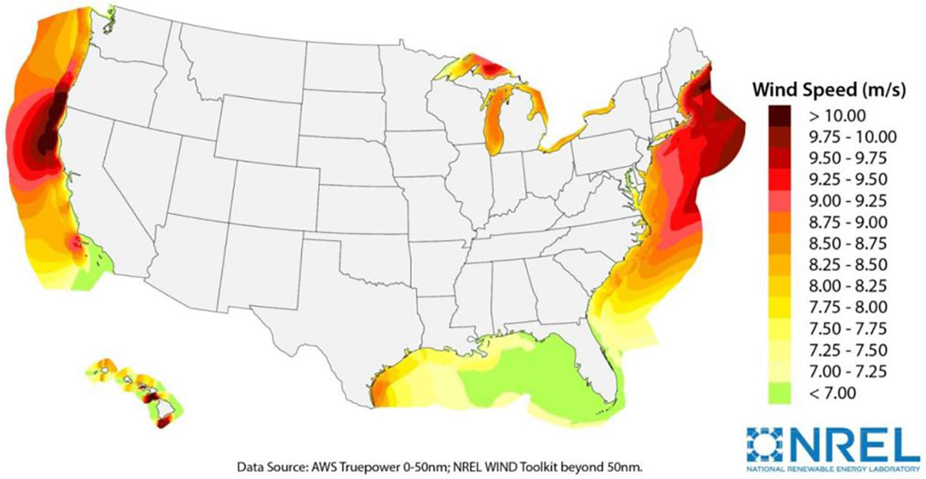
Figure 1 US annual average offshore wind speeds (Computing America’s Offshore Wind Energy Potential, https://www.energy.gov/eere/articles/computing-america-s-offshore-wind-energy-potential).
There are two components in a general optimization problem, as shown in Figure 2, an objective function and constraints. Similarly, a wind turbine layout optimization problem contains objective functions like LCOE and AEP to consider the wake effect. The constraints include the wind farm size, the turbine number, and the minimum distance according to different wake models. With all those conditions, gradient or non-gradient based algorithms could be applied to solve the optimal layout that provides the theoretical best objective value.
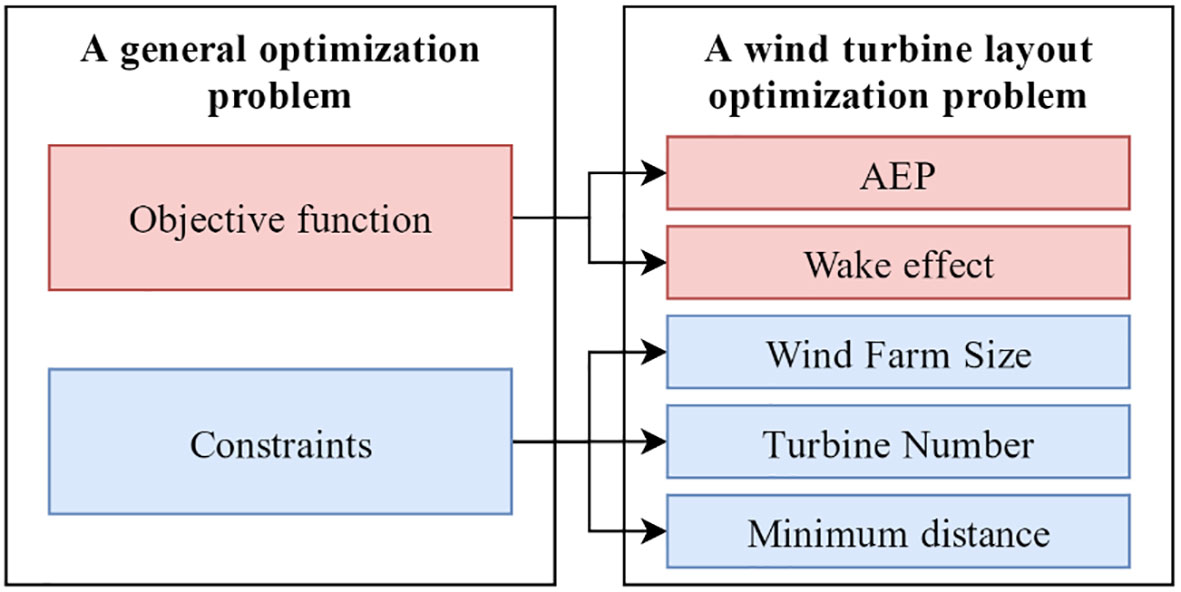
Figure 2 Components of a wind turbine layout optimization problem.
Assuming the wind farm consists of NT wind turbines, the wind farm layout is defined with the x and y coordinates of the wind turbines, i.e., X = [x1,x2,…,xN], Y = [y1,y2,…,yN]. The WFLO problem is therefore expressed as a problem of maximising or minimising an objective function f(X,Y), while subject to some constraints and requirements on the design variables. Power output, AEP, levelized cost of energy (LCOE), net present value or other financial metrics for the wind farm project are among the most often used objective functions. In this paper, the objective function is to maximise the total power output of the wind farm. Boundaries, exclusive zones, and minimum distance requirements are common constraints in the WFLO problem.
In order to compare the performance of different solutions, the objective function and constraints are treated separately. The constraint condition has priority over the objective value, and the constraint value of a potential solution is defined as:
where rϵ{1,2,⋯,R}, i,jϵ{1,2,⋯,N}, is the number of position constraints, L is the width of the wind farm, gr(z) is the constraint value between ith and jth turbines, and φ(zi) is the constraint violation value of a potential solution zi.
Numerous studies have been undertaken on multiple wind turbines’ wake effects and turbulence. Wind turbine wake effect modelling could be split into analytical models derived from empirical correlations and models based on computational fluid dynamics (CFD). CFD methods include Reynolds-Averaged-Navier-Stokes (RANS) and large eddy simulations (LES). However, CFD approaches are too computationally expensive to be used to optimize wind farm layouts. Analytical wake models are more appropriate for WFLO problems since they are less computationally expensive and WFLO demands a large number of iterations. The two most often used wake models are the Jensen wake model (Jensen, 1983; Katic et al., 1986) and the Frandsen wake model (Frandsen et al., 2006).
Recently, Bastankhah and Porté-Agel (2014) showed that a Gaussian wake model could provide substantially better results in the full-wake and partial-wake conditions (Ainslie, 1988; Bartl et al., 2012; Tian et al., 2015). Using a genetic algorithm and Gaussian wake model, Liu et al. (2021) optimized an offshore wind farm under actual seabed terrain, considering the cost of electricity. Guo et al. (2021) developed a WFLO framework considering the influence of atmosphere stability, normally neutralised by traditional studies. The Gaussian wake model is derived from equation (2), which is used to compute the normalised velocity deficit:
where σ is the standard deviation of the Gaussian-profiled velocity deficit, C(x) is the function of the downstream distance from the turbine for the velocity deficit in the centre of the wake, and r is the radial distance from the centre of the wake. C(x) can be obtained by solving the equation of mass conservation and energy conservation equation:
If the wake region is assumed to be a linear expansion, σ/d0 can be defined as:
where k*=∂σ/∂x is the growth rate and . Inserting (3) and (4) into (2), the expression for Gaussian-shaped velocity deficit is obtained as:
where y and z are spanwise and vertical coordinates, zh is the hub height of the wind turbine, γ is the yaw angle. Bastankhah and Porté-Agel (2014) also proposed the expression for ϵ:
where β is a function of the thrust coefficient CT and defined as:
Niayifar and Porté-Agel (2016) extended Equation (5) by combining the self-similar Gaussian model with a new wake superposition procedure, which guaranteed the mass and momentum conservation of the model. The results showed reasonably accurate power output prediction with the measurements and LES results. The equation used in this paper is as follows (Niayifar and Porté-Agel, 2016):
where σy and σz are standard deviations of the wake deficit in the cross-stream horizontal and vertical directions. When the wake of the upstream turbine reaches the downstream turbine, the velocity deficit varies in different positions in the area spanned by the rotor. Therefore, the integration over the rotor area A is important for the determination of the average velocity deficit Δuavg based on the following equation:
Generally, the wind speed increases with the height, and the velocity at the height z can be expressed as the power law with α = 0.14 (IEC 61400-1):
where U(z), U(zr) being the wind speed at height z and the reference wind speed at height zr respectively.
Several research works regarding the validation of the Gaussian wake model have been done. The Gaussian wake model has an acceptable agreement with high-resolution wind-tunnel measurements and the LES data (Bastankhah and Porté-Agel, 2014). Wang et al. (2022) compared field measurements with the Gaussian wake model. The result revealed that the prediction of velocity deficit and wind farm power production using the Gaussian wake model had good agreement with the field experiment. The previous validation research gives the authors confidence in choosing the Gaussian wake model to predict the AEP of a given wind farm layout.
The superposition of the wake model should be considered in a wind farm because one upstream turbine can affect more than one downstream. Numerous approaches exist in the literature for calculating the interference of many wakes. This paper uses one of the most popular methods (Katic et al., 1986). The square of the velocity deficit of a mixed wake is assumed to be the sum of velocity deficits for each wake at the calculated downstream position. The velocity of the ith turbine ui is calculated by the following equation:
where u0i and u0j are local wind speeds at ith and jth positions without placing turbines, respectively, NT is the number of turbines in the wind farm, uij is the wind speed at the wind rotor of ith turbine in the wake region of the jth turbine.
To assess the wind turbine’s energy production, the AEP is used and computed as follows:
where 8760 is the number of hours in one year, di is the wind direction, and vi is the wind speed. p(di,vi) is the joint probability of vi and di, which are obtained from the measured buoy data. E(di,vi) represents the average power production during one hour under the wind speed and wind direction, considering the wake loss.
For the Case of Maine in this paper, the objective function is set to the AEP, and the power curve of the NREL 5 MW (Jonkman et al., 2009) is applied to convert the incident wind speed to the power generated under the given wind condition.
optimization encompasses various optimization methods, each of which has strengths and weaknesses and is best suited to a particular class of optimization problems. Numerical optimization strategies, including general-purpose algorithms (such as the GA and PSO) and particularly designed algorithms, have been used in the field of the WFLO.
The GA algorithm is a gradient-free optimization method consisting of three main steps: selection, crossover and mutation. Selection is choosing and keeping a fraction that may provide superior results. Following selection, GA will carry out crossover and mutation in accordance with the associated probabilities. In order to determine the best candidates, crossover occurs at random among the chosen people. After crossing, individuals undergo mutation, which is utilised to broaden their variety in order to prevent premature convergence.
The PS algorithm is a deterministic search method, using a set pattern of search directions to locate the best placement (DuPont and Cagan, 2012). The best evaluation is kept and compared to each subsequent evaluation over the course of a pattern search, which is a direct search approach that does not need evaluating derivatives. The objective function is assessed at each potential step in the pattern and compared to the best preceding evaluation, only choosing movements that produce an increased objective value. The SA algorithm simulates the metallurgical annealing process, in which a metal’s internal energy is reduced as it is gradually cooled down by altering its internal crystal structure (Rivas et al., 2009).
The PSO algorithm is a population-based, global and stochastic optimization algorithm inspired by the social behaviour of bird flocking and fish schooling developed by Kennedy and Eberhart (1995). The PSO algorithm’s computational code is simple to construct and only requires a few input parameters. Additionally, the PSO algorithm is computationally efficient and well-suited for addressing complicated problems. GPSO was first proposed by Krohling (2004) to improve the convergence and was then applied to the WFLO by implementing the DE algorithm (Price, 2013) at the end of each iteration (Wan et al., 2012).
Another PSO-fmincon multi-stage method is also implemented to compare its performance with the proposed greedy-RS multi-stage approach. PSO is firstly adopted for the WFLO, and the optimized solution of PSO is used as the initial solution for fmincon. A gradient-based optimization tool called fmincon is also applied to case studies. Fmincon is an optimization toolbox in MATLAB which uses a finite difference method to find gradients. It is able to find a constrained or non-constrained minimum of several variables at an initial estimate. Since the fmincon is a gradient-based method, it has a relatively strong local search ability (the ability to find local optimal solutions). In this paper, the ‘interior-point’ is chosen as the algorithm in the fimincon toolbox, and the finite difference type is set to ‘forward’ to estimate gradients.
Table 1 shows the characteristics of nine optimization methods used in the case study.

Table 1 Nine optimization methods implemented in the case study.
The effectiveness of using the greedy algorithm in solving WFLO has been validated in previous studies (Chen et al., 2013; Chen et al., 2016). This paper selects the greedy algorithm as the first-stage method. The steps of the greedy algorithm are listed below:
1. The wind farm is organised into distinct grids, and each grid is assigned a unique number.
2. Add a turbine at the center of the empty grid cell with the best fitness value.
3. Try to place a wind turbine in each empty grid cell and calculate the fitness value.
4. Add the turbine at the centre of the grid with the best fitness value. When multiple grids with the same fitness value exist, the grid cell with the least number is picked for placement.
5. If the number of wind turbines in the domain is identical to the specified number, the greedy algorithm will terminate. Otherwise, it will return to step 3 and continue the procedure.
According to the greedy algorithm developed in the previous study (Chen et al., 2013), the greedy algorithm contains the locating and adjusting stage. It is shown that the adjusting stage improves the optimized result a little with a lot of computational costs. Since the greedy algorithm is not a population-based optimization method, the cost of the greedy algorithm is much smaller. Therefore, the greedy algorithm only considers the locating strategy in this paper since the discrete grid stage aims to provide a ‘near-optimal’ solution with fewer computational costs.
For the next stage, the meta-heuristic RS algorithm is chosen. The RS algorithm was first introduced by Feng and Shen (2015), and RS algorithm is easy and effective to implement by using a large amount of randomness to escape the optimal local solution and search for the optimal global solution. The basic idea of the RS algorithm is to randomly choose and move a wind turbine from its position to a new position iteratively. The new positions are accepted if the moves lead to better fitness values. Otherwise, the new positions are rejected. Details and pseudo code of the RS algorithm are referred to in the reference (Feng and Shen, 2015). The main disadvantage of the RS algorithm is its performance in the initial search stage due to its randomness. However, the greedy algorithm can provide a relatively good solution with only a few computational costs, accelerating the RS algorithm’s speed. Figure 3 shows the flowchart of the proposed multi-stage method.
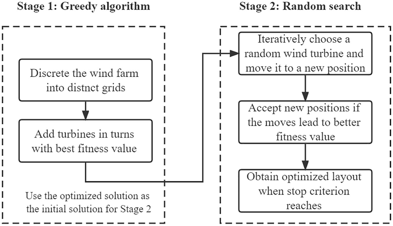
Figure 3 Flowchart of the proposed multi-stage method.
In order to verify the effectiveness of the proposed algorithm, three cases are investigated and compared with the previous studies (Grady et al., 2005; Parada et al., 2017). The characteristics of Grady’s study are as follows:
Case 1 A constant wind speed with a single incident wind direction.
Case 2 A constant wind speed with variable wind directions.
Case 3 Various wind speeds and wind directions.
Case 4 Windfarm layout optimization at the Gulf of Maine using real measured data.
Case 1, Case 2 and Case 3 are compared with Grady’s and Parada’s results, and Case 4 is the potential wind farm located in the Gulf of Maine. The wind farm size in Case 1 to Case 3 is 2000 m × 2000 m, the rotor diameter of the wind turbine is 40 m, and the hub height is 60 m. The details of each scenario are described in each subsection.
In Grady’s research, the Jensen model is applied to model the wake loss, and the wind farm is divided into 10 × 10 discrete grids (cell width of 200 m). The wind turbines are only allowed to move in the center of the grid, and a binary-coded genetic algorithm is used to solve the optimization problem. The Gaussian-based wake model (GWM) is a function of the downstream distance, hub height, and radial distance. Parada applies the GWM to the simulation, and the GWM is used to calculate the wake loss in this paper. The number of wind turbines in Case 1 is set to 30. Compared with previous studies on the discretisation of the wind farm, all optimization methods except the greedy algorithm used in this paper are implemented to optimize turbines’ positions in continuous search space. Since the wind turbines are only placed at the centre of the grid for the discrete method, the effective domain of the wind farm is 1800 m × 1800 m. Therefore, the computational domain is set to 1800 m × 1800 m so that the optimization can be compared with previous studies using the discrete method. Parada uses a more refined grid (20 ×20), but the actual computational domain is enlarged to 1900 m × 1900 m. For Case 1 to Case 3, the power generation of one turbine is calculated by the following equation (Grady et al., 2005; Mittal, 2010):
Wind farm efficiency is defined as:
where P0 is the ideal power generation without wake loss.
100 independent runs are performed for each algorithm except for the fmincon. The fimincon runs with 200 different initial schemes because it is a gradient-based algorithm and might fall into local optimal solutions. Table 2 shows the comparison results of maximum optimization solutions with previous studies. Figure 4 presents the boxplot of power efficiency of different algorithms, and Figure 5 compares the best layout schemes by different optimization algorithms. The whisker length of the boxplot in this paper is specified as 1.5 times the interquartile range. And quantile values are defined as 25th and 75th percentiles of the data.
Table 2 Comparison of global best solutions of different algorithms.
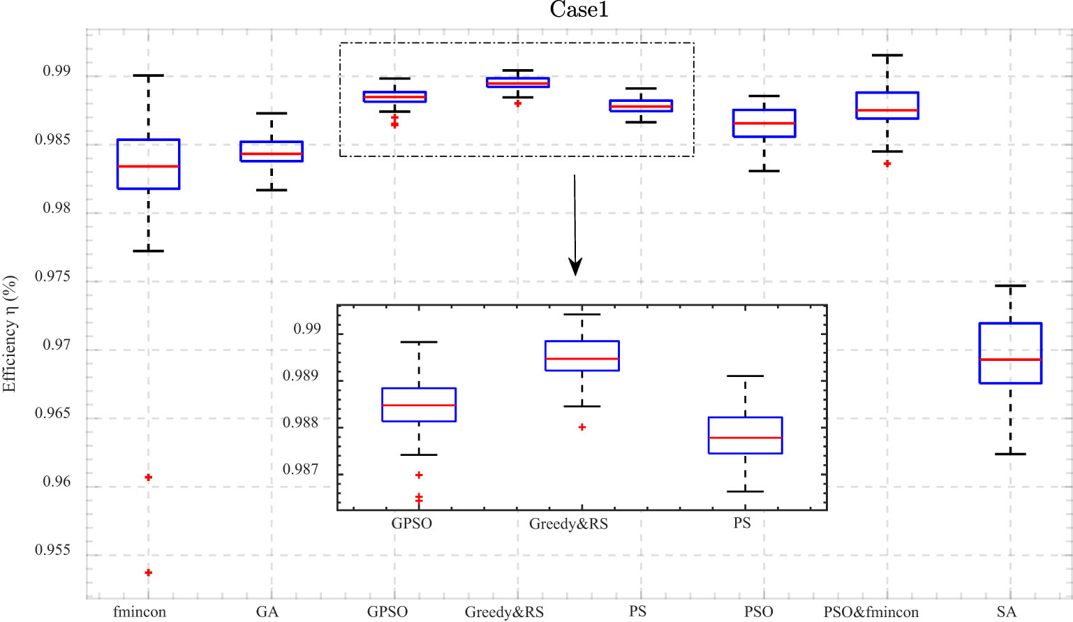
Figure 4 Boxplot of wind farm efficiency using different optimization methods.
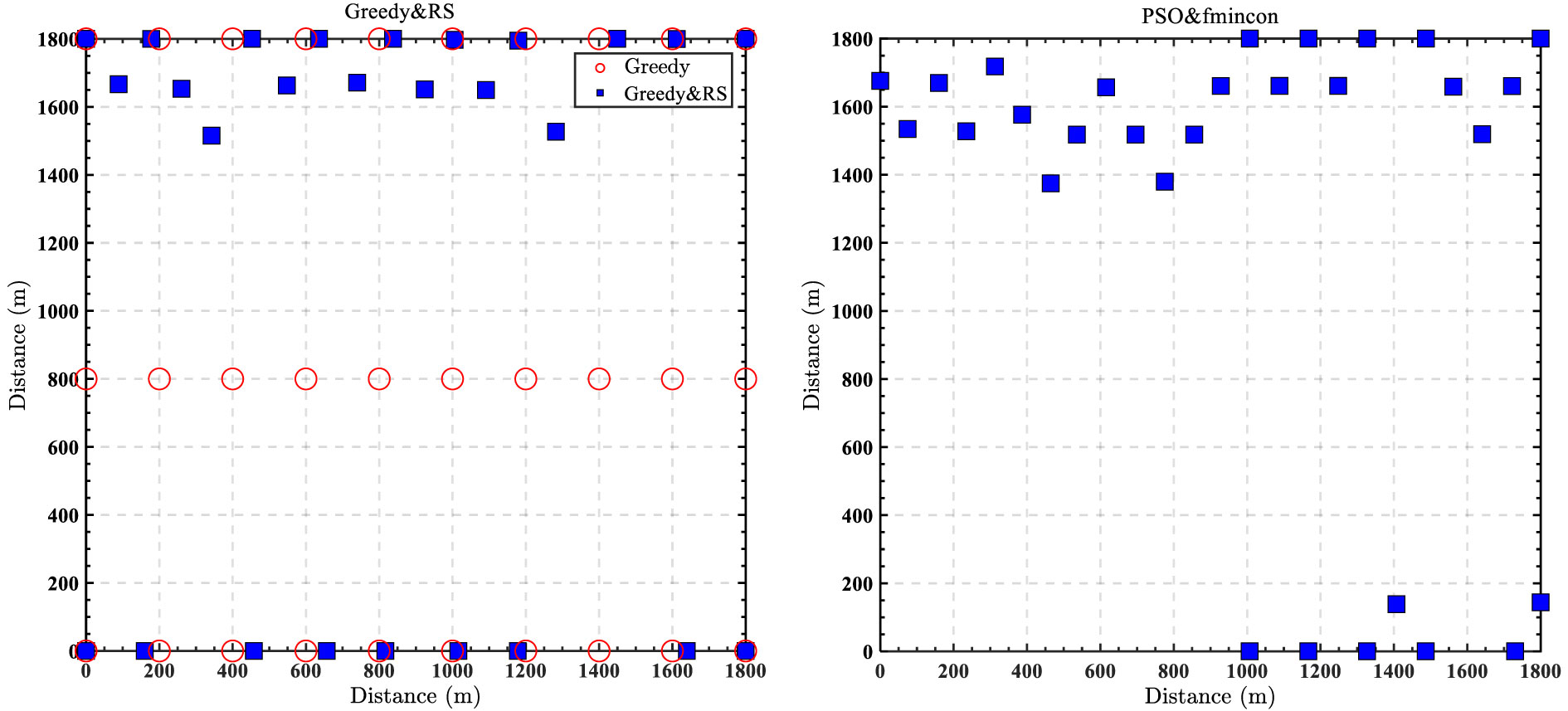
Figure 5 Comparison of optimization results of different algorithms for Case 1.
Grady and Parada obtain the same wind farm layout scheme using the GA algorithm with 10 × 10 grids but different wake models. It should be noted that the values shown in Table 2 are calculated by using the Jensen wake model. It shows that the layout evaluated by GWM obtains a higher power than the Jensen wake model. This is mainly because the velocity deficit recovers faster in the wake region when using GWM in this case. The boxplot indicates that the multi-stage method of PSO and fmincon has the best performance for Case 1, and the layout with 4.29% more power is obtained than solutions generated by discrete GA and greedy algorithms. However, the standard deviation (low variance in the results of different runs) of the PSO-fmincon multi-stage method is not the best among all algorithms, which shows that the results of the hybrid optimization are inconsistent. The power output of the proposed greedy-RS method has the highest average value with a relatively small deviation among all optimization methods. This might be due to the randomness of the RS algorithm so that the proposed method is likely to find the global optimal solution. GPSO and PS also have relatively good performance with a small standard deviation. Although fmincon has a fast convergence speed, fmincon is one of the two worst methods because it is a gradient-based method and relies on the quality of the starting solutions so that it may fall into a local maximum. Therefore, diverse initial solutions are necessary for gradient-based methods like fmincon.
Figure 5 demonstrates that the layout solutions generated by discrete GA and greedy algorithms tend to locate turbines evenly within the domain of the wind farm. On the other hand, the layout solutions obtained by the continuous scheme seem to locate turbines at the boundary of the wind farm terrain.
Case 2 is a more complicated scenario with 36 evenly distributed wind directions, and the wind speed is 12 m/s. The number of turbines is set to 39 to compare with the results of previous studies. Figure 6 presents the boxplot of different algorithms’ results, indicating that fmincon is unsuitable for the Case 2 scenario. This is primarily because the objective function of Case 2 is more sophisticated so that the gradient-based fmincon is unable to obtain the optimal global solution, and the result of fmincon is sensitive to the initial solution. It also demonstrates that the PSO-fmincon multi-stage can hardly improve the result of the PSO, which indicates that optimal solutions of the PSO reach the optimal local solution while gradient-based methods like fmincon are unable to jump out of the local best value. The multi-stage greedy-RS still performs best considering the optimal solutions and standard deviation, followed by PS and GPSO. GA, SA, and fmincon are the top three worst algorithms in Case 2. The greedy algorithm used in the first stage provides a relatively good solution for the second stage, which leads to the phenomenon that the power output of the worst optimal solution from the greedy-RS is higher than the average power outputs of other algorithms.
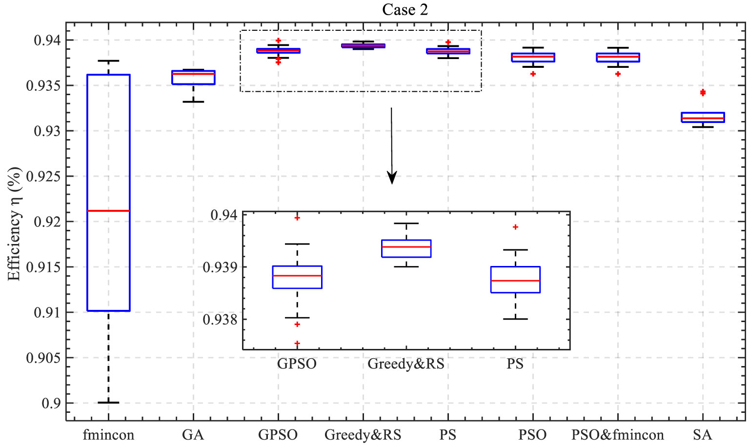
Figure 6 Boxplot of wind farm efficiency using different optimization methods.
Table 3 presents the global best solutions using different methods, and it indicates that GPSO, greedy-RS, and PS obtain 2.22% higher power output than Grady’s study and 0.62% more than Parada’s result. Figure 7 compares the wind farm layout using proposed methods and previous studies’ results. Major optimized solutions tend to locate turbines in the outmost zone of the computational domain. In contrast, the results obtained from fmincon and SA have more turbines located in the central area of the wind farm.
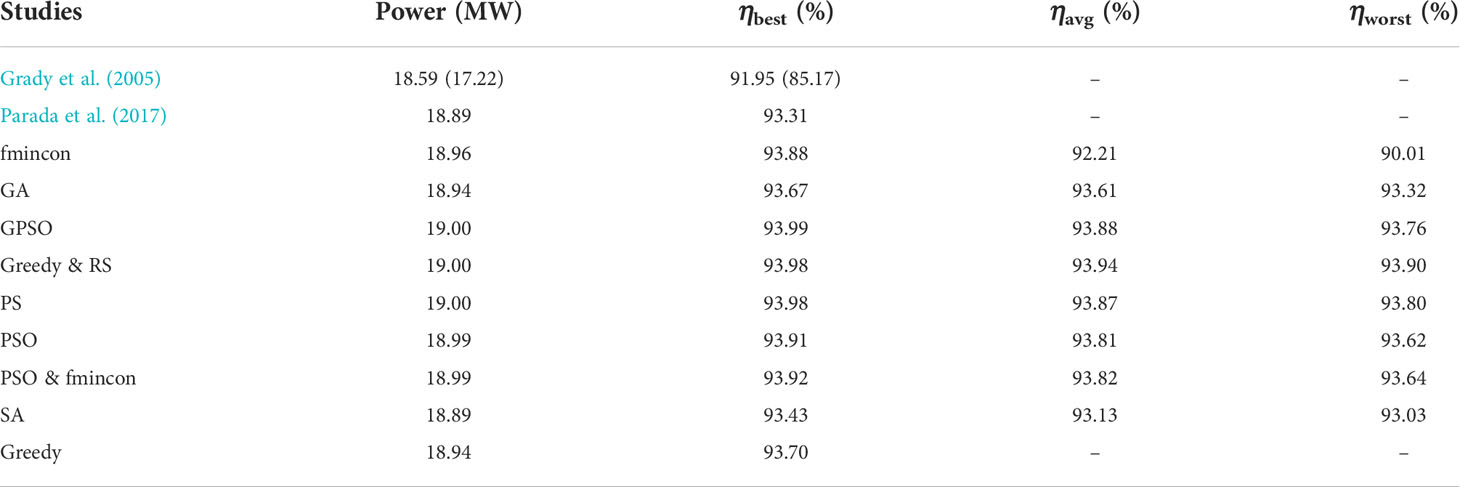
Table 3 Comparison of global best solutions of different algorithms.
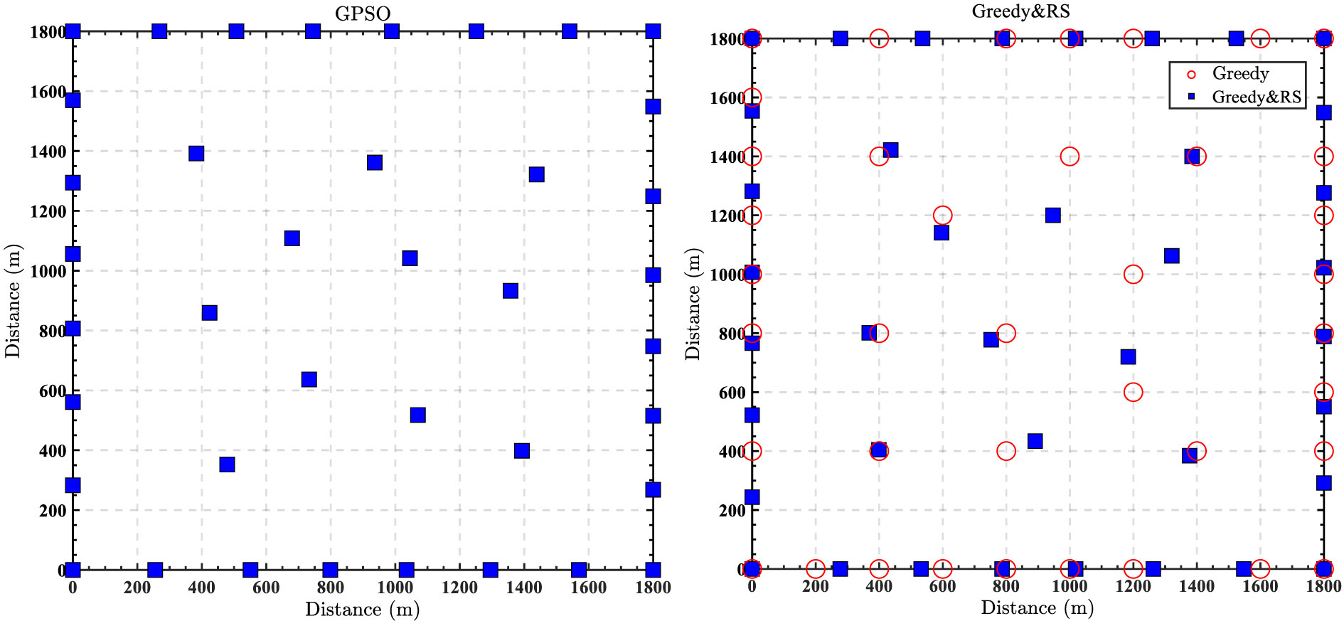
Figure 7 Comparison of optimization results of different algorithms for Case 2.
Case 3 has variable wind speeds and wind directions. The number of wind turbines in Case 3 is identical to that in Case 2. In Case 3, the wind speeds of 12 m/s and 17 m/s are predominant, especially between 280° and 360°, as shown in Figure 8. Figure 9 presents the boxplot of the results of different algorithms, and the optimization result is similar to the one obtained in Case 2. Greedy-RS, PS, and GPSO remain the top three best methods in handling Case 3 scenarios. The difference in power output increment of the greedy-RS is more obvious in Case 3, which reveals the robustness of the proposed multi-stage. Due to the multiple wind speeds and wind directions, the complexity of the optimization problems increases and the advantage of the greedy-RS is prominent in Case 3.

Figure 8 Wind rose for Case 3.
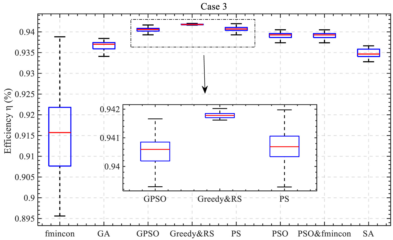
Figure 9 Boxplot of wind farm efficiency using different optimization methods.
Table 4 compares the global best solutions of different algorithms and shows that the high complexity of the wind scenario leads to more minor improvements in power output than in previous studies. The wind farm efficiency of PS improves by 1.01% higher power output than Grady’s study and 0.62% than Parada’s result. Figure 10 compares the wind farm layout using proposed methods and previous studies’ results. It can be seen that layouts generated by greedy-RS have approximately 82% of turbines located in the outermost area of the wind farm, while layouts generated by PS and GPSO have approximately 74% and 71% of turbines located in the outermost zone.
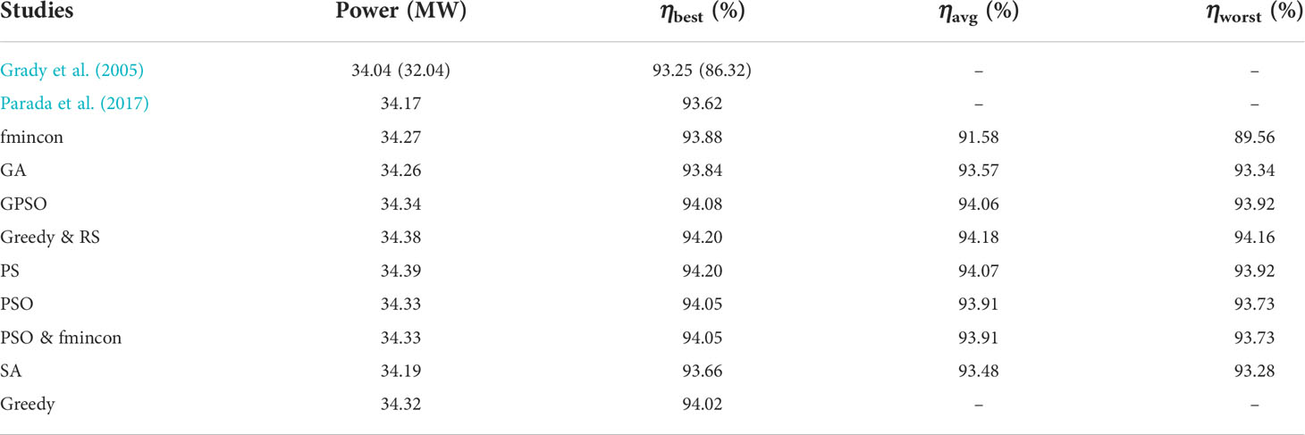
Table 4 Comparison of global best solutions of different algorithms.
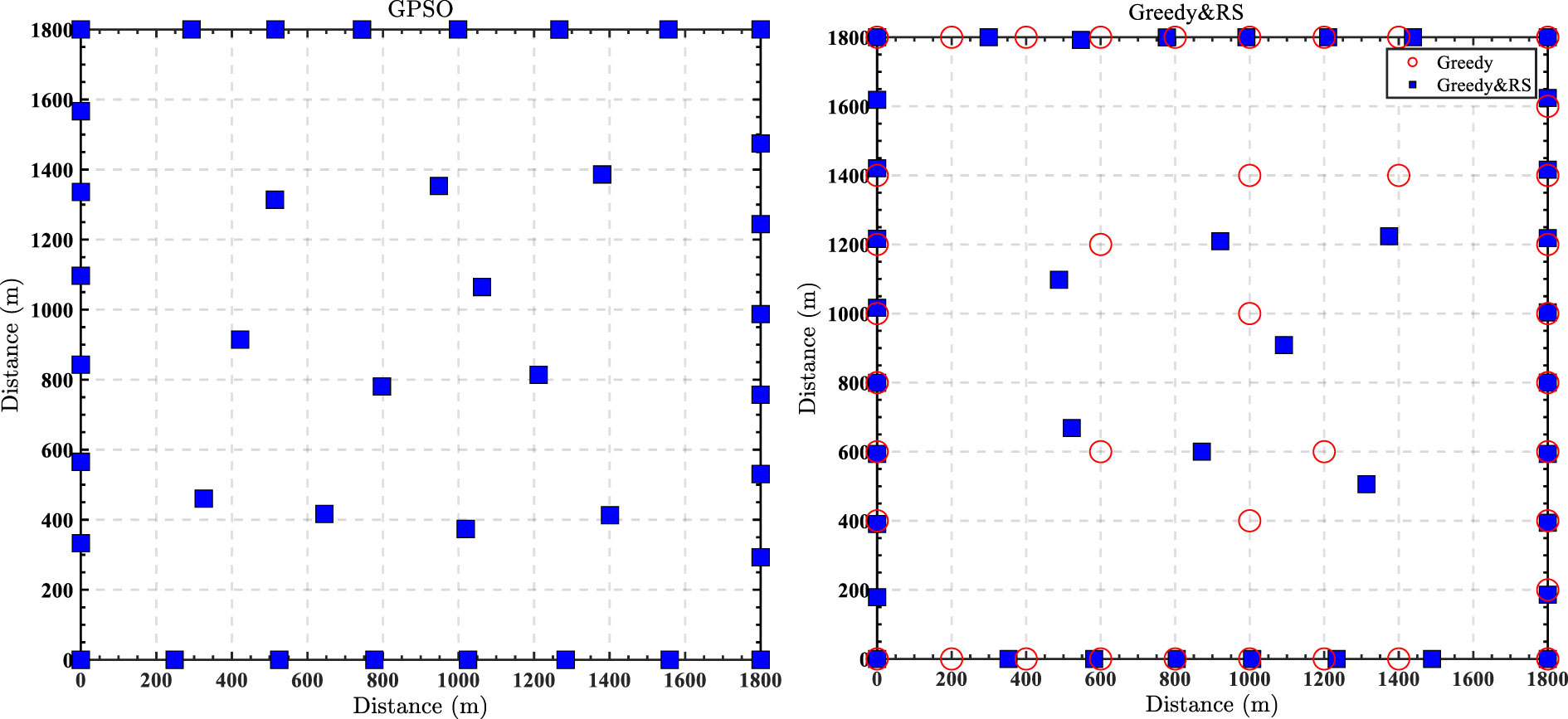
Figure 10 Comparison of optimization results of different algorithms for Case 2.
The proposed offshore wind farm in the Gulf of Maine and the location of the Gulf of Maine is shown in Figure 11. The site is on the Northeast coast of the United States and the southeast coast of Canada, whose north latitude is 43.72 and west longitude is 69.33. The Gulf of Maine contains considerable offshore wind power potential. New England Aqua Ventus I, the first commercial floating wind project in the US, was set up in the Gulf of Maine. The wind farm covers an area of 28.00 km2 (5.93 km × 5.93 km) and consists of 46 wind turbines. Figure 12 shows the wind rose plot obtaining data from Buoy E01 (NERACOOS, https://www.neracoos.org/) from January 2003 to December 2018.
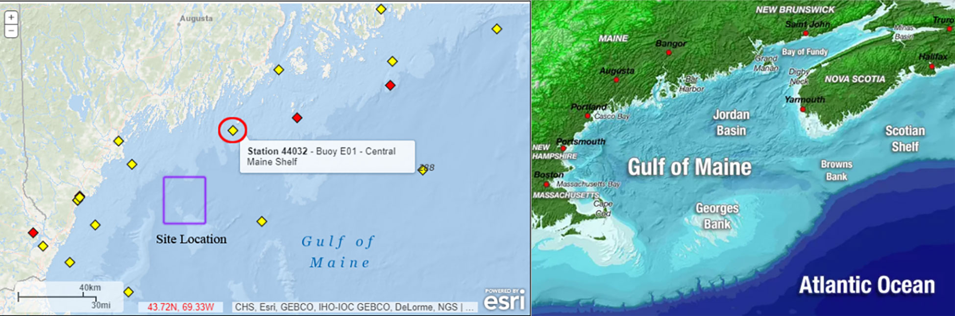
Figure 11 Proposed location of the offshore wind farm (left) and the location of the Gulf of Maine (right). https://www.noaa.gov/, https://www.tradeonlytoday.com/environmental-issues/study-finds-gulf-of-maine-is-getting-warmer).
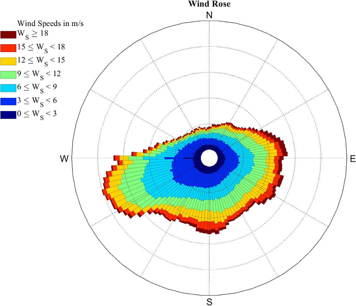
Figure 12 Wind rose used to present wind climatology at the Gulf of Maine.
The target turbine model of the wind farm is the NREL 5 MW wind turbine, and Table 5 presents the parameters of the 5 MW wind turbine. The power curve is applied to compute the power generation at a given wind speed (Jonkman et al., 2009).
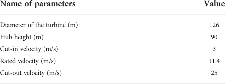
Table 5 Parameters of the 5 MW wind turbine.
Figure 13 presents the boxplot of wind farm efficiency using different optimization methods. The first notable result is that the optimal result of SA becomes quite unstable as fmincon. As expected from the previous three cases, greedy-RS, PS, and GPSO are still the top three methods in optimising Case Maine. Table 6 compares optimal solutions of different algorithms, and it is apparent that the discrete greedy algorithm has the fastest convergence speed with a relatively good optimal result. Only greedy-RS and PS have average fitness values of over 926 GW, and the time cost of PS is slightly better than greedy-RS. The average best AEP enhancement of the greedy-RS method is evident compared with other optimization methods. The second-stage RS algorithm shows the effectiveness of searching the global optimal solution if a relatively good initial solution is provided by the greedy algorithm.
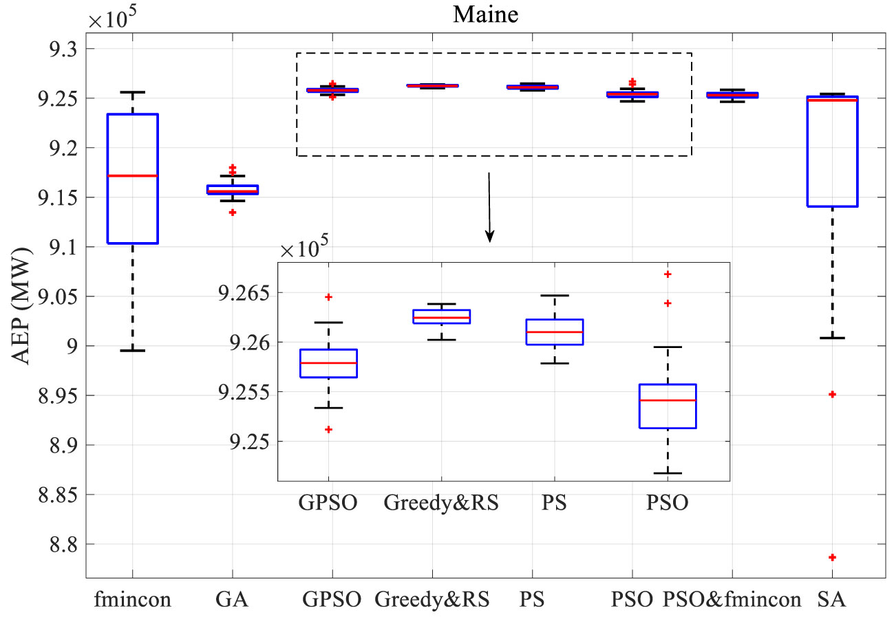
Figure 13 Boxplot of wind farm AEP using different optimization methods.
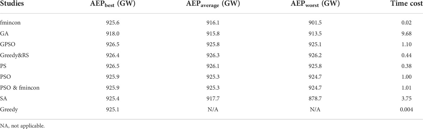
Table 6 Comparison of optimal solutions of different algorithms.
It should be noted that the time considered in this paper is the CPU time of running optimizations on a desktop with the 3.8 GHz Ryzen 9 3900x and 32 GB of RAM. The time cost of all algorithms is normalised by the computational time of the PSO. Figure 14 presents the time cost versus AEP with different optimization methods. It indicates that the greedy algorithm and fmincon have the fastest convergence speed. The greedy-RS multi-stage approach and PS have the top two performances concerning optimal solutions and time costs, followed by GPSO and PSO. Figure 15 compares the optimization results of different algorithms for Case Maine. The layouts still seem to be irregular and scattered, and approximately 60% of the wind turbines are placed in the outermost domain of the wind farm.
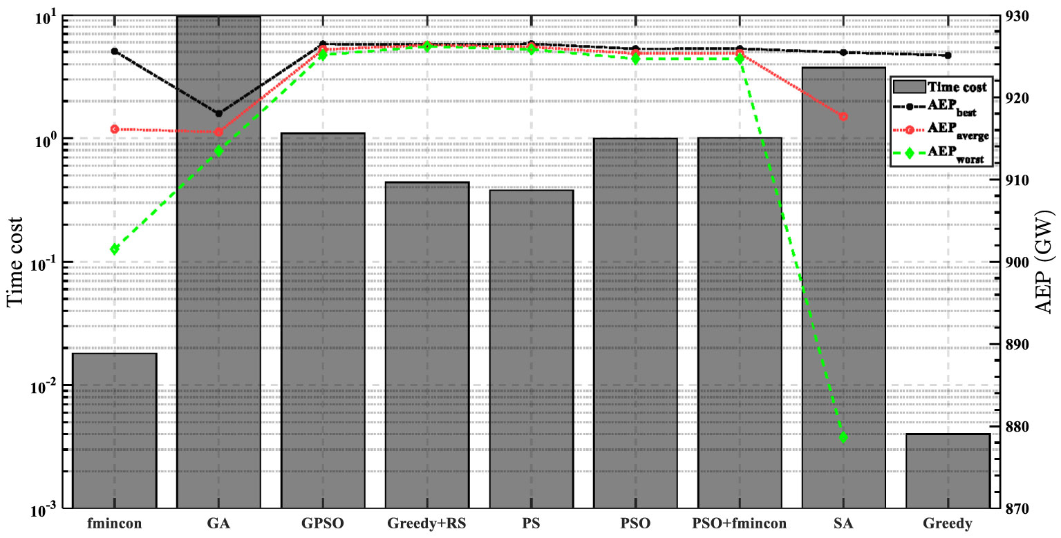
Figure 14 Time cost versus AEP with different optimization methods.
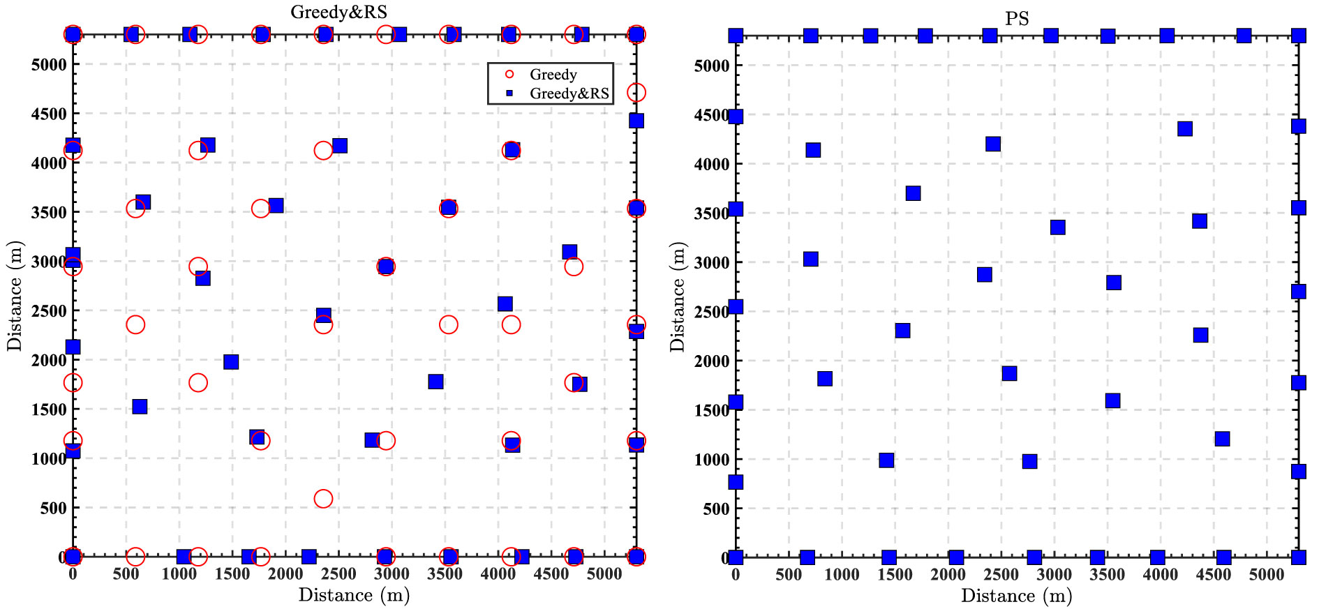
Figure 15 Comparison of optimization results of different algorithms for Case Maine.
This paper proposes a new multi-stage approach by combining both discrete and continuous schemes, maximising the advantages and bypassing disadvantages of individual algorithms for different stage’s purposes. The first stage’s goal is to obtain a good initialised solution for the following optimization with small computational costs. Therefore, the discrete greedy algorithm is ideal in the first stage since it is less computationally expensive than population-based methods like PSO. In the second stage, RS is preferred due to its outstanding performance in finding globally optimal solutions, which has been proven in previous studies (Feng and Shen, 2015; Brogna et al., 2020). The main disadvantage of RS, however, is the relatively expensive computational cost at the first stage because the feasible region is too large to research randomly. In this case, the greedy algorithm becomes a remedy of RS in solving WFLO.
To demonstrate the effectiveness of the greedy-RS multi-stage approach, a comparative analysis of optimization methods is conducted by studying three typical wind cases and one potential wind farm case. The results show that greedy-RS has good robustness regarding the low standard deviations and computational costs. It also indicates that fmincon is not ideal at the second stage because it is a gradient-based method, and local optimization results will be easily obtained. Continuous search space gives rise to a more efficient wind farm than a discrete computational domain. GPSO presents relatively good and stable results compared with PSO, but the robustness of GPSO is still inferior to the greedy-RS multi-stage approach.
In summary, a new multi-stage approach is presented, and a systematical study of different optimizations provides references for selecting proper algorithms in WFLO. The developed multi-stage RS method shows promising results, which provides valuable insight into selecting appropriate optimization methods in the WFLO. Further work will thoroughly test the robustness of the proposed method by implementing different wake models and considering more real-life wind farm projects. More test cases will be carried out to consider errors in the AEP estimation introduced by different fidelities wake models and the potential errors in the wind climate.
The raw data supporting the conclusions of this article will be made available by the authors, without undue reservation.
All authors contributed to conception and design of the study. XX and LD developed the models necessary for the study. XX and LD performed the analyzes and made the results. XX, LD, YX, and OG wrote the first draft of the manuscript. JG, ZZ, and PD supervised the work. All authors reviewed and edited the manuscript. All authors contributed to the article and approved the submitted version.
The authors gratefully acknowledge the financial support from the National Natural Science Foundation of China [Grant No. 51909109; Grant No. 52101314] and the Natural Science Foundation of Jiangsu Province [Grant No. BK20190967]. The authors also gratefully acknowledge the support from the Natural Science Foundation of the Jiangsu High Education Institutions [Grant No. 19KJB580010] and the Scientific Research Foundation of Jiangsu University of Science and Technology.
The authors declare that the research was conducted in the absence of any commercial or financial relationships that could be construed as a potential conflict of interest.
All claims expressed in this article are solely those of the authors and do not necessarily represent those of their affiliated organizations, or those of the publisher, the editors and the reviewers. Any product that may be evaluated in this article, or claim that may be made by its manufacturer, is not guaranteed or endorsed by the publisher.
Ainslie J. F. (1988). Calculating the flowfield in the wake of wind turbines. J. Wind Eng. Ind. Aerodyn. 27 (1-3), 213–224. doi: 10.1016/0167-6105(88)90037-2
Bai F., Ju X., Wang S., Zhou W., Liu F. (2022). Wind farm layout optimization using adaptive evolutionary algorithm with Monte Carlo tree search reinforcement learning. Energy Convers. Manage. 252, 115047. doi: 10.1016/j.enconman.2021.115047
Bartl J., Pierella F., Sætrana L. (2012). Wake measurements behind an array of two model wind turbines. Energy Proc. 24, 305–312. doi: 10.1016/j.egypro.2012.06.113
Bastankhah M., Porté-Agel F. (2014). A new analytical model for wind-turbine wakes. Renewable Energy 70, 116–123. doi: 10.1016/j.renene.2014.01.002
Brogna R., Feng J., Sørensen J. N., Shen W. Z., Porté-Agel F. (2020). A new wake model and comparison of eight algorithms for layout optimization of wind farms in complex terrain. Appl. Energy 259, 114189. doi: 10.1016/j.apenergy.2019.114189
Cazzaro D., Trivella A., Corman F., Pisinger D. (2022). Multi-scale optimization of the design of offshore wind farms. Appl. Energy 314, 118830. doi: 10.1016/j.apenergy.2022.118830
Chen K., Song M. X., He Z. Y., Zhang X. (2013). Wind turbine positioning optimization of wind farm using greedy algorithm. J. Renewable Sustain. Energy 5 (2), 023128. doi: 10.1063/1.4800194
Chen K., Song M. X., Zhang X., Wang S. F. (2016). Wind turbine layout optimization with multiple hub height wind turbines using greedy algorithm. Renewable Energy 96, 676–686. doi: 10.1016/j.renene.2016.05.018
Computing America’s Offshore Wind Energy Potential. Available at: https://www.energy.gov/eere/articles/computing-america-s-offshore-wind-energy-potential.
Croonenbroeck C., Hennecke D. (2021). A comparison of optimizers in a unified standard for optimization on wind farm layout optimization. Energy 216, 119244. doi: 10.1016/j.energy.2020.119244
DuPont B. L., Cagan J. (2012). An extended pattern search approach to wind farm layout optimization. ASME. J. Mech. Des. 134 (8), 081002. doi: 10.1115/1.4006997
DuPont B., Cagan J., Moriarty P. (2016). An advanced modeling system for optimization of wind farm layout and wind turbine sizing using a multi-level extended pattern search algorithm. Energy 106, 802–814. doi: 10.1016/j.energy.2015.12.033
Eroğlu Y., Seçkiner S. U. (2012). Design of wind farm layout using ant colony algorithm. Renewable Energy 44, 53–62. doi: 10.1016/j.renene.2011.12.013
Feng J., Shen W. Z. (2015). Solving the wind farm layout optimization problem using random search algorithm. Renewable Energy 78, 182–192. doi: 10.1016/j.renene.2015.01.005
Frandsen S., Barthelmie R., Pryor S., Rathmann O., Larsen S., Højstrup J., et al. (2006). Analytical modelling of wind speed deficit in large offshore wind farms. Wind Energy 9 (1-2), 39–53. doi: 10.1002/we.189
Grady S. A., Hussaini M. Y., Abdullah M. M (2005). Placement of wind turbines using genetic algorithms. Renewable energy. 30 (2), 259-270.
Guo N., Zhang M., Li B., Cheng Y. (2021). Influence of atmospheric stability on wind farm layout optimization based on an improved Gaussian wake model. J. Wind Eng. Ind. Aerodyn. 211, 104548. doi: 10.1016/j.jweia.2021.104548
Jensen N. O. (1983). A note on wind generator interaction (Roskilde, Denmark: Risø National Laboratory).
Jiang D., Peng C., Fan Z., Chen Y., Cai X. (2013). “Modified binary differential evolution for solving wind farm layout optimization problems,” in 2013 IEEE Symposium on Computational Intelligence for Engineering Solutions. 23–28 (IEEE).
Jonkman J., Butterfield S., Musial W., Scott G. (2009). Definition of a 5-MW reference wind turbine for offshore system development (Golden, CO (United States: National Renewable Energy Lab). No. NREL/TP-500-38060.
Katic I., Højstrup J., Jensen N. O. (1986). “A simple model for cluster efficiency,” in European wind energy association conference and exhibition, Vol. 1. 407–410. Rome, Italy: A. Raguzzi.
Kennedy J., Eberhart R. (1995). “Particle swarm optimization,” in Proceedings of ICNN’95-International Conference on Neural Networks, Vol. 4. 1942–1948 (IEEE).
Krohling R. A. (2004). “Gaussian Swarm: a novel particle swarm optimization algorithm,” in IEEE Conference on Cybernetics and Intelligent Systems, 2004, Vol. 1. 372–376) (IEEE).
Liu Z., Fan S., Wang Y., Peng J. (2021). Genetic-algorithm-based layout optimization of an offshore wind farm under real seabed terrain encountering an engineering cost model. Energy Convers. Manage. 245, 114610. doi: 10.1016/j.enconman.2021.114610
Marmidis G., Lazarou S., Pyrgioti E. (2008). Optimal placement of wind turbines in a wind park using Monte Carlo simulation. Renewable Energy 33 (7), 1455–1460. doi: 10.1016/j.renene.2007.09.004
Mittal A. (2010). Optimization of the layout of large wind farms using a genetic algorithm (Case Western Reserve University, United States). Available at: http://rave.ohiolink.edu/etdc/view?acc_num=case1270056861.
Mosetti G., Poloni C., Diviacco B. (1994). Optimization of wind turbine positioning in large wind farms by means of a genetic algorithm. J. Wind Eng. Ind. Aerodyn. 51 (1), 105–116. doi: 10.1016/0167-6105(94)90080-9
NERACOOS. Available at: https://mariners.neracoos.org/platform/E01%20-%2044032.
Niayifar A., Porté-Agel F. (2016). Analytical modeling of wind farms: A new approach for power prediction. Energies 9 (9), 741. doi: 10.3390/en9090741
Parada L., Herrera C., Flores P., Parada V. (2017). Wind farm layout optimization using a Gaussian-based wake model. Renewable energy 107, 531–541. doi: 10.1016/j.renene.2017.02.017
Price K. V. (2013). “Differential evolution,” in Handbook of optimization (Berlin, Heidelberg: Springer), 187–214.
Renkema D. J. (2007). Validation of wind turbine wake models: Using wind farm data and wind tunnel measurements.
Rivas R. A., Clausen J., Hansen K. S., Jensen L. E. (2009). Solving the turbine positioning problem for large offshore wind farms by simulated annealing. Wind Eng. 33 (3), 287–297. doi: 10.1260/0309-524X.33.3.287
Song M., Chen K., Wang J. (2018). Three-dimensional wind turbine positioning using Gaussian particle swarm optimization with differential evolution. J. Wind Eng. Ind. Aerodyn. 172, 317–324. doi: 10.1016/j.jweia.2017.10.032
Song M., Chen K., Wang J. (2020). A two-level approach for three-dimensional micro-siting optimization of large-scale wind farms. Energy 190, 116340. doi: 10.1016/j.energy.2019.116340
Tian L., Zhu W., Shen W., Zhao N., Shen Z. (2015). Development and validation of a new two-dimensional wake model for wind turbine wakes. J. Wind Eng. Ind. Aerodyn. 137, 90–99. doi: 10.1016/j.jweia.2014.12.001
Wang Y., Kamada Y., Maeda T., Xu J., Zhou S., Zhang F., et al. (2022). Diagonal inflow effect on the wake characteristics of a horizontal axis wind turbine with Gaussian model and field measurements. Energy 238, 121692. doi: 10.1016/j.energy.2021.121692
Wan C., Wang J., Yang G., Gu H., Zhang X. (2012). Wind farm micro-siting by Gaussian particle swarm optimization with local search strategy. Renewable Energy 48, 276–286. doi: 10.1016/j.renene.2012.04.052
Wen Y., Song M., Wang J. (2022). Wind farm layout optimization with uncertain wind condition. Energy Convers. Manage. 256, 115347. doi: 10.1016/j.enconman.2022.115347
Wu Y. K., Wu W. C., Zeng J. J. (2019). Key issues on the design of an offshore wind farm layout and its equivalent model. Appl. Sci. 9 (9), 1911. doi: 10.3390/app9091911
Wu Y., Xia T., Wang Y., Zhang H., Feng X., Song X., et al. (2022). A synchronisation methodology for 3D offshore wind farm layout optimization with multi-type wind turbines and obstacle-avoiding cable network. Renewable Energy 185, 302–320. doi: 10.1016/j.renene.2021.12.057
Xu X., Gaidai O., Naess A., Sahoo P. (2020). Extreme loads analysis of a site-specific semi-submersible type wind turbine. Ships Offshore Struct. 15 (sup1), S46–S54. doi: 10.1080/17445302.2020.1733315
Xu X., Wang F., Gaidai O., Naess A., Xing Y., Wang J. (2022a). Bivariate statistics of floating offshore wind turbine dynamic response under operational conditions. Ocean Eng. 257, 111657. doi: 10.1016/j.oceaneng.2022.111657
Xu X., Xing Y., Gaidai O., Wang K., Patel K. S., Dou P., Zhang Z.. (2022b). A novel multi-dimensional reliability approach for floating wind turbines under power production conditions. Front. Mar. Sci., 1412. doi: 10.3389/fmars.2022.970081
Keywords: gaussian-based wake model, wind farm layout optimization, multi-stage approach, hybrid optimization methods, offshore wind
Citation: Xu X, Du L, Zhang Z, Gu J, Xing Y, Gaidai O and Dou P (2022) A case study of offshore wind turbine positioning optimization methodology using a novel multi-stage approach. Front. Mar. Sci. 9:1028732. doi: 10.3389/fmars.2022.1028732
Received: 26 August 2022; Accepted: 27 October 2022;
Published: 11 November 2022.
Edited by:
Zhiming Yuan, University of Strathclyde, United KingdomReviewed by:
Sebastian Solari, Universidad de la República, UruguayCopyright © 2022 Xu, Du, Zhang, Gu, Xing, Gaidai and Dou. This is an open-access article distributed under the terms of the Creative Commons Attribution License (CC BY). The use, distribution or reproduction in other forums is permitted, provided the original author(s) and the copyright owner(s) are credited and that the original publication in this journal is cited, in accordance with accepted academic practice. No use, distribution or reproduction is permitted which does not comply with these terms.
*Correspondence: Lin Du, ZHVsaW4yOTI5QDEyNi5jb20=
Disclaimer: All claims expressed in this article are solely those of the authors and do not necessarily represent those of their affiliated organizations, or those of the publisher, the editors and the reviewers. Any product that may be evaluated in this article or claim that may be made by its manufacturer is not guaranteed or endorsed by the publisher.
Research integrity at Frontiers
Learn more about the work of our research integrity team to safeguard the quality of each article we publish.