The oxygen minimum zone relative depth is a key driver of dolphin habitats in the northern Humboldt Current System

Highly mobile odontocetes need habitats with environmental conditions with the potential of aggregating enough and high-quality prey, to maximize foraging success. Until now, the characterization of those habitats was in terms of physical and biological indicators of high production, capable of attracting and sustaining prey. Nevertheless, there has been no approach to quantifying the effects of a biophysical characteristic of the ocean with proven effects on the vertical distribution of prey for cetaceans: The oxygen minimum zone (OMZ) depth. In the northern branch of the Humboldt Current System off Peru (~6-18° S), a shallow OMZ (30-50 m) affects the distribution of the Peruvian anchovy (Engraulis ringens), main prey for several marine predators, including dolphins. We hypothesized these predators would aggregate in productive areas, but with preference for places where the relative OMZ depth can constrain prey vertically, making it more accessible and maximizing foraging success. We fitted Bayesian habitat models for three dominant odontocete species in this region, with multiple combinations of environmental covariates, smoothing techniques, and temporal and spatial random effects. Cetacean data came from 23 dedicated surveys spanning 2001-2019. Habitat predictors included the spatial anomalies of sea surface temperature, surface chlorophyl-a, pycnocline depth and OMZ depth. Dusky (Lagenorhynchus obscurus) and common dolphins (Delphinus delphis) preferred productive, cold areas with a very shallow OMZ, regardless of the season, while bottlenose dolphins (Tursiops truncatus) aggregated in both cold and warm waters, also with shallow OMZ. The former two species of higher metabolic demands would maximize energy intake by selecting areas with highly aggregated prey, while the latter, of more moderate metabolic needs and more diverse prey, would exploit less restricted habitats.

1. Introduction

Predators must make foraging decisions based on fluctuations of prey in space and time (Stephens, 2008). These fluctuations are often related to changes in the environment that trigger or deplete biological production, modulating prey availability (Redfern et al., 2006). Marine predators such as seabirds and cetaceans tend to occupy diverse types of habitats according to specific needs (Ballance et al., 1997; Manocci et al., 2014). Red-footed boobies (Sula sula), wedge-tailed shearwaters (Ardenna pacifica) (Ballance et al., 1997), common dolphins (Delphinus delphis spp), harbor porpoises (Phocoena phocoena), and minke whales (Balaenoptera acutorostrata) (Spitz et al., 2012), occupy intense productivity areas where prey is abundant and highly caloric. In contrast, species such as sooty terns (Onychoprion fuscatus) (Ballance et al., 1997), pygmy sperm whales (Kogia breviceps), Cuvier’s beaked whales (Ziphius cavirostris), or sperm whales (Physeter macrocephalus) (Spitz et al., 2012), may occur in more oligotrophic areas, where they feed on less caloric and more intermittent prey.

However, although prey abundance is an important aspect, prey accessibility could also play a relevant role in areas selected by predators. In the northern Humboldt Current System (NHCS), the depth of prey aggregations explained better the areas with high seabird diving probability than only the their size (Boyd et al., 2015). Likewise, in South Georgia, king penguins (Aptenodytes patagonicus) forage in areas with predictably dense fish schools but also occurring at shallow depths (Proud et al., 2021). Physical barriers such as water-column stratification associated to deep thermoclines restricts prey to upper layers, making it more accessible for predators (Ropert-Coudert et al., 2009; Kokubun et al., 2010; Meyer et al., 2020).

The NHCS exhibits the oxygen minimum zone (OMZ) restricts oxygenated coastal waters to depths shallower than 100 m (Fuenzalida et al., 2009). This region is dominated by the biogeographical zone known as the Humboldt Province (~6-18° S; Ibanez-Erquiaga et al., 2018), where a rapid vertical decrease in dissolved oxygen usually occurs at ~25-50 m depth, from surface concentrations of ~6 ml l^-1 to hypoxic conditions of <1 ml l^-1 (Graco et al., 2017). Contrary to physical barriers, these low concentrations constrain vertically the epipelagic species at a physiological level, since they can tolerate only moderate to high dissolved oxygen concentrations, such as the Peruvian anchovy (Engraulis ringens) (Bertrand et al., 2008; Bertrand et al., 2011), which is the preferred prey for local seabird and sealion populations (Soto et al., 2006; Barbraud et al., 2018).

The OMZ depth fluctuates seasonally (Passuni et al., 2016; Graco et al., 2017) and interannually (Espinoza-Morriberón et al., 2019) in the NHCS. It is very shallow during summer and early autumn (up to 20 m), less so during spring (~20-40 m), and deeper in winter (~50 m) (Passuni et al., 2016; Graco et al., 2017). Although this seasonality could be partially correlated to that of the pycnocline at local scales (e.g., Bertrand et al., 2014), this is unclear for the entire region. Local respiration, vertical mixing/stratification, and mesoscale circulation can modulate the OMZ (Thomsen et al., 2016; Vergara et al., 2016). Interannually, El Niño Southern Oscillation forces OMZ depth fluctuations, deepening it below 100 m and displacing it ~60 km offshore during warm El Niño events; and shoaling it up to 10 m during cold La Niña events (Graco et al., 2007; Gutiérrez et al., 2008; Gutiérrez et al., 2016; Graco et al., 2017; Mogollón and Calil, 2017).

Global warming affects dissolved oxygen in the ocean due to lower solubility at higher temperatures (Oschlies et al., 2018; Limburg et al., 2020). Consequences include OMZ shoaling in the northeast Atlantic Ocean, reducing the vertical habitat for tropical pelagic fishes such as billfishes (Order: Istiophoriformes) and tunas, and their prey (Prince and Goodyear, 2006; Stramma et al., 2012). Since future scenarios of OMZ shoaling remain unclear for the NHCS, it is relevant to understand its role in the current distribution of marine apex predators for taking timely management and conservation decisions.

In the NHCS, dusky (Lagenorhynchus obscurus), common (Delphinus delphis), and bottlenose (Tursiops truncatus) dolphins are dominant predators. The first two have high energy demands (Mckinnon, 1994; Spitz et al., 2012), feed mainly on high caloric prey (Spitz et al., 2010), and conform large pods, from hundreds to thousands of individuals (Van Waerebeek and Würsig, 2018; Perrin, 2018). In the analogous upwelling ecosystem of the California Current, common dolphins also exhibit the largest biomass and highest prey consumption among cetaceans (Barlow et al., 2008). In contrast, bottlenose dolphins present more moderate metabolic costs (Spitz et al., 2012). In the NHCS, diets of common and dusky dolphins are based mainly on anchovies, an abundant high-quality energy prey; while bottlenose dolphins prefer lower energy prey such as myctophids, mackerels, and opportunistically, anchovies and sardines (Mckinnon, 1994; García-Godos et al., 2007). Our aim was to evaluate analytically the potential importance of the OMZ depth for these species’ distributions and habitat suitability, in agreement with their different requirements, already described. We hypothesized that these predators would prefer productive areas with spatially shallower OMZ, which would constrain prey vertically, and that these distributions would vary strongly at the seasonal scale.

2. Methods

2.1. Cetacean data

We recorded sightings of delphinid species from 2001 to 2019 during 23 dedicated scientific surveys for stock assessment of Peruvian anchovy (Engraulis ringens) by Instituto del Mar del Perú (IMARPE), throughout Peruvian territorial waters. Overall, cruises were conducted twice a year: February to April and August to October, but also included July, November, and December. In summary, here were three surveys in the austral hemisphere’s winter, six in spring, eight in summer, and six in autumn. Surveys consisted of parallel cross-shore transects of ∼185 km long and ∼27.8 km of parallel separation between them (Supplementary Material, Appendix 1, Figure A.1). Sampling effort summed 59,874 km; 4,950 km in winter; 18,383 km in spring; 19,421 in summer; and 17,120 km in autumn (Supplementary Material, Appendix 1, Figure A.1). Navigation was at a constant speed of ~10 knots.

One or two observers equipped with 10x50 hand-held binoculars scanned visually the water surface from the top of the vessel’s bow (i.e. 12.3 m above the sea level in the R/V Humboldt and 5.1 m in the R/V Olaya), within a semicircular area of 180° in front of the vessel. Searching effort was conducted during daylight hours only (~6:00-18:00 h), with pauses at 7:00-8:00 h and 12:00-14:00 h, and only when weather conditions were ideal (i.e., Beaufort < 3). GPS coordinates were taken automatically each 1.8 km or every six minutes, and used to obtain on-effort small transects of similar lengths (7 to 8 km; Supplementary Material, Appendix 1, Figure A.2). Each cetacean sighting was then assigned to its closest transect in time and space, along with the species identity and group size. Only sightings of common dolphins (213 groups; 12,239 individuals), dusky dolphins (403 groups; 10,455 individuals), and offshore-ecotype bottlenose dolphins (hereafter, bottlenose dolphins) (222 groups; 8,653 individuals) were analyzed, although all cetacean species were recorded during navigation. The inshore-ecotype bottlenose dolphin was not included since they only inhabit very shallow coastal waters in this region (within one kilometer offshore; Van Waerebeek et al., 1990), which were not covered by our surveys due to navigation constraints.

2.2. Habitat predictors

Dynamic oceanographic variables are important descriptors for understating marine mammal distributions through bottom-up processes. We used some of those described in previous studies as potential indicators of habitat suitability for cetaceans (e.g., Ballance et al., 2006; Forney et al., 2012; Roberts et al., 2016). We excluded the use physiographic variables since our study aimed to the comprehension of dynamic habitats.

2.2.1. Oxygen minimum zone depth

During the same scientific surveys described above, vertical profiles were cast at stations every ~2-4 hours of navigation. A total of 3,191 profiles of dissolved oxygen concentration were used to estimate the depth at which such concentration drops to 2 ml l^-1 for each profile, which we interpreted in this study as the oxygen minimum zone depth. This threshold was chosen because it limits the physiology and therefore vertical distribution of epipelagic prey species for dolphins, such as the Peruvian anchovy (Vaquer-Sunyer and Duarte, 2008; Ekau et al., 2010; Bertrand et al., 2011).

We used oxygen concentrations estimated with the Winkler method at fixed depths of 0, 10, 25, and 50 m, spanning 2001-2005, from the World Ocean Database (Garcia et al., 2010). The rest of the data (2007-2019) consisted of Conductivity-Temperature-Depth-Oxygen (CTDO) casts from the surface to 500 m, provided by IMARPE (www.gob.pe/imarpe). Winkler test for dissolved oxygen were also used to verify the accuracy of CTDO readings (IMARPE, unpublished data). CTDO data were smoothed as 9-m depth running means to avoid noise from the original depth resolution of each cast. Only casts with more than 13 casts were selected.

Given the horizontal sparsity of these OMZ depths, it was not possible to pair the nearest values to each transect of cetacean survey effort. First, we had to build a continuous layer of predicted OMZ depth values for each survey within the study area. For this, we fitted a Bayesian regression model of the OMZ depth (OMZD) as a function of a spatial autocorrelation random effect (W), applying stochastic partial differential equations (SPDE), and a second-order random walk effect (u) of the horizontal distance to the coast (DC) (Supplementary Material, Appendix 2). The former was approximated by a Gaussian Markov Random Field (GMRF) (Zuur et al., 2017). This procedure involves dividing the study area into an irregular spatial mesh called the Delaunay triangulation, created from the geographic coordinates of the observations (Supplementary Material, Appendix 2, Figure A2.1). This allows for predictions in non-sampled sites, accounting for the explicit spatial structure. Equation 1 shows the main regression and the parameters’ likelihoods (intercept and residuals are omitted):

$${\mu }_{OMZDi}=uD{C}_i + W_i$$

$$OMZ{D}_i\sim \log N({\mu }_{OMZDi},{{\sigma }^2}_{OMZD}), i=1,\dots ,n$$

$$uD{C}_i-2uD{C}_{i-1}+uD{C}_{i-2} \sim N(0,{\sigma }_u^2), i=2,\dots ,n$$

$\begin{array}{ll}{W}_i \sim N(0,\Sigma )& \text{[Eq. 1]}\end{array}$

Where Σ is a covariance matrix quantified through the Matérn correlation function (Zuur et al., 2017). Default Gamma distributions were used as vague priors for unknown parameters given the absence of previous information for them. This analysis followed the integrated nested Laplace approximation (INLA) (Rue et al., 2009), implemented by the R-INLA package (Rue et al., 2009) in R (R Core Team, 2021). The final OMZD layers had a 0.1° resolution, and each pixel was paired to the nearest transect from the same survey.

2.2.2. Pycnocline depth

We used 1,745 vertical profiles of conductivity, temperature, and depth (CTD) collected during cetacean surveys to estimate the pycnocline depth (PD), since a shallow pycnocline is typically associated to productive regions and potential prey aggregation for cetaceans (e.g., Reilly, 1990; Scott et al., 2012). Prior to the pycnocline depth estimation, the vertical array of CTD values were smoothed for each cast to avoid noise, through 9-m running means. Then, we calculated the Brunt-Väisälä frequency (cycles h^-1) for each depth to measure the degree of stratification, using the gsw package (Kelley et al., 2017) within R. The PD was the depth with the maximum Brunt-Väisälä frequency in each cast. Finally, we modeled a continuous spatial layer of the variable for each survey, following the same INLA procedure described above for the OMZ depth (Subsection 2.2.1; Equation 1). The final layer of PD also had a 0.1° resolution and transects were paired to the nearest pixel from the same survey.

2.2.3. Sea surface temperature

Remotely sensed sea surface temperature (SST) data were obtained from the National Oceanic and Atmospheric Administration (NOAA), through the AVHRR Pathfinder Version 5.2 (PFV52) database, at a daily 0.04° cell resolution (https://www.ncei.noaa.gov/products/avhrr-pathfinder-sst; Saha et al., 2018). We only used data of quality level >3 according to both criteria provided by the database’s metadata. We estimated a mean values per pixel spanning the duration of the survey and scaled the variable to a 0.1° resolution pixels, which were then paired to the nearest survey transect from the same survey.

2.2.4. Chlorophyll-a

Remotely sensed sea surface chlorophyll-a concentration (CHL) was obtained from two sources, with 8-day, 9-km original resolution: (i) NOAA’s ERDDAP (https://coastwatch.pfeg.noaa.gov/erddap/) database from the SeaWiFS sensor (1997-2002), and (ii) the Ocean Color website (http://oceancolor.gsfc.nasa.gov) database, derived from the Aqua-MODIS sensor (2002-2019). We estimated means for the duration of each survey and the variable was produced at 0.1° resolution, for pairing pixels to the closest transect of the same survey.

2.2.5. Spatial anomalies of dynamic variables

Considering that dolphin species in our study area occur year-round, it is likely their distributions and aggregations are driven by the spatial environmental variability regardless of time. To partially remove variations in time of each of the dynamic variables described in sections 2.2.1 to 2.2.4, we subtracted the mean value of the study area to each pixel at any given time or survey, generating new predictors which we named for this study ‘spatial anomalies’ (i.e. OMZD_A, PD_A, SST_A, and CHL_A), which would maximize the horizontal structure and gradients (Supplementary Material, Appendix 3, Figures A.3.1–A.3.3). Thus, negative values of SST_A and CHL_A represent colder and more productive sites than the rest of the study area, while positive values, the opposite. Likewise, negative values of OMZD_A and PD_A represented shallower OMZ and pycnocline relative to the study area, whilst positive values, the contrary. Finally, these new derived variables were additional predictors within the different competing models.

2.2.6. Interannual variations

El Niño Southern Oscillation (ENSO) affects the western and eastern tropical Pacific, especially along the equator and off Ecuador and Peru (Wang and Fiedler, 2006). Coastal local effects of exceptional intense warming are called “coastal El Niño” and can occur despite the absence of high temperature anomalies in the central equatorial Pacific (Takahashi and Martínez, 2017, Echevin et al., 2018). We included this scale of environmental variability using the El Niño Coastal Index (ICEN). It is based on temperature anomalies in the Niño 1 + 2 region (90°W-80°W, 10°S-0°) which extent from 3 to 10° S and categorizes interannual scenarios of different intensity: La Niña strong, moderate, and weak conditions (< -1.4 to -1), neutral conditions (-1 to 0.4), El Niño weak, moderate, strong, and extreme conditions (0.4 to > 3) (Takahashi et al., 2014).

2.3. Habitat suitability models

INLA framework was also used to model dolphin groups (g) at each transect (i) as a function of several (k) combinations of the environmental predictors (X) described above. We assessed collinearity and correlation among variables through the variance inflation vector (VIF) and Pearson’s correlation, using the R packages usdm (Naimi et al., 2014) and the Performance Analytics (Peterson and Carl, 2020). Competing models included only uncorrelated variables (r < 0.5) (Supplementary Material, Appendix 4, Figure A.4). It is important to point out that the available amount of data for pycnocline estimations was lower than that used for OMZ depth. We also tested for Poisson, negative binomial, and zero-inflated Poisson likelihood functions for the response variable, as well as incremental complexity of polynomials (β), as smoothing techniques, for each predictor and/or combinations of them. These included the additive and multiplicative effects of covariate pairs (e.g., SST_A-OMZD_A, CHL_A-OMZD_A, SST_A-PD_A, and CHL_A-PD_A).

Following the spatial techniques explained above for the OMZ depth and the pycnocline depth layer estimations, we included a spatial autocorrelation random effect (W) (Supplementary Material, Appendix 5, Figure A.5) to account for the evident lack of independency among transects. For each species, we also tested the effect of the seasonal variability as a cyclic random effect (θ) of the season of the year (S; winter, spring, summer, and autumn), as well as the interannual effect (φ) of ICEN:

$\begin{array}{ll}{\mu }_{gi=}\left[{\displaystyle \sum _{{}_{k=1}^{j=1}}^{{}_{k=nc}^{j=ns}}{\beta }_j·X_{k,i}}\right]+W_i+\theta ·S_i+\phi ·ICE{N}_i,\mathrm{\hspace{0.17em} }i=1,\dots ,n& \text{[Eq. 2]}\end{array}$

Since there was some heterogeneity of the survey effort among transects, and dolphin group sizes were highly variable among groups, we included an offset variable (E) that balanced the response variable as a known component of the animal count likelihood’s mean. This would produce predictions in terms of encounter rates of animals, instead of group counts, even if the main response variable of the model was the latter (e.g., Cañadas et al., 2002):

$\begin{array}{ll}{E}_i=\frac{\left(\widehat{L}·L_i\right)}{Ln\left(\widehat{S}\right)·\left(Ln\left(S_i/g_i\right)+1.1\right)}& \text{[Eq. 3]}\end{array}$

$$\widehat{L}=\frac{{\sum }^{ }{L}_i}{n_{L_i}}$$

$$\widehat{S}=\frac{{\sum }^{ }{S}_i}{n_{gi}}$$

Where $\widehat{L}$ represent the mean transect length, $\widehat{S}$ the mean group size and g_i the number of groups in each transect. Natural logarithm was used to maintain homogeneous quantities considering the high variability of group sizes. Default Gamma distributions were used as vague priors for all unknown parameters.

The best model among competing structures was chosen according to the lowest value of the Watanabe Akaike Information Criterion (WAIC), checking also for the Conditional Predictive Ordinate (CPO) to assure a good fit. We scaled predictions to values from 0 to 1, since we interpreted them as an index of habitat suitability, potential for the aggregation of each dolphin species. We also used the position of dolphin sightings without available environmental information (i.e., independent of the model) to evaluate graphically the models’ spatial predicting performance. Finally, model outputs of habitat suitability were projected onto both environmental and geographical space to infer the changes in the distribution of each species, seasonally and inter-annually, depending on the best model structure chosen. Since during the study period (2001-2019), ICEN fluctuated between -1.08 and 2.2, we projected our model results accordingly, only on three scenarios: La Niña weak conditions, El Niño strong conditions, and neutral conditions.

2.3.1. Distance to shore of the most suitable habitats

To evaluate the ocean-coast habitat extension or contraction, we estimated the mean distance to shore of all pixels whose habitat suitability predictions were > 0.7. These posterior means and their differences among seasons were estimated with a Markov Chain Monte Carlo procedure implemented in the JAGS language (Plummer, 2003). Non-informative uniform priors were used. Three chains were run in parallel with 200,000 iterations each. Ten percent were discarded as a burning phase, and only one of every 10 iterations was retained to avoid chain state autocorrelations.

3. Results

3.1. Correlated predictors

Initially, no collinearity was detected among variable pairs (VIF < 5; Supplementary Material, Appendix 4, Table A.4). However, since SST_A and CHL_A, and OMZD_A and PD_A pairs showed high correlations (r > 0.5; Supplementary Material, Appendix 4, Figure A.4), they were discarded within the same model structure.

3.2. Models selected

For all species, the response variable was best represented by a zero-inflated Poisson likelihood. CHL_A and OMZD_A were the best predictors of dusky dolphin habitat suitability, whilst SST_A and OMZD_A performed better for common and bottlenose dolphins (Table 1). Second-degree polynomials were selected as smoothers for dusky and common dolphins, and a first-degree polynomial for bottlenose dolphins. The inclusion of the seasonal effect improved the model’s performance for all species (Table 1). Nevertheless, interannual effects benefited model performance only for common and bottlenose dolphins (Table 1). The best models for each species were:

TABLE 1

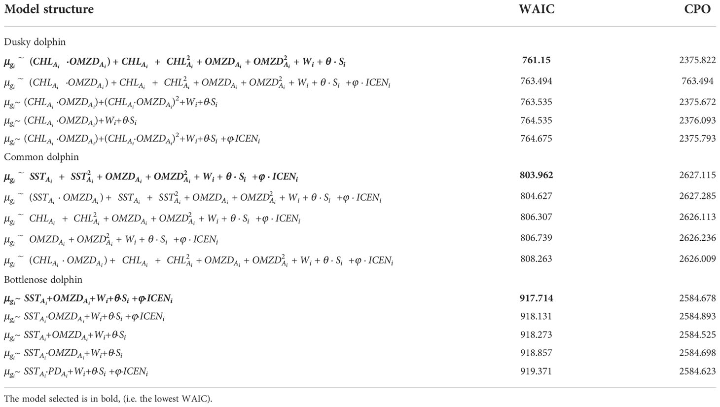
Table 1 Comparison of the best five model structures for predicting the habitat suitability of dusky, common, and bottlenose dolphins in northern Humboldt Current System.

Dusky dolphins:

$\begin{array}{ll}{\mu }_{g_i}\sim (CH{L}_{A_i} · OMZ{D}_{A_i})+CH{L}_{A_i} + CH{L}_{A_i}^2+OMZ{D}_{A_i}+OMZ{D}_{A_i}^2+W_i+\theta ·S_i& \text{[Eq. 4]}\end{array}$

Common dolphins:

$\begin{array}{ll}{\mu }_{g_i}\sim SS{T}_{A_i}+ SS{T}_{A_i}^2+OMZ{D}_{A_i}+OMZ{D}_{A_i}^2+W_i+\theta ·S_i+\phi ·ICE{N}_i& \text{[Eq. 5]}\end{array}$

Bottlenose dolphins:

$\begin{array}{ll}{\mu }_{g_i}\sim SS{T}_{A_i}+OMZ{D}_{A_i}+W_i+\theta ·S_i+\phi ·ICE{N}_i& \text{[Eq. 6]}\end{array}$

3.3. Inferred dolphin distributions

Dusky dolphins showed preferences for highly productive areas where the OMZ was spatially shallower. Highly positive CHL_A (0 to +4 mg m^-3) and negative OMZD_A (0 to -100 m) predicted the highest habitat suitability (0.7 to 1), especially during summer, autumn, and spring (Figure 1). In general, the species aggregated in the coastal zone off central and southern Peru (8-18°S) (Figure 2). During summer, the model showed an expansion to more oceanic waters (median distance to the coast: 57.6 km; 95%-CI: 54.7 – 64.6) (Supplementary Material, Appendix 6, Figure A.6.1). In contrast, during winter, the distribution was notoriously restricted to coastal waters (median: 19.4 km; 95%-CI: 13.3 – 32.2) (Supplementary Material, Appendix 6, Figure A.6.1). During autumn and spring, the distribution expanded again, with medians of 48.1 km (95%-CI: 43.7 – 53.1) and 56.5 km (95%-CI: 51.8 – 62.1) from the coast, respectively, although in a lesser extent than that of the summer (Supplementary Material, Appendix 6, Figure A.6.1). Likewise, the highest values of habitat suitability were predicted for summer, autumn, and spring (up to 1) and lower values in winter (up to 0.8) (Figure 2).

FIGURE 1

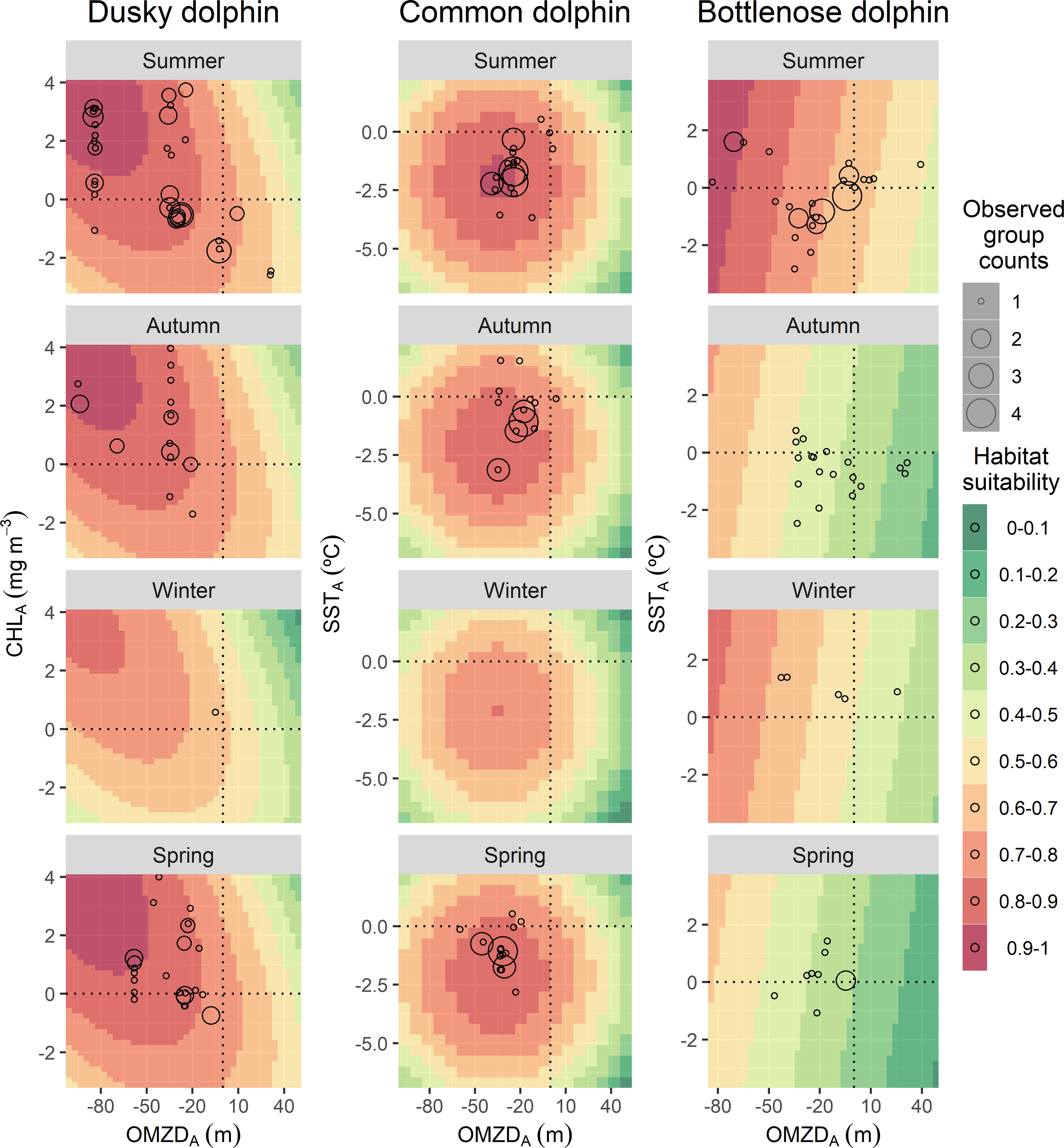
Figure 1 Predicted values of habitat suitability of dolphin species in the northern Humboldt Current System for a theoretical environmental space, based on the covariates included in the best models: the oxygen minimum zone depth spatial anomaly (OMZD_A), the remotely sensed chlorophyll-a concentration spatial anomaly (CHL_A) and the remotely sensed seas surface temperature anomaly (SST_A). Empty circle sizes represent the observed group counts in each sample unit (i.e., transect).

FIGURE 2

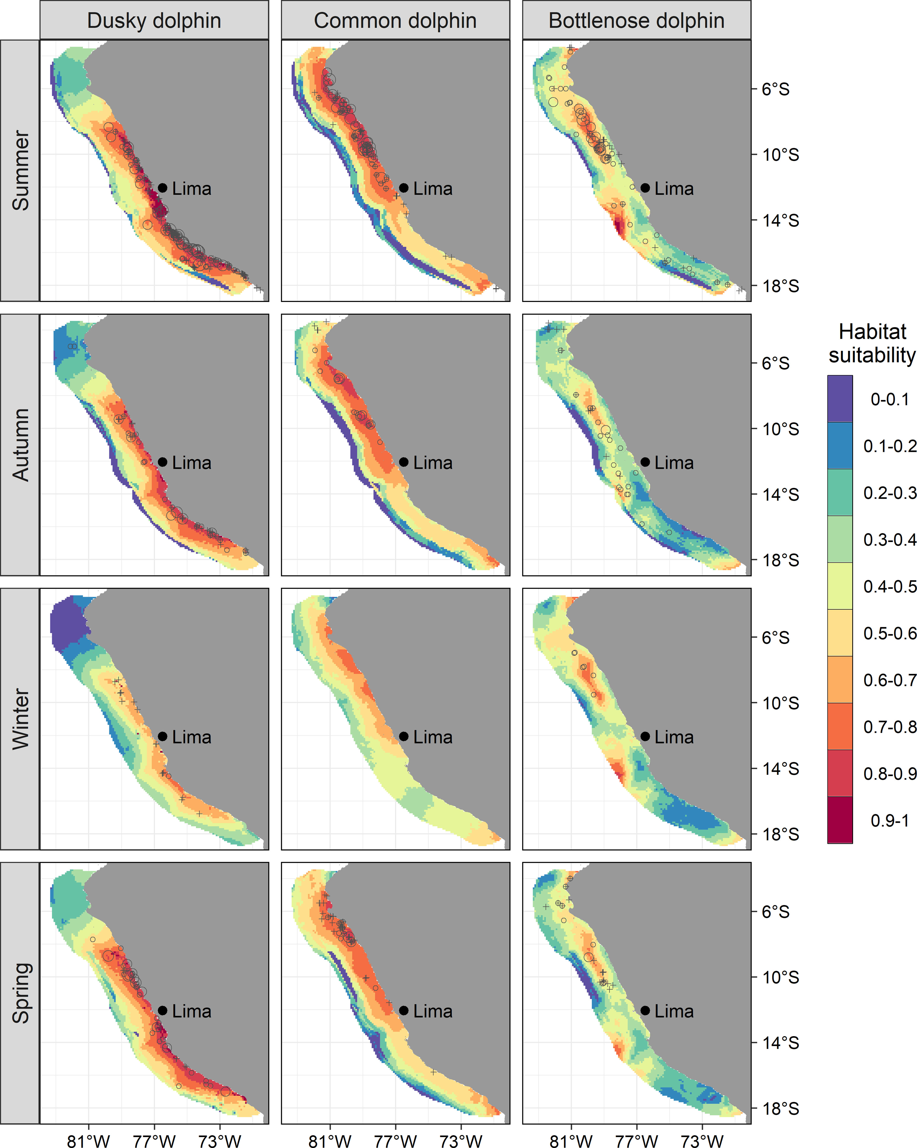
Figure 2 Predicted values habitat suitability of dolphin species in the northern Humboldt Current System for the geographical space. Empty circle sizes represent the observed group counts in each sample unit (i.e., transect). Crosses are validation data, not included in the model’s fitting.

Common dolphins showed affinity to cold waters also with very shallow OMZ. Negative values of SST_A (0 to -6 °C) and OMZD_A (0 to -100 m) predicted the highest habitat suitability (0.7 – 1) during all seasons (Figure 1). The species was mainly distributed in the coastal zone off northern-central Peru (3 - 12° S) (Figure 2). Specifically, the highest habitat suitability (0.8 - 1) were observed in two spots between 5-8° and around 10° S. Models also showed a coastal retraction of the species during winter (median: 46.8 km; 95%-CI: 34.4 – 68.2) (Supplementary Material, Appendix 6, Figure A.6.2). During summer and autumn, the distribution extended to more oceanic waters, with medians of 68 km (95%-CI: 61.9 – 75.2) and 64.9 km (95%-CI: 58.3 – 73.1), respectively (Supplementary Material, Appendix 6, Figure A.6.2). During these two seasons, the largest groups were observed, mainly at 7° S and 10° S. During spring, the species retracted again to the coast (median 57.6 km; 95%-CI: 51.3 – 65.7) (Supplementary Material, Appendix 6, Figure A.6.2) with higher habitat suitability around 7° S. The model highlights southern Peru (17 - 18° S) as a potential distribution area, although with lower values (0.7 - 0.8). Interestingly, a coastal area between 14 - 17° S presented very low habitat suitability (0.3 - 0.6), where dusky dolphins exhibited the highest. In summer and autumn, common dolphins showed the highest habitat suitability predictions (up to 1 and 0.9), while during winter and spring, they reached up to 0.8 and 0.9, respectively (Figure 2). According to ICEN’s effects, El Niño conditions triggered higher habitat suitability (up to 1) than La Niña (up to 0.9) for common dolphins. The most favorable habitat was characterized by colder waters (SST_A: 0 to -6 °C) and shallower OMZD (0 to -90 m) during both interannual conditions (Figure 3). Spatially, this pattern suggested a higher degree of the species aggregation and wider coverage during warm years, at ~6 and between 7 and 11°S, while lower habitat suitability persisted off southern Peru (Figure 5).

FIGURE 3

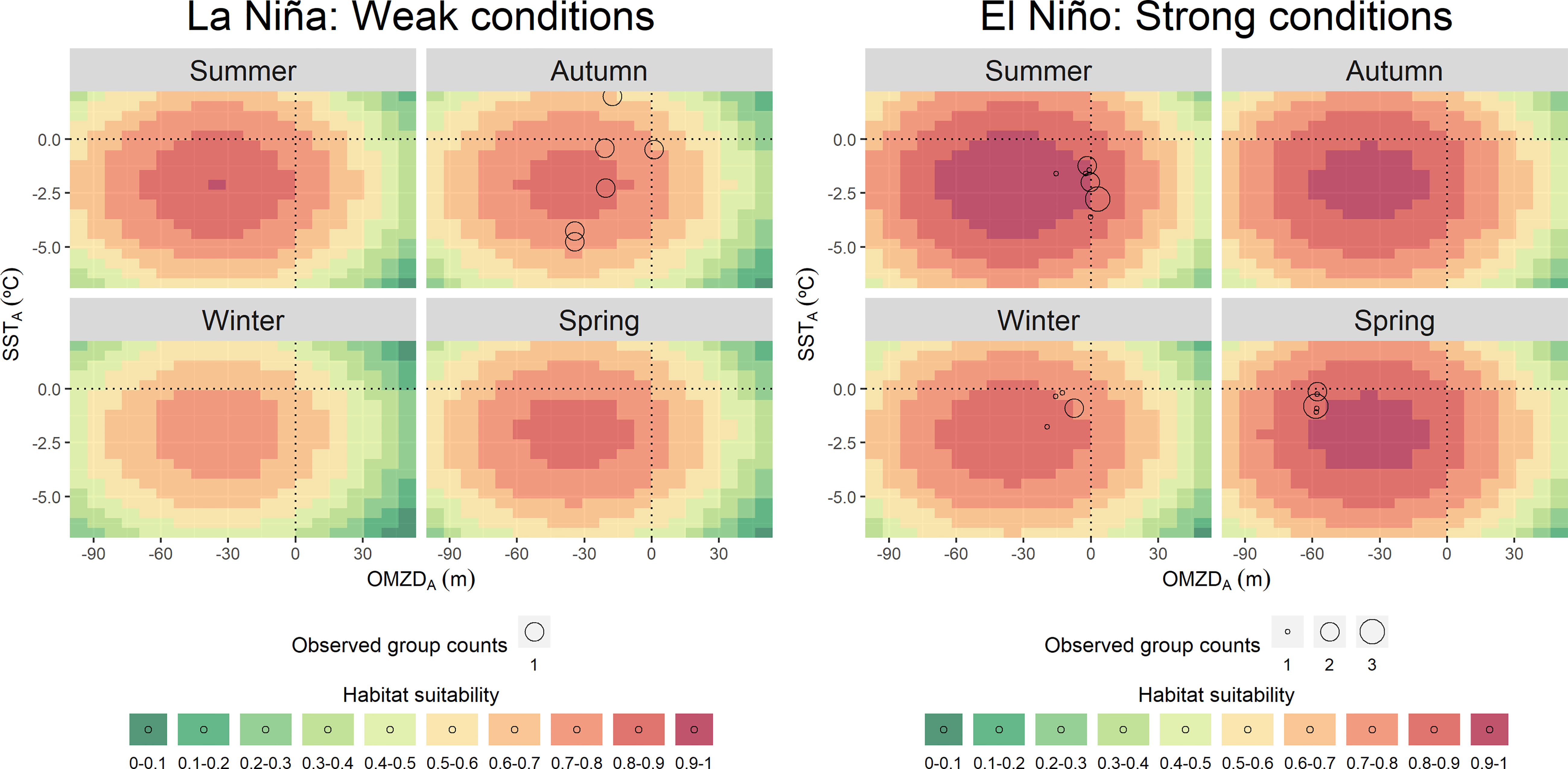
Figure 3 Predicted values of common dolphin (Delphinus delphis spp.) habitat suitability for a theoretical environmental space during La Niña and El Niño conditions, based on the covariates included in the best model: the oxygen minimum zone depth spatial anomaly (OMZD_A) and the remotely sensed chlorophyll-a concentration spatial anomaly (CHL_A). Empty circle size represents the observed group counts in each sample unit (i.e., transect).

Bottlenose dolphins showed preferences for both cold and warm waters in areas with shallow OMZ. Broad values of SST_A (-4 to 4 °C) and negative OMZ_A (0 to -80 m) predicted the highest habitat suitability (0.7 – 1) mainly in summer. During the rest of the seasons, the pattern persisted with lower habitat suitability values (up to 0.8) (Figure 1). The species aggregated mainly in oceanic waters along the entire Peruvian coast (Figure 2). However, two spots of high habitat suitability (0.7-1) were predicted between 6-11° and 14° S, during all seasons. During autumn, the species retracted to more oceanic waters in the central spot with higher habitat suitability off north central Peru, with median distances to the coast of 86.2 km (95%-CI: 82.3 – 90.4) (Supplementary Material, Appendix 6, Figures A.6.3). During summer, the potential distribution was broader in both oceanic and coastal areas (81.9 km; 95%-CI: 78.3 – 85.5; Supplementary Material, Appendix 6, Figures A.6.3), mainly in the north-central (7 - 11° S) region, where the largest groups were observed in transitional waters on the continental shelf-edge. During winter and spring, the species retracted partially to coastal waters in the central spot with higher habitat suitability off north central Peru, 76.3 km (95%-CI: 72 – 80.5) and 71.8 km (95%-CI: 67 – 76.7), respectively (Supplementary Material, Appendix 6, Figures A.6.3). The coastal area between 14-17°S also presented low habitat suitability values (0 - 0.4) for bottlenose dolphins, like those of common dolphins. Although the species’ habitat suitability did not present strong seasonal effects, the northern spot (7 - 11° S) showed the highest values during summer (Figure 2). Higher values were predicted during El Niño (up to 1) compared to those during La Niña (up to 0.9) (Figures 4, 6). The best habitats concentrated mainly at 7 - 11° S and ~14° S, and were broader during El Niño strong conditions, especially in summer (Figure 6).

FIGURE 4

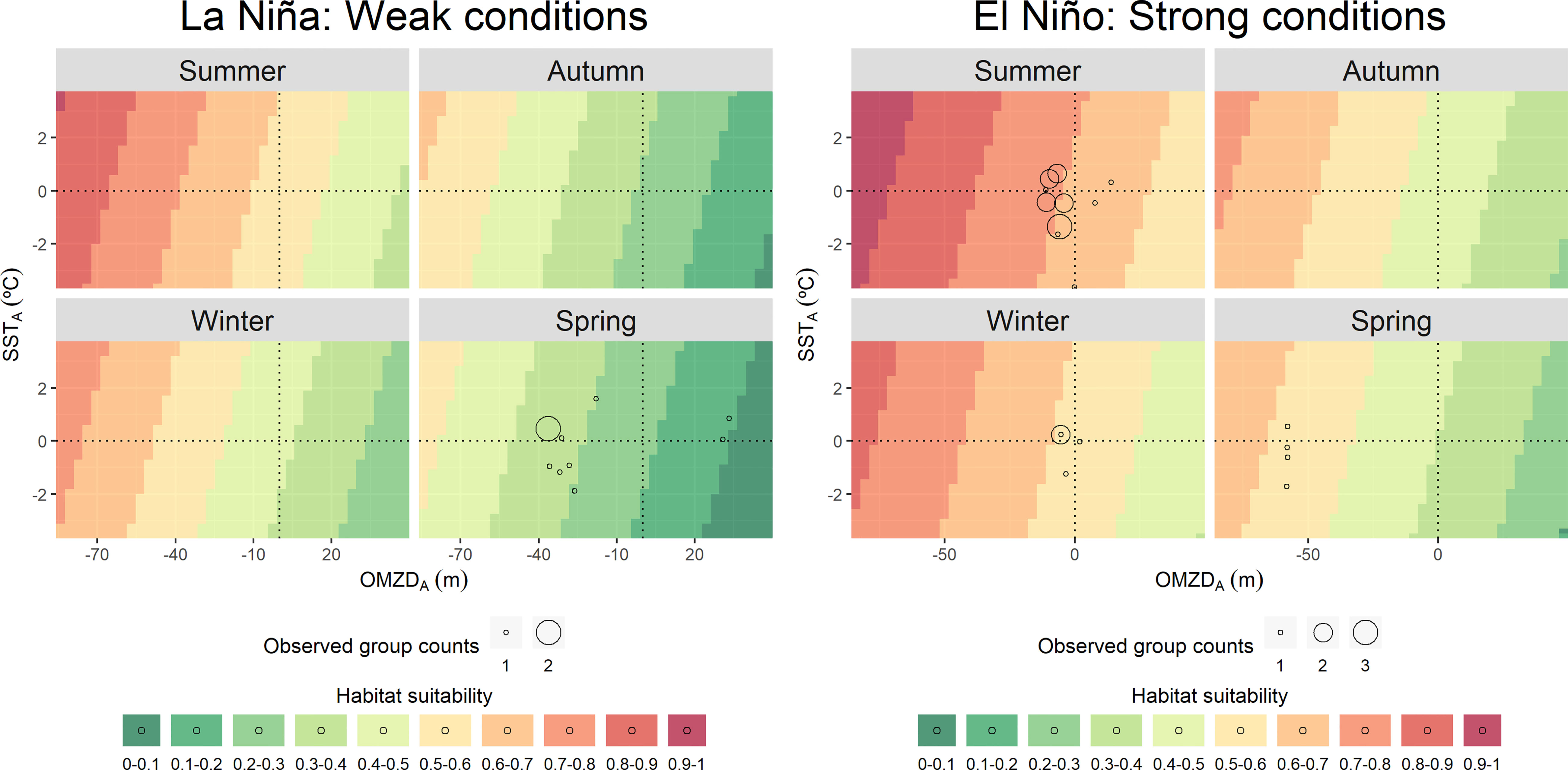
Figure 4 Predicted values of bottlenose dolphin (Tursiops truncatus) habitat suitability for a theoretical environmental space during La Niña and El Niño conditions, based on the covariates included in the best model: the oxygen minimum zone depth spatial anomaly (OMZD_A) and the remotely sensed chlorophyll-a concentration spatial anomaly (CHL_A). Empty circle sizes represent the observed group counts in each sample unit (i.e., transect).

FIGURE 5

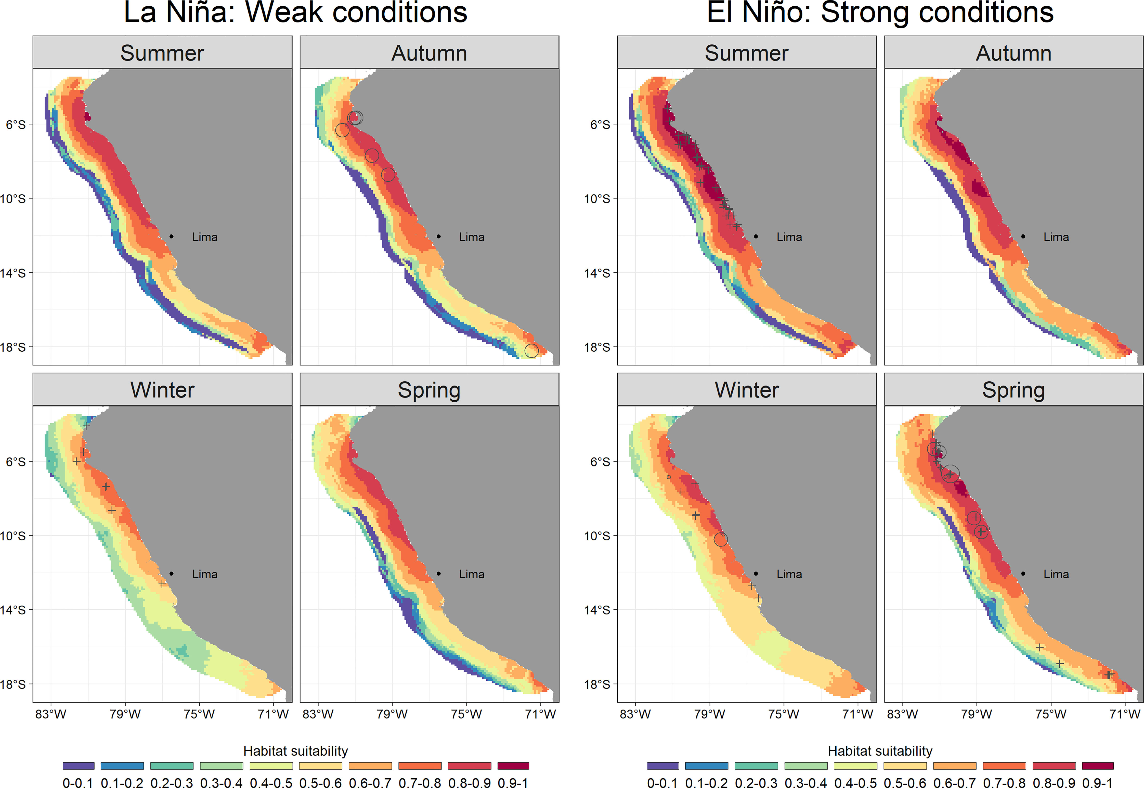
Figure 5 Predicted values of common dolphin (Delphinus delphis spp.) habitat suitability for the geographical space during La Niña and El Niño conditions. Empty circle sizes represent the observed group counts in each sample unit (i.e., transect). Crosses represent validation data, not included as data in the model.

FIGURE 6

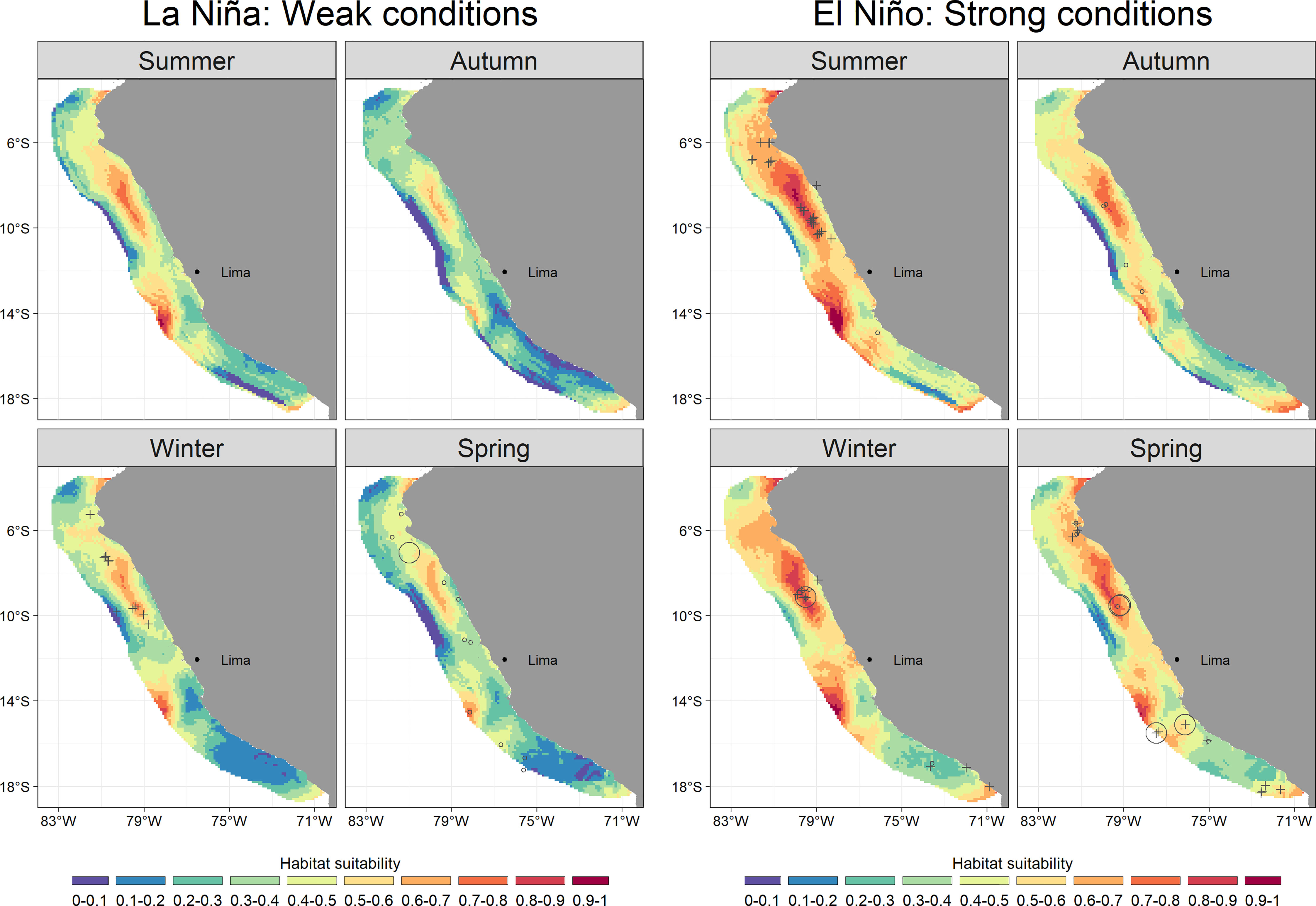
Figure 6 Predicted values of bottlenose dolphin (Tursiops truncatus) habitat suitability for the geographical space during La Niña and El Niño conditions. Empty circle size represents the observed group counts in each sample unit (i.e., transect). Crosses represent validation data, not included as data in the model.

It is important to point out that model predictions for the austral winter were less represented by data than those from the rest of the seasons, both for cetacean observations and for OMZD and DP casts. Nevertheless, the effect of this weakness of sample size on the prediction was quantified in terms of uncertainty. Indeed, the winter predictions showed higher values of posterior standard deviations for all three species (Figures A7.1–A7.3).

4. Discussion

This is the first study estimating the importance of the OMZ depth for cetacean distributions. Our results showed dusky and common dolphins occupy cold productive waters with shallow OMZ. This suggests both species would exploit areas where their main prey, the Peruvian anchovy, is constrained and thus more accessible. Bottlenose dolphins depicted a different pattern. Although their distribution was related to relative shallow OMZ areas, their habitat preferences were wider in terms of water temperature, suggesting plasticity for more diverse prey and the use of different foraging strategies.

Models predicted an extended westward distribution of both dusky and common dolphins mainly during austral summer and autumn, and a contraction to the coast in winter. During summer, weak upwelling maintains cold water masses with high primary productivity only in coastal areas (Figure 7; Supplementary Material, Appendix 3, Figures A.3.2; A3.3), restricting the horizontal distribution of anchovy (Swartzman et al., 2008). During winter, an intense upwelling and the occurrence anticyclonic eddies (Chaigneau et al., 2008) promote a westward expansion of cold waters (Figure 7; Supplementary Material, Appendix 3, Figures A.3.2; A3.3) and consequently the horizontal distribution of anchovy (Swartzman et al., 2008). Initially, this could indicate a larger extension of foraging areas for predators, however, results showed a spatial contraction during this season. This apparent contradiction could result from the seasonal variation in OMZ depth, because it modulates prey accessibility. During summer, OMZ is shallow (ca. 20 m; Graco et al., 2017) over the continental shelf (negative spatial anomalies: Supplementary Material, Appendix 3, Figure A.3.1), constraining the vertical distribution of anchovy (Passuni et al., 2016) and the consequent expansion of easily catchable prey for dusky and common dolphins. Contrastingly, OMZ was relatively deeper (ca. 60 m; Graco et al., 2017) in winter over the continental shelf (positive spatial anomalies: Supplementary Material, Appendix 3, Figure A.3.1), allowing for the anchovy’s vertical dispersion (Passuni et al., 2016). Only a narrow coastal strip maintained a shallow OMZ where prey would be still easily catchable to dusky and common dolphins (Supplementary Material, Appendix 3, Figure A.3.1).

FIGURE 7

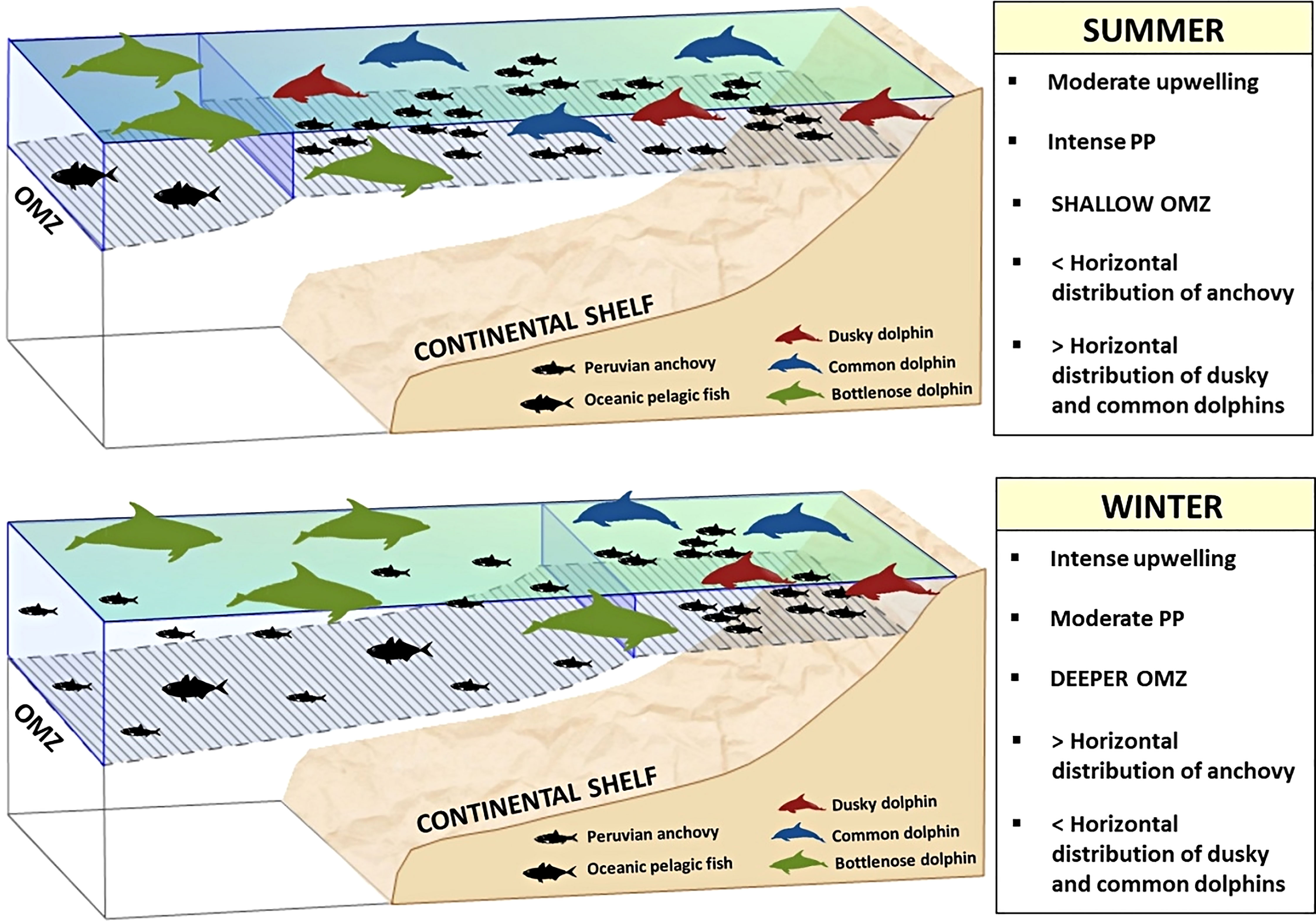
Figure 7 Conceptual model of habitat suitability of dusky, common, and bottlenose dolphins in the northern Humboldt Current System. Two contrasting seasons (summer and winter) are shown to represent differences in the species spatial distribution, mainly over the continental shelf. PP: Primary productivity. Dolphin shapes were modified from those of Chris Huh (https://creativecommons.org/licenses/by-sa/3.0/).

The persistent affinity of these two species to areas with shallow OMZ regardless of the season could respond to their higher metabolic costs of living (Mckinnon, 1994; Spitz et al., 2012), the large pods of hundreds to thousands of individuals they conform, and their very active behavior. Such high demands would imply these two species must maximize the energy intake by foraging on intense productivity areas around upwelling cores (Jefferson et al., 2009; Manocci et al., 2014; Llapapasca et al., 2018), and consume abundant prey (Sih and Christensen, 2001) of higher caloric density, such as clupeids (Spitz et al., 2010; Spitz et al., 2012), and anchovies (6.5 Kj g^-1; Mckinnon, 1994). However, the fact that the best habitat suitability models for these two species included always shallow OMZ relative depths as key driver during all seasons, suggests they also select areas of high prey accessibility to maximize energy intake. Therefore, the limited vertical distribution of anchovies by a shallow OMZ could confer an important advantage to these predators, arguably improving foraging success. This relation was slightly weaker in common dolphins than in dusky dolphins, probably because the former also distributes in northern Peru (3 - 6° S), where there is a strong influence of the southern branch of the Cromwell subsurface current of more oxygenated waters (> 1 ml l^-1) (Zuta and Guillén, 1970), and therefore the OMZ deepens to ~100 m (Graco et al., 2007).

A shallow pycnocline or thermocline could also aggregate prey for predators since it triggers productive cores, as observed in the eastern tropical Pacific (Reilly, 1990; Scott et al., 2012). Nevertheless, this variable was less relevant in our models likely due its strong seasonal pattern. It is developed during summer, up to 50–60-m depth off north Peru, but virtually absent during winter (Zuta and Guillén, 1970). Also, a shallow thermocline assures nutrient rich waters occupy the euphotic zone, triggering high primary production and prey aggregation, but it does not limit prey physiologically as the OMZ does. However, this interpretation must be taken with caution due to the least amount of data to this variable in our study.

In general, a more oceanic distribution was predicted for bottlenose dolphins, in areas of persistently shallow OMZ with both cold and warm waters. In general, the species showed a more oceanic distribution pattern which would allow them to exploit a niche not occupied by dusky or common dolphins. The potential habitat of the species displaced to more coastal areas in winter and spring when the distribution of dusky and common dolphins was also more restricted towards the coast. Bottlenose dolphin’s diet is more diverse, consuming epipelagic and mesopelagic species (Jefferson et al., 2008). In Peruvian waters, the species also feeds mainly on mackerels, myctophids, and barracudas, as well as lower quantities of anchovies (García-Godos et al., 2007). The energy supply of its dominant prey is lower than that of anchovies (6.5 kJ g^-1). Myctophids contain 4.1 kJ g^-1 and mackerels 5.4 kJ g^-1 (Mckinnon, 1994; Spitz et al., 2010). The lower energetic requirements of bottlenose dolphins, compared to those of common dolphins, have been confirmed by their lower mitochondrial density in muscles (Spitz et al., 2012). Their prey could react differently to the OMZ depth. Jack mackerels rest in the upper limit of the OMZ reducing its activity (Bertrand et al., 2006). Likewise, it is known that mesopelagic species such as myctophids remain lethargic under very low oxygen concentrations (Jones, 1971; Kramer, 1987), as a strategy for avoiding epipelagic predators not adapted for hypoxic conditions (Barham, 1970). This prey behavior is arguably exploited by cetaceans adapted for deeper diving such as bottlenose dolphins, which could easily catch immobile prey. Such strategy would compensate for the lower prey quality in terms of energy.

Our results showed spatial segregation among species, suggesting habitat partitioning of the NHCS. Dusky and common dolphins showed preference for the continental shelf, although separated latitudinally. Bottlenose dolphins preferred the shelf-break and oceanic waters. Habitat and niche partitioning occur as response to the resource competition (Bearzi, 2005; Oviedo et al., 2018). Indeed, dusky and common dolphins shared the environmental space related to cold-productive waters with shallow OMZ, therefore latitudinal differences would allow reduce partially the inter-specific competition. In the same way, the occupation of oceanic waters by bottlenose dolphin allows the exploitation of a different niche not occupied by coastal dolphins. Models also showed a seasonal effect on the habitat suitability of the three dolphin species, which could be related to different factors. The spatial distribution of the predictors varying seasonally could have been captured, but also potential seasonality in the species’ life history, not necessarily linked to the predictors, such as their reproductive cycles. Dusky dolphins exhibit a highly seasonal reproductive cycle in Peruvian waters, with a peak breeding season during the austral winter and a calving season during late winter-early spring (Van Waerebeek and Read, 1994), when high habitat suitability predictions restrict more to the coast. Although there is no information about a seasonal reproductive cycle for common dolphins in the HCS, it cannot be discarded. The southern ETP’s population of short-beaked common dolphins (Delphinus delphis delphis) has a well-defined breeding period from January to July (Perryman and Lynn, 1993) while the central ETP’s population exhibits it throughout the year (Perryman and Lynn, 1993; Danil and Chivers, 2007). It seems this difference is due to the strong productivity pulses in temperate waters compared to those of more tropical waters. Bottlenose dolphin habitat suitability was also affected by the seasonal signal; however, its reproductive cycle is unknown for the study area and adjacent zones.

Interannual effects improved common and bottlenose dolphins habitat suitability models but not that of dusky dolphins. This could be due to the ICEN’s spatial coverage, which encompasses mainly the northern-central Peru (3-10° S), less occupied by dusky dolphins. The main interannual effect was an increase of habitat suitability in the main aggregation spots of common and bottlenose dolphins during ‘El Niño strong condition’ indicating a major aggregation of dolphins in these areas that arguably remained relatively productive and therefore would exhibit highest habitat suitability values. These warm anomalies also deepen the OMZ (> 100 m) off northern-central Peru in coastal areas (Graco et al., 2007) allowing the anchovy to disperse vertically (Gutiérrez, 2001), which would force common dolphins to forage in deeper waters. The increase in high habitat suitability coverage for bottlenose dolphins could respond to the incursion of more oceanic prey, which follow the eastward intrusion of warm oceanic waters (Ñiquen and Bouchon, 2004). No evident latitudinal changes were detected in warm conditions, coinciding with the reports for 1997-98 El Niño, during which coastal upwelling cells remained active, exporting primary production offshore, and providing refuge areas to anchovies, mackerels, other pelagic fish (Bertrand et al., 2004), and delphinids (Llapapasca et al., 2018). Contrastingly, ‘La Niña weak conditions’ produced very similar habitat suitability predictions to those of ‘neutral conditions’, suggesting a weak or null impact on the distributions of both species during weak anomalies.

Our findings suggest the OMZ relative depth in space plays a relevant role in the distribution of the dominant dolphin species of the NHCS, potentially modulating the accessibility to their main prey, the Peruvian anchovy. In fact, areas with relatively shallow OMZ were selected during all seasons, mainly by dusky and common dolphins. These two species would maximize their energy gain by consuming highly caloric prey, restricted vertically to the upper oxygenated layers. Bottlenose dolphins showed affinity for more oceanic and warmer waters, where they could exploit more mesopelagic prey.

Some predictions of climate change for the next 78 years in the NHCS include intense surface warming (2 - 4.5 °C) of waters on the oceanic shelves and lower values of dissolved oxygen concentrations could be expected (Echevin et al., 2020). Such future conditions would be similar to those of the last interglacial period (130 to 116 thousand years ago), when the fish community was dominated by goby and mesopelagic fishes instead anchovies (Salvatteci et al., 2022). For the latter, these conditions are detrimental, especially for recruitment, in spite of the species broad thermal tolerance (Echevin et al., 2020). This in turn, can trigger the species poleward migration toward cooler waters (Cheung et al., 2018). According to our results, these could mean a long-term effect on the habitat quality and distribution of dolphins in the NHCS.

Data availability statement

Oxygen concentrations from 2001 to 2005 are freely available at http://wod.iode.org/SELECT/dbsearch/dbsearch.html. Oxygen concentrations for 2007-2019, as well as cetacean data, may be requested at https://www.gob.pe/imarpe.

Ethics statement

Ethical review and approval was not required for the animal study because This study did not involve any animal handling or any direct contact with the animals. The data are purely observational.

Author contributions

Conception and experiment design: ML and MP. Data processing: ML, MP and DG. Data analysis: ML and MP. Model design and construction: ML and MP. Interpretation of results: ML, MP, DG, and JQ. Writing-original draft: ML. Review and editing: MP, ML, DG, and JQ. Figure production: ML. All authors contributed to the article and approved the submitted version.

Funding

Oceanographic and biological data were acquired by IMARPE’s with its own public funds. A full PhD scholarship was granted by Consejo Nacional de Ciencia y Tecnología (CONACYT) to M. Llapapasca. M.A. Pardo was funded by CICESE (Internal Project No. 691–113) during the preparation of this manuscript.

Acknowledgments

M. Llapapasca is grateful to Oficina de Investigaciones en Depredadores Superiores and Dirección de Investigaciones Oceanográficas y Cambio Climático at IMARPE for granting access to cetacean and oceanographic data, as well as to the Marine Macroecology Laboratory at CICESE – Unidad La Paz, for the research internship during the preparation of this study. Thanks to A. Pacheco for his valuable comments on an early version, and to the reviewers who helped us to improve this manuscript.

Conflict of interest

The authors declare that the research was conducted in the absence of any commercial or financial relationships that could be construed as a potential conflict of interest.

Publisher’s note

All claims expressed in this article are solely those of the authors and do not necessarily represent those of their affiliated organizations, or those of the publisher, the editors and the reviewers. Any product that may be evaluated in this article, or claim that may be made by its manufacturer, is not guaranteed or endorsed by the publisher.

Supplementary material

The Supplementary Material for this article can be found online at: https://www.frontiersin.org/articles/10.3389/fmars.2022.1027366/full#supplementary-material

References

Ballance L. T., Pitman R. L., Fiedler P. C. (2006). Oceanographic influences on seabirds and cetaceans of the eastern tropical pacific: a review. Prog. Oceanogr. 69 (2–4), 360–390. doi: 10.1016/j.pocean.2006.03.013

CrossRef Full Text | Google Scholar

Ballance L. T., Pitman R. L., Reilly S. B. (1997). Seabird community structure along a productivity gradient: importance of competition and energetic constraint. Ecology 78, 1502–1518. doi: 10.1890/0012-9658(1997)078[1502:SCSAAP]2.0.CO;2

CrossRef Full Text | Google Scholar

Barbraud C., Bertrand A., Bouchón M., Chaigneau A., Delord K., Demarcq H., et al. (2018). Density dependence, prey accessibility and prey depletion by fisheries drive Peruvian seabird population dynamics. Ecography 41 (7), 1092–1102. doi: 10.1111/ecog.02485

CrossRef Full Text | Google Scholar

Barham E. G. (1970). “Deep sea fishes: lethargy and vertical orientation,” in Biological sound scattering in the ocean, report 005. Ed. Farquahar G. B. (Maury Center for Ocean Science, Washington, DC: US Government Printing Office), 100–118.

Google Scholar

Barlow J., Kahru M., Mitchell B. G. (2008). Cetacean biomass, prey consumption, and primary production requirements in the California current ecosystem. Mar. Ecol. Prog. Ser. 371, 285–295. doi: 10.3354/meps07695

CrossRef Full Text | Google Scholar

Bearzi M. (2005). Dolphin sympatric ecology. Mar. Biol. Res. 1 (3), 165–175. doi: 10.1080/17451000510019132

CrossRef Full Text | Google Scholar

Bertrand A., Barbieri M., Gerlotto F., Leiva and F., Córdova J. (2006). Determinism and plasticity of fish schooling behavior as exemplified by the south pacific jack mackerel trachurus murphyi. Mar. Ecol. Prog. Ser. 311, 145–156. doi: 10.3354/meps311145

CrossRef Full Text | Google Scholar

Bertrand A., Chaigneau A., Peraltilla S., Ledesma J., Graco M., Monetti F., et al. (2011). Oxygen: a fundamental property regulating pelagic ecosystem structure in the coastal southeastern tropical pacific. PloS One 6, (12). doi: 10.1371/journal.pone.0029558

CrossRef Full Text | Google Scholar

Bertrand A., Gerlotto F., Bertrand S., Gutierrez M., Alza L., Chipollini A., et al. (2008). Schooling behavior and environmental forcing in relation to anchoveta distribution: An analysis across multiple spatial scales. Prog. Oceanogr. 79, 264–277. doi: 10.1016/j.pocean.2008.10.018

CrossRef Full Text | Google Scholar

Bertrand A., Grados D., Colas F., Bertrand S., Capet X., Chaigneau A., et al. (2014). Broad impacts of fine-scale dynamics on seascape structure from zooplankton to seabirds. Nat. Commun. 5, 5239. doi: 10.1038/ncomms6239

PubMed Abstract | CrossRef Full Text | Google Scholar

Bertrand A., Segura M., Gutiérrez M., Vásquez L. (2004). From small-scale habitat loopholes to decadal cycles: a habitat-based hypothesis explaining fluctuation in pelagic fish populations off Peru. Fish Fisheries. 5, 296–316. doi: 10.1111/j.1467-2679.2004.00165.x

CrossRef Full Text | Google Scholar

Boyd C., Castillo R., Hunt G. L. Jr, Punt A. E., VanBlaricom G. R., Weimerskirch H., et al. (2015). Predictive modelling of habitat selection by marine predators with respect to the abundance and depth distribution of pelagic prey. J. Anim. Ecol. 84, 1575–1588. doi: 10.1111/1365-2656.12409

PubMed Abstract | CrossRef Full Text | Google Scholar

Cañadas A., Sagarminaga R., García-Tiscar S. (2002). Cetacean distribution related with depth and slope in the Mediterranean waters off southern Spain. Deep Sea Res. I 49 (11), 2053–2073. doi: 10.1016/S0967-0637(02)00123-1

CrossRef Full Text | Google Scholar

Chaigneau A., Gizolme A., Grados C. (2008). Mesoscale eddies off Peru in altimeter records: Identification algorithms and eddy spatio-temporal patterns. Prog. Oceanogr. 79 (2–4), 106. doi: 10.1016/j.pocean.2008.10.013

CrossRef Full Text | Google Scholar

Cheung W. W. L., Bruggeman J., Butenschön J. (2018). “Projected changes in global and national potential marine fisheries catch under climate change scenarios in the twenty-first century,” in Impacts of climate change on fisheries and aquaculture: Synthesis of current knowledge, adaptation and mitigation options (Rome: Food and Agriculture Organization of United Nation), 628. Available at: http://www.fao.org/3/I9705EN/i9705en.pdf.

Google Scholar

Danil K., Chivers S. J. (2007). Growth and reproduction of female short-beaked common dolphins, delphinus delphis, in the eastern tropical pacific. Can. J. Zool. 85, 1. doi: 10.1139/z06-188

CrossRef Full Text | Google Scholar

Echevin V., Colas F., Espinoza-Morriberon D., Vasquez L., Anculle T., Gutierrez D. (2018). Forcings and evolution of the 2017 coastal El niño off northern Peru and Ecuador. Front. Mar. Sci. 5. doi: 10.3389/fmars.2018.00367

CrossRef Full Text | Google Scholar

Echevin V., Gévaudan M., Espinoza-Morriberon D., Tam J., Aumont O., Gutierrez D., et al. (2020). Physical and biogeochemical impacts of RCP8.5 scenario in the Peru upwelling system. Biogeosciences 17, 3317–3341. doi: 10.5194/bg-17-3317-2020

CrossRef Full Text | Google Scholar

Ekau W., Auel H., Pörtner H. O., Gilbert D. (2010). Impacts of hypoxia on the structure and processes in pelagic communities (zooplankton, macro-invertebrates and fish). Biogeosciences 7, 1669–1699. doi: 10.5194/bg-7-1669-2010

CrossRef Full Text | Google Scholar

Espinoza-Morriberón D., Echevin V., Colas F., Tam J., Gutierrez D., Graco M., et al. (2019). Oxygen Variability during ENSO in the Tropical South Eastern Pacific. Frontiers in Marine Science. 5, 526. doi: 10.3389/fmars.2018.00526

CrossRef Full Text | Google Scholar

Forney K. A., Ferguson M. C., Becker E. A., Fiedler P. C., Redfern J. V., Barlow J., et al. (2012). Habitat-based spatial models of cetacean density in the eastern pacific ocean. Endangered Spec. Res. 16, 113–133. doi: 10.3354/esr00393

CrossRef Full Text | Google Scholar

Fuenzalida R., Schneider W., Garcés-Vargas J., Bravo L., Lange C. (2009). Vertical and horizontal extension of the oxygen minimum zone in the eastern south pacific ocean. Deep Sea Res. Part II 56, 1027–1038. doi: 10.1016/j.dsr2.2008.11.001

CrossRef Full Text | Google Scholar

García-Godos I., Van Waerebeek K., Reyes J., Alfaro-Shigueto J., Arias-Schreiber M. (2007). Prey occurrence in the stomach contents of four small cetacean species in Peru. Latin Am. J. Aquat. Mammals 6 (2), 171–183. doi: 10.5597/lajam00122

CrossRef Full Text | Google Scholar

Garcia H. E., Locarnini R. A., Boyer T. P., Antonov J. I., Mishonov A. V., Baranova O. K., et al. (2010). World ocean atlas 2009, volume 3: Dissolved oxygen, apparent oxygen utilization, and oxygen saturation (Washington, D.C: U.S. Government Printing Office). NOAA Atlas NESDIS 70.

Google Scholar

Graco M., Ledesma J., Flores G., Girón M. (2007). Nutrientes, oxígeno y procesos biogeoquímicos en el sistema de surgencias de la corriente de Humboldt frente a perú. Rev. Peruana Biología 14, 117–128. doi: 10.15381/rpb.v14i1.2165

CrossRef Full Text | Google Scholar

Graco M. I., Purca S., Dewitte B., Castro C. G., Morón O., Ledesma J., et al. (2017). The OMZ and nutrient features as a signature of interannual and low-frequency variability in the Peruvian upwelling system. Biogeosciences 14 (20), 4601–4617. doi: 10.5194/bg-14-4601-2017

CrossRef Full Text | Google Scholar

Gutiérrez M. (2001). “Efectos del evento El niño 1997–98 sobre la distribución y abundancia de anchoveta (Engraulis ringens),” in El Niño en américa latina: impactos biológicos y sociales. Eds. Tarazona J., Arnts W. E., Castillo de Maruenda E. (Lima, Peru: Consejo Nacional de Ciencia y Tecnología), 55–72.

Google Scholar

Gutiérrez D., Akester M., Naranjo L. (2016). Productivity and sustainable management of the Humboldt current Large marine ecosystem under climate change. Environ. Dev. 17, 126–144. doi: 10.1016/j.envdev.2015.11.004

CrossRef Full Text | Google Scholar

Gutiérrez D., Enríquez E., Purca S., Quipúzcoa L., Marquina R., Flores G., et al. (2008). Oxygenation episodes on the continental shelf of central Peru: Remote forcing and benthic ecosystem response. Prog. Oceanogr. 79 (2-4), 177–189. doi: 10.1016/j.pocean.2008.10.025

CrossRef Full Text | Google Scholar

Ibanez-Erquiaga B., Pacheco A. S., Rivadeneira M. M., Tejada C. L. (2018). Biogeographical zonation of rocky intertidal communities along the coast of Peru (3.5 13.5° s southeast pacific). PloS One 13 (11), e0208244. doi: 10.1371/journal.pone.0208244

PubMed Abstract | CrossRef Full Text | Google Scholar

Jefferson T. A., Fertl D., Bolaños-Jiménez J., Zerbini A. (2009). Distribution of common dolphins (Delphinus spp.) in the western Atlantic ocean, a critical re-examination. Mar. Biol. 156, 1109–1124. doi: 10.1007/s00227-009-1152-y

CrossRef Full Text | Google Scholar

Jefferson T. A., Webber M. A., Pitman R. L. (2008). Marine mammals of the world, comprehensive guide to their identification (Elsevier, San Diego: Academic Press).

Google Scholar

Jones D. R. (1971). The effect of hypoxia and anaemia on the swimming performance of rainbow trout (Salmo gairdneri). J. Exp. Biol. 55, 541–551. doi: 10.1242/jeb.55.2.541

PubMed Abstract | CrossRef Full Text | Google Scholar

Kelley, Richards, WG127 SCOR/IAPSO (2017) Gsw: Gibbs Sea water functions. r package version 1.0-5. Available at: https://CRAN.R-project.org/package=gsw.

Google Scholar

Kokubun N., Takahashi A., Ito M., Matsumoto K., Kitaysky A., Watanuki Y. (2010). Annual variation in the foraging behavior of thick-billed murres in relation to upper-ocean thermal structure around st. George island, Bering Sea. Aquat. Biol. 8, 289–298. doi: 10.3354/ab00243

CrossRef Full Text | Google Scholar

Kramer D. L. (1987). Dissolved oxygen and fish behavior. Environ. Biol. Fishes 18, 81–92. doi: 10.1007/BF00002597

CrossRef Full Text | Google Scholar

Limburg K. E., Breitburg D., Swaney D. P., Jacinto G. (2020). Ocean deoxygenation: A primer. One Earth 2 (1), 24–29. doi: 10.1016/j.oneear.2020.01.001

CrossRef Full Text | Google Scholar

Llapapasca M. A., Pacheco A. S., Fiedler P., Goya E., Ledesma J., Peña C., et al. (2018). Modeling the potential habitats of dusky, commons, and bottle-nose dolphins in the Humboldt current system off Peru: The influence of non-El niño vs. El niño 1997-98 conditions and potential prey availability. Prog. Oceanogr. 168, 169–181. doi: 10.1016/j.pocean.2018.09.003

CrossRef Full Text | Google Scholar

Manocci L., Laran S., Monestiez P., Dorémus G., Van Canneyt O., Watremez P and Ridoux V. (2014). Predicting top predators habitats in the southwest Indian ocean. Ecography 37, 261–278. doi: 10.1111/j.1600-0587.2013.00317.x

CrossRef Full Text | Google Scholar

Mckinnon J. (1994). Feeding habits of the dusky dolphin lagenorhynchus obscurus, in the coastal waters of central Peru. Fishery Bull. 92 (3), 569–578. Available at: https://spo.nmfs.noaa.gov/sites/default/files/pdf-content/1994/923/mckinnon.pdf.

Google Scholar

Meyer X., MacIntosh A. J. J., Chiaradia A., Kato A., Ramírez F., Sueur C., et al. (2020). Oceanic thermal structure mediates dive sequences in a foraging seabird. Ecol. Evol. 10 (13), 6610–6622. doi: 10.1002/ece3.6393

PubMed Abstract | CrossRef Full Text | Google Scholar

Mogollón R., Calil P. H. R. (2017). On the effects of ENSO on ocean biogeochemistry in the northern Humboldt current system (NHCS): A modeling study. J. Mar. Syst. 172, 137–159. doi: 10.1016/j.jmarsys.2017.03.011

CrossRef Full Text | Google Scholar

Naimi B., Hamm N. A. S., Groen T. A., Skidmore A. K., Toxopeus A. G. (2014). Where is positional uncertainty a problem for species distribution modelling? Ecography 37 (2), 191–203. doi: 10.1111/j.1600-0587.2013.00205.x

CrossRef Full Text | Google Scholar

Ñiquen M., Bouchon M. (2004). Impact of El niño events on pelagic fisheries in Peruvian waters. Deep Sea Res. II 51, 563–574. doi: 10.1016/j.dsr2.2004.03.001

CrossRef Full Text | Google Scholar

Oschlies A., Brandt P., Stramma L., Schmidtko S. (2018). Drivers and mechanisms of ocean deoxygenation. Nat. Geosci. 11 (7), 467–473. doi: 10.1038/s41561-018-0152-2

CrossRef Full Text | Google Scholar

Oviedo L., Fernández M., Herra-Miranda B., Pacheco-Polanco J. D., Hernández-Camacho C., Aurioles-Gamboa D. (2018). Habitat partitioning mediatesthe coexistence of sympatric dolphins in a tropicalfjord-like embayment. J. Mammal. 99 (3), 554–564. doi: 10.1890/14-1134.1

CrossRef Full Text | Google Scholar

Passuni G., Barbraud C., Chaigneau A., Demarcq H., Ledesma J., Bertrand A., et al. (2016). Seasonality in marine ecosystems: Peruvian seabirds, anchovy, and oceanographic conditions. Ecology 97 (1), 182–193. doi: 10.1890/14-1134.1

PubMed Abstract | CrossRef Full Text | Google Scholar

Perrin W. F. (2018). Common Dolphin: Delphinus delphis, Editor(s): Würsig B., Thewissen J. G. M., Kovacs K. M., Encyclopedia of Marine Mammals (Third Edition) (Academic Press) 205–209. doi: 10.1016/B978-0-12-804327-1.00095-9

CrossRef Full Text | Google Scholar

Perryman W. L., Lynn M. S. (1993). Identification of geographic forms of common dolphin (Delphinus delphis) from aerial photogrammetry. Mar. Mammal Sci. 9 (2), 119–137. doi: 10.1111/j.1748-7692.1993.tb00438.x

CrossRef Full Text | Google Scholar

Peterson B. G., Carl P. (2020) PerformanceAnalytics: Econometric tools for performance and risk analysis. Available at: https://CRAN.R-project.org/package=PerformanceAnalytics.

Google Scholar

Plummer M. (2003). “JAGS: A program for analysis of Bayesian graphical models using Gibbs sampling,” in Proceedings of the 3rd international workshop on distributed statistical computing (Hornik K., Leisch F., Zeileis A. (eds)) 1–10. Available at: https://www.r-project.org/conferences/DSC-2003/.

Google Scholar

Prince E. D., Goodyear C. P. (2006). Hypoxia-based habitat compression of tropical pelagic fishes. Fisheries Oceanogr. 15, 451–464. doi: 10.1111/j.1365-2419.2005.00393.x

CrossRef Full Text | Google Scholar

Proud R., Le Guen C., Sherley R. B., Kato A., Ropert-Coudert Y., Ratcliffe N., et al. (2021). Using Predicted Patterns of 3D Prey Distribution to Map King Penguin Foraging Habitat. Frontiers in Marine Science. 8, 745200. doi: 10.3389/fmars.2021.745200

CrossRef Full Text | Google Scholar

R Core Team (2021). R: A language and environment for statistical computing (Vienna, Austria: R Foundation for Statistical Computing). Available at: https://www.R-project.org/.

Google Scholar

Redfern J. V., Ferguson M. C., Becker E. A., Hyrenbach K. D., Barlow J., Kaschner K., et al. (2006). Techniques for cetacean–habitat modeling: a review. Mar. Ecol. Prog. Ser. 310, 271–295. doi: 10.3354/meps310271

CrossRef Full Text | Google Scholar

Reilly S. B. (1990). Seasonal changes in distribution and habitat differences among dolphins in the eastern tropical pacific. Mar. Ecol. Prog. Ser. 66, 1–11. doi: 10.3354/meps066001

CrossRef Full Text | Google Scholar

Roberts J. J., Best B. D., Mannocci L., Fujioka E., Halpin P. N., Palka D. L., et al. (2016). Habitat-based cetacean density models for the U.S. Atlantic and gulf of Mexico. Sci. Rep. 6, 22615.

PubMed Abstract | Google Scholar

Ropert-Coudert Y., Kato A., Chiaradia A. (2009). Impact of small-scale environmental perturbations on local marine food resources: a case study of a predator, the little penguin. Proc. R. Soc. B: Biol. Sci. 276 (1676), 4105–4109. doi: 10.1098/rspb.2009.1399

CrossRef Full Text | Google Scholar

Rue H., Martino S., Chopin N. (2009). Approximate Bayesian inference for latent Gaussian models by using integrated nested Laplace approximations. J. R. Stat. Society Ser. B 71, 319–392. doi: 10.1111/j.1467-9868.2008.00700.x

CrossRef Full Text | Google Scholar

Saha K., Zhao X., Zhang H.-m., Casey K. S., Zhang D., Baker-Yeboah S., et al. (2018). AVHRR pathfinder version 5.3 level 3 collated (L3C) global 4km sea surface temperature for 1981-present. NOAA national centers for environmental information. Dataset. doi: 10.7289/v52j68xx

CrossRef Full Text | Google Scholar

Salvatteci R., Schneider R. R., Galbraith E., Field D. B., Blanz T., Bauersachs T., et al. (2022). Smaller fish species in a warm and oxygen-poor Humboldt current system. Science 375, 101–104. doi: 10.1126/science.abj0270

PubMed Abstract | CrossRef Full Text | Google Scholar

Scott M. D., Chivers S. J., Olson R. J., Fiedler PC and Holland K. (2012). Pelagic predator associations: tuna and dolphins in the eastern tropical pacific ocean. Mar. Ecol. Prog. Ser. 458, 283–302. doi: 10.3354/meps09740

CrossRef Full Text | Google Scholar

Sih A., Christensen B. (2001). Optimal diet theory: when does it work, and when and why does it fail? Anim. Behav. 61, 379–390. doi: 10.1006/anbe.2000.1592

CrossRef Full Text | Google Scholar

Soto K. H., Trites A. W., Arias-Schreiber M. (2006). Changes in diet and maternal attendance of south American sea lions indicate changes in the marine environment and prey abundance. Mar. Ecol. Prog. Ser. 312, 277–290. doi: 10.3354/meps312277

CrossRef Full Text | Google Scholar

Spitz J., Mourocq E., Leauté J.-P., Quéro J-C. and Ridoux V. (2010). Prey selection by the common dolphin: Fulfilling high energy requirements with high quality food. J. Exp. Mar. Biol. Ecol. 390, 73–77. doi: 10.1016/j.jembe.2010.05.010

CrossRef Full Text | Google Scholar

Spitz J., Trites A. W., Becquet V., Brind'Amour. A., Cherel Y., et al. (2012). Cost of living dictates what whales, dolphins and porpoises eat: The importance of prey quality on predator foraging strategies. PloS One 7, e50096. doi: 10.1371/journal.pone.0050096

PubMed Abstract | CrossRef Full Text | Google Scholar

Stephens D. W. (2008). Decision ecology: Foraging and the ecology of animal decision making. Cognitive Affective Behav. Neurosci. 8 (4), 475–484. doi: 10.3758/cabn.8.4.475

CrossRef Full Text | Google Scholar

Stramma L., Prince E. D., Schmidtko S., Luo J., Hoolihan J. P., Visbeck M., et al. (2012). Expansion of oxygen minimum zones may reduce available habitat for tropical pelagic fishes. Nat. Climate Change 2, 33–37. doi: 10.1038/nclimate1304

CrossRef Full Text | Google Scholar

Swartzman G., Bertrand A., Gutiérrez M., Bertrand S., Vasquez L. (2008). The relationship of anchovy and sardine to water masses in the Peruvian Humboldt current system from 1983–2005. Prog. Oceanogr. 79, 228–237. doi: 10.1016/j.pocean.2008.10.021

CrossRef Full Text | Google Scholar

Takahashi K., Martínez A. G. (2017). The very strong coastal El niño in 1925 in the far-eastern pacific. Climate Dynamic. 52, 7389–7415. doi: 10.1007/s00382-017-3702-1

CrossRef Full Text | Google Scholar

Takahashi K., Mosquera K., Reupo J. (2014). El Índice costero El niño (ICEN): historia y actualización. Boletín técnico: Generación Modelos climáticos para el pronóstico la ocurrencia del Fenómeno El Niño 1 (2), 8–9. Available at: http://hdl.handle.net/20.500.12816/4639

Google Scholar

Thomsen S., Kanzow T., Colas F., Echevin V., Krahmann G., Engel A. (2016). Do submesoscale frontal processes ventilate the oxygen minimum zone off Peru? Geophysical Research Letters 43 (15), 8133–8142. doi: 10.1002/2016gl070548

CrossRef Full Text | Google Scholar

Van Waerebeek K., Read A. J. (1994). Reproduction of dusky dolphins lagenorhynchus obscurus from coastal Peru. J. Mammal. 75, 1054–1062. doi: 10.2307/1382489

CrossRef Full Text | Google Scholar

Van Waerebeek K., Reyes J. C., Read A. J., Mckinnon J. S. (1990). “Preliminary observations of bottlenose dolphins from the pacific coast of south America,” in The bottlenose dolphin. Eds. Leatherwood S., Reeves R. R. (San Diego: Academic Press), 143–154.

Google Scholar

Van Waerebeek K., Würsig B. (2018). Dusky Dolphin: Lagenorhynchus obscurus. Editor(s): Würsig B., Thewissen J. G. M., Kovacs K. M., Encyclopedia of Marine Mammals (Third Edition). (Academic Press) Pages 277–280. doi: 10.1016/B978-0-12-804327-1.00111-4

CrossRef Full Text | Google Scholar

Vaquer-Sunyer R., Duarte C. M. (2008). Thresholds of hypoxia for marine biodiversity. Proc. Natl. Acad. Sci. United States America 105, 15452–15457. doi: 10.1073/pnas.080383310

CrossRef Full Text | Google Scholar

Vergara O., Dewitte B., Montes I., Garçon V., Ramos M., Paulmier A., et al. (2016). Seasonal variability of the oxygen minimum zone off Peru in a high-resolution regional coupled model. Biogeosciences 13 (15), 4389–4410. doi: 10.5194/bg-13-4389-2016

CrossRef Full Text | Google Scholar

Wang C., Fiedler P. C. (2006). ENSO variability in the eastern tropical pacific: A review. Prog. Oceanogr. 69 (2–4), 239–266. doi: 10.1016/j.pocean.2006.03.004

CrossRef Full Text | Google Scholar

Zuta S., Guillén O. (1970). Oceanografía de las aguas costeras del perú. Bol. Inst. Mar. Perú 2 (5), 157–324. Available at: https://revistas.imarpe.gob.pe/index.php/boletin/article/view/249

Google Scholar

Zuur A. F., Ieno E. N., Saveliev A. A. (2017). Beginner's guide to spatial, temporal and spatial-temporal ecological data analysis with r-INLA (Highland Statistcs Ltd). Available at: https://www.highstat.com/index.php/beginner-s-guide-to-regression-models-with-spatial-and-temporal-correlation.

Google Scholar