Variational parameter estimation in a two-equation turbulence model: A case study with a 3D primitive-equation ocean model

A three-dimensional and complete adjoint model of the Princeton Ocean Model with a generalized coordinate system (POMgcs) is developed to construct the 4D-Variational data assimilation (4D-Var) algorithm in this study. Uncertain parameters in the Mellor-Yamada 2.5 turbulence submodel (MY-2.5) which is enclosed in POMgcs, are tentatively estimated via the 4D-VAR algorithm within a biased model framework. Here, the control variables in the biased model are set to two uncertain wave-affected parameters (wave energy factor α and Charnock coefficient β ) in the MY-2.5 turbulence model, which play a crucial role in modulating the heat content distribution in the upper coastal sea. First of all, the ocean temperature and salinity in a typical coastal sea, Bohai Sea, are simulated by the model to validate the rationally of the MY-2.5 parameterization scheme for both constructing the “truth model” and generating the “pseudo-observations” in the data assimilation studies. Then, after thoroughly testing the ability of the 4D-Var to optimize the initial state fields of the POMgcs model, a series of parameter estimation experiments are carried out to investigate whether and to what degree the parameters embedded in high-order turbulence models can be significantly optimized. Results of parameter estimation with perfect initial fields show the two estimated parameters in the MY-2.5 submodel can successfully converge to the “truth” value. The local minimum of the cost function can be effectively and efficiently jumped out once two kinds of optimization algorithms, LBFGS and LMBM, are jointly used. In addition, the estimated parameter will converge to the optimal value rather than the truth one to compensate for the initial field error when the state-parameter are estimated simultaneously. Further, the performance of the parameter estimation is also deeply discussed when the observation samples are noised. Finally, prescribing the initial field and parameter as error source, a forecasting experiment for sea temperature is performed. The experiment results indicate that assimilating “pseudo-observations” to the model based on 4D-Var can significantly improve the sea temperature simulation. Moreover, adjusting the initial field and parameter leads to a better result than the only initial field, and this conclusion is more evident at the surface than in the deeper ocean.

Introduction

The purpose of data assimilation is to provide a better estimation of the ocean (atmosphere) states by combining the numerical model and observations. With the deployment of ocean observing systems and remote sensing techniques, an increasing number of oceanic data is becoming available. These data provide a promising prospect for initial field optimization and parameters estimated through data assimilation. In the last few decades, enormous progress has been made in improving the data assimilation method. Until now, variational methods and the Kalman filter have been widely used in numerical prediction and reanalysis.

The four-dimensional variational (4D-Var) method is one of the most influential and robust schemes among all the data assimilation methods. It has the advantage of assimilating various observations distributed in time and space into the model and maintaining the dynamical and physical consistency with the model. More critically, 4D-Var applies the adjoint technique to get the complicated gradient of the cost function. The adjoint method was proposed with the prognostic equation as the strong constraint at the earliest (Sasaki, 1970), and then LeDimet and Talagrand (1986) first applied this approach for analysis and assimilation of the meteorological observations. In the following years, the application of the adjoint method became more and more common for improving weather forecasts (Talagrand and Courtier, 1987; Thepaut and Courtier, 1991; Navon et al., 1992; Rabier and Courtier, 1992; Courtier et al., 1994; Andersson et al., 1994; Zou and Xiao, 1999; Peng and Zou, 2002; Peng and Zou, 2004). Although the adjoint method is implemented in oceanographic studies later than in atmospheric, its development is also remarkable in the former as in the latter (Bennett and McIntosh, 1982; Yu and O’Brien, 1991; Das and Lardner, 1991; Yu and O’Brien, 1992; Seiler, 1993; Lardner and Song, 1995; Lu and Hsieh, 1997; Lu and Hsieh, 1998a; Lu and Hsieh, 1998b; Heemink et al., 2002 and Zhang et al., 2002; Zhang et al., 2003). It is worth noting that if the numerical model is complex, developing the adjoint code needs a great deal of effort, and the portability of the adjoint model is poor. Therefore, most of the research mainly focused on investigating the feasibility of the adjoint approach under a simplified model based on one-dimensional or two-dimensional assumptions (Bennett and McIntosh, 1982; Yu and O’Brien, 1991; Das and Lardner, 1991; Yu and O’Brien, 1992). Zhang et al. (2002); Zhang et al. (2003) assimilate predicted coastal tidal elevation and coastal subtidal water level data into a linear two-dimensional Princeton Ocean Model (POM) to estimate the lateral tidal open boundary conditions and wind drag coefficient using the adjoint data assimilation method. With the advent of more powerful supercomputing capabilities, Peng and Xie, (2006) developed the adjoint model of the three-dimensional, time-dependent, nonlinear POM to build the 4D-Var method for storm surge forecast. In the subsequent studies, Peng et al. (2007), Peng et al. (2013) corrected the error of the initial conditions and estimated the parameters of wind stress and drag coefficient in the storm surge forecast using the adjoint technique based on the three-dimension POM again. It is worth noting that Mellor Yamada 2.5 order (MY-2.5) turbulent closed scheme is enclosed in POM. Due to the high nonlinear and discontinuity of the vertical turbulence, the nonphysical noise might be produced, and thus result in numerical instability during linearizing the MY-2.5. To avoid the problem, Peng and Xie (2006) neglects the variation of the vertical diffusion coefficients in the linearization of the vertical turbulence scheme replaced by a pre-run of POM with MY-2.5 to determine the value of the diffusion coefficient. In that study, the noise generated by the linear approximation of the turbulence closure scheme has a negligible impact on the storm surge. However, research about using the whole adjoint model of the three-dimensional POM to construct 4D-Var for investigating the feasibility of the adjoint model of MY-2.5 is scarce.

In this study, we developed the three-dimensional and complete adjoint model of the Princeton Ocean Model with the generalized coordinate system (POMgcs). On this basis, constructing the 4D-Var method to estimate the uncertain parameter used in the MY-2.5 turbulence enclosed scheme. The enhanced-turbulent kinetic energy is an important factor in controlling the profile pattern of surface layer circulation and temperature field. Several vertical mixing parameterization schemes can be used to model the coastal circulation and thermohaline structure (Qiao et al., 2004). The appropriate parameterization scheme contributes to simulating the surface layer structure of the ocean temperature. Craig and Banner (1994) and Craig (1996) proposed a scheme to model wave-enhanced turbulence, which imposed a surface diffusion boundary condition (CB boundary condition) into a two-equation turbulence model. It is worth noting that the CB boundary condition introduced two uncertain parameters, the wave energy factor α and the Charnock coefficient β. It is essential to estimate the two parameters accurately for modulating the heat content distribution in the upper coastal sea.

The paper is organized as follows: the following section describes the 4D-Var, POMgcs, and its adjoint model. In section 3, a series of correctness test is performed to evaluate the adjoint model of POMgcs. Secondly, the truth simulation and biased simulation are conducted, and then a biased assimilation experiment is performed to identify the capability of 4D-Var to optimize the initial field. Moreover, the sensitivity of simulated temperature to parameters is investigated. Then, a series of parameter estimation experiments are performed, and the corresponding results are discussed. Finally, the forecast experiments of sea temperature are evaluated by prescribing the initial field and parameter as error sources. Discussion and summary are presented in section 4.

4D-Var, the nonlinear POMgcs, and its adjoint model

In general, the 4D-Var can be attributed to the minimization of the cost function as follow (Bouttier and Courtier, 1999):

$\begin{array}{ll}J(x)=\frac{1}{2}{(x-x_b)}^T{B}^{-1}(x-x_b)+\frac{1}{2}\sum _{i=0}^n(y_i-H_i[x_i]{)}^T{R}_i^{-1}(y_i-H_i[x_i]).& (1)\end{array}$

It can be found that the 4D-Var is a simple generalization of 3D-Var for observations that are distributed in time. Where x is the analysis variable. x_b and B represent the background value and background error covariance matrix, respectively. In the given assimilation window, the observations are distributed over n intervals, and the subscript i denotes the series of time levels. For ∀i, x_i=M_0→i(x), and M_0→i is the model forecast operator from the initial time to i ^th time level, the 4D-Var is a nonlinearly constrained optimization problem that is difficult to solve in the general case. y_i, H_i, and $R_i^{-1}$ represent the observation, linear interpolation operator, and the inversion of the observation error covariance matrix at the time i, respectively. The implementation of the optimization algorithm requires the participation of the gradient of the cost function. The gradient of the cost function can be deduced:

$\begin{array}{ll}\nabla J(x)=B^{-1}(x-x_b)+\sum _{i=0}^N{M}_{i\to 0}^T{H}_i^T{R}_i^{-1}(H_i{M}_{0\to i}(x)-y_i),& (2)\end{array}$

where M is the tangent linear model (TLM), i.e. the differential of M, M^T is the adjoint model (ADM) of M. Similarly, H^T is the adjoint of H . The development of the ADM is difficult, especially for the complicated forward model.

In this study, the forward model used in the 4D-Var algorithm is POMgcs, which incorporates the MY-2.5 turbulence closure scheme for vertical mixing. More detail has been discussed in Mellor and Yamada (1982); Galperin et al. (1988), and Mellor (1989). The generalized coordinate system in which sigma-and/or z-level coordinates can be chosen (Ezer and Mellor, 2004) is employed on the vertical level. The governing equation of the POMgcs can be written as follows:

$\begin{array}{ll}\{\begin{array}{l}\Im (1)=0\hfill \\ \Im (U)-fV{s}_k+g{s}_k\frac{\partial \eta }{\partial x}+g\frac{s_k}{{\rho }_o}\underset{k}{\overset{0}{\int }}[s_k\frac{\partial {\rho }^{\text{'}}}{\partial x}-(s_x+{\eta }_x)\frac{\partial {\rho }^{\text{'}}}{\partial k^{\text{'}}}]d{k}^{\text{'}}=\frac{\partial }{\partial k}[\frac{K_M}{s_k}\frac{\partial U}{\partial k}]+F_x\hfill \\ \Im (V)-fU{s}_k+g{s}_k\frac{\partial \eta }{\partial y}+g\frac{s_k}{{\rho }_o}\underset{k}{\overset{0}{\int }}[s_k\frac{\partial {\rho }^{\text{'}}}{\partial y}-(s_y+{\eta }_y)\frac{\partial {\rho }^{\text{'}}}{\partial k^{\text{'}}}]d{k}^{\text{'}}=\frac{\partial }{\partial k}[\frac{K_M}{s_k}\frac{\partial V}{\partial k}]+F_y\hfill \\ \Im (T)=\frac{\partial }{\partial k}[\frac{K_H}{s_k}\frac{\partial T}{\partial k}]+F_T-\frac{\partial R}{\partial k}\hfill \\ \Im (S)=\frac{\partial }{\partial k}[\frac{K_H}{s_k}\frac{\partial S}{\partial k}]+F_S\hfill \\ \Im (q^2)=\frac{\partial }{\partial k}[\frac{K_q}{s_k}\frac{\partial q^2}{\partial k}]+\frac{2K_M}{s_k}[{(\frac{\partial U}{\partial k})}^2+{(\frac{\partial V}{\partial k})}^2]+\frac{2g}{{\rho }_0}{K}_H\frac{\partial \overline{\rho }}{\partial k}-\frac{2s_k{q}^3}{B_{1}l}+F_q\hfill \\ \Im (q^{2}l)=\frac{\partial }{\partial k}[\frac{K_q}{s_k}\frac{\partial q^{2}l}{\partial k}]+E_{1}l(\frac{K_M}{s_k}[{(\frac{\partial U}{\partial k})}^2+{(\frac{\partial V}{\partial k})}^2]+E_3\frac{g}{{\rho }_0}{K}_H\frac{\partial {\rho }^2}{\partial k})\overline{W}-\frac{q^3{s}_k}{B_1}+F_l.\hfill \end{array}& (3)\end{array}$

These equations are called continuity equation, momentum equation, temperature equation, salinity equation, and MY-2.5 turbulent closure equation (from top to bottom) respectively. Where

$\begin{array}{ll}\Im (\phi )\equiv \frac{\partial s_k\phi }{\partial t}+\frac{\partial U{s}_k\phi }{\partial x}+\frac{\partial V{s}_k\phi }{\partial y}+\frac{\partial \omega \phi }{\partial k},& (4)\end{array}$

$\begin{array}{ll}\omega \equiv W-(s_x+{\eta }_x)U-(s_y+{\eta }_y)V-(s_t+{\eta }_t)=s_k\frac{dk}{dt}.& (5)\end{array}$

W is the wall proximity function, which can be prescribed according to W=1+E₂(l/κL)², L⁻¹=(η−z)⁻¹+(H+z)⁻¹, where κ =0.41 is the von Kármán constant. E₁, E₂, and E₃ are empirical constants. $\partial \overline{\rho }/\partial k\equiv \partial \rho /\partial k-c_s^{-2}\partial p/\partial k$, where c_s is the speed of sound, p is pressure. ρ and ρ₀ are the density and reference density, respectively. s represents the generalized coordinate system. x, y, and k are the horizontal and vertical coordinates, respectively. f is the Coriolis parameter, and g is the gravitational acceleration. η, u, v, T, S, q², and q²l are surface elevation, velocity, temperature, salinity, turbulent kinetic energy, and macroscale, respectively, and F_x, F_y, F_T, F_S, F_q and F_l represent the horizontal diffusion of them except for surface elevation. They are defined according to:

$\begin{array}{ll}{F}_x\equiv \frac{\partial }{\partial x}(s_k{\tau }_{xx})+\frac{\partial }{\partial y}(s_k{\tau }_{xy}),& (6)\end{array}$

$\begin{array}{ll}{F}_y\equiv \frac{\partial }{\partial x}(s_k{\tau }_{xy})+\frac{\partial }{\partial y}(s_k{\tau }_{yy}),& (7)\end{array}$

where

$\begin{array}{ll}{t}_{xx}=2A_M\frac{\partial U}{\partial x}{t}_{xy,}{t}_{yy}=2A_M\frac{\partial V}{\partial x},=A_M(\frac{\partial U}{\partial y}+\frac{\partial V}{\partial x}).& (8)\end{array}$

Also,

$\begin{array}{ll}{F}_{\phi }\equiv \frac{\partial }{\partial x}(s_k{A}_H\frac{\partial \phi }{\partial x})+\frac{\partial }{\partial y}(s_k{A}_H\frac{\partial \phi }{\partial y}).& (9)\end{array}$

φ represents T, S, q², q²l. A_M, A_H are the horizontal kinematic viscosity and horizontal heat diffusivity coefficient, respectively. K_M, K_H, and K_q are the vertical kinematic viscosity, the vertical diffusivity, and the vertical mixing coefficient for turbulence, respectively, and they can be defined by

$\begin{array}{ll}{K}_M=lq{S}_M,K_H=lq{S}_H,K_q=lq{S}_q.& (10)\end{array}$

S_M and S_H are functions of a Richardson number, given by

$\begin{array}{ll}{S}_M(6A_1{A}_2{G}_M)+S_H(1-2A_2{B}_2{G}_H-12A_1{A}_2{G}_H)=A_2,& (11)\end{array}$

$\begin{array}{ll}{S}_M(1+6A_1^2{G}_M-9A_1{A}_2{G}_H)-S_H(12A_1^2{G}_H+9A_1{A}_2{G}_H)=A_1(1-3C_1),& (12)\end{array}$

G_M and G_H can be defined as

$\begin{array}{ll}{G}_M=\frac{l^2}{q^2}{({(\frac{\partial u}{\partial z})}^2+{(\frac{\partial v}{\partial z})}^2)}^{1/2,}& (13)\end{array}$

$\begin{array}{ll}{G}_H=\frac{l^2}{q^2}\frac{g}{{\rho }_o}\frac{\partial \rho }{\partial z}.& (14)\end{array}$

The five empirical constants are assigned (A₁,A₂,B₁,B₂,C₁)=(0.92,0.74.16.6,10.1,0.08) (Blumberg and Mellor 1987). A complete description of POM can be found in Blumberg and Mellor, 1987 and Mellor, 2002.

To model the wave-breaking-enhanced turbulence, the input of turbulence kinetic energy and surface roughness length to the surface boundary condition (CB boundary condition) of the MY-2.5 turbulent closure equation should be introduced respectively. They reflect breaking waves’ impact on the magnitude of turbulent kinetic energy and the influence depth, respectively. The CB boundary condition for q² is (Craig and Banner, 1994):

$\begin{array}{ll}{K}_q\frac{\partial q^2}{\partial z}=2\alpha u_{\tau }^3,z=0,& (15)\end{array}$

where u_τ is the friction velocity; α is the wave energy factor, which has O(10²) magnitude. The second one is for l (Terray et al., 1996, Terray et al., 1999):

$\begin{array}{ll}l=\max (\kappa z_w,l_z),& (16)\end{array}$

where l_z is the conventional empirical length scale, which is calculated prognostically by the MY-2.5 turbulence closure scheme, and z_w is the surface roughness length, and denotes it as:

$\begin{array}{ll}{z}_w=(\beta \times {10}^5)\frac{u_{\tau }^2}{g},& (17)\end{array}$

where β is Charnock coefficient, g is gravitation acceleration. Both α and z_w are set as 0 in the absence of a surface wave (Blumberg and Mellor, 1987). In contrast, when the effect of the surface wave is considered, both α and z_w are defined as a constant and vary with the state of the surface wave. The surface boundary conditions for q² and l are given by Eq. (15) and Eq. (16), and the bottom boundary conditions are $q^2=B_1^{2/3}{u}_{\tau b}^2$ and l=κz₀ respectively. Where B₁=16.6 (Blumberg and Mellor, 1987) and u_τb is the friction velocity associated with the bottom frictional stress; z₀ is taken as 0.1, representing the bottom roughness parameter.

The TLM of the POMgcs can be obtained by linearizing the POMgcs forecast model Eq. (3) about the state variable and the boundary condition:

$\begin{array}{ll}\frac{\partial x^{\text{'}}}{\partial t}=\frac{\partial F(x)}{\partial x}{x}^{\text{'}},& (18)\end{array}$

$\begin{array}{ll}{x^{\text{'}}|}_{t=0}=x_0^{\text{'}},& (19)\end{array}$

$\begin{array}{ll}{x^{\text{'}}(t)|}_{\Gamma }=y^{\text{'}}(t),& (20)\end{array}$

where x represents the state variable of the model, x₀ defines the initial condition at the initial time t₀, y(t) represents the boundary condition on Γ, and the prime represents the perturbations of the variables.

For the variables w and z in a linear space, the linear operator M and its adjoint operator M^* can be defined as:

$\begin{array}{ll}\langle z,Mw\rangle =\langle M^{*}z,w\rangle .& (21)\end{array}$

The adjoint operator M^* is equivalent to the transpose of M , i. e. M^*=M^T . Thus, the ADM of the POMgcs can be written as:

$\begin{array}{ll}\frac{\partial \overline{x}}{\partial t}=-{(\frac{\partial F(x)}{\partial x})}^{\text{T}}\overline{x},& (22)\end{array}$

$\begin{array}{ll}{\overline{x}|}_{t=S}=0,& (23)\end{array}$

$\begin{array}{ll}{\overline{x}(t)|}_{\Gamma }=0,& (24)\end{array}$

The $\overline{x}$ represents an adjoint variable, S is the terminal time of the forward integration of the POMgcs model. The negative sign on the right side of Eq. (22) indicates that the ADM integrates backward in time.

The ADM can be constructed by discretizing the continuous adjoint equation. However, this method to derive the ADM is feasible for simple models rather than a complex three-dimensional POM (Zou, 1997). On the one hand, POM is tedious, and the various physics options with more than one expression are included. On the other hand, the accuracy of the gradient will be limited by the accuracy of the difference scheme used in the discretize procedure. In practical application, the Tangent and Adjoint Model Compiler (TAMC) (Giering and Kaminski, 1998) combined with a hand-coding correction was used to construct the ADM. TAMC can simplify the construction procedure and avoid human errors, which always occur during direct coding. To avoid some errors induced by some irregular expressions of the forward numerical model hand-coding correction is essential, for example, the iterative use of intermediate arrays and the partial array assignment. In addition, the run time of the ADM can be shortened due to recording the values of the intermediate results into memory in place of recomputed, and transferring the local variables and arrays into global can improve the computational efficiency of the ADM (Zhang et al., 2014).

In this study, the cost function is defined as:

$\begin{array}{ll}\begin{array}{c}J(T^1,T^2,\alpha ,\beta )=\frac{1}{2}\sum _{i=1}^2{(T^i-T_b^i)}^T{B}_i^{-1}(T^i-T_b^i)\\ +\frac{1}{2}\sum _{i=3}^N[T^i(T^1,T^2,\alpha ,\beta )-T_{obs}^i]R_i^{-1}[T^i(T^1,T^2,\alpha ,\beta )-T_{obs}^i],\end{array}& (25)\end{array}$

where Tⁱ is the initial temperature field at the i ^th time step, respectively. $T_b^i$ is the background temperature filed at i ^th time step. Due to the variety of sources of temperature observation, it is more sufficient and easier to obtain than other state variables. In addition, the temperature is sensitive to α and β, so sea temperature is used as the initial field in this study. B_i represent the background error covariance matrix of the $T_b^i$. It determines to what extent the background fields will be corrected to match the observations. In an ideal experiment, the perfect observation distribution can make up for the role of the background field, so B_i is set to an identity matrix, rather than a sophisticated matrix. Tⁱ(T¹,T²,α,β) denotes Tⁱ as a function of the control variables, and Tⁱ(T¹,T²,α,β)=M_0→i(T¹(α,β),T²(α,β)). The background values will derive from the model run, and the initial values at the two consecutive time steps are considered as the control variables to be estimated optimally. Otherwise, the inconsistency of the initial value at the two-time steps may induce initial shocks of the model states during the variational estimation. (Robert, 1966). The third term of Eq. (25) measures the misfit between the control variables and the observation at certain time intervals within the assimilation window, where the subscript i and N are the time level of observation and the total of them, respectively. R_i is the observation error covariance matrix, which is set to a diagonal matrix with diagonal elements 10^-4 if only one parameter is optimized, otherwise, it is also set to an identity matrix. The wave-affect parameters α and β are implicitly expressed in the above equation. In theory, the cost function has the following form if the wave-affect parameters have the background value:

$\begin{array}{ll}\begin{array}{c}J(T^1,T^2,\alpha ,\beta )=\frac{1}{2}\sum _{i=1}^2{(T^i-T_b^i)}^T{B}_i^{-1}(T^i-T_b^i)\\ +\frac{1}{2}\sum _{i=3}^N[T^i(T^1,T^2,\alpha ,\beta )-T_{obs}^i]R_i^{-1}[T^i(T^1,T^2,\alpha ,\beta )-T_{obs}^i]+\frac{1}{2}{K}_{\alpha }{(\alpha -{\alpha }_b)}^2+\frac{1}{2}{K}_{\beta }{(\beta -{\beta }_b)}^2\end{array}& \text{, (26)}\end{array}$

where α_b and β_b are the background values of α and β , respectively. K_α and K_β are the coefficients controlling the best fits for the parameter. For simplicity, Eq. (25) is used as the cost function of this study.

Synthetic experiment

In this section, the feasibility of the 4D-Var based on the complete ADM of POMgcs is evaluated thoroughly by estimating the wave-affected parameters. Meanwhile, its ability to optimize the initial field is simply investigated. Before doing that, the ocean temperature and salinity in a typical coastal sea, Bohai Sea, are simulated by the model to validate the rationally of the MY-2.5 parameterization scheme for both constructing the “truth model” and generating the “pseudo-observations” in the data assimilation studies. Among all the experiments involved in this study, the truth model is POMgcs with a “truth” initial field and parameters, where the spin-up output is regarded as the “truth” initial field, and the “truth” wave-affected parameters in high-order turbulence closure are set as α=200 and β=2. The “pseudo-observation” is generated by the “truth model”, which is perfect and exists at every geographic location. The model domain covers the Bohai Sea from 117.52^°E to 122.47^°E and from 37.083^°N to 41.033^°N. The horizontal resolution is 1/20^o×1/20^o. The maximum depth is set to 65m, with 6 vertical levels. The vertical levels are 0.0, 5.0, 15.0, 25.0, 35.0, and 65.0 m. The model starts with a “cold start” (i.e., without initialization) at 1Z January 1, 2005, and then the model is integrated 5/9 -h, and the output was used as the initial condition of assimilation experiments. The control variables include temperature variables and parameters, the total number of them is 38990 and 2, respectively. When the control variable is temperature, the initial temperature field is generated by adding 1°C perturbation to the “truth” initial field. When the control variable is the wave-affected parameter, the initial value of α and β are set to 100 and 0.5, respectively. The assimilation windows and the sampling frequency of temperature observation both are 1h. Table 1 lists all the assimilation experiments. The process of the assimilation experiment can be outlined as follows:

(1) Integrating POMgcs 5/9 -h with cold start and perfect parameter (α=200 and β=2 ), the output of temperature was used as the “truth” initial field.

(2) The biased initial field is generated by adding 1°C perturbation to the “truth” initial field, and biased parameters are set to α=100 and β=0.5.

(3) Integrating the forward model in a fixed time window to calculate the cost function Eq. (25).

(4) Integrating the ADM of the forward model backward in time to obtain the gradient of the cost function with respect to the control variables (∇J(T¹,T²,α,β) ).

(5) Inputting the values of the cost function and the gradient of it to Limited Memory Bundle Method (LMBM) (Haarala et al., 2004) to update the control variables.

(6) Repeating processes (3)-(5) until a quasi-equilibrium state is reached, the cost function and the norm of the gradient tend to be stable.

(7) Same as (5) but using Limited memory Broyden-Fletcher-Goldfarb-Shanno (LBFGS) quasi-Newton minimization algorithm (Liu and Nocedal, 1989).

(8) Repeating processes (3), (4), and (7) until the convergence condition is met.

TABLE 1

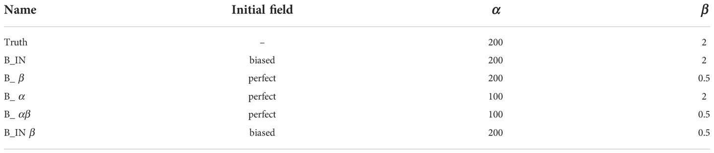
Table 1 Design of identical twin experiment, where “Truth” indicate the truth experiment, and “B_IN”, “B_ β “, “B_ α “ “B_ αβ “, and “B_IN β “ indicate the bias coming from initial field, β, α, both α and β, and initial field together with β, respectively.

In this study, when only one optimization algorithm is used, steps (5) and (6) or (7) and (8) are directly omitted.

Correctness test of the gradient of the cost function, TLM, and ADM

The correctness of the gradient of the cost function and TLM can be checked through the following formula respectively:

$\begin{array}{ll}\phi (ϵ)=\frac{J\left(x_0+\frac{ϵ\nabla J}{\Vert \nabla J\Vert }\right)-J\left(x_0\right)}{ϵ\Vert \nabla J\Vert }\approx 1,& (27)\end{array}$

$\begin{array}{ll}\phi (ϵ)=\frac{\Vert M(x_o+ϵh)-M(x_o)\Vert }{\Vert ϵ\mathbf{M}h\Vert }\approx 1.& (28)\end{array}$

Where x₀ is the control variable, h is the perturbation of x_o , the value of φ shall converge to 1 as ϵ tend to zero, ‖·‖ represents the two norm. Table 2 and Table 3 show the correctness of the gradient of the cost function and TLM with respect to α , β , and temperature initial field, respectively. For both of them, the φ(ϵ) convergence to around 1 as ϵ decrease from 10⁻² , and with the further reduction of ϵ , φ(ϵ) is far away from 1 due to the influence of calculation accuracy. From Table 2 and Table 3, one can see that the gradient and TLM of the initial field at least have a 7 digits accuracy, but two parameters in MY-2.5 turbulence enclosed scheme only 3 or 4 digits accuracy. The decrease in accuracy is mainly due to the direct linearization of a highly nonlinear and discontinuous turbulent kinetic energy scheme, which may produce nonphysical noise.

TABLE 2

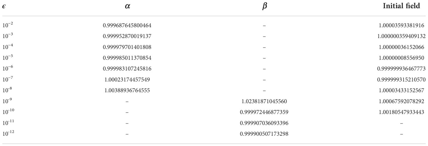
Table 2 The correctness test of the gradient of the cost function with respect to α, β, and initial field.

TABLE 3

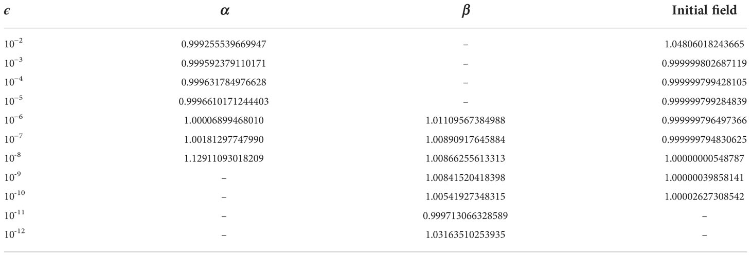
Table 3 The correctness test of the TLM with respect to α, β, and initial field.

The correctness check for ADM should satisfy the criteria:

$\begin{array}{ll}<\mathbf{M}h,\mathbf{M}h>=<{\mathbf{M}}^{\mathrm{T}}\mathbf{M}h,h>.& (29)\end{array}$

Where 〈·〉 represents the inner product. Here, for the whole POM concerning the initial field, the left-hand side is 0.144525709394330 and the right-hand side is 0.144525709394331. Equation (29) should be held with at least 13 digits of the left-hand side being the same as those of the right-hand side, so the accuracy satisfies the criteria. However, due to the high nonlinear and discontinuous of MY-2.5, α and β only 4 digits accuracy.

Truth simulation and biased simulation

POMgcs simulated the horizontal and profile structure of temperature and salt in winter and summer, respectively, based on the MY-2.5 parameterization scheme with the CB boundary. Figures 1, 2 show the results of the truth model simulation, where Figures 1A, B are the horizontal distribution of temperature and salt in January, respectively. Figures 1C, D are the same as Figures 1A, B, but for the profile distribution in 38.5^∘N . Figures 2A–D are the same as Figures 1A–D, but in August, respectively. One can see that the temperature and salt are uniformly mixed in the vertical in January. In August, the temperature formed a distinct thermocline in the area away from the coast, and the thickness of the upper mixing layer is about 10m. The water temperature at the bottom of the ocean remains cold as winter. However, the thermocline of salt is indistinctive. In winter, the horizontal construction of temperature shows that the closer it gets to the coast, the colder it gets, and the conclusion in summer is the opposite of that in winter. The above conclusions are consistent with those obtained from actual measured temperatures for many years (Su and Yuan, 2005). Therefore, this model is rational.

FIGURE 1

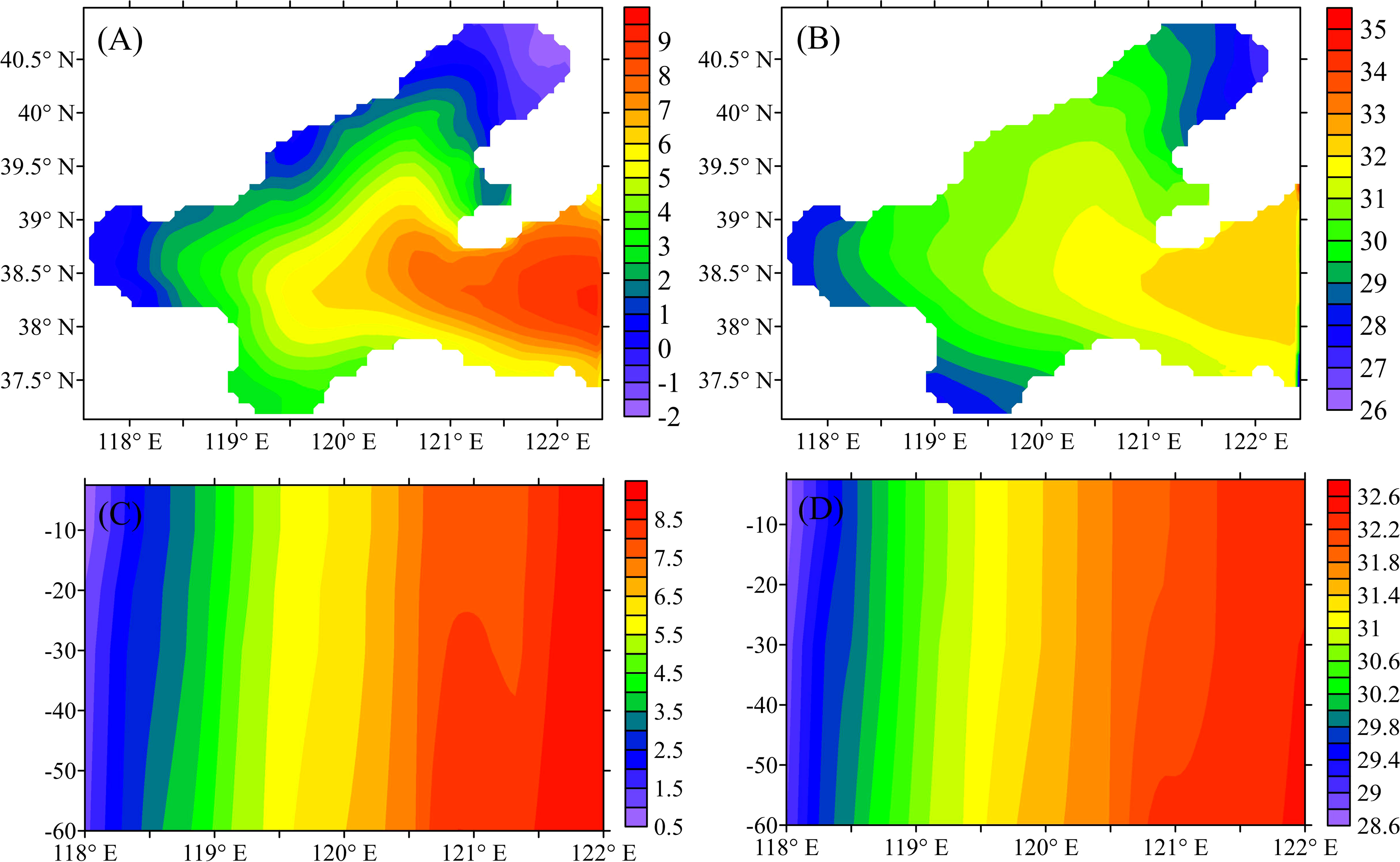
Figure 1 Simulated temperature (°C ) (A–C) and salt (B–D) horizontal (A, B) and 38.5^oN vertical (C, D) profile in January.

FIGURE 2

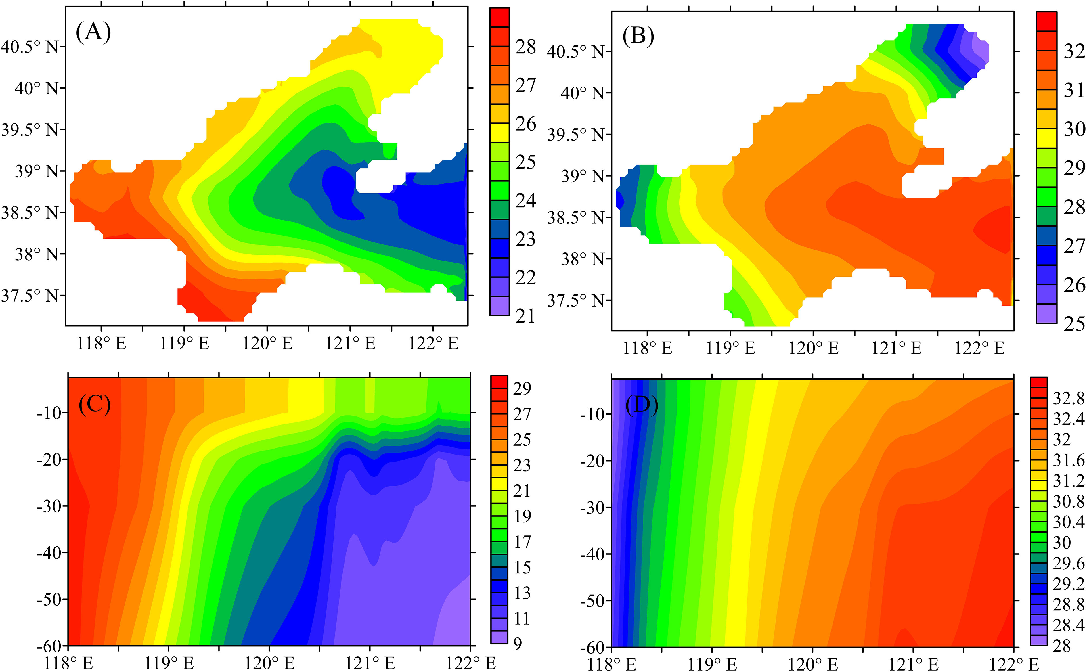
Figure 2 Simulated temperature (°C ) (A, C) and salt (B, D) horizontal (A, B)) and 38.5oN vertical (C, D) profile in August.

In this section, the biased simulation uses the model with biased wave-affected parameters, and the other configurations of the model are the same as the truth model. Comparing the biased simulation with perfect simulation aims to test the effect of incorrect parameters setting. Figure 3 shows the vertical structure of the difference in root-mean-square-error (RMSE) of the simulated temperature between the perfect model and the biased model with α=100 , β=0.5 in January. It can be seen that the difference in the temperature between the two simulations is pronounced at the sea surface and 10-m depth. This phenomenon is because the values of wave-affected parameters used in the biased model are smaller than that in the truth model, which indicates that the turbulent kinetic energy is too weak to mix the surface and subsurface water well in the biased simulation. Below 20m, the difference is tiny, suggesting that the turbulent kinetic energy generated by the breaking wave only affects near the sea surface and cannot penetrate the deeper sea. However, the wave-affected parameters play a vital role in the simulated upper layer structure of temperature. It is necessary to estimate the two parameters accurately.

FIGURE 3

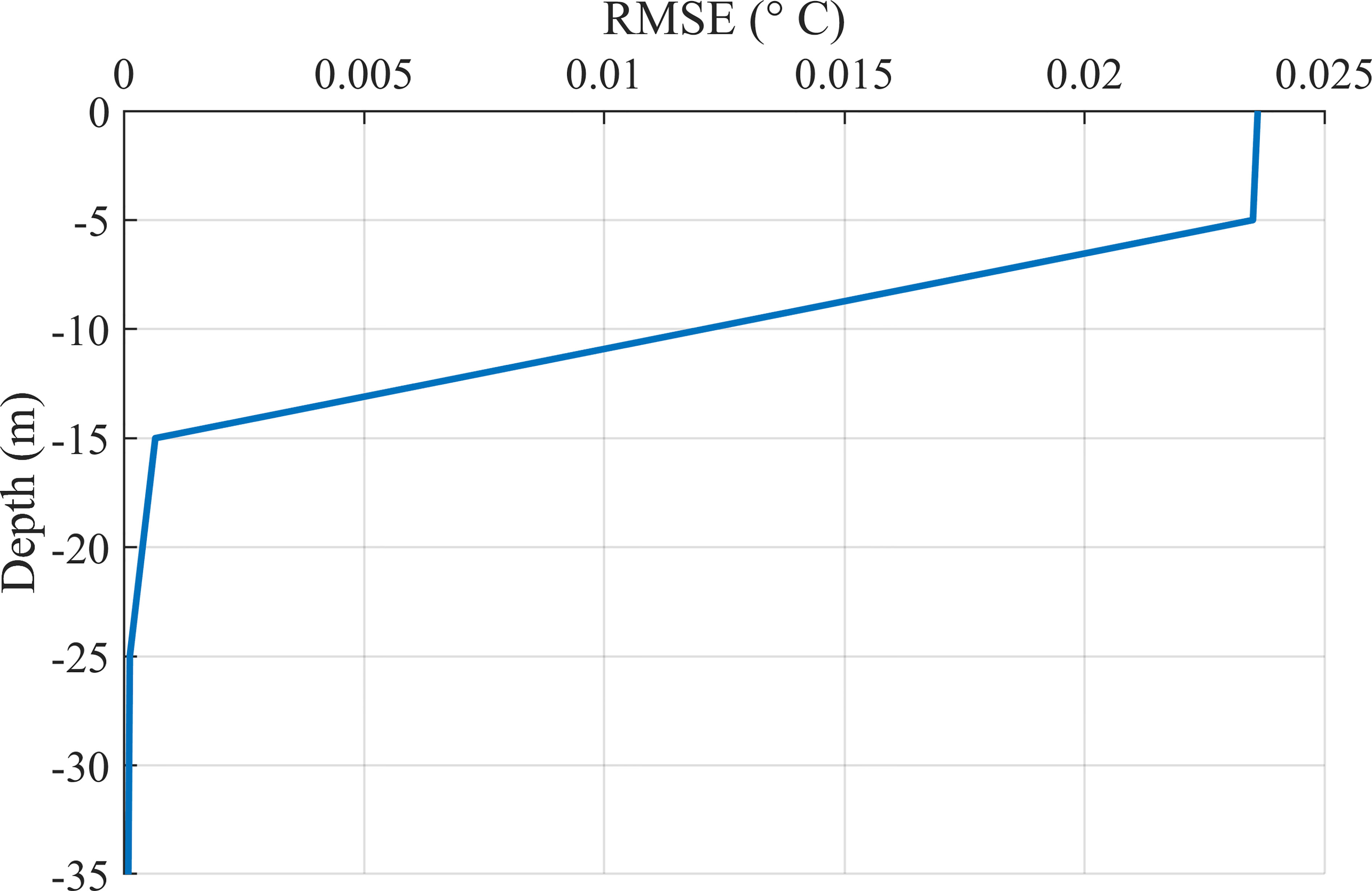
Figure 3 The vertical structure of the difference in RMSE of the temperature between the B_αβ and “truth” model simulation in January.

Initial field optimization

Figure 4 shows the variation of the cost function and norm of the gradient with several iterations for B_IN experiment. The value of the cost function decreases rapidly from 2810 to 0.045 within two iterations, and it keeps the low value (0.045) steadily after the second iteration (Figure 4A). Moreover, the norm of the gradient declines rapidly and then slightly oscillates to search for the optimal declining direction. The norm of the gradient nearly becomes stable after the 4^th iteration (Figure 4B), and the minimization process stops after 11 iterations, indicating the local minima of the initial field for that day.

FIGURE 4

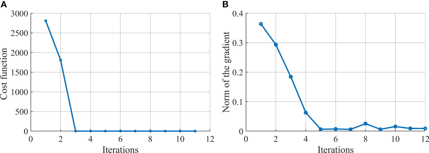
Figure 4 The variation of (A) the cost function and (B) the norm of the gradient with the number of iterations for B_IN experiment.

Figure 5 depicts the difference in temperature between the “truth” model simulation and biased initial field simulation without assimilation, and optimal initial field simulation with 4D-Var assimilation, respectively. It is evident that the temperature from the optimal initial field is closer to the “truth” simulation than that from a biased simulation. The above results show the usefulness of 4D-Var based on POMgcs for optimizing the initial field.

FIGURE 5

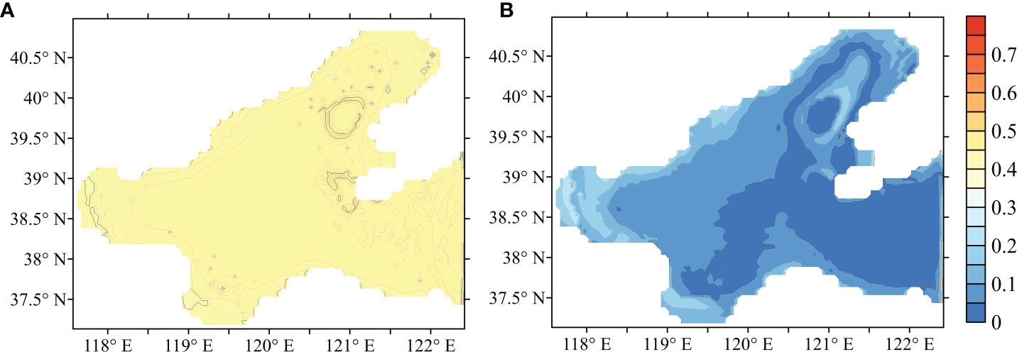
Figure 5 Temperature fields from the differences between (A) Truth and B_ IN, (B) Truth and optimal initial field simulation.

Sensitivity check

It is essential to investigate temperature sensitivities with respect to parameters being optimized before parameter estimation. Otherwise, if the insensitive physical variable to the parameter were used to perform parameter estimation, it would be hard to obtain an optimal solution. Figure 6 shows the distribution of the cost function with different α and β . One can see that it is increased with increasing parameters in general. However, the local minimum of the cost function is located in the region where α and β are closed to “truth” values (200 and 2). The existence of a local minimum indicates that it will probably estimate the optimal value of α and β if the gradient of the cost function can be calculated correctly through the ADM. However, α and β are not independent variables, the former represents the turbulence strength induced by the breaking-wave, and the latter is the influence range of turbulence, so the two parameters cannot be determined independently.

FIGURE 6

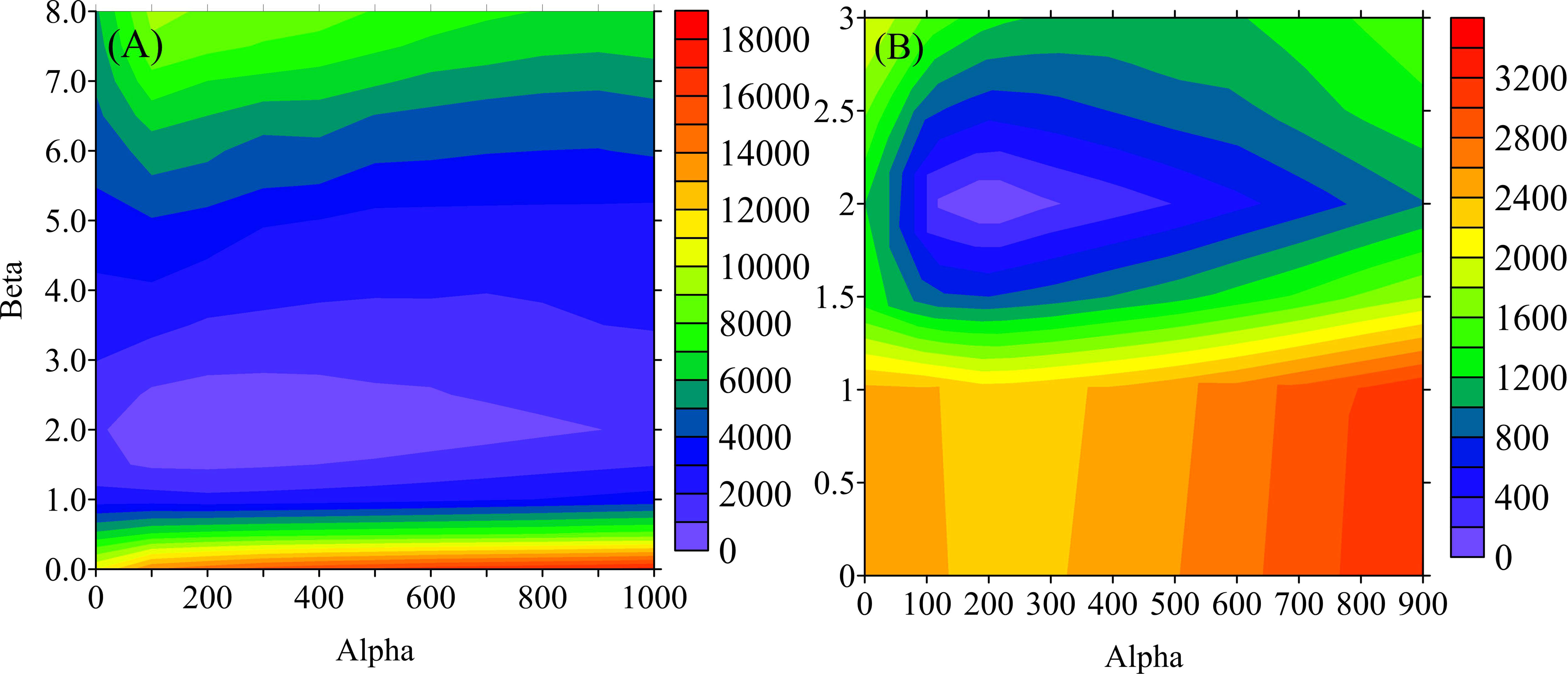
Figure 6 The value of the cost function on α and β for (A) 10≥β≥0 and (B) 3≥β≥0.

The gradient of the cost function with α and β can be used to investigate the model sensitivities with respect to the two parameters. Table 4 shows the value of the gradient with different parameters. The closer the value is to zero, the more sensitive it is to the corresponding parameter value. When the wave-affected parameters are exactly set to 200 and 2, respectively, both gradient values are the closest to zero. It can be found that the sensitivities value of β is several orders of magnitude greater than α. It indicates that α is more vulnerable to being disturbed by the error that arises from observation and initial field during parameter estimation.

TABLE 4

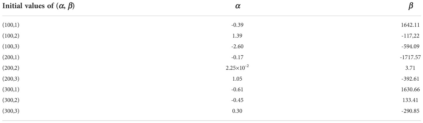
Table 4 Dependence of the sensitivity on the initial values of the parameters α and β.

Parameters estimation

In this section, B_α and B_β experiments are conducted to determine whether the wave-affect parameters can be estimated correctly or not, where the initial field is perfect. Figure 7 depicts the iteration variations of the cost function, norm of the gradient, and the value of the parameter when the control variable is α or β. Where the left side of Figure 7 shows B_α experiment result, and the other side is B_β . When the control variable is only α, both the cost function and the norm of the gradient decrease dramatically in the first four iterations and keep stable after the 5^th iteration, the wave-affected parameter α from the initial value of 0.5 converges to the “truth” value within 6 times iterations with the 4D-Var method, while β from the initial value of 100 converges to its “truth” value after about 4 times iterations.

FIGURE 7

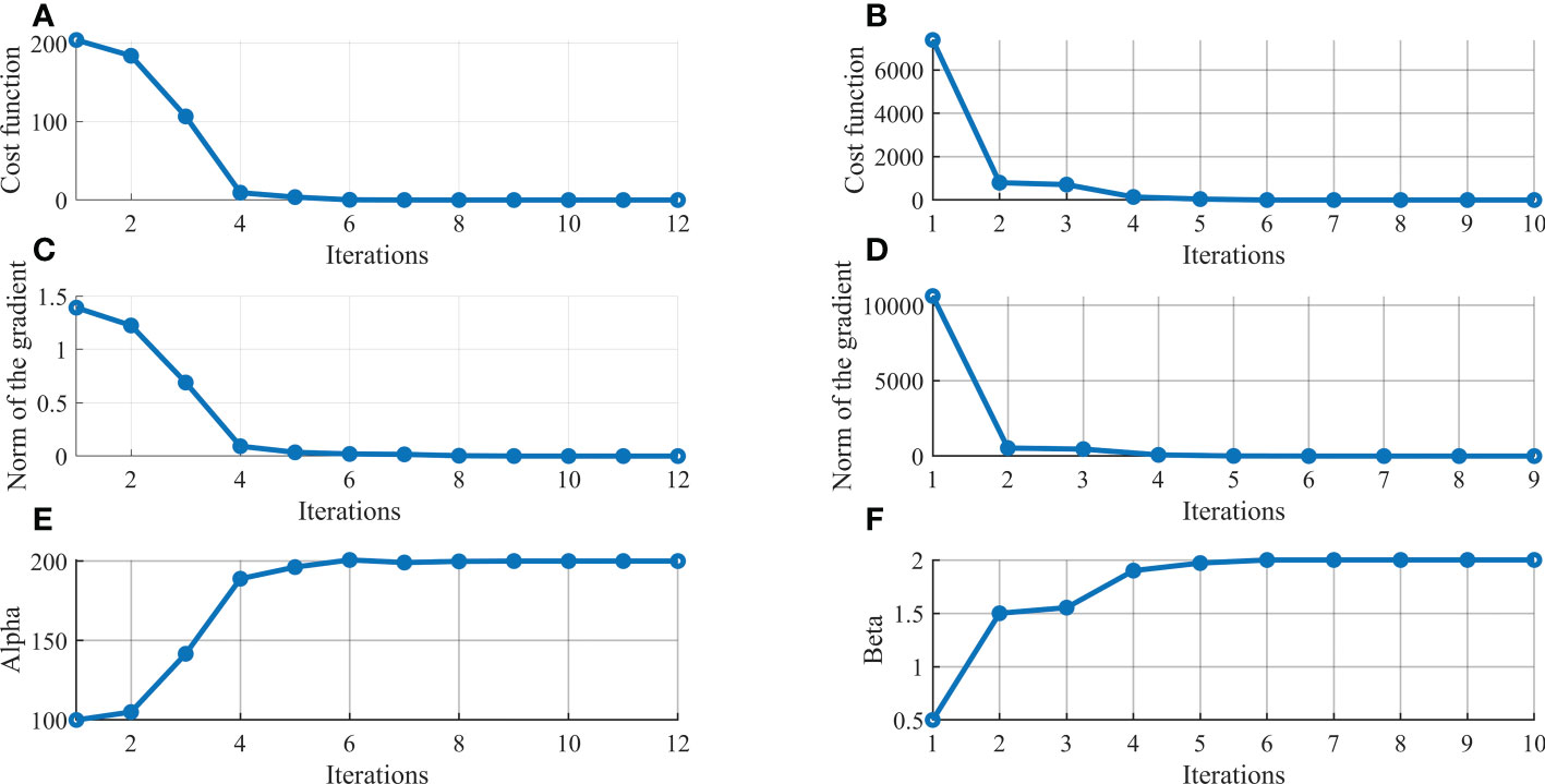
Figure 7 The variation of the cost function, the norm of the gradient, and the value of the wave-affected parameter with the number of iterations for B_ α (A, C, E) and B_ β (B, D, F) experiment, respectively.

Figure 8 shows the variation of the cost function, the norm of the gradient, and two wave-affected parameters with the number of the iterations for B_αβ experiment, where only LBFGS algorithms is used. Due to the nonlinearity of the model, the cost function is not strictly convex, and a nonconvex cost function may have many local minimums. The parameter estimation strongly relies on the initial value of the parameter. Under this condition, when both wave-affected parameters are selected as the control variables, neither α nor β reaches their “truth” value. In this study, the two optimization algorithms LBFGS and LMBM, are applied to enhance the estimation of the double parameters. LBFGS is suitable for solving large-scale optimization problems but has not been proved to be globally convergent for nonconvex or nonsmooth cost functions (Haarala et al., 2007). LMBM combines the variable metric bundle method and the limited memory variable metric method. It is not only suitable for solving large-scale nonsmooth but also globally convergent for nonconvex unconstrained optimization problems. The utilization of the two optimization algorithms speeds up the convergence as well as probably jumps out the local extremum near the initial value of the parameters, thus the parameters are more likely to converge to the “truth” value. Figures 9A, B shows the iteration series of the cost function with the LMBM and LBFGS, respectively. It can be found that the cost function dramatically oscillates in the beginning and becomes stable from the ninth cycle with LMBM method, and then, with LBFGS, it continues decreasing until converging to 0. Figures 9C–F depicts the variation of the wave-affected parameters with LMBM and LBFGS algorithms. One can see that α remarkably boost from the 5^th to 9^th iteration, then decrease and tend to be stable. However, the parameter failed to converge to the “truth” value with a single optimization algorithm. As shown in Figure 9D, optimizing the cost function with the LBFGS algorithm, α gradually reaches the truth value. The evolution of the value of β with the number of iterations is similar to that of α.

FIGURE 8

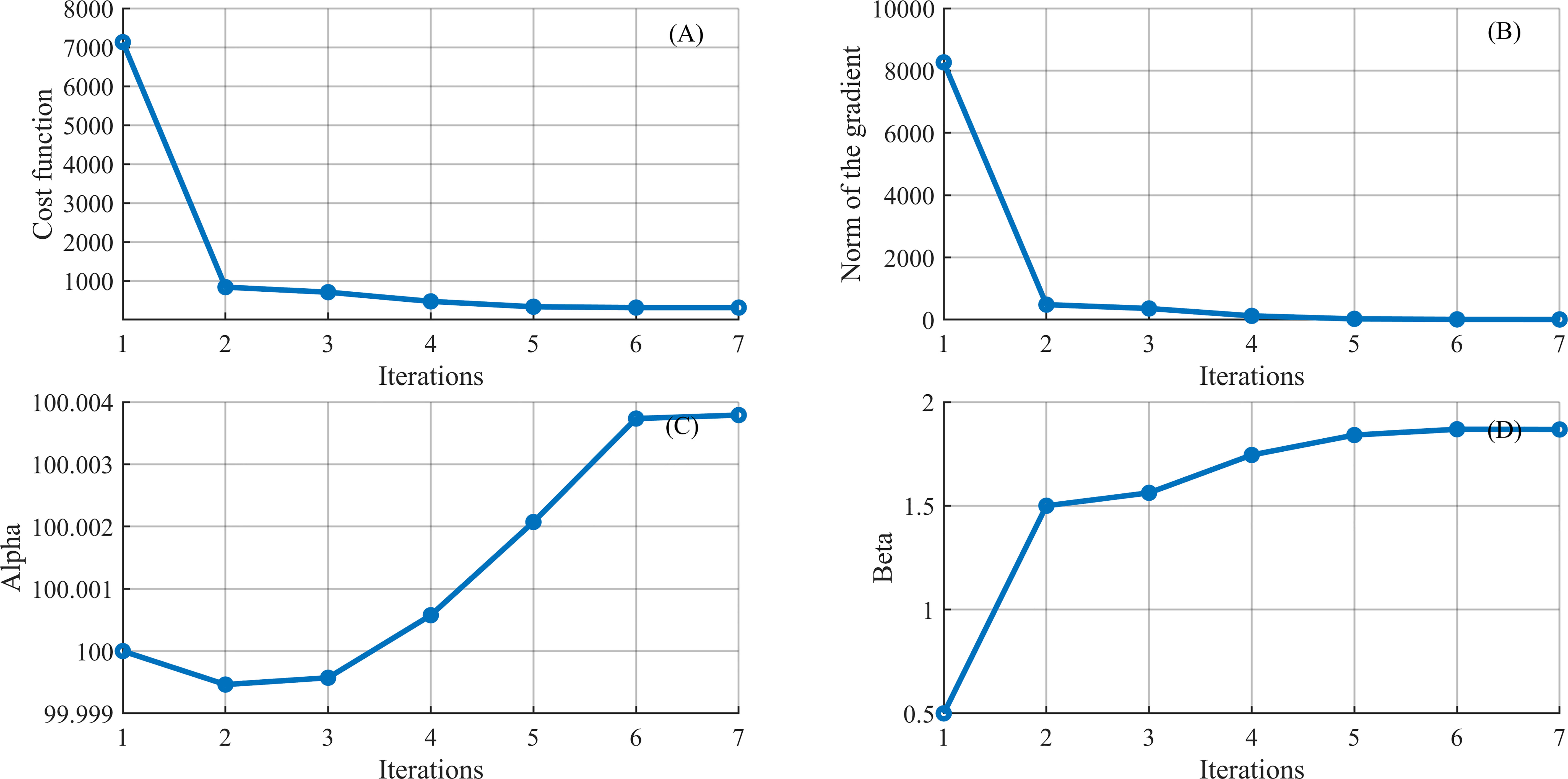
Figure 8 The variation of (A) the cost function, (B) the norm of the gradient, and wave-affected parameters (C) α and (D) β with LBFGS for B_αβ experiment.

FIGURE 9

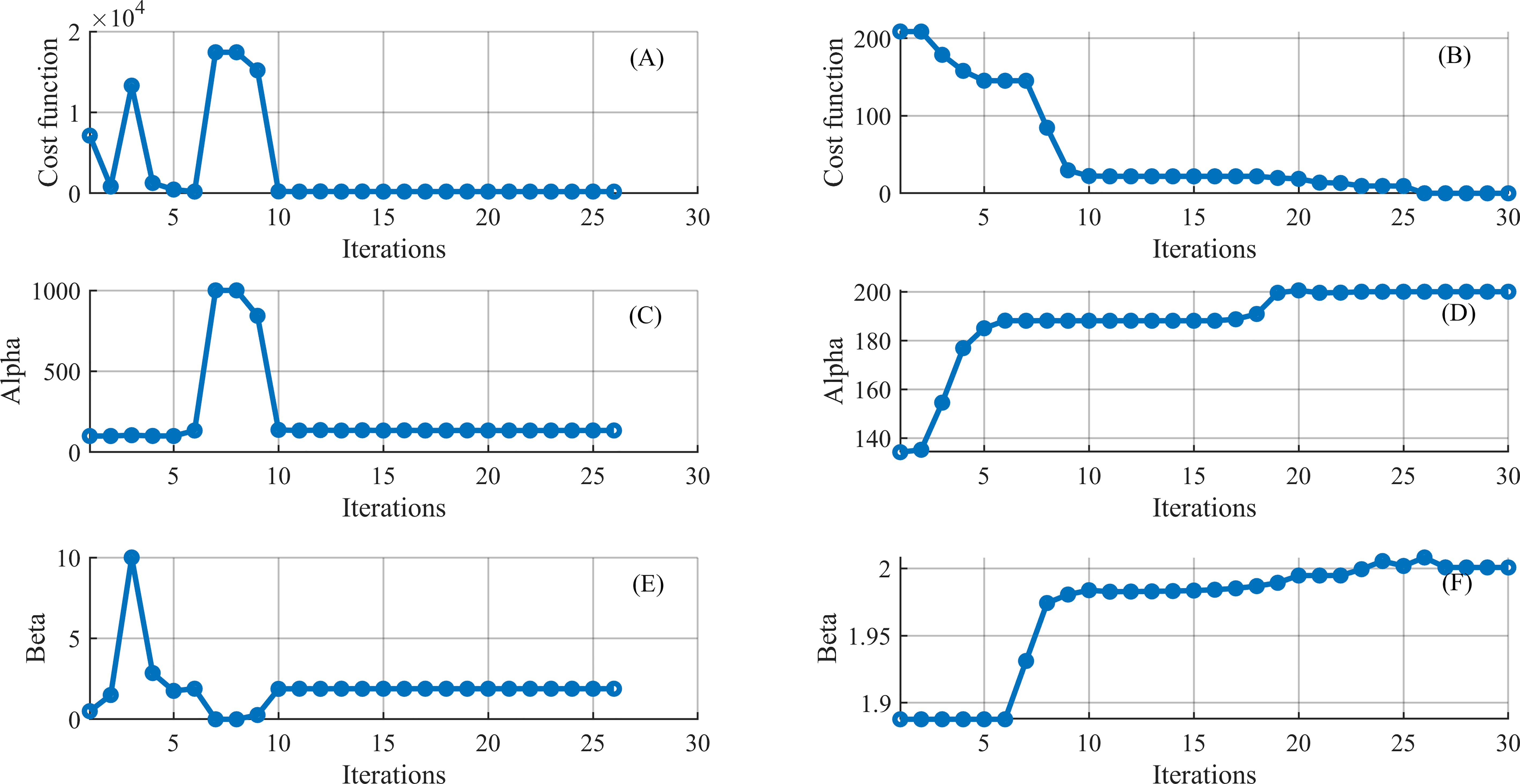
Figure 9 The evolution of the cost function, α, and β with LMBM (A, C, E) and LBFGS (B, D, F) for B_αβ experiment, respectively.

When the initial condition and parameter are regarded as control variables simultaneously, the accuracy of the parameter estimation is restricted by that of the state estimated. In this case, the parameter hardly reaches the “truth” value and merely attains the optimal value of the parameter to compensate for the error derived from the state variable. Figure 10 shows the B_INβ experiment result. It can be found that β does not converge to the “truth” value even though two optimal algorithms are used. However, β has almost reached the optimal value close to the truth value from the eighth iteration with LMBM.

FIGURE 10

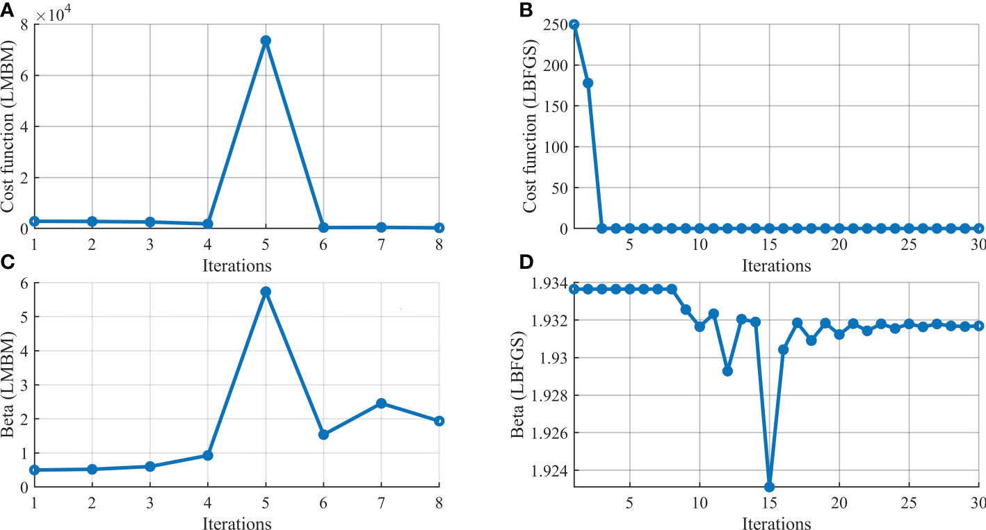
Figure 10 The evolution of (A, B) the cost function and (C, D) β value with LMBM and LBFGS algorithms for B_IN β experiment, respectively.

Figure 11 depicts the evolution of parameters α and β based on B_α and B_β with the number of iterations when their initial values are set to (50, 150, 250, 300) and (1, 1.5, 2.5, 3), respectively. It clearly shows that the parameters converge to the “truth” value no matter what the initial values are. Therefore, the 4D-Var based on 3D-POMgcs is feasible for one wave-affected parameter estimated with different initial parameter values and the perfect initial field.

FIGURE 11

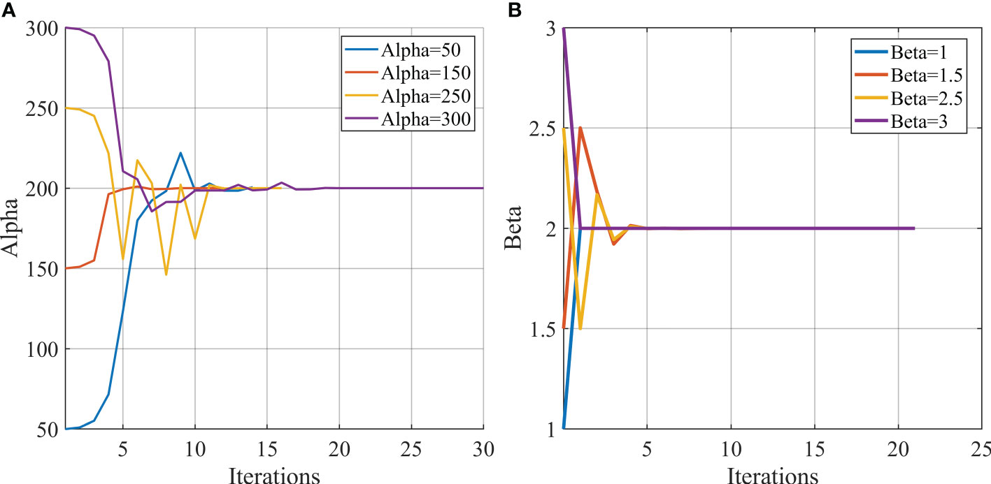
Figure 11 The evolution of the estimated wave-affected parameters (A) α and (B) β for different initial values with the number of iterations.

To investigate the impact of the temperature observation noise on wave-affected parameters, the next experiment is designed based on B_β and B_α, and adds different standard deviation noises into temperature observation. Table 5 shows the dependence of parameter estimation on the standard deviation of temperature observation. The relative error is obtained by the absolute error divided by the true value (i.e. the greater the relative error, the lower the reliability). One can see from the table that the relative error increases with increasing the standard deviation. When the standard deviation exceeds 0.5, both reliabilities of α and β are quite low, which indicates the noise level is not acceptable for assimilation purposes. However, the variation of the relative error of β is more slowly than that of α as the standard deviation goes up. In other words, the effect of observational noise on the estimation is more severe on α than on β, which means the positive signal of α is difficult to capture during the optimization process, when the noise dominates the model and observation.

TABLE 5

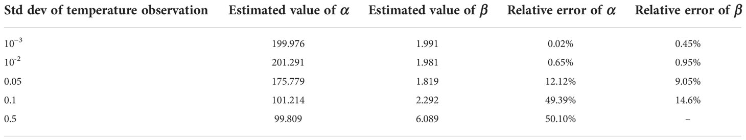
Table 5 Dependence of the optimally estimated on the standard deviation of the temperature observation.

Forecast experiment

A 72-h forecast of the upper 35m level temperature is performed with the optimal initial field and parameter from the 4D-Var algorithms. In the forecast experiment, the error source is the initial field and β parameter, where the initial field is obtained by adding 0.35 perturbation to “truth” value, and β parameter is set as 0.3. Since α is more susceptible than β to error from observation or initial field, when both α and β are taken as control variables, there is almost no improvement in α, so only parameter β is involved in this experiment. The control variable is the initial temperature field for the first forecast experiment (EINP-IN). For another forecast experiment (EINP-INP), the initial temperature field and β parameter are optimized simultaneously. A control run with a biased initial field and β parameter without assimilation is called control (CTRL). In these forecast experiments, the assimilation window, assimilation period, and observation source are the same as the assimilation experiments mentioned in the above section. The analysis result of assimilation is used as the initial field and parameter for the 72-h sea temperature forecast.

The RMSE of the 72-h forecast of the sea temperature with respect to the corresponding “truth” value for CTRL, EINP-IN, and EINP-INP is shown in Figures 12, 13. Figure 12 depicts the time series of RMSE of sea surface temperature (SST) starting from 01Z January 01 to 02Z January 04 for three experiments. Compared to CTRL, significant improvements can be seen in EINP-IN and EINP-INP, with EINP-INP outperforming EINP-IN because β reached 2.09 in EINP-INP, which is more close to the truth value. Figure 13 is the same as Figure 12, but for the 35m level. Similar results are found at the 35m level, but in the first few hours, the advantage of the EINP-INP over EINP-IN is not obvious. In the 35m depth, the RMSE of the initial field for the 72-h forecast is 0.1488 and 0.1486 for EINP-IN and EINP-INP, respectively. However, that is 0.2233 and 0.1531 on the sea surface, respectively. This is due to the fact that the breaking wave has a more significant impact on the sea surface than on the deep sea, and the biased parameter leads to larger RMSE of analysis results on the sea surface than at the 35m levels. With the accumulation of initial field and parameter error, the advantage of EINP-INP is shown after three hours at the 35m level. Figure 14 shows the vertical structure of the vertical mixed coefficient KH for EINP-IN and EINP-INP. The simulated averaged vertical mixing coefficient for temperature are much larger for the upper-15-m layer in EINP-INP than in EINP-IN. Below 15m, KH obtained by EINP-INP is still slightly larger than that obtained by EINP-IN, due to too low turbulent mixing strength, the improvement is not shown in Figure 14. The increased KH indicate the enhanced of turbulent mixing strength, which make the seawater of upper layer more vertically homogeneous, so the model performance can be effectively improved by EINP-INP.

FIGURE 12

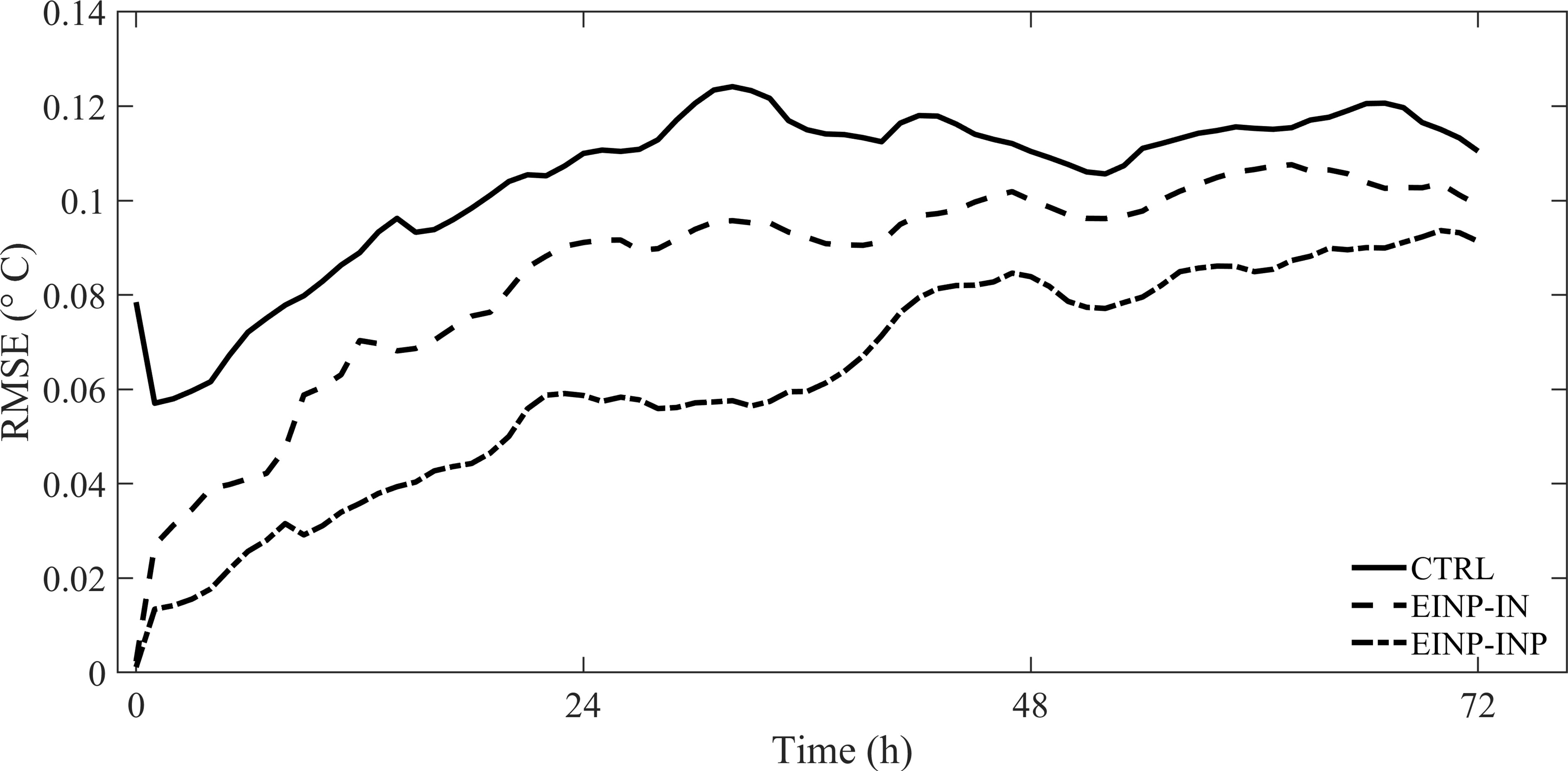
Figure 12 The RMSE of 72-h forecast of surface temperature with respect to “truth” value for CTRL, EINP-IN, and EINP-INP.

FIGURE 13

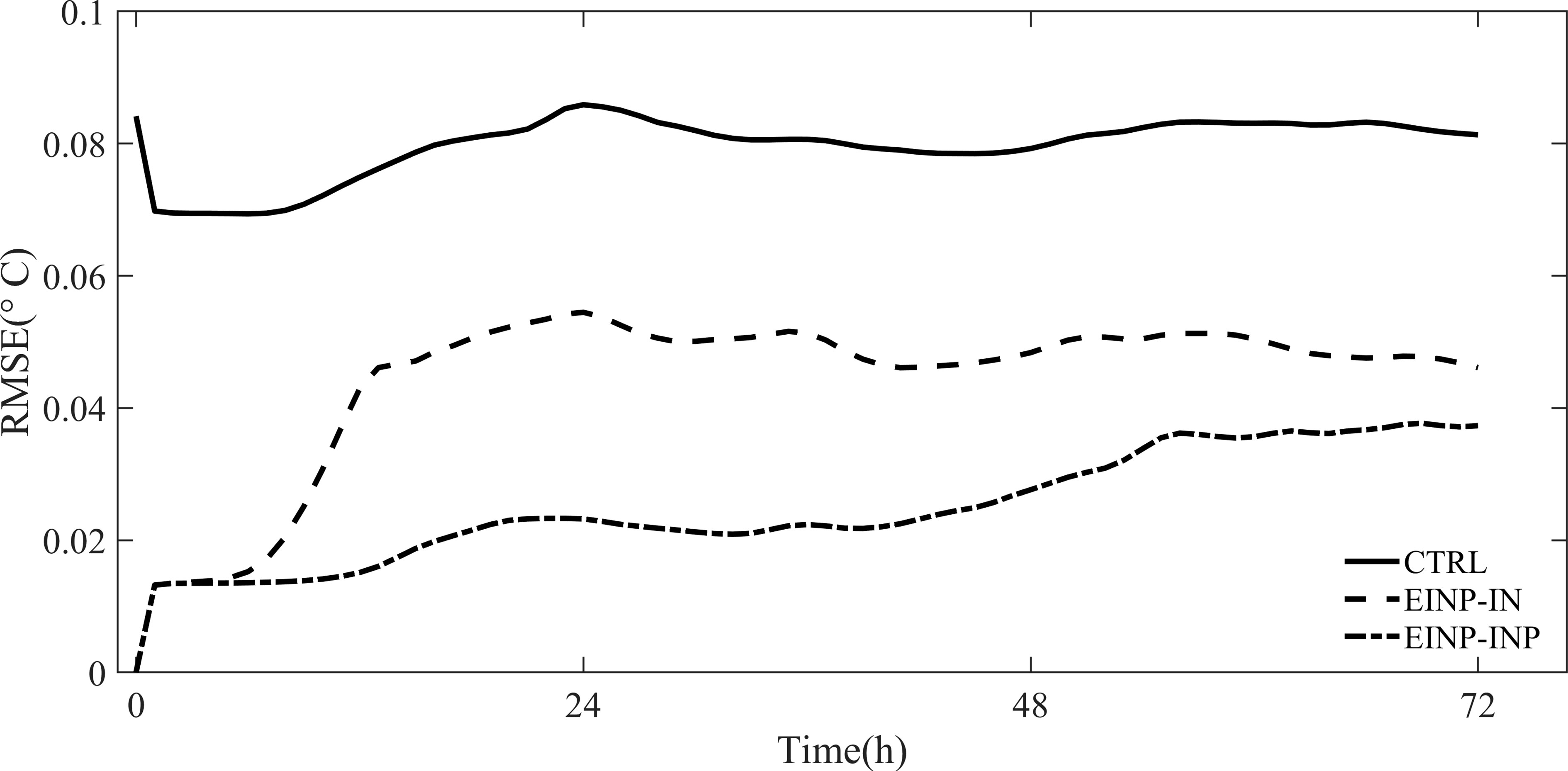
Figure 13 As in Figure 12, but for 35m levels.

FIGURE 14

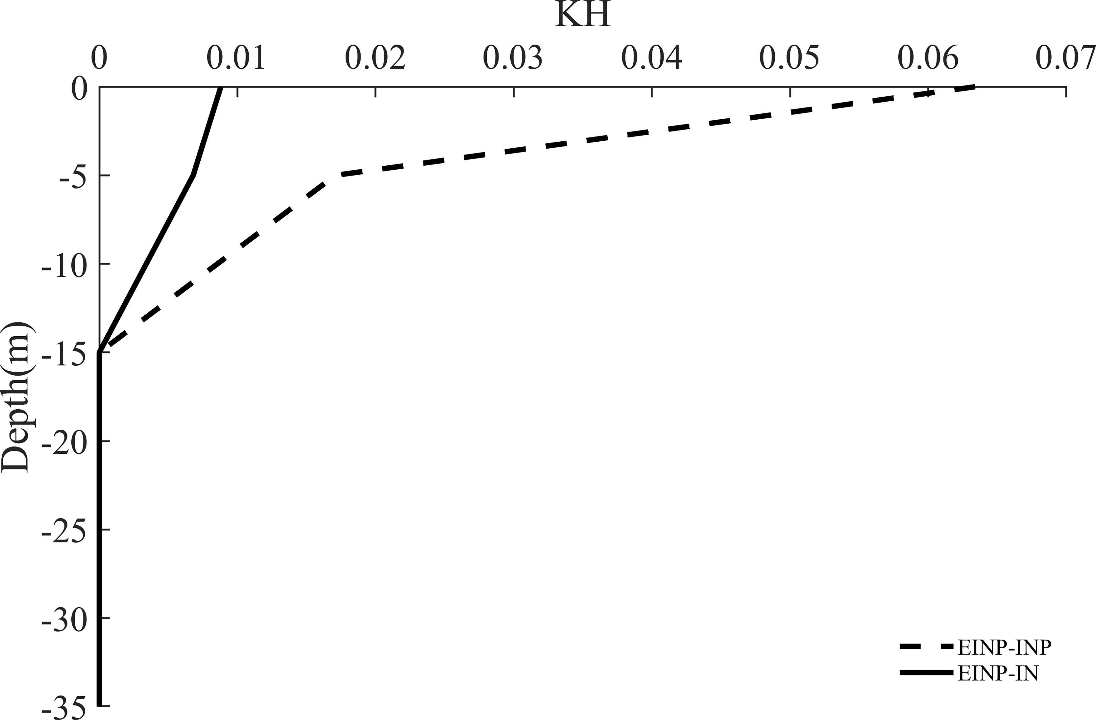
Figure 14 Vertical profiles of the simulated averaged the vertical mixing coefficient for temperature KH (m² s^-2) from EINP-IN and EINP-INP.

Summary and discussion

In this study, the three-dimensional and complete ADM of POMgcs is developed to build 4D-Var. Due to the high nonlinear and discontinuity of the vertical of the MY-2.5 turbulence enclosed scheme, nonphysical noise might be produced and then lead to the numerical oscillation during linearizing it. Although developing the adjoint code is complex, the effective and robust ADM has been obtained by TAMC and hand-coding correction. To evaluate the feasibility of the 4D-Var based on POMgcs with the MY-2.5, the two uncertain parameters in the MY-2.5 parameterization scheme, wave energy factor α and Charnock coefficient β, are tentatively estimated via the 4D-VAR algorithm. The two wave-affected parameters determine the magnitude and effective depth of turbulent kinetic energy, respectively. The turbulence kinetic energy can modulate the vertical structure distinctly in the upper ocean, the dissipation of which is adjusted by surface gravity waves under breaking waves. In order to investigate the upper ocean mixed layer, it is essential to obtain the optimal value of the wave-affect parameters in the turbulence-closed scheme.

First of all, the distribution of the temperature and salinity in Bohai is simulated by POMgcs for evaluating the rationally of the MY-2.5 turbulence enclose scheme. Based on that, the “truth model” and “pseudo-observations” are constructed for the following identical twin experiment. After thoroughly testing the capability of the 4D-Var for optimizing the initial field, a suite of parameter estimation experiments is performed. Within an identical twin experiment framework, when the single parameter is being optimized, the “truth” value of the wave-affected mixing parameters can be estimated successfully, no matter what the value of the initial parameter is. However, when the two parameters are used as the control variable simultaneously, the parameters fail to reach the “truth” value with the LBFGS optimization algorithm. In this study, both LMBM and LBFGS optimization algorithms are used within one assimilation period, which can speed up the convergence and jump out the local minimum of the cost function. When both the initial field and wave-affected are set to the control variable, parameter estimation is limited by the accuracy of the initial field. In that case, the parameter cannot converge to the “truth” value. However, 4D-Var can fit the model results to the observations, and the optimal value of the parameter can be estimated to compensate for part of the error arising from the initial field of the numerical model. Furthermore, the wave-affected parameter can also reach the optimal value when the observation error is acceptable. It is worth noting that α is more susceptible than β to error from observation or initial field. When α and the initial field are optimized, the parameter cannot converge to an optimal value, even if LMBM and LBFGS algorithms are used simultaneously. The 4D-Var algorithm aims to obtain an ‘optimal’ initial field or parameter for a better forecast. Therefore, the forecast experiment is performed to further demonstrate 4D-Var, where the forecast errors are attributed to incorrect initial fields and parameters. The results indicate that optimizing both of them or the initial field by setting them as control variables is effective for 4D-Var to improve sea temperature simulation, whether sea surface or deep sea and adjusting the initial field and parameter outperforms only the initial field.

The above results imply that the complete ADM of POMgcs developed in this study is feasible. However, since the precision of the TLM, ADM, and gradient of the cost function for the two parameters is lower due to the high nonlinearity of the MY-2.5, the optimization of α and β is more suitable for short integration time. The process of parameter optimization is not only model-dependent but also observation-dependent. It is well known that high-frequency observations are essential for the study of turbulence. In the real observation experiment, the ability of parameter optimization can be improved by high-frequency observations from surface drifting buoys, in situ subsurface buoy, etc. Thus more observations can be assimilated into the model in less integration time. In addition, reducing the initial field error is essential for obtaining the “optimal” α, a more comprehensively designed background error covariance based on flow-dependent or multiscale may enhance the effectiveness of the initial field. These will be explored in our further studies.

Data availability statement

The raw data supporting the conclusions of this article will be made available by the authors, without undue reservation.

Author contributions

Conceptualization: XZ, YH. Methodology: YH, XZ. Software: XZ, YH. Formal analysis: YH. Writing-original draft: YH. Writing – review & editing: WL, XZ. All authors contributed to the article and approved the submitted version.

Funding

This research was funded by grants from the National Key Research and Development Program (2021YFC3101501) and the National Natural Science Foundation (41876014) of China.

Conflict of interest

The authors declare that the research was conducted in the absence of any commercial or financial relationships that could be construed as a potential conflict of interest.

Publisher’s note

All claims expressed in this article are solely those of the authors and do not necessarily represent those of their affiliated organizations, or those of the publisher, the editors and the reviewers. Any product that may be evaluated in this article, or claim that may be made by its manufacturer, is not guaranteed or endorsed by the publisher.

References

Andersson E., Pailleux J., The´paut J.-N., R Eyre J., McNally A. P., Kelly G. A., et al. (1994). Use of cloud-cleared radiances in three/four-dimensional variational data assimilation. Quart. J. R. Meteor. Soc 120, 627–653. doi: 10.1002/qj.49712051707

CrossRef Full Text | Google Scholar

Bennett A. F., McIntosh P. C. (1982). Open ocean modeling as an inverse problem: tidal theory. J. Phys. Oceanogr. 12, 1004–1018. doi: 10.1175/1520-0485(1982)012<1004:OOMAAI>2.0.CO;2

CrossRef Full Text | Google Scholar

Blumberg A., Mellor G. (1987). A description of a three dimensional coastal ocean circulation model. Three-dimensional coastal ocean models. Coast. Estuar. Sciences Amer. Geophys. Union 4, 1–16. doi: 10.1029/CO004-p0001

CrossRef Full Text | Google Scholar

Bouttier F., Courtier P. (1999). Data assimilation concepts and methods. meteorological training course lecture series. Printed January 9 2001, 33–35.

Google Scholar

Courtier P., The´paut J.-N., Hollingsworth A. (1994). A strategy for operational implementation of 4D-var, using an incremental approach. Quart. J. R. Meteor. Soc 120, 1367–1388. doi: 10.1002/qj.49712051912

CrossRef Full Text | Google Scholar

Craig P. D. (1996). Velocity profiles and surface roughness under wave breaking. J. Geophys. Res. 101, 1265–1277. doi: 10.1029/95JC03220

CrossRef Full Text | Google Scholar

Craig P. D., Banner M. L. (1994). Modeling wave-enhanced turbulence in the ocean surface layer. J. Phys. Oceanogr. 24, 2546–2559. doi: 10.1175/1520-0485(1994)024,2546:MWETIT.2.0.CO;2

CrossRef Full Text | Google Scholar

Das S. K., Lardner R. W. (1991). On the estimation of parameters of hydraulic models by assimilation of periodic tidal data. J. Geophys. Res. 96, 15187–15196. doi: 10.1029/91JC01318

CrossRef Full Text | Google Scholar

Ezer T., Mellor G. L. (2004). A generalized coordinate ocean model and a comparison of the bottom boundary layer dynamics in terrain-following and in z-level grids. Ocean Modell. 6, 379–403. doi: 10.1016/S1463-5003(03)00026-X

CrossRef Full Text | Google Scholar

Galperin B., Kantha L. H., Hassid S., Rosati A. (1988). A quasi-equilibrium turbulent energy model for geophysical flows. J. Atmos. Sci. 45, 55–62. doi: 10.1175/1520-0469(1988)0452.0.CO;2

CrossRef Full Text | Google Scholar

Giering R., Kaminski T. (1998). Recipes for adjoint code construction. ACMTrans. Math. Software 24, 437–474. doi: 10.1145/293686.293695

CrossRef Full Text | Google Scholar

Haarala N., Miettinen K., Mäkelä M. M. (2004). New limited memory bundle method for large-scale nonsmooth optimization. Optim. Methods Softw 19, 673–692. doi: 10.1080/10556780410001689225

CrossRef Full Text | Google Scholar

Haarala N., Miettinen K., Mäkelä M. M. (2007). Globally convergent limited memory bundle method for large-scale nonsmooth optimization. Math. Program 109, 181–205. doi: 10.1007/s10107-006-0728-2

CrossRef Full Text | Google Scholar

Heemink A. W., Mouthaan E. E. A., Roest M. R. T., Vollebregt E. A. H., Robaczewska K. B., Verlaam M. (2002). Inverse 3D shallow water flow modeling of the continental shelf. Continental Shelf Res. 22, 465–484. doi: 10.1016/S0278-4343(01)00071-1

CrossRef Full Text | Google Scholar

Lardner R. W., Song Y. (1995). Optimal estimation of eddy viscosity and friction coefficients for a quasi-three-dimensional numerical tidal model. Atmos.-Ocean 33, 581–611. doi: 10.1080/07055900.1995.9649546

CrossRef Full Text | Google Scholar

LeDimet F. X., Talagrand O. (1986). Variational algorithms for analysis and assimilation of meteorological observations: theoretical aspects. Tellus 38A, 97–110. doi: 10.1111/j.1600-0870.1986.tb00459.x

CrossRef Full Text | Google Scholar

Liu D. C., Nocedal J. (1989). On the limited memory BFGS method for large scale optimization. Math. Program 45, 503–528. doi: 10.1007/BF01589116

CrossRef Full Text | Google Scholar

Lu J., Hsieh W. E. (1997). Adjoint data assimilation in coupled atmosphere–ocean models: determining initial model parameters in a simple equatorial model. Quart. J. R. Meteor. Soc 123, 2115–2139. doi: 10.1002/qj.49712354316

CrossRef Full Text | Google Scholar

Lu J., Hsieh W. E. (1998a). Adjoint data assimilation in coupled atmosphere–ocean models: determining initial conditions in a simple equatorial model. J. Meteor. Soc Jpn. 76, 737–748. doi: 10.2151/jmsj1965.76.5_737

CrossRef Full Text | Google Scholar

Lu J., Hsieh W. E. (1998b). On determining initial conditions and parameters in a simple couples atmosphere–ocean model by adjoint data assimilation. Tellus 50A, 534–544. doi: 10.1034/j.1600-0870.1998.00011.x

CrossRef Full Text | Google Scholar

Mellor G. L. (1989). “Retrospect on oceanic boundary layer modeling an second moment closure,” in Hawaiian Winter workshop on "Parameterization of small-scale processes" (Honolulu, Hawaii: University of Hawaii).

Google Scholar

Mellor G. L. (2002). Users guide for a three-dimensional, primitive equation, numerical ocean model. Prog. Atmos. Ocean. Sci.. Princeton Univ. 17 (1), 4–42.

Google Scholar

Mellor G. L., Yamada T. (1982). Development of a turbulence closure model for geophysical fluid problems. Rev. Geophys. Space Phys. 20, 851–875. doi: 10.1029/RG020i004p00851

CrossRef Full Text | Google Scholar

Navon I. M., Zou X., Derber J., Sela J. (1992). Variational data assimilation with an adiabatic version of the NMC spectral model. Mon.Weather Rev. 120, 1433–1446. doi: 10.1175/1520-0493(1992)1202.0.CO;2

CrossRef Full Text | Google Scholar

Peng S. Q., Xie L. (2006). Effect of determining initial conditions by four-dimensional variational data assimilation on storm surge forecasting. Ocean Modell. 14, 1–18. doi: 10.1016/j.ocemod.2006.03.005

CrossRef Full Text | Google Scholar

Peng S.-Q., Zou X. (2002). Assimilation of NCEP multi-sensor hourly rainfall data using 4D-var approach: a case study of the squall line on April 5 1999. Meteor. Atmos. Phys. 81, 237–255. doi: 10.1007/s00703-002-0545-y

CrossRef Full Text | Google Scholar

Peng S.-Q., Zou X. (2004). Assimilation of ground-based GPS zenith total delay and rain gauge precipitation observations using 4D-var and their impact on short-range QPF. J. Meteor. Soc Jpn. 82, 491–506. doi: 10.2151/jmsj.2004.491

CrossRef Full Text | Google Scholar

Peng S.-Q., Xie L., Pietrafesa L. J. (2007). Correcting the errors in the initial conditions and wind stress in storm surge simulation using an adjoint optimal technique. Ocean Modell 18, 175–193. doi: 10.1016/j.ocemod.2007.04.002

CrossRef Full Text | Google Scholar

Peng S.-Q., Li Y., Xie L. (2013). Adjusting the wind stress drag coefficientin storm surge forecasting using an adjoint technique. J. Atmos. Oceanic Technol. 30, 590–608. doi: 10.1175/JTECH-D-12-00034.1

CrossRef Full Text | Google Scholar

Qiao F., Yuan Y., Yang Y., Zheng Q., Xia C., Ma J. (2004). Wave-induced mixing in the upper ocean: distribution and application to a global ocean circulation model. Geophysical Res. Lett. 31, L11303. doi: 10.1029/2004GL019824

CrossRef Full Text | Google Scholar

Rabier F., Courtier P. (1992). Four-dimensional assimilation in the presence of baroclinic instability. Quart. J. R. Meteor. Soc 118, 649–672. doi: 10.1002/qj.49711850604

CrossRef Full Text | Google Scholar

Robert A. J. (1966). The integration of a low-order spectral form of the primitive meteorological equations. J. Meteor. Soc Japan 44, 237–245. doi: 10.2151/jmsj1965.44.5_237

CrossRef Full Text | Google Scholar

Sasaki Y. (1970). Some basic formalisms in numerical variational analysis. Mon. Weather Rev. 98, 875–883. doi: 10.1175/1520-0493(1970)098<0875:sbfinv>2.3.co;2

CrossRef Full Text | Google Scholar

Seiler U. (1993). Estimation of open boundary conditions with the adjoint method. J. Geophys. Res. 98, 22855–22870. doi: 10.1029/93jc02376

CrossRef Full Text | Google Scholar

Su J. L., Yuan L. Y. (2005). China Offshore hydrology (Beijing: Ocean Press).

Google Scholar

Talagrand O., Courtier P. (1987). Variational assimilation of meteorological observations with the adjoint vorticity equation. part I: Theory. Quart. J. R. Meteor. Soc 113, 1311–1328. doi: 10.1002/qj.49711347812

CrossRef Full Text | Google Scholar

Terray E. A., Donelan M. A., Agarwal Y., Drennan W. M., Kahma K., Williams A. J. III, et al. (1996). Estimates of kinetic energy dissipation under breaking waves. J. Phys. Oceanogr. 26, 792–807. doi: 10.1175/15200485(1996)026,0792:EOKEDU.2.0.CO;2

CrossRef Full Text | Google Scholar

Terray E. A., Drennan W. M., Donelan M. A.. (1999). The vertical structure of shear and dissipation in the ocean surface layer. In Banner M. L. Ed. The Wind-Driven Air-Sea Interface: Electromagnetic and Acoustic Sensing, Wave Dynamics and Turbulent Fluxes University of New South Wales, 239–245.

Google Scholar

Thepaut J.-N., Courtier P. (1991). Four-dimensional variational data assimilation using the adjoint of a multilevel primitive-equation model. Quart. J. R. Meteor. Soc 117, 1225–1254. doi: 10.1002/qj.49711750206

CrossRef Full Text | Google Scholar

Yu L., O’ Brien J. J. (1991). Variational estimation of the wind stress drag coefficient and the oceanic eddy viscosity profile. J. Phys. Oceanogr. 21, 709–719. doi: 10.1175/1520-0485(1991)0212.0.CO;2

CrossRef Full Text | Google Scholar

Yu L., O’ Brien J. J. (1992). On the initial condition in parameter estimation. J. Phys. Oceanogr. 22, 1361–1364. doi: 10.1175/1520-0485(1992)022<1361:oticip>2.0.co;2

CrossRef Full Text | Google Scholar

Zhang X. F., Han G. J., Li D. (2014). Variational estimation of wave-affected parameters in a two-equation turbulence model. J. Atmos. Oceanic Technol. 32, 528–546. doi: 10.1175/JTECH-D-14-00087.1

CrossRef Full Text | Google Scholar

Zhang A., Parker B. B., Wei E. (2002). Assimilation of water level data into a coastal hydrodynamic model by an adjoint optimal technique. Continent. Shelf Res. 22, 1909–1934. doi: 10.1016/S0278-4343(02)00067-5

CrossRef Full Text | Google Scholar

Zhang A., Wei E., Parker B. B. (2003). Optimal estimation of tidal open boundary conditions using predicted tides and adjoint data assimilation technique. Cont. Shelf Res. 23, 1055–1070. doi: 10.1016/S0278-4343(03)00105-5

CrossRef Full Text | Google Scholar

Zou X. (1997). Tangent-linear and adjoint of on-off process and their feasibility for use in 4-dimensional variational data assimilation. Tellus 49A, 3–31. doi: 10.1034/j.1600-0870.1997.00002.x

CrossRef Full Text | Google Scholar

Zou X., Xiao Q. (1999). Studies on the initialization and simulation of a mature hurricane using a variational bogus data assimilation scheme. J. Atmos. Sci. 57, 836–860. doi: 10.1175/1520-0469(2000)057<0836:sotias>2.0.co;2

CrossRef Full Text | Google Scholar