Submesoscale oceanic eddy detection in SAR images using context and edge association network

Oceanic eddies have a non-negligible impact on ocean energy transfer, nutrient distribution, and biological migration in global oceans. The fine detection of oceanic eddies is significant for the development of marine science. Remarkable achievements of eddy recognition were achieved by mining the satellite altimeter data and its derived data. However, due to the limited spatial resolution of the altimeters, it is difficult to detect the submesoscale oceanic eddies with radial dimensions less than 10 km. Different from the previous works, the context and edge association network (CEA-Net) is proposed to identify submesoscale oceanic eddies with high spatial resolution Sentinel-1 data. The edge information fusion module (EIFM) is designed to associate the context and edge feature more accurately and efficiently. Furthermore, a multi-scale eddy detection strategy is proposed and applied to Sentinel-1 interferometric wide swath data to solve the scale problem of oceanic eddy detection. Specifically, a manually interpreted dataset, SAR-Eddy 2019, was constructed to address the dilemma of insufficient datasets for submesoscale oceanic eddy detection. The experimental results demonstrate that CEA-Net can outperform other mainstream models with the highest mAP reaching 85.47% with SAR-Eddy 2019 dataset. The CEA-Net proposed in this research provides important significance for the study of submesoscale oceanic eddies.

1. Introduction

Oceanic eddies with irregular spiral structures maintain high-speed rotational and horizontal motion over days to years (D’Alimonte, 2009). They also have various spatial scales ranging from several kilometers to hundreds of kilometers and vertical scales ranging from several meters to thousands of meters (Chen and Ezraty, 1997). Due to the structure-specific and widespread distribution, oceanic eddies become an ideal carrier for material transport and energy circulatory, thus influencing the migration and distribution of biological communities and the dynamic weather adjustment (Chelton et al., 2007; Marcello et al., 2015). Consequently, the automatic detection of oceanic eddies has been the most popular research topic in ocean science.

Remote sensing technology makes it possible to monitor and analyze global oceanic eddies. As early as 1990, satellite altimeter and its derived data (sea surface altitude or anomaly) were used for building interdecadal eddy datasets with their wide coverage, short revisit period, and stereoscopic observation advantages (Le Traon et al., 1998; Dong et al., 2018; Taburet et al., 2019). Given the intrinsic limitation of its spatial resolution, the satellite altimeter cannot detect submesoscale eddies and their refined structures (Ni et al., 2021). In contrast to the satellite altimeter, the synthetic aperture radar (SAR) has become an irreplaceable tool in oceanic eddies monitoring by its all-weather, all-time, and high spatial resolution superiorities (Konik and Bradtke, 2016; Lee et al., 2016; Espeseth et al., 2020). The oceanic eddies change the roughness of the sea surface by carrying tracers (sea ice, bio-oil film, etc.) or influencing the surface flow field. This phenomenon generates unique elliptic patches or bands, known as ocean eddies, on SAR images. Figure 1 shows different categories of eddies in Sentinel-1 SAR images, including anticyclonic eddies (AEs) and cyclonic eddies (CEs). The oceanic eddies in SAR images appear in various forms of elliptical structures (eccentricity, diameter, and centers) as well as in pixel interference caused by speckle noise and thermal noise. As these pictures show, the eddies are all elongated, curvilinear, inwardly rotating concentric bands. However, the backscatter distribution of oceanic eddies is highly scattered, such that some eddies are dark (i.e., weaker backscatter coefficient), while others are bright (i.e., stronger backscatter coefficient) (Karimova, 2012). Therefore, it is challenging to detect oceanic eddies based on these heterogeneous features.

FIGURE 1

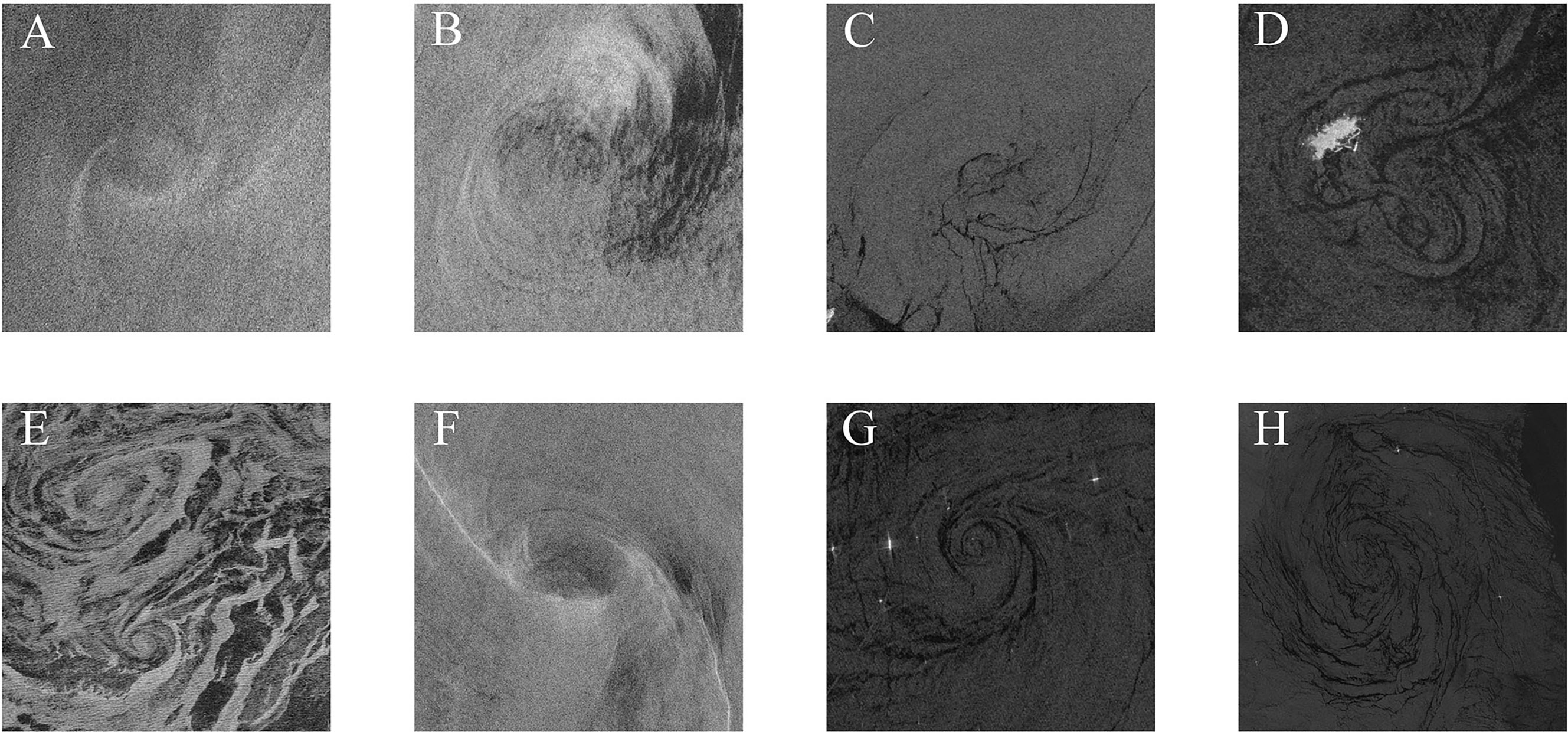
Figure 1 Oceanic eddies in Sentinel-1 SAR images. (A-D) Anticyclonic eddies. (E-H) Cyclonic eddies.

The study of mesoscale or submesoscale oceanic eddies based on SAR images can be traced back to 2000 (Munk et al., 2000). However, numerous studies confirm the location, diameter, vorticity, and manifestation types of oceanic eddies by visually inspecting at full resolution, and further analyzing them from the oceanographic point of view (Munk et al., 2000; Kozlov et al., 2019; Stuhlmacher and Gade, 2020; Ji et al., 2021). Apart from manual interpretation, the algorithms of eddy detection are mainly divided into image transformation-based (Karimova, 2017), handcrafted feature-based (Chen et al., 2019; Du et al., 2019a), and machine learning-based (Du et al., 2019a). Karimova (Karimova, 2017) proposed an algorithm incorporating various image transformations to detect black eddies, which are reflected by surfactant films. Du et al. (Du et al., 2019a) designed an adaptive weighted multi-feature fusion algorithm for automatic mesoscale ocean eddies recognition. The recognition method can meet the requirements of marine complex and changeable environment, with the optimal accuracy reaching 93.42%. In recent years, deep learning, as an essential technical tool in the field of image recognition, has also been widely used in the remote sensing field and has yielded fruitful achievements (Ma et al., 2019; Cheng et al., 2020). Convolutional neural networks (CNNs) with some plug-and-play modules have been reported for detecting oceanic eddies (Du et al., 2019b; Yan et al., 2019; Zhang et al., 2020). Du et al. (Du et al., 2019b) proposed a workflow combining machine learning and deep learning to identify eddies automatically. The principal component analysis (PCA) convolution and spatial pyramid pooling (SPP) are embedded to learn object features and fuse multi-scale information. Finally, a linear classifier distinguishes the oceanic eddies and other phenomena. Yan et al. (Yan et al., 2019) utilized the encoder-decoder architecture to classify five types of oceanic phenomena (including eddies) based on the augmented Sentinel-1 dataset. The architecture contains the backbone ResNet-50 network, followed by the Atrous Spatial Pyramid Pooling (ASPP). Zhang et al. (Zhang et al., 2020) set the Canny edge detection result and the original image as input to mask region-based convolutional networks, further improving the detection accuracy of oceanic eddies.

Although the methods mentioned above have powerful performance in oceanic eddies detection or segmentation tasks, they still have significant limitations. Previous research used powerful deep learning models to implement image-level classification, while more valuable attributes of oceanic eddies were ignored, such as location and diameter. On the other hand, the benchmarking datasets of SAR oceanic eddies are scarce, but the deep learning model requires massive amounts of labeled data resources. Under this background, this study explores the ability of object detection networks framework in eddy detection for SAR images. Meanwhile, a robust and practice network framework called CEA-Net is proposed to effectively detect submesoscale eddies in Sentinel-1 interferometric wide swath (IW) data. The max pooling, dilated convolution, and attention mechanisms are incorporated into CEA-Net to extract features of oceanic eddies. The max pooling and dilated convolution with different coefficients enable the networkto focus on global and multi-scale contextual information. The spatial and channel attention mechanisms are reasonably used to collect favorable information and enhance feature representation. Compared to other plug-and-play modules, these two mechanismshave lower computational complexity and, thus, benefit submesoscale oceanic eddies detection from SAR images. The main contributions and innovations of our research are summarized below.

1. To improve the feature representation capability, the one-stage network called CEA-Net is built for submesoscale eddies detection from Sentinel-1 SAR images. The max pooling and multi-parallel dilated convolutions are embedded behind the backbone network to fuse multi-scale contextual information. The edge information fusion module is assembled to extract available edge information by integrating channel and spatial attention.

2. A multi-scale eddy detection strategy is proposed for complex and large-scale panoramic SAR remote sensing scenes. The strategy can filter out incorrect anchor boxes by calculating the IoU matrix and designing the corresponding constraint rules. It improves the application ability of the deep learning model in real-world scenarios.

3. A novel SAR eddies detection dataset, SAR-Eddy 2019 Dataset, is constructed to facilitate the submesoscale oceanic eddies detection study further. The eddy dataset can be used as a benchmark resource for developing state-of-the-art (SOTA) models for submesoscale oceanic eddies detection.

The dataset and code in this paper will be updated to GitHub: https://github.com/LinghuiXia/SAR-Eddy-Detection. The rest of this article is organized as follows. In Preliminaries, we describe the problem formulation and the details of the SAR-Eddy 2019 dataset used in this research. The proposed CEA-Net and multi-scale eddy detection strategy are introduced in methodology. Results demonstrates the effectiveness of CEA-Net, including comparison with other SOTA methods, ablation study, and the complexity and speed analysis of networks. Finally, Conclusions condenses our research.

2. Preliminaries

2.1. Problem formulations

The task of our problem is to find all submesoscale oceanic eddies in the image and determine their types and location. The object detection model that incorporates detection and classification can meet this need. Inspired by the YOLO series (Redmon et al., 2016; Redmon and Farhadi, 2017; Redmon and Farhadi, 2018; Bochkovskiy et al., 2020; Ge et al., 2021), the one-stage detector will be used in this research, which formulates the detection problem as a regression problem. To better understand this question, the process is described using mathematical language.

Let X∈ℝ^C×H×W as an input SAR image of height H, width W, and channel C. Then, the image X is divided into a S×S grid, and each grid cell is responsible for predicting the corresponding area. By feature extraction and head prediction, each grid cell will be associated with a feature vector to estimate the center coordinates, overall dimensions, and class probability of the object detected. The feature vector can be expressed as:

$\begin{array}{ll}Y=B\times \left\{confidence,\left(x,y\right),h,w,class\_probability\right\}& (1)\end{array}$

where B represents the number of prior anchor boxes, confidence is a signal to judge whether the prior anchor box contains objects, (x,y),h,w are the center coordinates, height, and width of prior anchor boxes predicted, respectively, and class_probability is a vector of length n, representing the probability that the prior anchor box belongs to each category. The class_probability should satisfy the following constraint condition:

$\begin{array}{ll}\{\begin{array}{l}class\_probability=\left\{c_1,c_2,\dots ,c_n\right\}\hfill \\ s.t.\sum _{i=0}^n{c}_i=1\hfill \end{array}& (2)\end{array}$

Thus, these variables that can represent the accuracy of detection results should be optimized by the loss function. The loss function of object detection is defined by the following equation:

$\begin{array}{ll}Los{s}_{total}=Los{s}_{shape}+Los{s}_{confidence}+Los{s}_{class}& (3)\end{array}$

Where Loss_shape, Loss_confidence, Loss_class denote the shape loss, confidence loss, and classification loss of the predicted anchor box, respectively. Their basic components are binary cross-entropy (BCE) loss and mean squared error (MSE) loss. Specific descriptions of the loss function can be found in the published literature (Redmon and Farhadi, 2018; Bochkovskiy et al., 2020; Ge et al., 2021).

2.2. SAR-Eddy 2019 dataset

The SAR-Eddy 2019 dataset is derived from Sentinel-1 images gathered between January and December 2019 (by ASF Data Search: https://search.asf.alaska.edu). The Sentinel-1 is equipped with a C-band (5.405 GHz) synthetic aperture radar, which acquires images regardless of the weather. It also is the only satellite in orbit with publicly accessible data, providing data support for big data research. In this article, the Sentinel-1 Interferometric Wide (IW) Swath GRD Product (20 m × 22 m spatial resolution, 10 m pixel spacing, and 250 km bandwidth) is selected as raw data. The polarization modes of IW data are VH and VV. According to previous research (Du et al., 2019a; Du et al., 2019b; Yan et al., 2019; Zhang et al., 2020), the VV polarization image is used for oceanic eddies recognition. Then, some indispensable preprocessing is performed on raw data, such as the application of orbit file, noise removal, terrain correction, and dB transformation. In the initial data collection stage, the China Sea was the primary study area, which mainly includes the Bohai Sea, Yellow Sea, East China Sea, South China Sea, and Taiwan Strait. We note, however, that the number of anticyclonic eddies interpreted from SAR images is much less than the number of cyclonic eddies. The possible reasons for this phenomenon have been explained in the published research (Xu et al., 2015). Thus, the Japan Sea, Okhotsk Sea, Tokyo Bay, and other waters are included in the research area for increasing the number of anticyclonic eddies. The final study area is situated between 2.82°N and 55.59°N, 102.87°E and 162.74°E (Figure 2A).

FIGURE 2

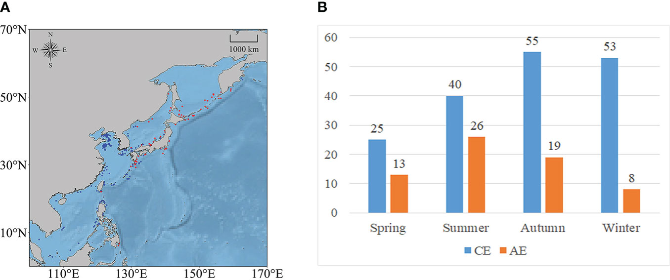
Figure 2 (A) Geographic distribution and (B) seasonal statistics of anticyclonic eddies (red dots) and cyclonic eddies (blue dots) in the SAR-Eddy 2019 dataset.

In this study, 239 SAR images containing eddies were obtained by manual interpretation. Each image contains at least one oceanic eddy. The minimum circumscribed rectangle of the eddy is the ground truth bounding box. Figure 2B counts the number of cyclonic and anticyclonic in the different seasons. Additionally, the radius of screened oceanic eddies ranges from about 2 km to 65 km. Consequently, these eddies differ significantly not only in season, location, scale, radius, and vorticity, butalso in visual characteristics, space features, and texture information (Figure 1). According to the ratio of 7:2:1, the datasets were divided into the training set, validation set and test set, which respectively contained 172 images, 43 images, and 24 images. Meanwhile, 11 large-scale (>50,000 km²) images were used to validate the effectiveness of multi-scale eddy detection strategy. The generalization and robustness of the object detection network are limited by the diversity and volume of the dataset. Because of the above reason, the data augmentation strategy was adopted to expand the original dataset. Scaling with random coefficient, flipping, adding noise, and transforming in color gamut are taken on the original eddy images and their corresponding annotations.

3. Methodology

3.1. Overview of the proposed model framework

Inspired by the traditional one-stage object detection networks, the CEA-Net, which is a context and edge information association network, is proposed for submesoscale eddy detection tasks from Sentinel-1 image. The overview of the network framework is shown in Figure 3. The proposed network takes Darknet-53, which incorporates the residual structure, as a backbone to extract multilevel features. Feature maps of different levels or sizes {52×52,26×26,13×13} areselected from the hierarchical feature maps to detect multi-scale submesoscale oceanic eddies. Among, the low-level features include information on the edges and contours of the eddies. In contrast, the high-level features are shown as oceanic eddy-like targets visible to human eyes. To further enhance the contextual representation of the network for oceanic eddies, the feature spatial pyramid module is plugged into the backbone network. In addition, based on the attention mechanism, the information fusion module that can associate the contextual information and edge information is designed to ensure the integrity of detection results. Ultimately, the proposed multi-scale eddy detection strategy is used to promote the application of the model on large-scale remote sensing images. These parts will be elaborated in following subsection.

FIGURE 3

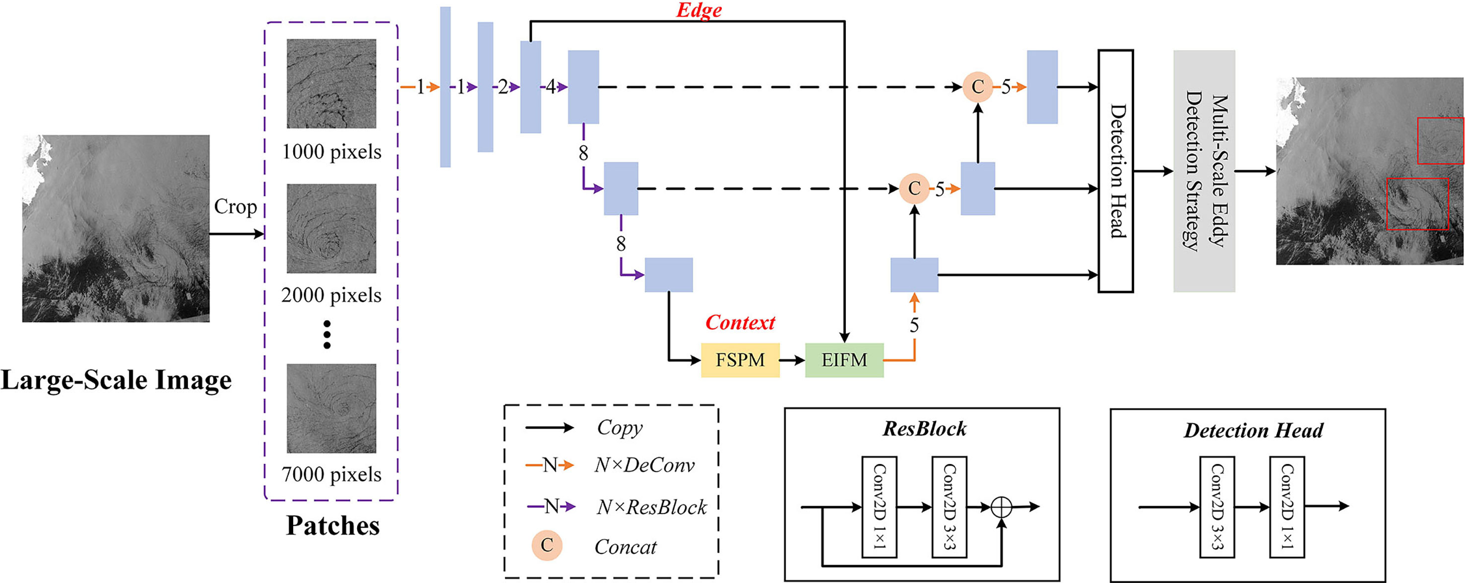
Figure 3 The overall flowchart of the proposed algorithm. A large-scale SAR image is first cropped into patches and then orderly fed to CEA-Net to predict preliminary results. The multi-scale eddy detection strategy reasonably filters the preliminary boxes to obtain submesoscale eddies detection results accurately.

3.2. Feature spatial pyramid module

Appending additional parallel architecture after the backbone network is one of the most effective ways to extract multi-scale contextual information. Currently, many representative works have been proposed and are widely used. The spatial pyramid pooling (SPP) from SPPNet (He et al., 2015), the pyramid pooling module (PPM) from PSPNet (Zhao et al., 2017), and the atrous spatial pyramid pooling (ASPP) from DeepLab (Chen et al., 2017) are state-of-the-art parallel architectures for extracting the enhanced context information further. SPP module solves the problem that CNN needs to fix the dimensions of the input image, which leads to loss of accuracy, by carrying out max pooling on different scale grids. PPM collects global information at different scales by the average pooling with different kernels. ASPP uses atrous convolution with different rates to capture the context feature of the image at multi-scale without loss of resolution.

Inspired by the above methods, the feature spatial pyramid module (FSPM) was designed to obtain enhanced contextual information by merging max pooling and multiple dilated convolutions with different receptive fields. The FSPM consists of five parallel branches. The residual structure is added to maintain original features in the first branch. Then, the next branch adopts global max pooling to generate global feature information. The following three branches applied three dilated convolutions with rates of 1, 2, and 4 for producing features with greater receptive fields. In the end, the output features of the individual branches are further integrated by convolutional blocks as the output of FSPM. The detailed structure of FSPM and convolution block are shown in Figure 4. The parallel pyramid architecture extracts different scale information, while the concatenate operation allows for the better integration of global and local semantic context information for eddy detection.

FIGURE 4

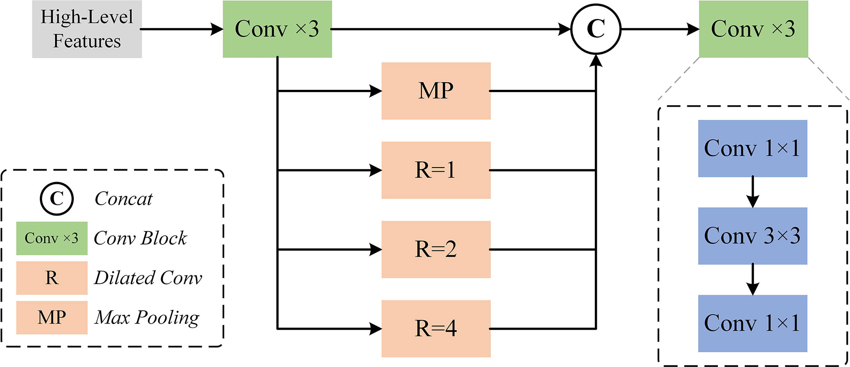
Figure 4 The framework of feature spatial pyramid module (FSPM).

3.3. Edge information fusion module

With the aim to enhance the ability of the network to detect ocean eddy integrity, EIFM is proposed. The EIFM is used to selectively collect edge information from low-level features and contextual information from high-level features, and then associate the filtered information to form high-level features that contain edge information. The channel attention mechanism and spatial attention mechanism are the basic components of the EIFM.

3.3.1. Channel attention mechanism

The channel attention produces a channel attention map by exploiting the interchannel relationship of features (Woo et al., 2018). As shown in Figure 5A, assuming an input feature map F=[f₁,f₂,…,f_C]∈ℝ^C×H×W as input to the channel attention module. First, the global average pooling and global max pooling are used to aggregate the spatial information of the feature map F, generating average-pooled feature and max-pooled feature: $F_{avg}^c,F_{\max }^c\in {ℝ}^{C\times 1\times 1}$. Its cth element is calculated:

FIGURE 5

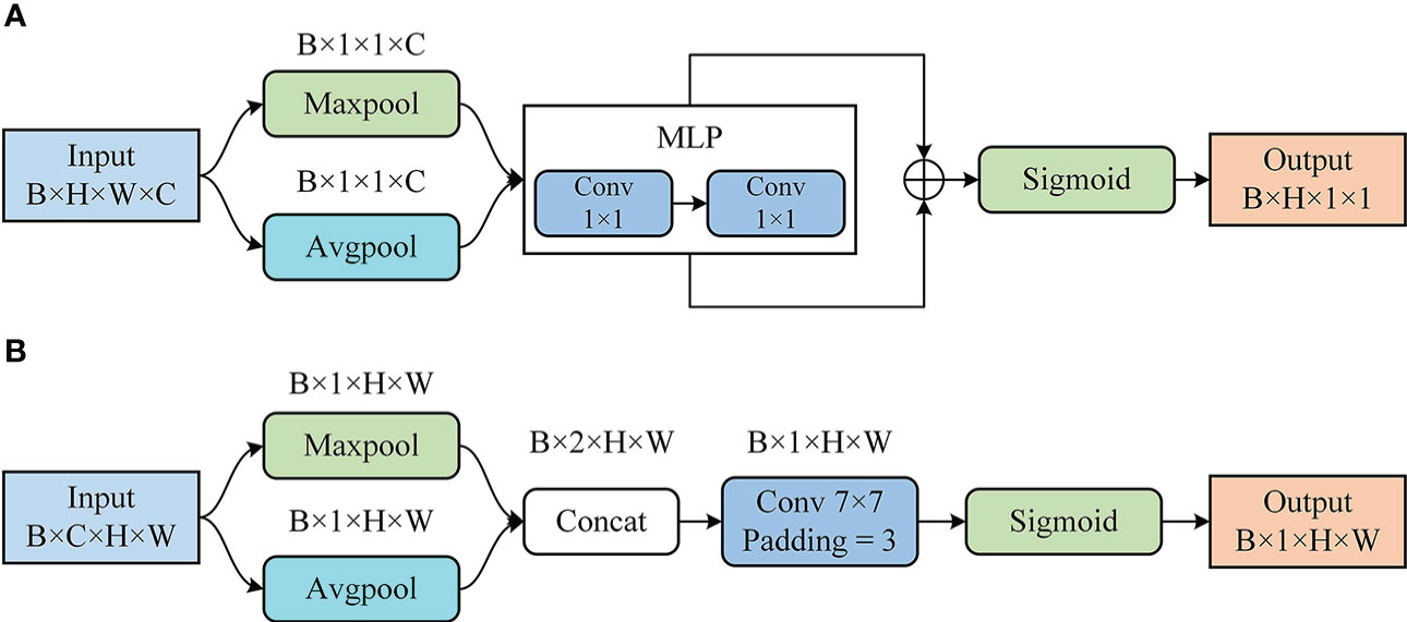
Figure 5 The attention mechanism. (A) Channel attention. (B) Spatial attention.

$\begin{array}{ll}{F}_{avg}^c=\frac{1}{H\times W}\sum _{i=0}^H\sum _{j=0}^W{f}_c\left(i,j\right)& (4)\end{array}$

$\begin{array}{ll}{F}_{max}^c=max\left(f_c\right)& (5)\end{array}$

Subsequently, both features are fed into a shared multi-layer perceptron (MLP) to create feature maps for channel attention, in which the shared MLP is constituted by two fully connected layers. The shared MLP can be formulated as follows:

$\begin{array}{ll}MLP(•)=W_1\left({\delta }_{ReLU}\left(W_0(•)\right)\right)& (6)\end{array}$

Where W₀ and W₁ are the relevant weights of the shared MLP, δ_ReLU(•) denotes the ReLU function.

The output feature vectors after shared MLP are fused by using element-wise summation operation. In the end, the weights for each feature channel are generated by the excitation operation. In brief, the calculation of channel attention is expressed by a mathematical formula as follows:

$\begin{array}{ll}\begin{array}{ll}{M}_c\left(F\right)\hfill & ={\delta }_{sigmoid}\left(MLP\left(AvgPool\left(F\right)\right)\oplus MLP\left(MaxPool\left(F\right)\right)\right)\hfill \\ \hfill & ={\delta }_{sigmoid}\left(W_1\left(W_0\left(F_{avg}^c\right)\right)\oplus W_1\left(W_0\left(F_{max}^c\right)\right)\right)\hfill \end{array}& (7)\end{array}$

Where δ_sigmoid(•) denotes the sigmoid function, ⊕ is the element-wise summation.

3.3.2. Spatial attention mechanism

The structure of spatial attention is illustrated in Figure 5B. As a complement to channel attention, the spatial attention mechanism centers on mining the inter-spatial relationships of feature maps (Woo et al., 2018). The input data are thefeature map, F=[f₁,f₂,…,f_C]∈ℝ^C×H×W , which is the same as the input data in channel attention. First, the global average pooling and global max pooling aggregate the feature information along the channel axis and concatenate them into a combined feature operator: $\left[F_{avg}^c,F_{\max }^c\right]\in {ℝ}^{2\times H\times W}$. And then, a convolution layer and excitation operation are used on the concatenated feature descriptor to generate spatial attention weights M_s(F). The detailed process is as follows:

$\begin{array}{ll}\begin{array}{ll}{M}_s\left(F\right)\hfill & ={\delta }_{sigmoid}\left(Con{v}^{7\times 7}\left(\left[AvgPool\left(F\right);MaxPool\left(F\right)\right]\right)\right)\hfill \\ \hfill & ={\delta }_{sigmoid}\left(Con{v}^{7\times 7}\left(\left[F_{avg}^s;F_{max}^s\right]\right)\right)\hfill \end{array}& (8)\end{array}$

where Conv^7×7(•) is a 2D convolution operation with the kernel size of 7 × 7.

3.3.3. Integration of channel and spatial attention

The EIFM includes channel and spatial attention mechanisms to selectively highlight important information in the spatial and channel domains, respectively. As shown in Figure 6, the spatial and channel attention are linked by parallelism with features at different levels.

FIGURE 6

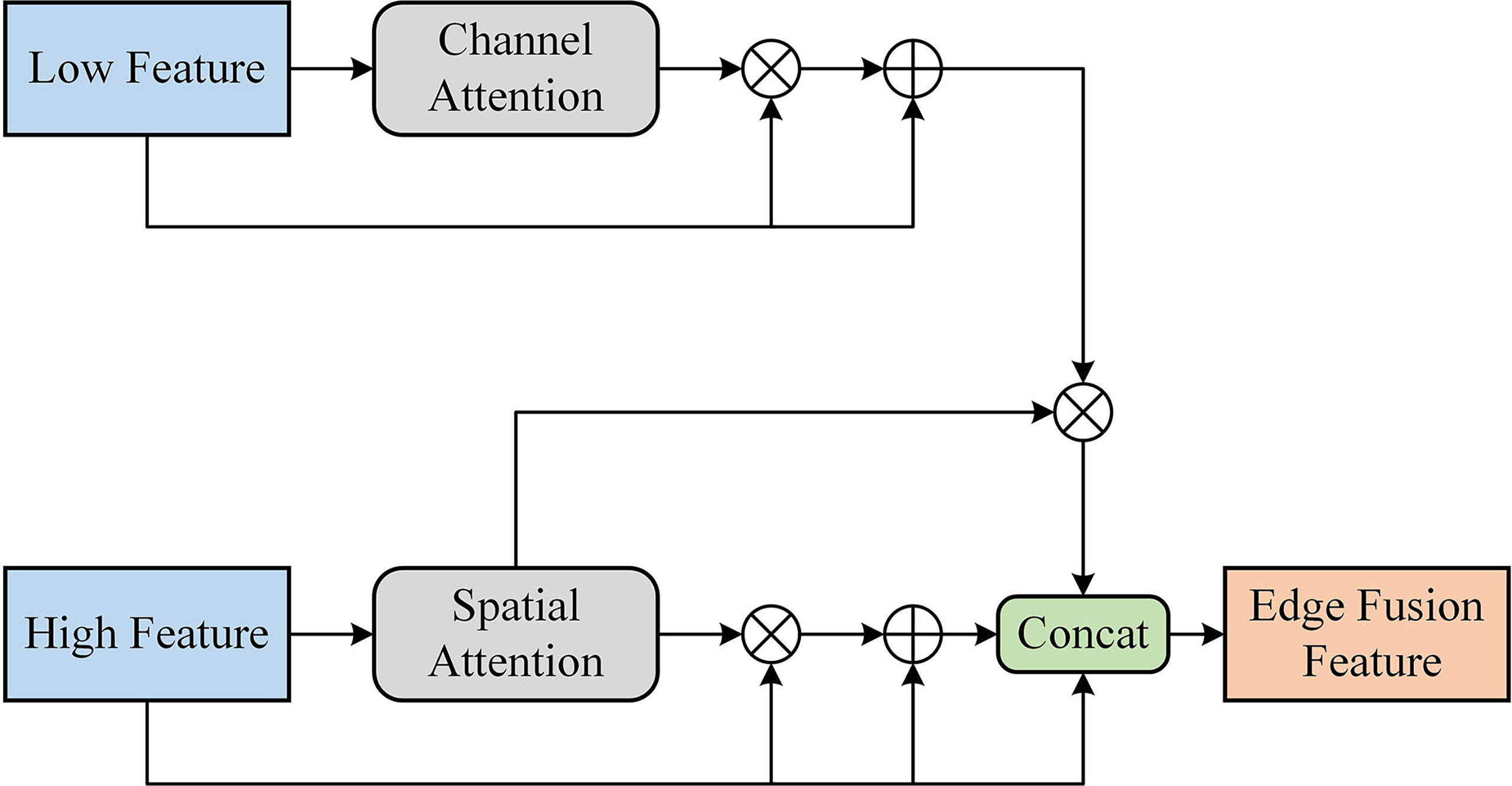
Figure 6 The framework of edge information fusion module (EIFM).

Firstly, the channel attention weights M_c(F) have been used for the low-level feature $F_{low}\in {ℝ}^{C\times \left(\frac{H}{4}\right)\times \left(\frac{W}{4}\right)}$ to make the model more discriminative for each channel. Then, the original low-level feature is introduced to sum with the transformed feature of the weights multiplication. The final edge information is obtained by multiplying the above result and spatial attention weights of the high-level feature. The calculation of the edge information can be summarized as follows:

$\begin{array}{ll}{F}_{edge}=M_s\left(F_{high}\right)\otimes \left(F_{low}\oplus \left(F_{low}\otimes M_c\left(F_{low}\right)\right)\right)& (9)\end{array}$

Where ⊕ and ⊗ denote element-wise summation and multiplication, respectively. The high-level feature $F_{high}\in {ℝ}^{C\times \left(\frac{H}{32}\right)\times \left(\frac{W}{32}\right)}$ is first transformed through the spatial attention weights M_s(F). To preserve the original contextual information, the initial high-level feature is introduced after the feature has been transformed. The formulation of the contextual information is defined as:

$\begin{array}{ll}{F}_{context}=F_{high}\oplus \left(F_{high}\otimes M_s\left(F_{high}\right)\right)& (10)\end{array}$

Finally, the three different levels of features are concatenated, including the high-level feature, contextual information feature, and edge information feature.

$\begin{array}{ll}{F}_{fusion}=\left[F_{high};F_{context};F_{edge}\right]& (11)\end{array}$

This module can selectively fuse edge and contextual information from multilevel features, fully exploiting the edge feature of eddies while suppressing less critical information. It should be emphasized that the EIFM module does not significantly increase network parameters and computational load, but it can prominently improve network performance.

3.4. Multi-scale eddy detection strategy

Considering the practical application of CEA-Net on large-scale remote sensing images, the proposed method was tested on several complete Sentinel-1 interferometric wide swath images. However, different from identifying eddies on data sets, complete remote sensing images cover a wider range and contain ocean eddies of different scales, which is an enormous challenge for applying deep learning models. The multi-scale ocean eddy detection strategy is proposed to solve the above question. The proposed multi-scale eddy detection strategy dealing process is summarized in Algorithm 1.

ALGORITHM 1 MULTI-SCALE EDDY DETECTION STRATEGY METHOD.

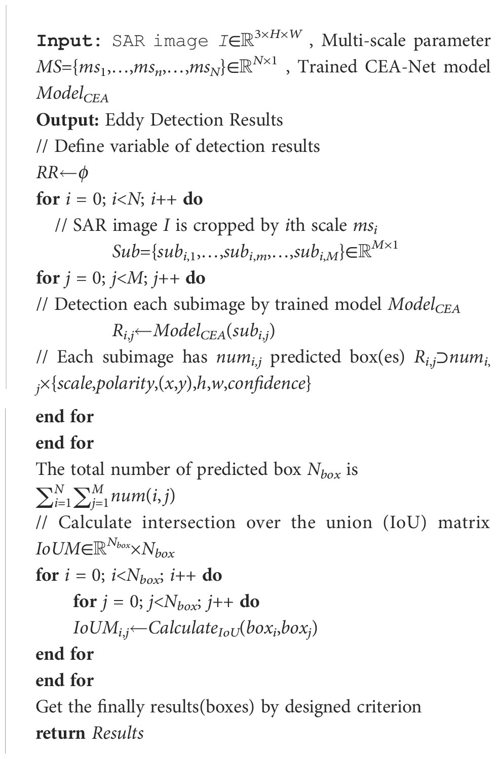
Algorithm 1 Multi-scale eddy detection strategy method..

Firstly, the multi-scale parameter MS = {ms₁,…, ms_n,…, ms_N} with N scales was predefined for a full Sentinel-1 image I. For scale ms₁, the image I is cropped as a series of sub-images with side length ms₁, after which all cropped subimages are summarized according to different scales and then detected by CEA-Net. It is worth noting that the detection result is represented by anchor box. The detection results of subimage sets Sub={sub_i,1,…,sub_i,m,…,sub_i,M}∈ℝ^M×1 on ith scales are represented as follows:

$\begin{array}{ll}\{\begin{array}{l}{R}_{i,j}=\text{\hspace{0.17em}Model}{}_{CEA}\left(\text{\hspace{0.17em}sub}{}_{i,j}\right)\hfill \\ R_{i,j}\supset \text{\hspace{0.17em}num}{}_{i,j}\times \left(\text{\hspace{0.17em}scale},\text{\hspace{0.17em}polarity\hspace{0.17em}},\left(x,y\right),h,w,\text{\hspace{0.17em}confidence\hspace{0.17em}}\right)\hfill \end{array}& (12)\end{array}$

where sub_i,j represents the jth subimage in the ith scale; Model_CEA is the trained CEA-Net; R_i,j is the predicted information of sub_i,j; num_i,j denotes the number of box predicted by CEA-Net in sub_i,j; and scale, polarity, (x, y), h, w, confidence represent the scale information, eddy polarity, center coordinates, height, width, and confidence of each anchor box predicted, respectively.

Therefore, the total num of prior anchor boxes predicted can be calculated as follows:

$\begin{array}{ll}{N}_{box}=\sum _{i=1}^N\sum _{j=1}^M\text{num }(i,j)& (13)\end{array}$

Then, for each detected result, one intersection over the union (IoU) matrix IoUM∈ℝ^Nbox×Nbox will be calculated between each detected result and other results. The IoU is the overlap ratio between the detected box (DT) and the corresponding ground truth box (GT). In this experiment, each detection result is used successively as GT to calculate IoU with other boxes. The other boxes here are seen as DT. The IoU can be calculated by the following equation (14):

$\begin{array}{ll}IoU=\frac{S_{DT}{\cap }^{}{S}_{GT}}{S_{DT}{\cup }^{}{S}_{GT}}& (14)\end{array}$

where IoU constitutes the IoU matrix IoUM, S represents the pixel areas of the anchor box, S_DT∩S_GT is the intersection area of DT and GT, and S_DT∪S_GT denotes their union area.

In the following, the finally detected results must conform to the following criteria: (1) the threshold value of IoU is given as 0.65; (2) the same eddy must be detected by detection boxes of at least two different scales; (3) the detection box with the maximum confidence is the final result of the same eddy.

After the above rules, the final detection results of ocean eddy are obtained on large-scale remote sensing images.

4. Experiments

In this section, the effectiveness of the CEA-Net network is evaluated on the SAR-Eddy 2019 dataset from Sentinel-1. First, the CEA-Net is compared with prevalent and progressive object detection methods to prominent its superiority. Beyond comparison, weconduct experiments on large-scale Sentinel-1 IW images to further demonstrate the practical application ability of CEA-Net and the effectiveness of the multi-scale eddy detection strategy. Finally, the MODIS chlorophyll-a and sea surface temperatures (SST) are employed to verify the correctness of detection results.

4.1. Implementation details

In this paper, all models were implemented on the Pytorch 1.9.0 of the deep learning framework. These experiments were performed on an NVIDIA GeForce RTX 2080 GPU with CUDA 11.3. In order to accelerate the model convergence and reduce memory consumption, the Adam optimizer is selected to learn the parameters of all models automatically. The initial value of the learning rate is pre-set to 0.0001 and is automatically decayed by a factor of 0.92 in each epoch. All networks have been trained for 100 epochs. The batch sizes of the first 50 epochs and the last 50 epochs were fixed to 8 and 4, respectively. The loss function of our model inherits the loss function of the YOLO series, which mainly includes shape loss, confidence loss, and classification loss of the predicted box.

4.2. Evaluation metrics

To evaluate the detection performance of the CEA-Net, some evaluation metrics were used: precision, recall, F1-score, average precision (AP), and mean average precision (mAP). The precision and recall are defined successively using equations (15) and (16):

$\begin{array}{ll}Precision=\frac{TP}{TP+FP}& (15)\end{array}$

$\begin{array}{ll}Recall=\frac{TP}{TP+FN}& (16)\end{array}$

where TP, FP, and FN denote the number of true positive, true negative, and false positive anchor boxes, respectively. In our experiment, the TP means the number of boxes whose IoU is greater than 0.5 between the predicted and ground truth box.

Besides, F1-score measures the comprehensive performance of the network, which can be calculated based on precision and recall.

$\begin{array}{ll}F1-score=\frac{2\times Precision\times Recall}{Precision+Recall}& (17)\end{array}$

The precision and recall of a specific category are used to draw curves in the 2-D coordinate system, and the area under the curve is AP of this category.

$\begin{array}{ll}AP=\underset{0}{\overset{1}{\int }}P\left(R\right)dR& (18)\end{array}$

According to equation (19), mAP can be furnished, which represents the average of all categories of AP:

$\begin{array}{ll}mAP=\frac{{\sum }_{i=1}^{n}A{P}_i}{n}& (19)\end{array}$

The AP and mAP are commonly considered indicators of model quality. Generally speaking, the two indicators and model quality are positively correlated.

4.3. Result and analysis

In this section, the CEA-Net was compared with SSD (Liu et al., 2016), Faster RCNN (Ren et al., 2015), Retinanet (Lin et al., 2017), YOLOv3 (Redmon and Farhadi, 2018), YOLOv4 (Bochkovskiy et al., 2020), and YOLOx (Ge et al., 2021) in the specific study area of the SAR-Eddy 2019 Dataset. Meanwhile, the detection performances of different networks were also compared from both qualitative and quantitative analyses.

Figure 7 shows the visualization comparison of the eddy detection result by different networks in five representative SAR eddy images. From these complicated images, it can be observed that the conspicuous obstacle of eddy detection is the clutter, intense speckle effect, and easily-confused sea surface phenomena (oil film and ship tracks). The eddy scenarios are provided for five different sea states. The eddy images in the first column have a low backscattering coefficient as a whole, while the second column images are opposite distribution. The third column images illustrate the performance of different networks under oceanic eddies, where the seawater is mixed with large amounts of sea ice. Unlike other eddies with continuous wake, the eddies of the fourth and fifth column images are not visually complete.

FIGURE 7

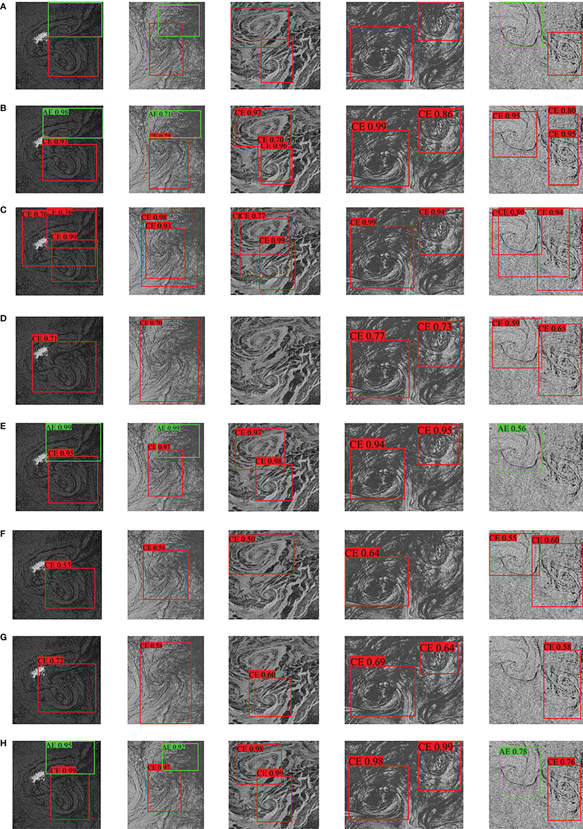
Figure 7 Visualization comparison results of different networks. (A) Ground truths. (B-H) Results of SSD, Faster RCNN, Retinanet, YOLOv3, YOLOv4, YOLOx, and CEA-Net. The confidence score of the displayed boxes is all greater than 0.5.

It is worth mentioning that the prediction boxes of cyclone eddies (CEs) and anticyclone eddies (AEs) are marked with red and green, respectively. After prediction by different networks, and comparative observation of the visualization results, it is found that the detected results of the CEA-Net are closer to the ground truth. Compared with other methods, the results of Retinanet, YOLOv3, YOLOv4, and YOLOx have missed detections, such as the first, third and last column. Meanwhile, according to the experimental results in the second column, these models cannot separate multiple symbiotic eddies effectively. The false positive result was presented in the third column from SSD. Although YOLOv3 can correctly identify most eddies compared with other detection networks, the predicted anchor boxes of YOLOv3 have a poor ability to describe the range of oceanic eddies compared to CEA-Net. It can be seen that, in the first column, the predicted anchor box of CEA-Net is closer to the edge of eddies because EIFM selectively takes into consideration the edge information. Additionally, the results detected by CEA-Net are more consistent with the ground truth. This result indicates that CEA-Net can effectively obtain enhanced contextual information and further suppress noise. Therefore, according to the above discussion, the proposed CEA-Net has good robustness and distinct advantages in terms of visuals.

To further validate our proposed method, the five widely evaluation metrics are used for quantitative analysis. The highest value of indicators is marked in bold. Table 1 shows the precision, recall, and F1-score for our proposed CEA-Net and other mainstream object detection methods. The quantitative metrics from Table 1 show that the CEA-Net has the highest recall and lowest precision standard deviation. Table 2 compares seven SOTA networks of AP and mAPon the eddy dataset, further indicating that our method surpasses other comparison methods. There are significant differences in accuracy between the two-stage (SSD) and single-stage (YOLO) algorithms from Tables 1 and 2. Therefore, the single-stage algorithm is more suitable for unique elliptic or banded objects. From these tables, our CEA-Net achieves the best precision, recall, and F1-score AP for anticyclonic, reaching 85.7%, 85.71%, 85.71%, and 92.76%, respectively. However, cyclonic quantification results do not have the same excellent performance as anticyclones. This situation is caused by the sample imbalance of the SAR-Eddy 2019 dataset. Except these, our CEA-Net achieves 85.47% mAP for oceanic detection task, which is significantly better than other methods, representing improvements of 9.38%, 12.25%, 5.2%, 5.05%, 2.36%, and 3.21% over SSD, Faster RCNN, Retinanet, YOLOv3, v4, and x. These improvements may be primarily due to the fact that, by simultaneously considering global contextual information and preferred edge information, the eddy polarity can be well captured during the category prediction stage. Through the above quantitative evaluation and qualitative analysis, the proposed method of CEA-Net has an outstanding advantage over the current mainstream object detection networks.

TABLE 1

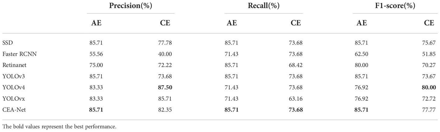
Table 1 Comparison with the different networks in precision, recall, and F1-score.

TABLE 2

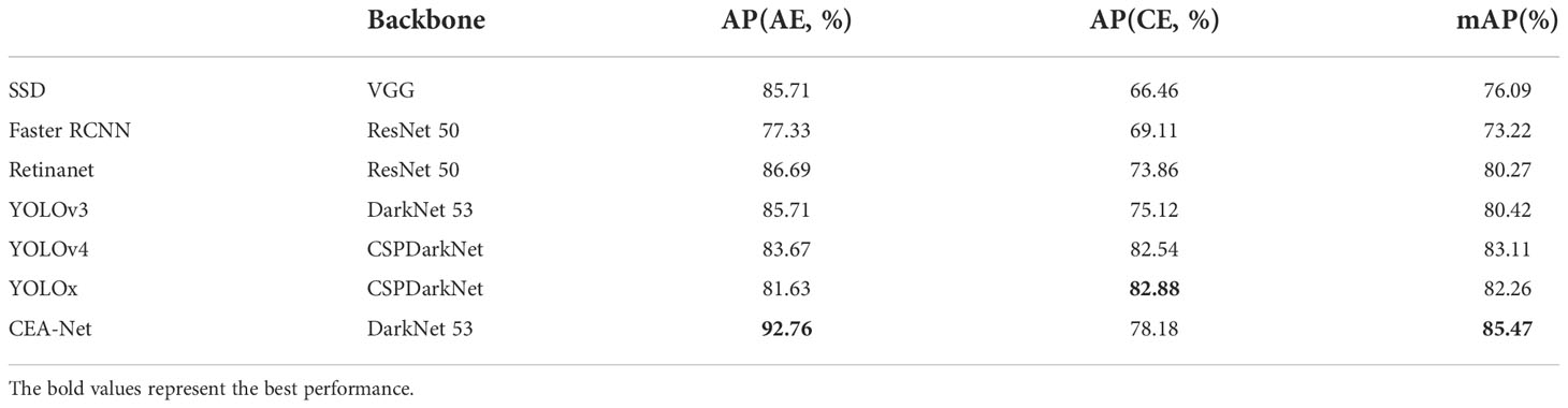
Table 2 Comparison with the different networks in AP and mAP.

To further demonstrate how the CEA-Net works in SAR-Eddy 2019 Dataset, we visualize some feature maps at different positions of the proposed CEA-Net by Grad-CAM (Selvaraju et al., 2017) in Figure 8. Clearly, the proposed EIFM can more effectively collect edge information. For example, the feature map output after EIFM in the last column of Figure 8 can accurately capture the wake feature of oceanic eddies. However, the backbone network (DarkNet-53) and FSPM cannot do this because they lost edge information.

FIGURE 8

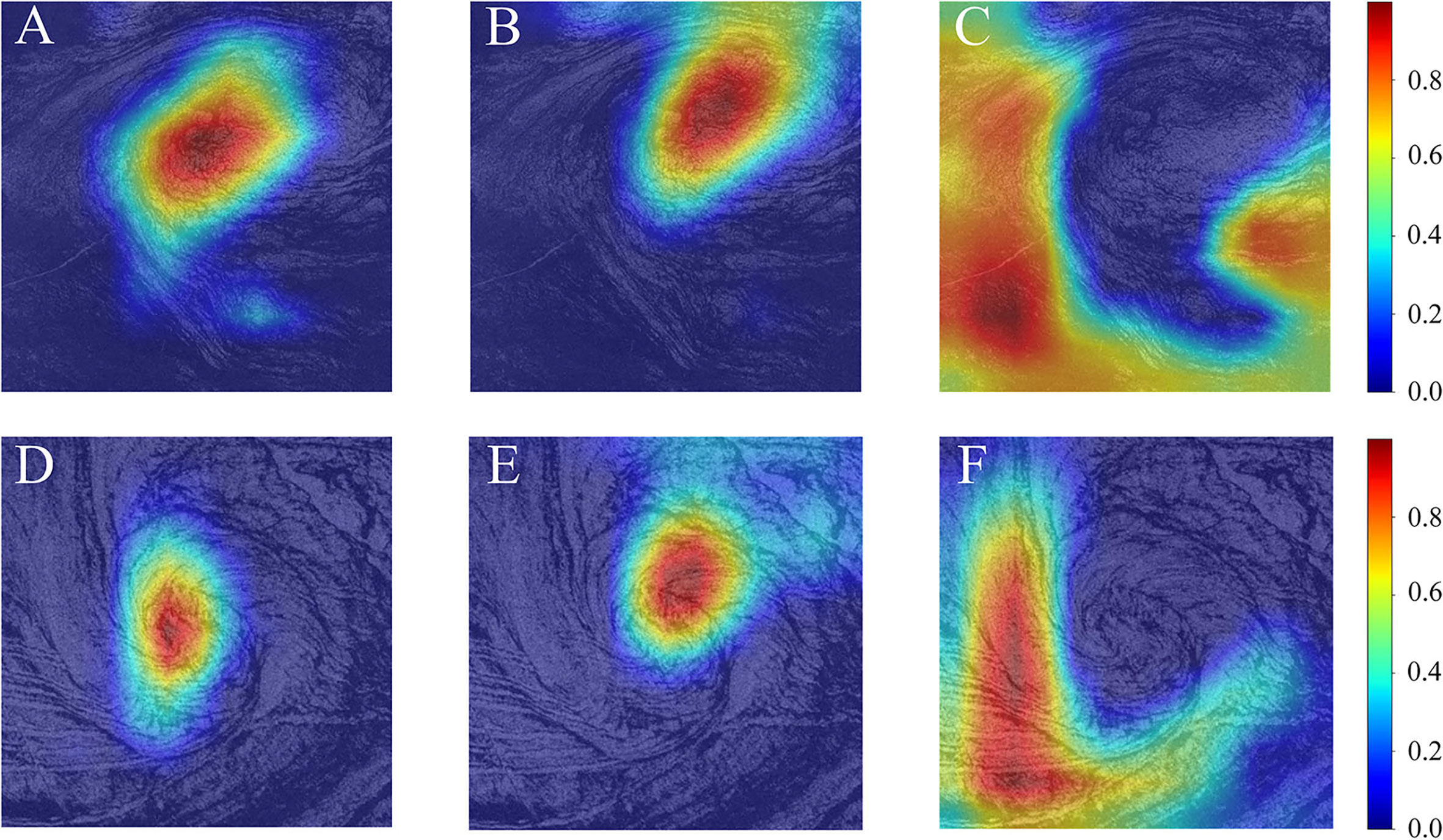
Figure 8 Visualization of selected feature maps at different positions of the proposed CEA-Net. (A, D) After backbone, (B, E) After FSPM, (C, F) After EIFM.

4.4. Detection results on large Sentinel-1 image

The multi-scale eddy detection strategy combined with CEA-Net is applied to large-scale panoramic Sentinel-1 IW SAR images, and the practicality of the eddy detection model was verified. Raw images were preprocessed first by the described Sentinel-1 preprocessing flow in Section 2.2. And then, the linear stretch with 2% is adopted to facilitate the visualization of SAR images. In the following, a series of sub-images by cropping panoramic images were fed into the CEA-Net in batches to achieve the preliminary detection results. Finally, the preliminary detection results can be further filtered based on multi-scale eddy detection strategy, thereby yielding the final precise detection result.

The ability of ocean eddies to transport heat, salinity, tracers, nutrients, and chlorophyll is due to their nonlinear structure. The cyclonic eddy (anticyclonic eddy) causes seawater divergence (convergence) to push the lower (upper) layer of seawater torise (fall) by the geostrophic effect, causing the sea surface to exhibit SST with local minimum (high) values. Meanwhile, the eddy-induced pumping (Falkowski et al., 1991) points out that upwelling within cyclonic eddies enriches the upper ocean withnutrients, significantly increasing chlorophyll-a concentrations in the surface layer. Anticyclonic eddies do the opposite. Thus, the MODIS chlorophyll-a data and SST data are contrasted with the Sentinel-1 image for the same spatio-temporal for verifying the eddies detected.

As an example, the scene name of images selected for display and analysis is S1A_IW_GRDH_1SDV_2019−0805T224332_20190805T224401_028440_0336C6_DCF4, located between 16.33°N and 18.44°N, 105.53°E and 108.33°E. The image was acquired from the South China Sea on August 5, 2019. And it has 24276×29828 pixels covering an area of about 72,116 km². It is worth mentioning that the multi-scale parameter (MS) includes five scales, which are 1000 pixels, 3000 pixels, 5000 pixels, 7000 pixels, and 9000 pixels, respectively, in the experiment. Figures 9A–C show the detection and comparative results. The red dot is the center of the cyclonic eddy. The significant backscatter, high chlorophyll, and cold SST appeared in the corresponding region. This phenomenon thus demonstrates that the eddies detected from SAR are confirmed in the MODIS chlorophyll-a and SST data. Because of the limited spatial resolution of MODIS data and derivative product (chlorophyll-a and SST), the submesoscale oceanic eddies with radial less than 5 km cannot be detected (the left bottom of Figure 9A). Cloud and fog also represent a severe obstacle for optical data to detect eddies. In another set of experiments, an abnormal anticyclonic eddy (Liu et al., 2021) was detected in Sentinel-1 image collected from the Sea of Okhotsk (Sentinel-1 ID: S1A_IW_GRDH_1SDV_20190728T202431_20190728T202500_028322_03333D_0499). The anticyclonic eddy has high chlorophyll and low SST in the corresponding region of MODIS data, which is inconsistent with the chlorophyll and SST distribution of the normal anticyclonic eddy (see Figures 9D–F).

FIGURE 9

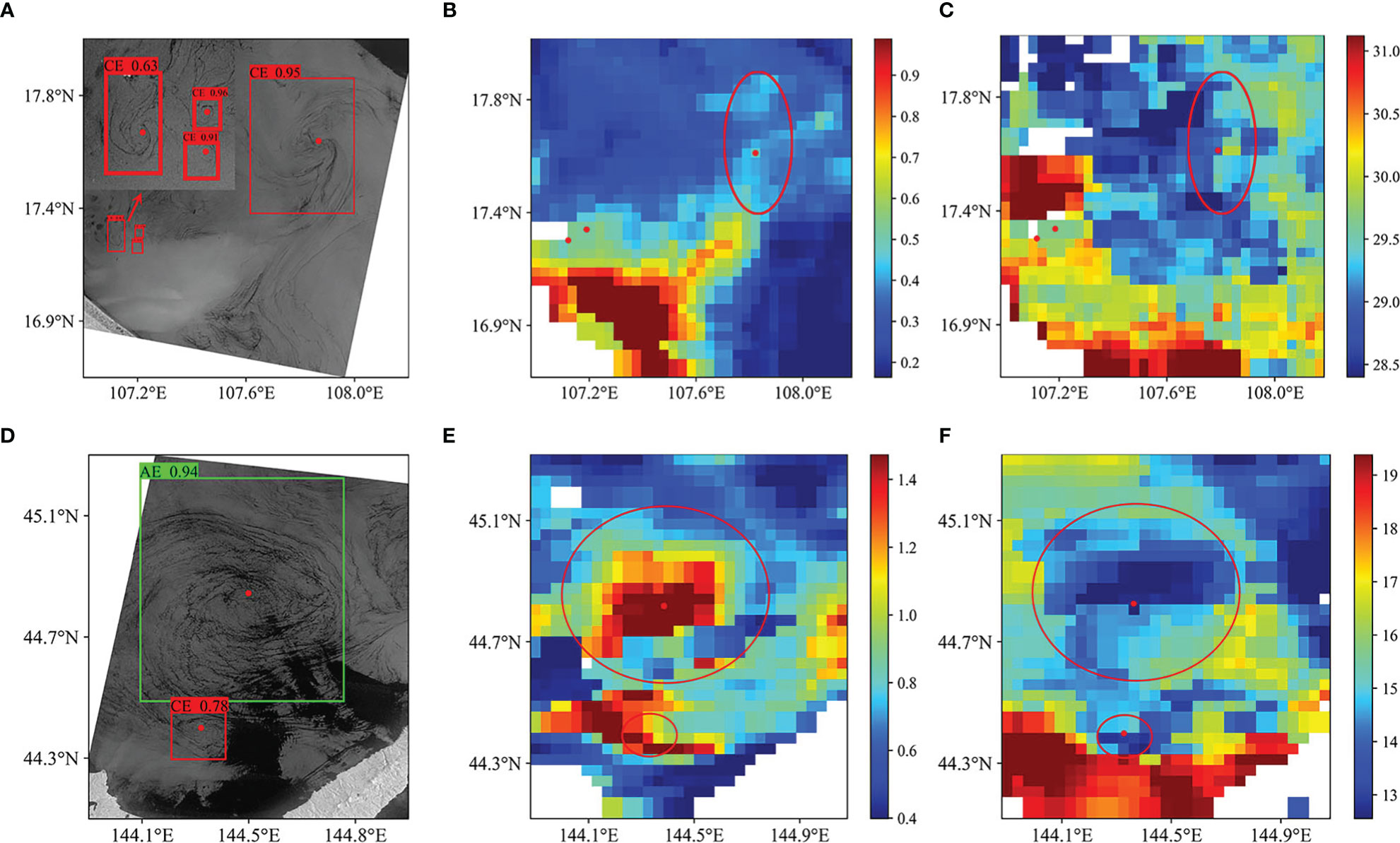
Figure 9 (A, D) Oceanic eddies detected by Sentinel-1 images. (B, E) MODIS chlorophyll-a data. (C, F) MODIS SST data. The dot and outline represent the center and the range of eddies on chlorophyll-a and SST data. Furthermore, the red and green anchor boxes are the cyclone and anticyclone, respectively.

Actually, the identified eddies by merged altimeter data (Tian et al., 2020) were also used to match and compare with the SAR image identification results. However, the matching results are overwhelmingly negative. One of the reasonsis that the interesting area of Sentinel-1 is the coastal waters in the study area, while the altimeter focuses on the deep-sea region. Moreover, the data resolution (about 25 km) of existing altimeters is not suitable to detection submesoscale eddies which horizonal scale are about 10 km, which may result in the negative comparison. Therefore, the detection results of Sentinel-1 SAR data are recommended as a supplement to the altimeter eddies dataset.

The comparison experiment that CEA-Net combined with and without multi-scale eddy detection strategy was designed for better verification the necessity of multi-scale eddy detection strategy. Figure 10 shows the experimental results of thelarge Sentinel-1 images in the study area. It can be seen from Figure 10 that the multi-scale detection strategy proposed in this article improves detection capabilities in capturing small-scale eddies (see Figures 10A, C). If a large-scale image is fed directly into the CEA-Net model, the useful spatial information of small-scale eddies will be lost due to convolution and pooling. Thus, the CEA-Net without multi-scale strategy performs poorly in terms of correctness of small-scale eddies detection (see Figures 10B, D). These illustrate the importance of multi-scale eddy detection strategy for detecting different scale oceanic eddy.

FIGURE 10

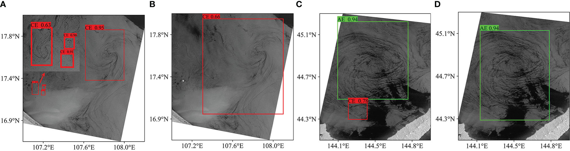
Figure 10 Visualization comparison results of CEA-Net combine with and without multi-scale eddy detection strategy. (A, C) With multi-scale strategy, (B, D) Without multi-scale strategy.

The experimental results indicate not only the effectiveness and practicability of the proposed model and strategy in real scenarios but also embody the superiority of high-resolution SAR data in submesoscale eddy detection.

4.5. Ablation study

In this subsection, the ablation study was designed to remove some modules from the network and thus analyze the contribution of each module, i.e., the feature spatial pyramid module (FSPM), edge information fusion module (EIFM), and the data augmentation strategy (DAAS). The YOLOv3 is selected as the baseline network. Next, the FSPM module and EIFM module are successively introduced into the baseline. Data augmentation is applied online to expand the diversity of data, which does not require an additional training burden. It should be noted that the multi-scale eddy detection strategy was not systematically assessed in the ablation study. The primary function of the strategy is better to apply deep learning models to large remote sensing images, rather than to improve the performance of the models on the dataset.

Table 3 shows the accuracy indicator of ablation experiments, including the AP scores per class and the mAP of each submodel. Without FSMP block, EIFM block, and DAAS strategy, the YOLOv3 obtains the baseline mAP of 77.32%. When the FSPM block was introduced into the baseline model, mAP was improved by 5.28%. Meanwhile, the baseline network with EIFM further improves the mAP and obtains the best AP of CE. With EIFM, the AP of CE was improved by 14.5%, and mAP was improved by 6.23%, indicating that the selective association of edge and contextual features can effectively improve the detection precision of the network. The DAAS enhances the richness of train samples, improves robustness and generalization of the network, and thus improves the prediction effect in the test stage. As can be seen from the metrics in the last row of Table 3, the union of multi-modules furthest optimizes the detection capability of the baseline network. The AP of AE and CE are 92.76% and 78.18%, corresponding to the increase of 7.05% and 9.25%, respectively. In addition, mAP also improved significantly, reaching 85.47%. With the proposed two modules of feature enhancement, the representative eddy information can be well characterized, and the CEA-Net is thus promoted to focus on the object area in the multilevel feature maps.

TABLE 3

Table 3 Ablation study on SAR-Eddy 2019 dataset.

4.6. Complexity and speed analysis

Apart from the accuracy of object detection, runtime efficiency and memory consumption are extremely important for applying the model. Thus, this part summarizes and analyses the number of parameters and inference speed of the proposed CEA-Net, SOTA, and ablation models. Table 4 shows the most SOTA models. Considering the excellent detection performance of the model, the reasoning efficiency and memory consumption are acceptable.

TABLE 4

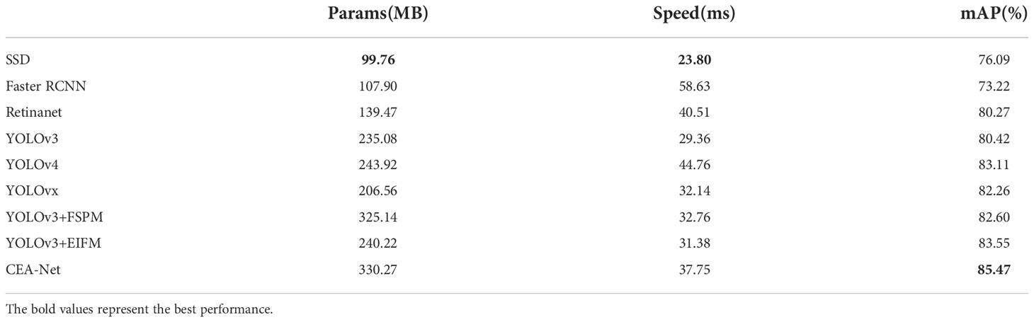
Table 4 Comparison of speed and complexity with other networks.

5. Conclusion

In this paper, an effective and robust model, namely CEA-Net, for submesoscale oceanic eddies detection from SAR images. The CEA-Net integrates both contextual and edge information of submesoscale eddy into the backbone network. It can provide a solution to the difficulties of identifying submesoscale oceanic eddies in fine-resolution SAR imagery as well as the inadequacy of scene-level edge features. A new oceanic eddy dataset, SAR-Eddy 2019 dataset, is established for evaluating the proposed method. The detection results demonstrate the superiority of our proposed CEA-Net in terms of quantitative assessment and visual performance. The multi-scale eddy detection strategy provides a bridge for the application of CEA-Net in large-scale Sentinel-1 images. These results in this research provide some insights for future work. Lightweight and class-imbalance issues will be addressed. Besides, the expansion of the submesoscale oceanic eddies dataset is also on our schedule.

Data availability statement

The original contributions presented in the study are included in the article/supplementary material. Further inquiries can be directed to the corresponding author.

Author contributions

LX performed methodology, software, validation, data curation, visualization, and writing of the original draft. GC contributed to conceptualization, investigation, writing review and editing, and supervision. LG performed the model framework construction. BH performed validation and investigation. XC performed validation and review. All authors contributed to the article and approved the submitted version.

Funding

This research was jointly supported by the National Natural Science Foundation of China (No.42276203), the National Natural Science Foundation of China (Grant No. 42030406), the Natural Science Foundation of Shandong Province (No. ZR2021MD001), and the International Research Center of Big Data for Sustainable Development Goals (CBAS2022GSP01).

Acknowledgments

The authors gratefully appreciate ASF Data Search for the open-source data.

Conflict of interest

The authors declare that the research was conducted in the absence of any commercial or financial relationships that could be construed as a potential conflict of interest.

Publisher’s note

All claims expressed in this article are solely those of the authors and do not necessarily represent those of their affiliated organizations, or those of the publisher, the editors and the reviewers. Any product that may be evaluated in this article, or claim that may be made by its manufacturer, is not guaranteed or endorsed by the publisher.

References

Bochkovskiy A., Wang C.-Y., Liao H.-Y. M. (2020). Yolov4: Optimal speed and accuracy of object detection. arXiv preprint arXiv:2004.10934, 1–17. doi: 10.48550/arXiv.2004.10934

CrossRef Full Text | Google Scholar

Chelton D. B., Schlax M. G., Samelson R. M., de Szoeke R. A. (2007). Global observations of large oceanic eddies. Geophys. Res. Lett. 34, 87–101. doi: 10.1029/2007GL030812

CrossRef Full Text | Google Scholar

Chen G., Ezraty R. (1997). Non-tidal aliasing in seasonal sea-level variability and annual rossby waves as observed by satellite altimetry. Annales Geophysicae 15, 1478–1488. doi: 10.1007/s00585-997-1478-z

CrossRef Full Text | Google Scholar

Cheng G., Xie X., Han J., Guo L., Xia G.-S. (2020). Remote sensing image scene classification meets deep learning: Challenges, methods, benchmarks, and opportunities. IEEE J. Selected Topics Appl. Earth Observations Remote Sens. 13, 3735–3756. doi: 10.1109/JSTARS.2020.3005403

CrossRef Full Text | Google Scholar

Chen L.-C., Papandreou G., Kokkinos I., Murphy K., Yuille A. L. (2017). Deeplab: Semantic image segmentation with deep convolutional nets, atrous convolution, and fully connected crfs. IEEE Trans. Pattern Anal. Mach. Intell. 40, 834–848. doi: 10.1109/TPAMI.2017.2699184

PubMed Abstract | CrossRef Full Text | Google Scholar

Chen J., Yang J., Tao R., Yu Z. (2019). “Mesoscale eddy detection and edge structure extraction method in sar image,” in IOP conference series: Earth and environmental science, (Chengdu: PEOPLES R CHINA: IOP Publishing) 237, 032010.

Google Scholar

D’Alimonte D. (2009). Detection of mesoscale eddy-related structures through iso-sst patterns. IEEE Geosci. Remote Sens. Lett. 6, 189–193. doi: 10.1109/LGRS.2008.2009550

CrossRef Full Text | Google Scholar

Dong C., Xu G., Han G., Chen N., He Y., Chen D. (2018). Identification of tidal mixing fronts from high-resolution along-track altimetry data. Remote Sens. Environ. 209, 489–496. doi: 10.1016/j.rse.2018.02.047

CrossRef Full Text | Google Scholar

Du Y., Liu J., Song W., He Q., Huang D. (2019a). Ocean eddy recognition in sar images with adaptive weighted feature fusion. IEEE Access 7, 152023–152033. doi: 10.1109/ACCESS.2019.2946852

CrossRef Full Text | Google Scholar

Du Y., Song W., He Q., Huang D., Liotta A., Su C. (2019b). Deep learning with multi-scale feature fusion in remote sensing for automatic oceanic eddy detection. Inf. Fusion 49, 89–99. doi: 10.1016/j.inffus.2018.09.006

CrossRef Full Text | Google Scholar

Espeseth M. M., Jones C. E., Holt B., Brekke C., Skrunes S. (2020). Oil-spill-response-oriented information products derived from a rapid-repeat time series of sar images. IEEE J. Selected Topics Appl. Earth Observations Remote Sens. 13, 3448–3461. doi: 10.1109/JSTARS.2020.3003686

CrossRef Full Text | Google Scholar

Falkowski P. G., Ziemann D., Kolber Z., Bienfang P. K. (1991). Role of eddy pumping in enhancing primary production in the ocean. Nature 352, 55–58. doi: 10.1038/352055a0

CrossRef Full Text | Google Scholar

Ge Z., Liu S., Wang F., Li Z., Sun J. (2021). Yolox: Exceeding yolo series in 2021. arXiv preprint arXiv:2107.08430, 1–7. doi: 10.48550/arXiv.2107.08430

CrossRef Full Text | Google Scholar

He K., Zhang X., Ren S., Sun J. (2015). Spatial pyramid pooling in deep convolutional networks for visual recognition. IEEE Trans. Pattern Anal. Mach. Intell. 37, 1904–1916. doi: 10.1109/TPAMI.2015.2389824

PubMed Abstract | CrossRef Full Text | Google Scholar

Ji Y., Xu G., Dong C., Yang J., Xia C. (2021). Submesoscale eddies in the east china sea detected from sar images. Acta Oceanologica Sin. 40, 18–26. doi: 10.1007/s13131-021-1714-5

CrossRef Full Text | Google Scholar

Karimova S. (2012). Spiral eddies in the baltic, black and caspian seas as seen by satellite radar data. Adv. Space Res. 50, 1107–1124. doi: 10.1016/j.asr.2011.10.027

CrossRef Full Text | Google Scholar

Karimova S. (2017). “An approach to automated spiral eddy detection in sar images,” in 2017 IEEE international geoscience and remote sensing symposium (IGARSS) (Fort Worth, TX: IEEE) 743–746. doi: 10.1109/IGARSS.2017.8127059

CrossRef Full Text | Google Scholar

Konik M., Bradtke K. (2016). Object-oriented approach to oil spill detection using envisat asar images. ISPRS J. Photogrammetry Remote Sens. 118, 37–52. doi: 10.1016/j.isprsjprs.2016.04.006

CrossRef Full Text | Google Scholar

Kozlov I. E., Artamonova A. V., Manucharyan G. E., Kubryakov A. A. (2019). Eddies in the western arctic ocean from spaceborne sar observations over open ocean and marginal ice zones. J. Geophys. Res.: Oceans 124, 6601–6616. doi: 10.1029/2019JC015113

CrossRef Full Text | Google Scholar

Lee I. K., Shamsoddini A., Li X., Trinder J. C., Li Z. (2016). Extracting hurricane eye morphology from spaceborne sar images using morphological analysis. ISPRS J. Photogrammetry Remote Sens. 117, 115–125. doi: 10.1016/j.isprsjprs.2016.03.020

CrossRef Full Text | Google Scholar

Le Traon P., Nadal F., Ducet N. (1998). An improved mapping method of multisatellite altimeter data. J. Atmospheric Oceanic Technol. 15, 522–534. doi: 10.1175/1520-0426(1998)015<0522:AIMMOM>2.0.CO;2

CrossRef Full Text | Google Scholar

Lin T.-Y., Goyal P., Girshick R., He K., Dollár P. (2017). “Focal loss for dense object detection,” in Proceedings of the IEEE international conference on computer vision (Venice, Italy: IEEE) 2980–2988.

Google Scholar

Liu W., Anguelov D., Erhan D., Szegedy C., Reed S., Fu C.-Y., et al. (2016). “Ssd: Single shot multibox detector,” in European Conference on computer vision (Amsterdam, The Netherlands: Springer) 21–37. doi: 10.1007/978-3-319-46448-0

CrossRef Full Text | Google Scholar

Liu Y., Zheng Q., Li X. (2021). Characteristics of global ocean abnormal mesoscale eddies derived from the fusion of sea surface height and temperature data by deep learning. Geophys. Res. Lett. 48, e2021GL094772. doi: 10.1029/2021GL094772

CrossRef Full Text | Google Scholar

Ma L., Liu Y., Zhang X., Ye Y., Yin G., Johnson B. A. (2019). Deep learning in remote sensing applications: A meta-analysis and review. ISPRS J. Photogrammetry Remote Sens. 152, 166–177. doi: 10.1016/j.isprsjprs.2019.04.015

CrossRef Full Text | Google Scholar

Marcello J., Eugenio F., Estrada-Allis S., Sangrà P. (2015). Segmentation and tracking of anticyclonic eddies during a submarine volcanic eruption using ocean colour imagery. Sensors 15, 8732–8748. doi: 10.3390/s150408732

PubMed Abstract | CrossRef Full Text | Google Scholar

Munk W., Armi L., Fischer K., Zachariasen F. (2000). Spirals on the sea. Proc. R. Soc. London Ser. A: Mathematical Phys. Eng. Sci. 456, 1217–1280. doi: 10.1098/rspa.2000.0560

CrossRef Full Text | Google Scholar

Ni Q., Zhai X., Wilson C., Chen C., Chen D. (2021). Submesoscale eddies in the south china sea. Geophys. Res. Lett. 48, e2020GL091555. doi: 10.1029/2020GL091555

CrossRef Full Text | Google Scholar

Redmon J., Divvala S., Girshick R., Farhadi A. (2016). “You only look once: Unified, real-time object detection,” in Proceedings of the IEEE conference on computer vision and pattern recognition (Las Vegas, NV, USA: IEEE) 779–788.

Google Scholar

Redmon J., Farhadi A. (2017). “Yolo9000: better, faster, stronger,” in Proceedings of the IEEE conference on computer vision and pattern recognition(Honolulu, USA: IEEE) 7263–7271.

Google Scholar

Redmon J., Farhadi A. (2018). Yolov3: An incremental improvement. arXiv preprint arXiv:1804.02767, 1–6. doi: 10.48550/arXiv.1804.02767

CrossRef Full Text | Google Scholar

Ren S., He K., Girshick R., Sun J. (2015). “Faster r-cnn: Towards real-time object detection with region proposal networks,” in Advances in neural information processing systems, vol. 28 . Eds. Cortes C., Lawrence N., Lee D., Sugiyama M., Garnett R. (Montréal, CANADA: Curran Associates, Inc).

Google Scholar

Selvaraju R. R., Cogswell M., Das A., Vedantam R., Parikh D., Batra D. (2017). “Grad-cam: Visual explanations from deep networks via gradient-based localization,” in Proceedings of the IEEE international conference on computer vision (Venice, Italy: IEEE) 618–626.

Google Scholar

Stuhlmacher A., Gade M. (2020). Statistical analyses of eddies in the western mediterranean sea based on synthetic aperture radar imagery. Remote Sens. Environ. 250, 112023. doi: 10.1016/j.rse.2020.112023

CrossRef Full Text | Google Scholar

Taburet G., Sanchez-Roman A., Ballarotta M., Pujol M.-I., Legeais J.-F., Fournier F., et al. (2019). Duacs dt2018: 25 years of reprocessed sea level altimetry products. Ocean Sci. 15, 1207–1224. doi: 10.5194/os-15-1207-2019

CrossRef Full Text | Google Scholar

Tian F., Wu D., Yuan L., Chen G. (2020). Impacts of the efficiencies of identification and tracking algorithms on the statistical properties of global mesoscale eddies using merged altimeter data. Int. J. Remote Sens. 41, 2835–2860. doi: 10.1080/01431161.2019.1694724

CrossRef Full Text | Google Scholar

Woo S., Park J., Lee J.-Y., Kweon I. S. (2018). “Cbam: Convolutional block attention module,” in Proceedings of the European conference on computer vision (ECCV) (Munich, Germany: Springer) 3–19.

Google Scholar

Xu G., Yang J., Dong C., Chen D., Wang J. (2015). Statistical study of submesoscale eddies identified from synthetic aperture radar images in the luzon strait and adjacent seas. Int. J. Remote Sens. 36, 4621–4631. doi: 10.1080/01431161.2015.1084431

CrossRef Full Text | Google Scholar

Yan Z., Chong J., Zhao Y., Sun K., Wang Y., Li Y. (2019). Multifeature fusion neural network for oceanic phenomena detection in sar images. Sensors 20, 210. doi: 10.3390/s20010210

PubMed Abstract | CrossRef Full Text | Google Scholar

Zhang D., Gade M., Zhang J. (2020). “Sar eddy detection using mask-rcnn and edge enhancement,” in IGARSS 2020-2020 IEEE international geoscience and remote sensing symposium (Electr Network: IEEE) 1604–1607. doi: 10.1109/IGARSS39084.2020.9323808

CrossRef Full Text | Google Scholar

Zhao H., Shi J., Qi X., Wang X., Jia J. (2017). “Pyramid scene parsing network,” in Proceedings of the IEEE conference on computer vision and pattern recognition (Honolulu, USA: IEEE) 2881–2890.

Google Scholar