Comparison of macroalgae meadows in warm Atlantic versus cold Arctic regimes in the high-Arctic Svalbard

A warmer Arctic with less sea ice will likely improve macroalgae growth conditions, but observational data to support this hypothesis are scarce. In this study, we combined hydroacoustic and video inspections to compare the depth of growth, density and thickness of macroalgae (>10 cm) meadows in two contrasting climate regimes in Svalbard 1) the warm, ice free, Atlantic influenced West Spitsbergen and 2) the cold, Arctic and seasonal ice covered East Spitsbergen. Both places had similar insolation and comparable turbidity levels. Macroalgae communities at both places were similar and were formed mainly by common north Atlantic kelp species: Saccharina latissima, Alaria esculenta, Laminaria digitata and L. hyperborea. However, the density of the bottom coverage and thalli condition were strikingly different between the two sites. Algae at the warmer site were intact and fully developed and occupied most of the available hard substrate. At the colder site, only patchy macroalgae canopies were found and most thallies were physically damaged and trimmed at a uniform height due to physical ice scouring. These differences in macroalgal density and thalli condition were only found at depths down to 5 m. Deeper, no distinct differences were observed between the warm and cold sites. Sea urchins were only observed at the warm site, but in few numbers with no visible negative top-down control on macroalgae growth.

1 Introduction

Arctic coastal ecosystems are transforming as the climate warms and human activities in the region increase. The Arctic is characterized by an extensive coastline, constituting up to 1/3 of the global coastline. Coastal waters are vital for breeding and foraging for many fishes, birds and mammals, and provide important ecosystem services for human settlements and businesses. The rapid warming reduces the amount of sea ice, increase coastal erosion and increase river run-off and sediment loads that physically change the nearshore bottom habitats and, thus, the biodiversity and biomass of these regions. Those changes may have with potential drastic effects on existing food webs (Byrnes et al., 2011; Krumhansl et al., 2016; Pörtner et al., 2022).

Macroalgae are dominant primary producers in Arctic fjords: up to 50% of the organic carbon available to zoobenthos originates from macrophytes’ production (Renaud et al., 2015). In favorable conditions, macroalgae form dense canopies referred to as kelp forests, which play an important role in coastal ecosystems as a carbon source, as well as a habitat for other species (Włodarska-Kowalczuk et al., 2009; Smale et al., 2013). Most of this production is exported to surrounding ecosystems — only about 2% of the macroalgae carbon is disposed on the site where it originated (Filbee-Dexter et al., 2018). The remaining part is transported into deeper waters and buried there, or released into the pelagial and subsequently built into the pelagic food chain (von Biela et al., 2016), as well as being deposited on land (Buchholz and Wiencke, 2016). Kelp forest presence also positively affects productivity of phytoplankton in adjacent waters (Miller et al., 2011). Along with the ongoing change in the global climate (Pörtner et al., 2022), sea ice is strongly declining in the Arctic (Stroeve et al., 2007). Ice cover is known to be one of the most important environmental drivers shaping the kelp forest in the Arctic (Krause-Jensen et al., 2012), so we expect that the decline in sea ice extent and duration will positively affect kelp forests, and subsequently the entire arctic coastal ecosystem.

In this study we compared macroalgae communities at the same latitude (~78°N) in the Svalbard Archipelago but with marked differences in sea temperatures and sea ice characteristics: (i) the cold coast of Storfjorden (eastern Svalbard) with seasonal ice cover and (ii) the warm coast of Isfjorden (western Svalbard) under the influence of Atlantic waters and no sea ice formation. Acoustic methods are particularly efficient in the assessment of benthic habitats (Blondel and Murton, 1997; Brown et al., 2011) especially in polar environments where direct sampling or diving is difficult. Acoustic methods provide a large amount of spatial data for modelling and monitoring of marine environments, particularly when applied to turbid waters (Anderson et al., 2008; Kruss et al., 2017). In this work we used acoustical mapping devices, single and multibeam echosounders, to find differences in local algae distribution along the depth gradient. We obtained a broad and continuous image of the bottom and, when present, of a canopy surface.

Most macroalgae require attachment to a firm substrate and are therefore limited to areas where rocks, boulders or exposed bedrock are present (Kruss et al., 2008; Kruss et al., 2019). Their vertical distribution is linked to light availability, which varies depending on the position of the Sun above the horizon and water transparency. In the most favourable conditions (in the most transparent tropical waters) macroalgae are observed as deep as 100 m (Markager and Sand-Jensen, 1992). In the Arctic, depending on the region and light penetration, macroalgae can be found down to ca. 60 m in the clear waters of Greenland (Boertmann et al., 2013). In highly turbid waters of the West Spitsbergen fjords (Kruss et al., 2008; Tatarek et al., 2012) hardly any macrophytes are observed below 40 m, with an exception of encrusted Rhodophyta that can be found as deep as 60 m. Distribution of kelps in Kongsfjorden (Spitsbergen) has been reported to reach down to 18 m for the foliose algae species (Bischof et al., 2019a).

Optimal temperature for kelps’ growth is between 5 °C and 15 °C, although it varies depending on species: optimum growth occurs in temperatures around 5 °C in case of species associated with cold waters: Laminaria solidungula, L. hyperborea and Desmarestia aculeata and 15 °C for Laminaria digitata, L. saccharina latissima and Alaria esculenta. Deviation from the optimal temperature results in significant decrease in growth rates (Fortes and Lüning, 1980). The exception is Laminaria solidungula, an Arctic endemic species, which is extremely well adapted to low temperatures — its growth rate is reduced only by 50% at 0 °C compared to the one in its optimal temperature, while other species nearly stop growing in such low temperatures (Wiencke and Tom Dieck, 1990; Tom Dieck (Bartsch), 1992; Andersen et al., 2013).

In general, macroalgae are expected to populate any available hard substratum in the littoral zone such as rocks, boulders, stones or even rough gravel. Their survival, however, is influenced by a number of environmental stressors. In places exposed to waves, entire patches of kelp forests are often destroyed over the winter (Bekkby et al., 2014). On the other hand, in places of less extreme environment, kelp grazers – mostly sea urchins – can thrive and limit macroalgae distribution (Scheibling et al., 1999). At Svalbard there are many tidewater glaciers with calving icebergs and growlers in the water. This free-floating ice scours the bottom in shallow water areas when put in motion by wind and water currents, removing everything that was attached to the bottom. Sea ice also has a significant effect on the macroalgae and shapes their local distribution — in places where it is present, macroalgae living in shallow water get frozen into the bottom of the ice sheet and often are stripped from the substrate and transported further from the shore (Minchinton et al., 1997) adding carbon to benthic food chains or being deposited as blue carbon (Pedersen et al., 2020).

Sea-ice affects light transmission through the water surface — it reflects and attenuates most of the radiation, limiting how deep it penetrates the water column. For macroalgal development, the total amount of available photosynthetically active radiation (PAR) during the growth season is important, as it determines the amount of energy for new growth. In the Arctic, sufficient sunlight is available only from March to October, during the Polar Day (Wiencke et al., 2007). Kelps have very low compensation points in order to start accumulating resources as quickly as possible, maximizing the time before they are overshadowed by organisms in the water column above. The most efficient in harvesting light is Laminaria solidungula, its compensation point is as low as 0.5-3.0 µE. Such a low value is exceptional — this is another adaptation for growing in the high Arctic conditions, other species are less efficient. Common kelp occurring in the Atlantic Arctic — L. digitata needs at least 6 µE of PAR, while Saccharina latissima even more – 9 µE. This adaptation allows kelps to thrive in areas where yearly doses of PAR can be as low as 45 — 71 mol m^-2 yr^-1 (Bonsell and Dunton, 2018). When ice cover shadows the water column, benthic algae cannot use that advantage. As soon as the ice is gone, pelagic species proliferate quickly, cutting benthic species off from light by attenuating and using all light that enters the water column. Thus the number of days with sunlight and with ice cover in a given place is a key factor that affects suitability to host a macroalgal canopy (Krause-Jensen et al., 2012).

Spring bloom quickly depletes nutrients recycled from the bottom during winter storms and water becomes transparent again in the summer. Rising temperature causes high meltwater runoff that introduces vast amounts of suspended matter into the water – a common phenomenon in the Svalbard fjords (Kruss et al., 2008; Tatarek et al., 2012; Ronowicz et al., 2013), where well-developed laminarian forests were observed in completely murky waters during summer. Kelps being adapted to low light levels can use nutrients introduced by meltwater facilitating their growth even in such conditions.

Current data describing kelp distribution in the Arctic/Svalbard area are scarce and scattered, usually with poor vertical resolution. The lack of high-resolution data gives only limited insight into the current state of the Arctic coastal environments. Generating such high-resolution, reliable data will allow us to make predictions and develop environmental models of the changes in coastal regions. In this work, we provide a detailed, quantitative description of the local distribution of macroalgae in two contrasting environmental regimes in terms of sea ice conditions: one where sea ice is still present, and one where it is not occurring anymore. By comparing those regions we show possible evolution of the Arctic coastal regions prone to decline in sea ice due to rise in global temperatures.

2 Materials and methods

2.1 Study area

For this study, two contrasting habitats were selected: one in Isfjorden (Bohemanneset, referred as Warm Arctic – WA) which is influenced by the warm West Spitsbergen Current (Skogseth et al., 2020) and is situated on the west coast, and (2) in Storfjorden (Agardhbukta, referred to as Cold Arctic CA), which is fed with cold current from the Arctic Ocean (Skogseth et al., 2005). Different characteristics of water masses in both regions result in variations in habitat conditions.

In the WA area, the average annual water temperature has not dropped below freezing point in the last 30 years, so the sea does not freeze in this area at all or at most sporadically. In CA, on the eastern coast there is sea ice and fast ice regularly for some part of the year. For instance, in 2019 sea ice was present from the end of January (permanent ice cover was preceded by drifting sea ice at the end of December 2018) and lasted until 11 May, with drifting pack ice being present until 23 May.

Both selected study localisations are situated at similar latitude and both have similar south-east exposition (104° at WA and 113° at CA). That ensures comparable insolation, which is one of the key factors shaping living conditions for autotrophic organisms. The amount of radiation reaching the sea surface would be affected solely by local cloud cover, which is similar in both investigated regions (Figure 1). On the way through the water column to the bottom, sunlight might be partially attenuated by the sea ice cover (Perovich et al., 1993) and absorbed by particles suspended in the water (Castellani et al., 2022). At the CA site, turbidity is slightly higher than at the WA site, possibly due to higher meltwater runoff, yet differences are not very pronounced. For that reason, we assume that ice would be the main reason for the difference in macroalgal canopy between study sites due to both attenuation properties and potential for scouring the bottom.

FIGURE 1

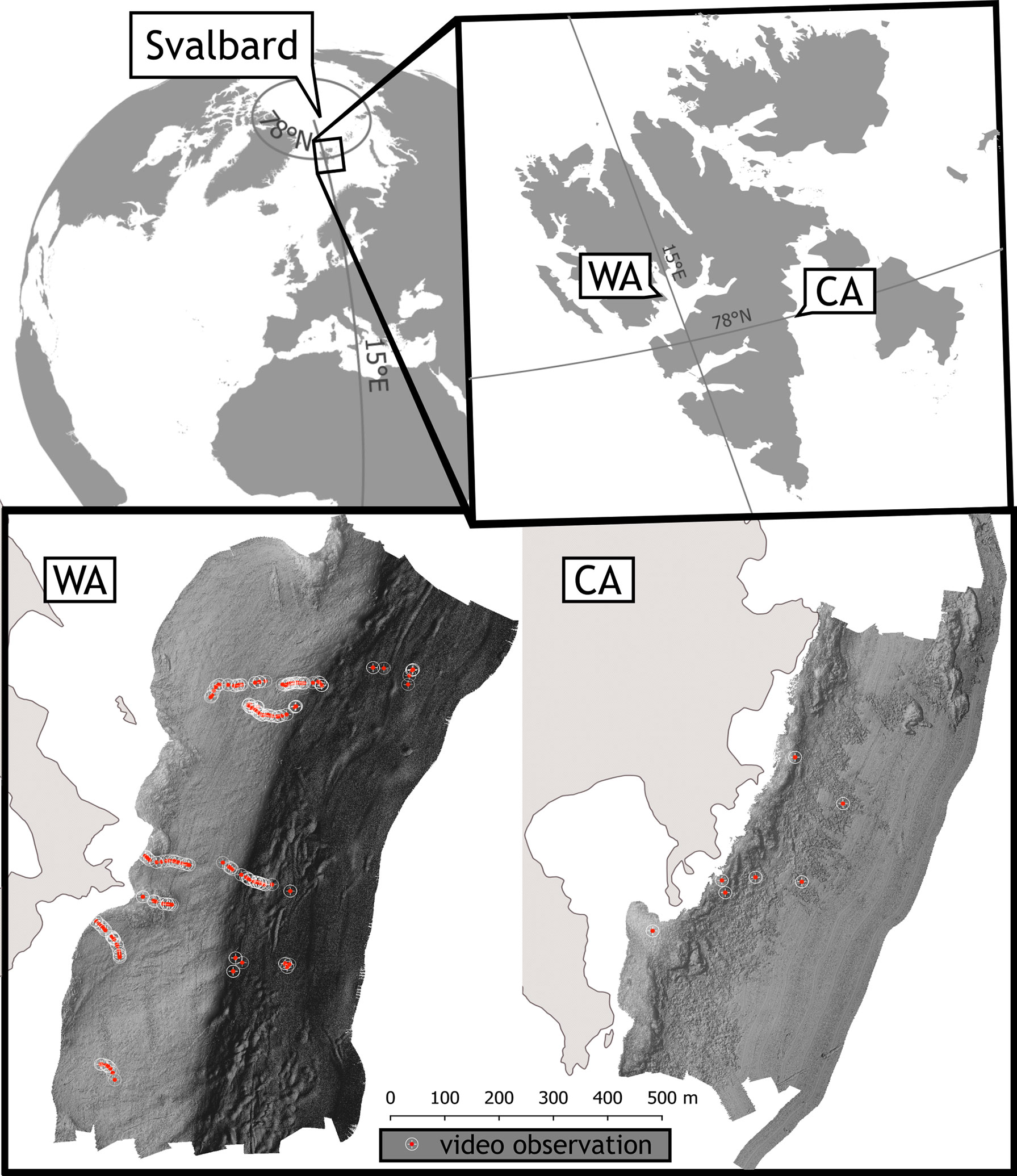
Figure 1 Localization of hydroacoustic study area and ground-truthing data (open circles) over reliefs of surveyed polygons in Isfjorden (Bohemanneset) in West Spitsbergen referred to as Warm Arctic (WA) and in Storfjorden (Agardhbukta) East Spitsbergen referred to as Cold Arctic (CA).

2.2 Data acquisition

2.2.1 Positioning and survey

All acoustic data were collected from small boats with side poles mounting of single beam (SBES) and multibeam (MBES) echosounders on port and starboard side, respectively. There were also two separate positioning systems. A single GNSS antenna was mounted on the top of the SBES pole, while two Trimble antennas were attached along the MBES pole with 2 m separation to secure precise positioning. Due to problems with receiving RTK corrections in remote Arctic areas, we decided to record all navigation and motion data and process them later using Applanix PosPac PP-RTX technology to achieve centimetric horizontal and vertical positioning accuracy. Data were collected from both instruments simultaneously. Survey lines were planned along the shore line starting from the deeper part towards shallower to avoid underwater obstacles such as rocks. Line spacing was adjusted to assure full bottom coverage by the multibeam wide swath system.

2.2.2 Single beam echosounder

Previous theoretical (Carbó and Molero, 1997; Shenderov, 1998) and experimental studies (Sabol et al., 2002; Kruss et al., 2008; Kruss et al., 2017) show that the SBES echo envelopes recorded over rocky, sandy or muddy bottom and seafloor covered by macrophytes are considerably different. Habitats classification based on acoustic mapping from SBES is already a well established technique with efficient and reliable results (Brown et al., 2011).

Acoustic data were recorded at 420kHz frequency by Biosonics DTX split beam echosounder. This echosounder collects data with a swath perpendicular to the bottom with an opening angle of 5.2°. Echoes received come from a round shape area interacting with the incident wave. The deeper it is, the bigger the footprint becomes. This kind of survey gives information from the seabed below the instrument and along the boat track. Data were recorded by Biosonic’s Visual Acquisition software, which stored a full echo signal envelope for each ping as volume backscattering strength values (SV). Based on that, we could analyze bottom reflection and water column reverberations at the same time. Pulse length used was 0.1 ms, giving 2 cm vertical resolution of the data.

Parametrization and classification of seabed substrata was possible due to differences in signal response values and echo shapes originating from different bottom types and habitats (Lurton, 2002; Jackson and Richardson, 2007). Echo signal was corrected for signal losses due to the water, to enable it to estimate the influence of bottom hardness and detect macrophytobenthos growing on it, and to compare the data from different depths.

2.2.3 Multibeam echosounder

We used a high resolution integrated multibeam echosounder Norbit iWBMSh. The instrument was equipped with a motion sensor and set to operate at 360 kHz, with a swath opening of 140° across track, and 1.9° along track. Each swath comprises 512 beams and outputs a point cloud of bottom detections, allowing centimetric resolution of the seabed surface. A range of intensity values were recorded for each beam (snippet) as well, producing a high-resolution backscatter mosaic image (showing how strong the bottom is reflecting acoustic signals). The great advantage of using MBES for habitat mapping is wide coverage while keeping high resolution of the mapped seafloor areas.

Data were collected using QPS QINSy software that records but also visualizes the preliminary results and supports navigation during the survey. Post-processing was made in QIMERA for bathymetry and FMGT for backscatter.

The pre-processed data set gathered by single beam echosounder consists of 69468 observations at the WA and 86126 at the CA. SBES parameters were smoothed with a rolling filter calculating mean, median and extremes of each variable. This dataset was then aggregated into values representing averaged algae and bottom descriptors derived from SBES rasterized into 25 cm x 25 cm ‘pixels’ (0.0625 m²) matching the underlying bathymetric grid (for illustration see Supplementary Figure S1). The value associated with each pixel is determined by calculating statistics for all observations falling within its area. This resulted in 64553 observations at WA (19706 with algae canopy) and 59513 at Cold Site (12062 with algae canopy). Resulting dataset covered area of 3720 m² at CA and 4035 m² at WA.

2.2.4 Video footage

Ground-truthing was accomplished by inspecting video footage recorded by a submersible camera. Two different systems were used. The CA site was inspected by a drop camera unit consisting of two small sport cameras and diving spotlight attached to a self-made rack constructed from PVC pipes equipped with stabilizing fins. In the WA area, pictures were recorded using a towable platform equipped with a camera, LED lights, depth sensor, altimeter and PAR sensor. Due to that, spatial coverage of ground-truthing points in CA is smaller compared to the other site (Figure 2).

FIGURE 2

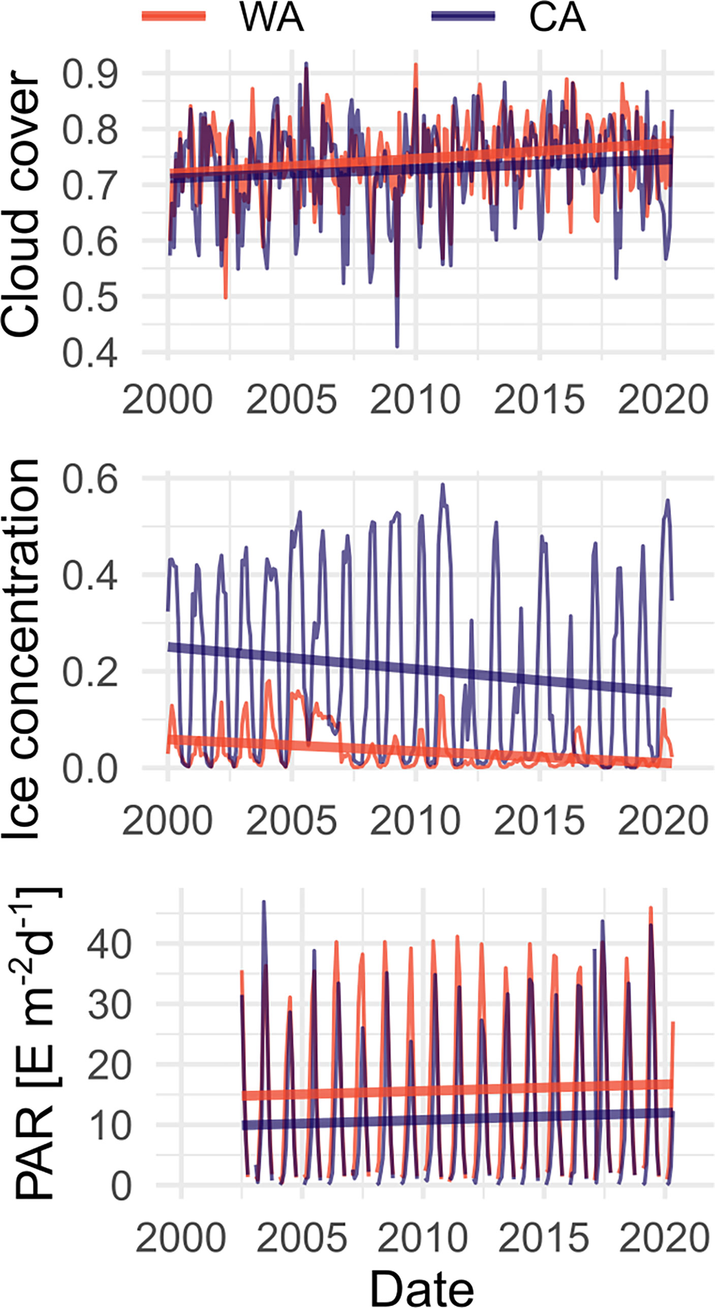
Figure 2 Spatially averaged cloud cover, monthly ice concentration (a fraction of water surface covered by sea ice according to the MERRA-2 model) and Photosynthetically Active Radiation (PAR) in areas surrounding study sites: Warm Arctic (WA) in West Spitsbergen and Cold Arctic (CA) in East Spitsbergen in years 2000-2020 (data used for plotting were obtained using the Giovanni online data system, developed and maintained by the NASA GES DISC). Thick lines show the trend of the value in each place.

In total, 4868 seconds of video footage was recorded for ground-truthing of echograms: 788 s at the CA site and 4080 s at the WA, all along with single beam echosounder (SBES) acquisition which was to improve their positioning and validating classification results.

When the canopy was dense, the bottom type was not visible. In such cases, we assumed it was a hard substrate. When hard substrate was mixed with soft sediments, barren spots could be observed, revealing its nature.

Observations included a coverage, taxonomic composition of visible algae, type of bottom, presence of sea urchins and singular features (like single kelp, rock on a sandy bottom and other objects clearly visible on the echograms; those observations help in future alignment of data acquired by camera with the ones captured with SBES). Spatial information of observations were fitted by aligning them with SBES datasets using reading closest in time to the given observation.

2.2.5 Remote data

Turbidity, diffuse attenuation coefficient for PAR (Kd) and chlorophyll a data presented were based on MODIS-Aqua data provided by NASA OB.DAAC (NASA’s Ocean Biology Distributed Active Archive Center), processed using SeaDAS v2021.1; developed and maintained by NASA Ocean Biology Processing Group (OBPG) (Baith et al., 2001). SeaDAS was modified to use Spectral Shape Parameter (SSP) aerosol correction (Singh et al., 2019). Suspended particulate matter (SPM) were estimated as described in (Nechad et al., 2010) using water-leaving reflectance (ρ_w) at a 667 nm band generated from MODIS-Aqua data using SeaDAS.

Giovanni interface (Beaudoing et al., 2020) was used to acquire data describing environmental conditions in areas around sampling sites (Figure 1). All data used in our research are monthly values, area-averaged in respective areas representing sampling polygon’s surroundings. Cloud cover, expressed as cloud fraction (The fraction of the sky that is covered by clouds) and PAR (4 km resolution) are based on The Level-3 (L3) MODIS Atmosphere Monthly Global Product MYD08_M3 (NASA Goddard Space Flight Center et al., 2018) and ice concentration (sea-ice covered fraction of tile) are based on MERRA-2 product: tavgM_2d_flx_Nx (Global Modeling and Assimilation Office (GMAO), 2015).

2.3 Data processing

2.3.1 SBES data analysis

The database with algae detections from each SBES ping was translated into a spatial database using the raster package (Hijmans and van Etten, 2016) in the R environment. Point data were rasterized using MBES bathymetry as a reference grid with basic resolution of 25 cm (Supplementary Figure S1).

Small boats, like the one used as a platform to collect the presented data, are prone to unpredictable movements due to wave, wind and on-board operations. This influences SBES echoes, as this instrument was not attached to advanced positioning (as it was in a case of MBES using Real Time Kinematic) corrections or motion sensor data. To compensate for the unexpected movement effect, each calculated parameter was smoothed with a median walking window filter (window width = 100 pings).

The echo signal is automatically corrected for transmission loss in the Biosonic’s software, full echograms were output as Matlab (Mathworks) input files for further analysis. Macroalgae detection was performed by procedures developed by Kruss et al. (2017).

Having “roots” (a base of the canopy; depth at which holdfasts are attached to the bottom) and “tops” of macroalgae (the depth of the surface of algal canopy) we could calculate the macroalgae layer thickness expressed in SBES samples, which was subsequently recalculated to be expressed in meters.

Due to a changing velocity of the boat during a data acquisition, the number of pings per output cell varied. To maintain a high quality of the statistical analysis, cells with less than 50 pings were removed. Rasterization processes were performed using a number of aggregating functions: (1) coverage (expressed as number of positive algae detections/all pings within a cell), (2) median canopy thickness, (3) canopy type: 5 categories of canopy described in Table 1.

TABLE 1

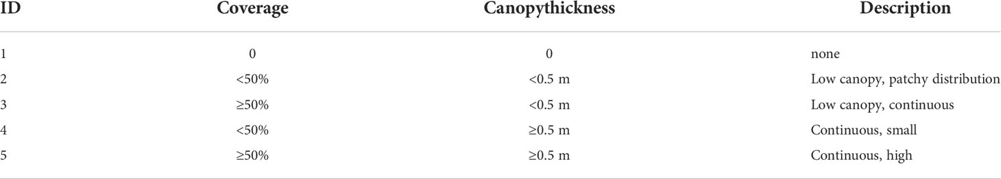
Table 1 Description of canopy categories in the current study.

2.3.2 Bottom type classification

Not every substrate is suitable for algae to grow — it must provide a secure and stable surface to attach to. Herein, we categorized substrates into two categories: hard (including bedrock, boulders and big rocks) and soft (loose sediments like sand and small gravel). In many cases, mixtures of them are observed: e.g. rock on sand etc. Different levels of disturbance would display as different fractions of a potential niche that are actually used by algae (realized niche): the greater the disturbance, the more likely that the canopy would be detached or damaged. In order to compare canopy in two distinct sites, we limit our analysis to hard substrates only.

Seabed classification based on SBES combined with ground truth data is a complex task. We used well established parametric methods based on echo shape descriptions (van Walree et al., 2005; Michaels, 2007; Anderson et al., 2008; Kruss et al., 2017) to estimate bottom hardness and type. These parameters were calculated for each echo envelope (e.g. mean, length, kurtosis, skewness, center of gravity).

We also used a very crude method to discriminate between bottom types. First, mean signal strength of the bottom was calculated for each reading. Those values were then pooled together, and 10000 random values were sampled and fed into a k-means procedure looking for two distinct groups of values (hard and soft bottom). The histogram of SV was clearly bimodal, so doing that would produce results good enough for further analyses (Supplementary Figures S2, S3).

2.3.3 Multibeam data processing and terrain analysis

Norbit multibeam data were treated in QPS QIMERA (multibeam processing software) using processed positioning data with centimetric precision. Together with motion unit data we could compensate for the output bathymetry for all vertical and horizontal artefacts that come from boat movement and refer to this layer to mean water level for the region. Backscatter mosaic was created in QPS FMGT software based on registered snippets. This software automatically corrects transmission losses of the signal and angular dependency of signal reflection, which makes mosaics homogenous and removes artefacts.

Bathymetry was created with 25 cm resolution, keeping sufficient point density per cell. This layer was the basis for further calculation of roughness, slope and aspect as derivatives of bottom morphology.

3 Results

Investigated locations differ by the dose of PAR reaching the bottom. It is a result of the ice cover presence/absence in spring, and the higher concentration of mineral particles associated with the runoff of discharge waters reaching the littoral zone either directly from the glaciers or through the river (Agardhelva), carrying a significant load of suspensions (3.7 mg L^-1 TSS) (van Winden, 2016). Such a load reduces the transparency of the water in CA (in most sites inspected with the camera, visibility was very low). WA, on the other hand, is located far from glaciers, so suspended matter in the water was already significantly diluted by the waters of the open sea penetrating the Isfjorden. At the CA the bottom remains flat below the depth of 20 m what facilitates resuspension of the fine material, what is not a case at the WA where the bottom drops steeply to a depth where the influence of the waves causing the re-suspension of the bottom sediments is negligible.

3.1 Remote sensing of the optical parameters of the water ininvestigated areas

Concentrations of particulate matter were higher at CA for most of the time reaching a value of 20 g m^-2, while in WA this occasionally reached ca. 17 g m^-2, but generally stayed below 8 g m^-2 (Figure 3). Particulate matter was the main driver of overall diffuse attenuation coefficient (K_d) variability, as the chlorophyll a concentrations were similar in both cases. Overall, transparency in both regions was similar (Figure 3).

FIGURE 3

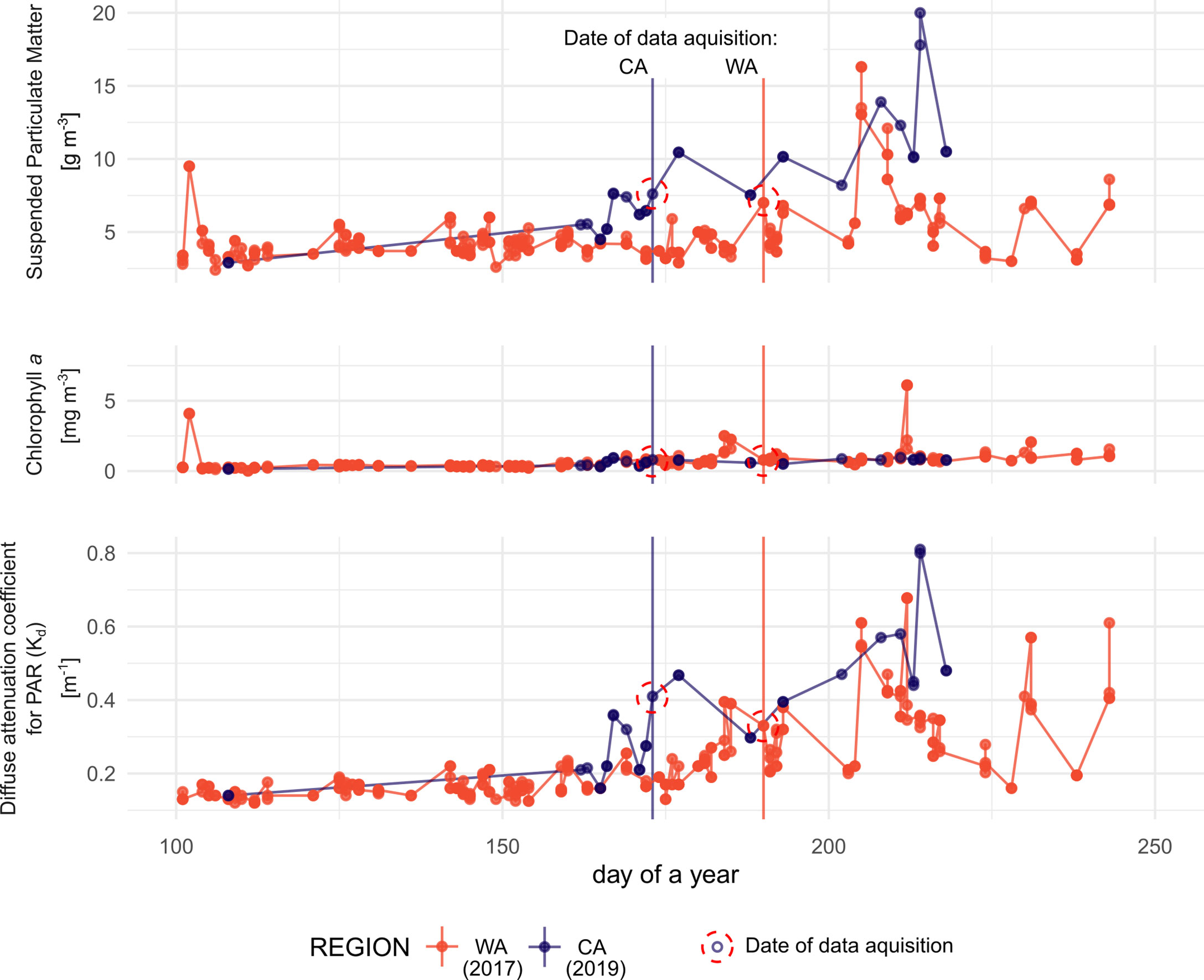
Figure 3 Time series of remotely derived parameters related to water transparency. Each series shows values from the year when the area was surveyed (2017 for WA and 2019 for CA). Day when in situ data were collected are indicated by vertical lines. Lack of data in case of CA in the spring is due to the ice and clouds obstructing the view.

3.2 Background bathymetry

Planimetric areas (measured along sea surface) of 624 327 m² at the WA and 379 000 m² at the CA were surveyed (Table 2). It corresponded with sea floor areas (bottom landscape surface) of 645 950 m² at WA and 396 224 m² at WA.

TABLE 2

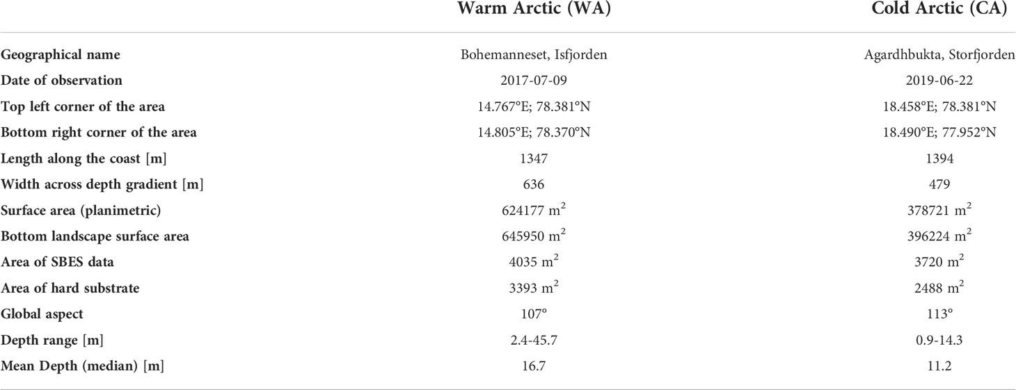
Table 2 Geographical position and physical information of the two study sites Warm Arctic (WA) and Cold Arctic (CA) in respective West and East Spitsbergen.

3.3 Single beam echosounder observations

The best split between hard and soft spatially averaged bottom reflectivity calculated by k-means for two groups performed on the results of rasterization of the local median value of SV was -7.406. Using this criterion most of the hard and soft substrate was correctly classified. Mixed substrates that included soft sediments were also assigned to the soft substrate class using this model (Table 3).

TABLE 3

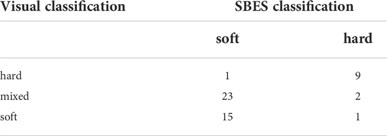
Table 3 Comparison of visual and acoustic classification of bottom.

At the WA 84% of all SBES readings indicated presence of the hard substrate, while in the CA this share was lower — 67%. As data represents averaged values in 25 cm x 25 cm quadrants it corresponded to the areas of 2488 m² in CA (out of total 3720 m²) and 3393 m² in WA (out of total 4035 m²).

More than half of both areas were not inhabited by algae (58% in WA and 59% in CA; Table 4). The most prominent canopy type (continuous and thick) occupied 1[0-9] % of the WA bottom, while it was present only at 2% of a suitable bottom at the CA.

TABLE 4

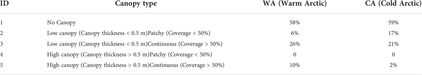
Table 4 Share of different canopy types (according to Table 1) in each studied area.

In both cases, continuous low canopy comprised nearly 25% of the total area of inhabitable bottom (26% vs 21% WA and CA respectively). Patchy low canopy was nearly as common as the continuous one (19%) at CA site, while being limited to 9% at WA.

At the WA site, macroalgal canopies occupied the available bottom to a larger extent compared to CA: at the WA site over 50% of suitable bottom was covered with macrophytes in waters shallower than 6 m, reaching up to 80% at 3 m depth. At CA, it never exceeds 50%, with the peak coverage of 45% at 5 m (Figure 4).

FIGURE 4

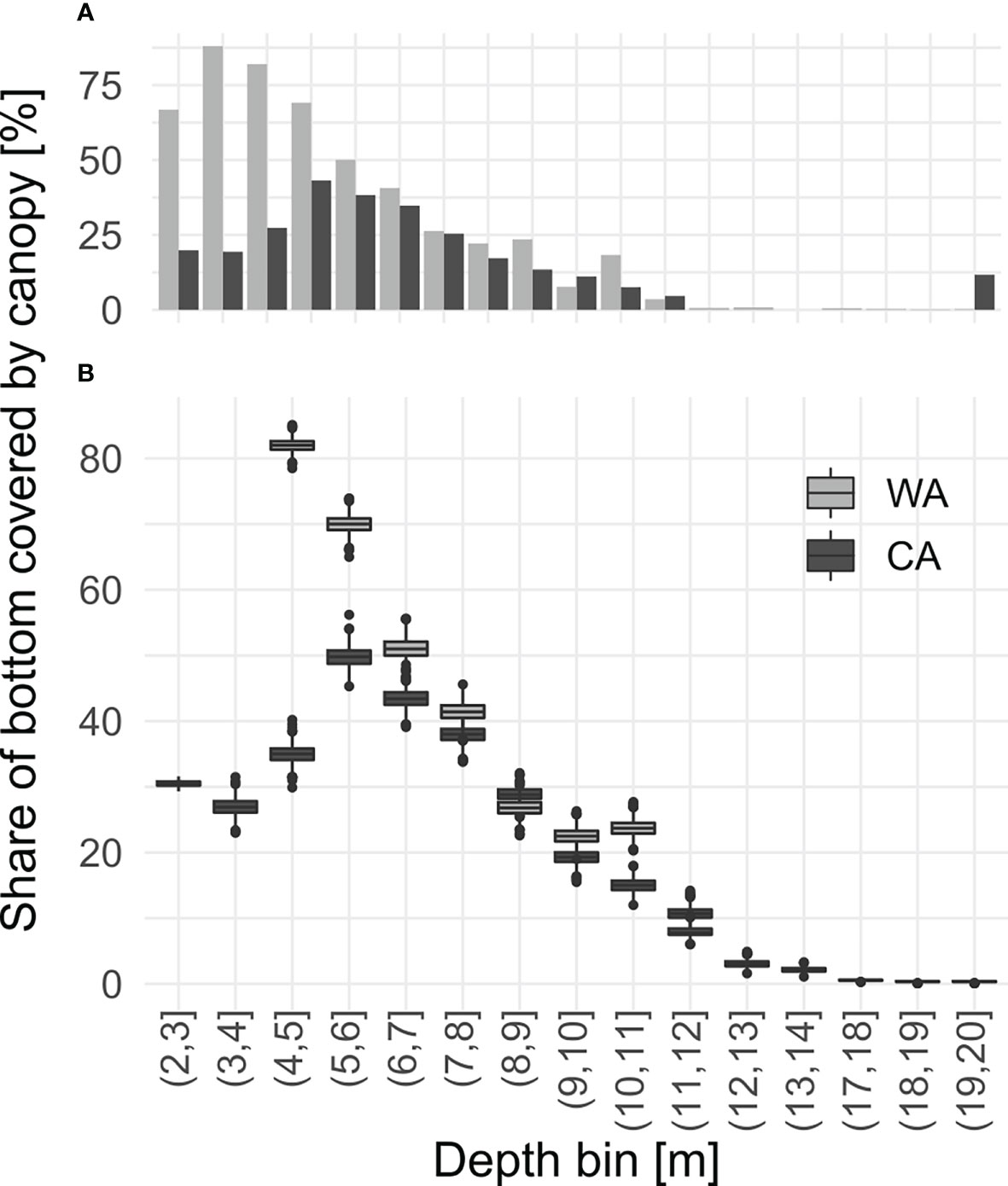
Figure 4 Algal coverages of inhabitable bottom averaged for distinct depth bins in sites Warm Arctic (WA) and Cold Arctic (CA): (A) based on all observations, (B) calculated from 1000 randomly selected samples within the given depth bin permuted 9999 times; boxplots represents distribution of values in all permutations.

Canopies at both sites extended down to 13 m under water surface (coverage >5%). Occasionally some fronds were observed deeper.

Observed canopy thickness ranged between 0.1 m and 1 m (Figure 5). At CA, average canopy thickness was fairly constant throughout the depth range (thickness of 0.25 m - 0.3 m) reaching maximum thickness in the 6 m bin. At WA, peak average canopy thickness was 50 cm reaching maximum thickness in the 4 m depth bin, decreasing to 25-30 cm thickness at 7 m depth. At both study sites the thickest canopy was observed at about 4 m - 5 m depth where values as high as 1 m were recorded (Figure 6).

FIGURE 5

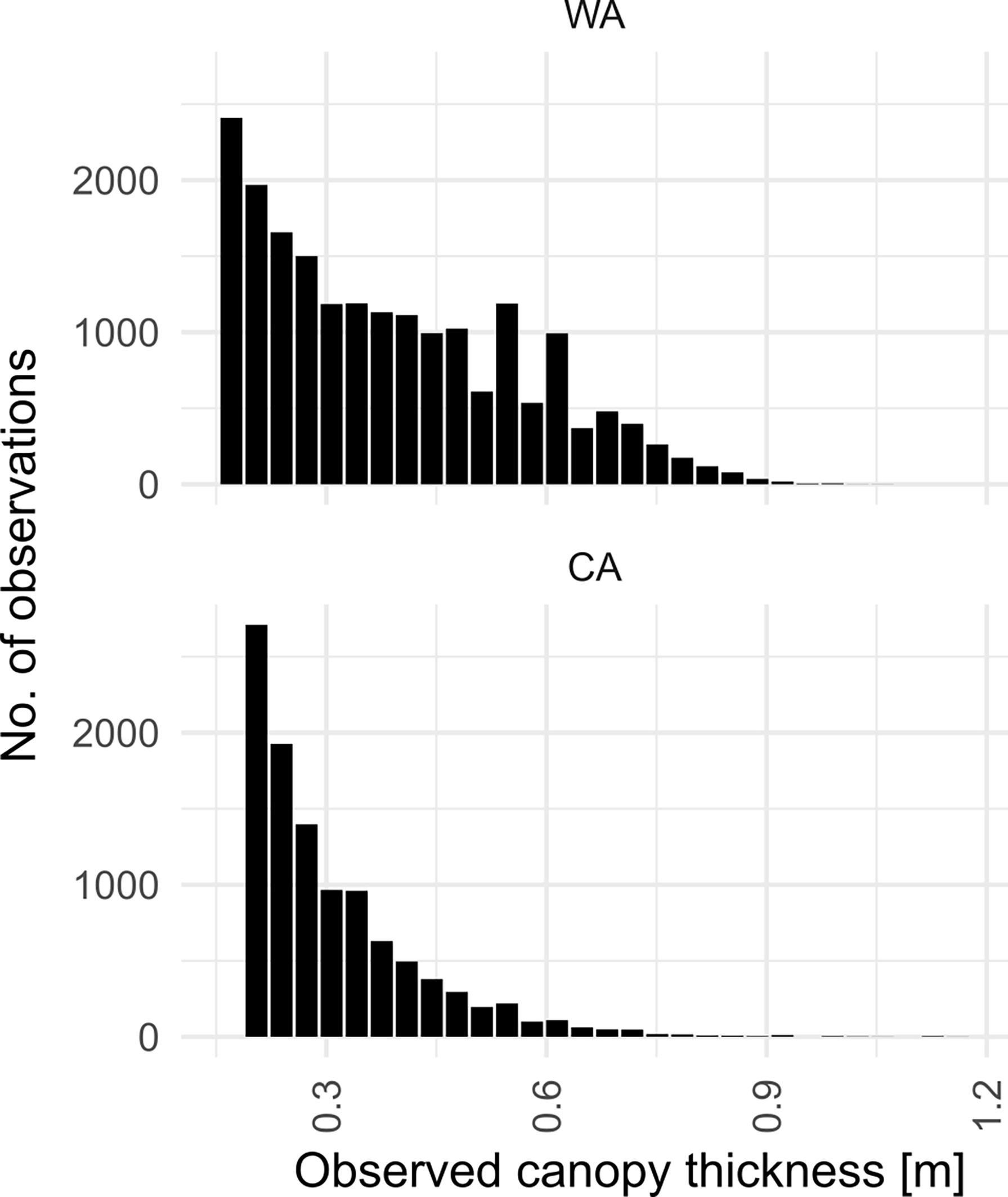
Figure 5 Histograms of canopy thickness observed at studied sites.

FIGURE 6

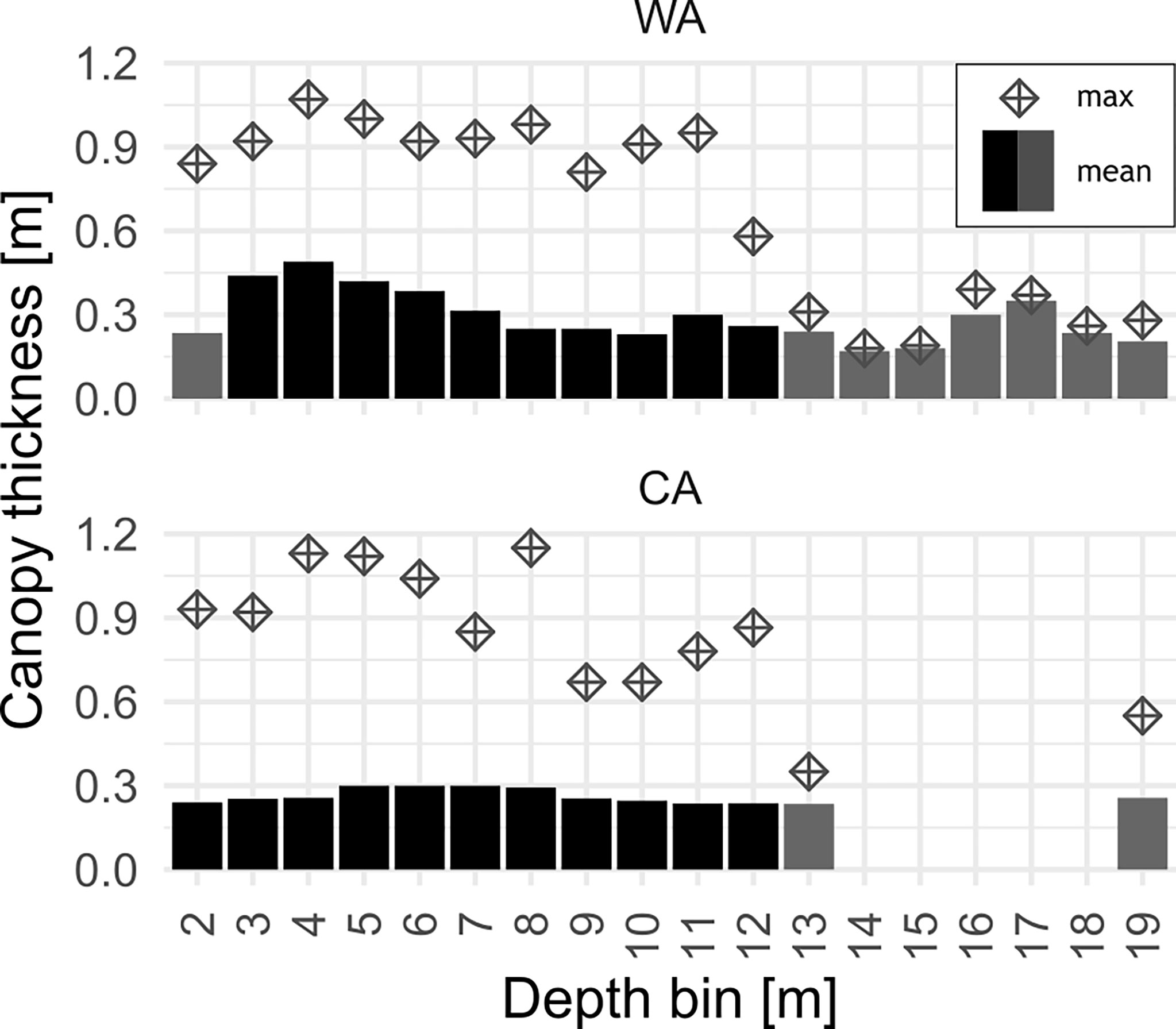
Figure 6 Canopy thickness in depth bins at each station: bars represents mean values, error bar — median canopy thickness and diamond point shows maximal value recorded in each bin. Bins with less than 100 observations were indicated by grey fill.

The canopy was the thickest on average at depth between 3 m – 5 m extending more than 30 cm from the bottom, reaching as much as 50 cm at 4 m (Figure 6). At the CA site, the mean macrophyte canopy layer did not exceed 25 cm at any depth and was constant more or less even down to 7 m.

At WA (Figures 7A–F), continuous high canopy is present whenever there are boulder/rock deposits, while much less frequent on flat areas, which are associated with sedimentary bottom. At CA (Figures 7G–L) high canopy was scarce and scattered with very few localities where it was somehow continuous (present in the number of subsequent pixels). Dark shades of the relief indicated shallow water, getting lighter with increasing depth. In both sets of panels, the coast is located on the top left side of the panel and open water is on the bottom right side. At WA structures extending from the bottom (rock deposits, boulders etc.) are covered with high continuous canopy in most cases (panels a, b, d, f). It is different from the cold scenario (panels g, i, j, k) — high canopy is limited to parts of the structure located deeper. It is clearly seen in k and i panels. Also, at CA high continuous canopy is more likely to be located in between some extending bottom features compared to areas without such protection (panel h).

FIGURE 7

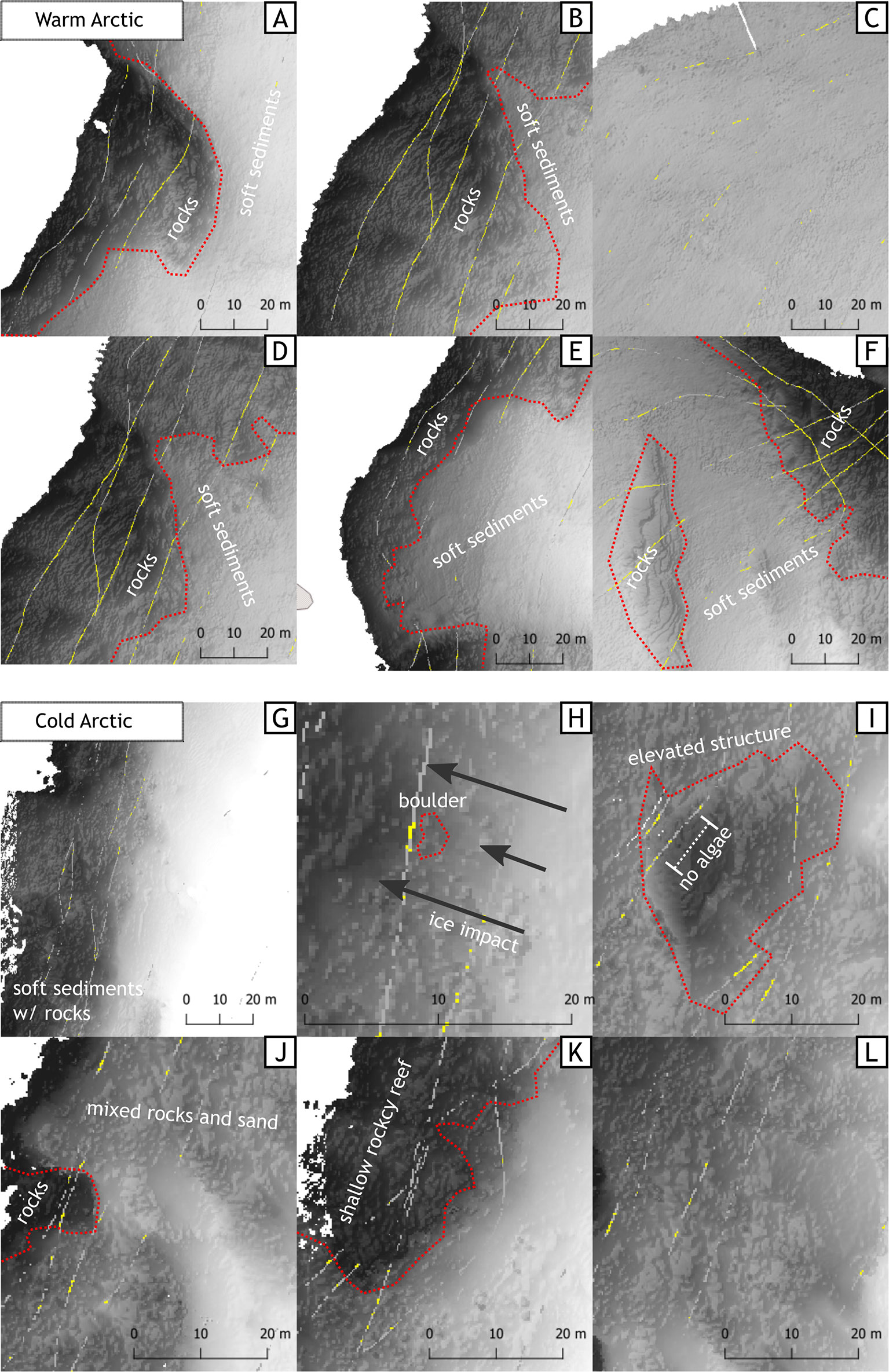
Figure 7 Selected close ups of algae presence along the observation routes indicated by yellow pixels (absence of algae showed in light grey) overlaid on bottom relief. Red lines indicate margins of the bed rock; arrows indicate direction of ice impact (for further explanations see text).

3.4 Video inspection of chosen parts of the investigated areas

All observed individuals were assigned to 18 taxa, 8 of which represented distinct species, 4 represented higher taxonomic affiliation that could not be identified precisely, two included two species that could not be distinguished on visual basis and 4 artificial taxa pooling together species that could only be assigned to higher taxonomic rank than species. The lowest number of species was found at WA with 10 taxa in total, while at CA 15 taxa were observed (Table 4). Altogether, the presence of 13 species of algae were identified on collected video footage. Red algae were represented by 5 and Phaeophyta by 6 taxa (Table 4). Taxa which could not be identified solely on video basis were pooled together into higher taxon.

At the WA site presence of the main kelp grazer — sea urchins — was observed, while no individuals were spotted at the CA site. Sea urchins’ presence was limited to the deeper areas at WA (Table 4).

3.4.1 Species composition

Canopies were dominated by species typical for Arctic and boreal high latitudes of the Atlantic Ocean. The exception was an endemic Arctic species, Laminaria solidungula, which was observed at both sites. The most frequently observed species of macroalgae were kelps: Alaria esculenta, Laminaria digitata/hyperborea and Desmarestia aculeata. Distinction between L. digitata and L. hyperborea solely on visual inspection of recorded material was not possible. For that reason we pooled those taxa into one entity.

At WA 8 brown algae and one red algae (Lithothamnion sp.) were identified, while at CA 7 taxa of brown algae and 5 of red algae were observed (Table 5).

TABLE 5

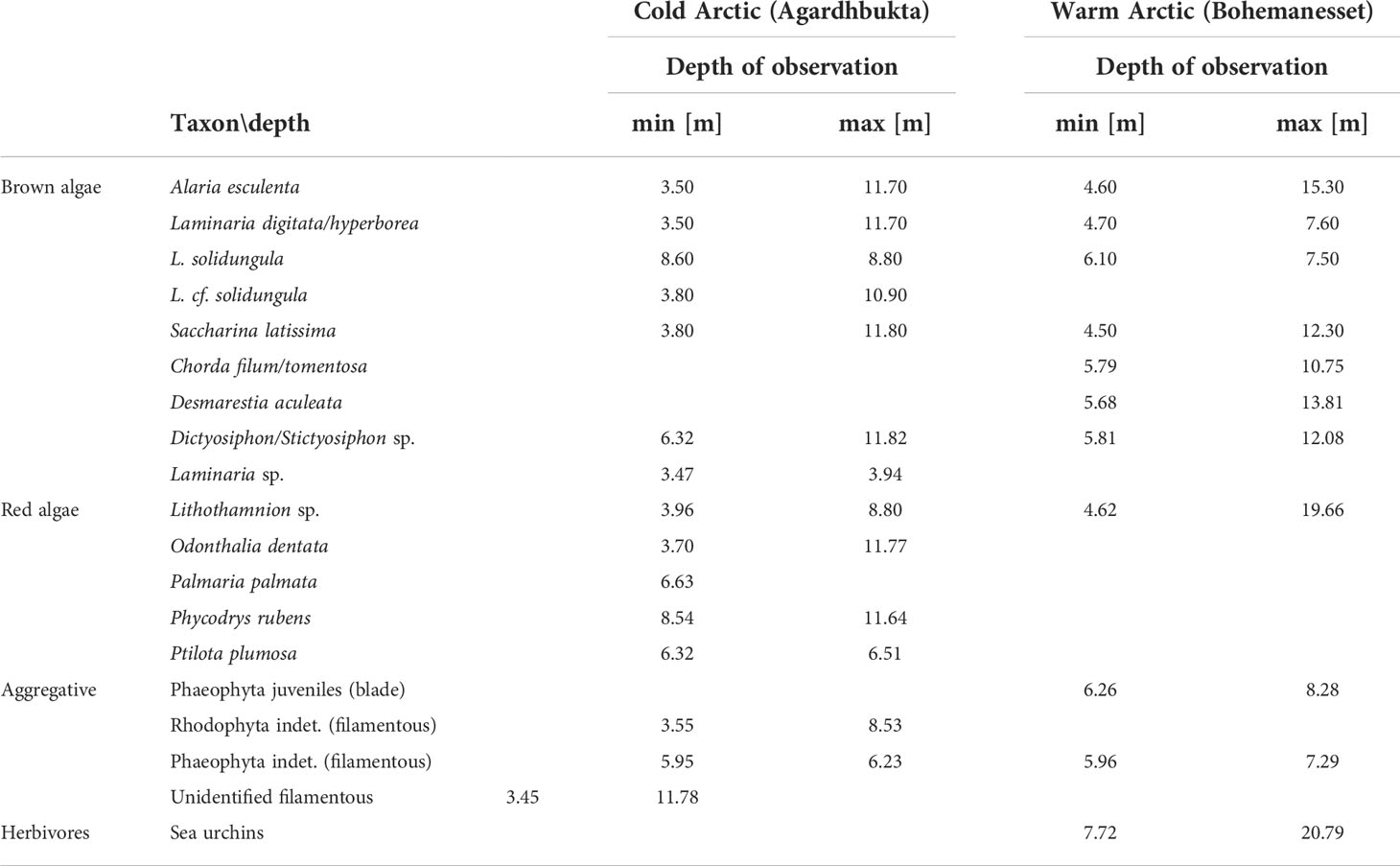
Table 5 List of taxa observed on video records.

4 Discussion

Species composition list recorded in this study is much shorter than the checklist reported by comprehensive floristic studies in the area. Here, we identified 18 out of 83 species found previously (Fredriksen and Kile, 2012) in waters of the west Spitsbergen in the supralitoral, eulittoral (intertidal) and subtidal zones combined. The lower number of species identified here was due to the different methods we used. We identified the species based on visual inspection of the underwater footage, thus, only abundant species larger than 10 cm in size could be accurately identified. Our conclusions are derived specifically from the patterns of algae distribution, not from their species richness. Therefore, our method allowed us to collect relevant data quicker and over a much larger area than traditional methods, such as bottom dredging and scuba diving.

The macroalgal community in the surveyed places consisted of the same dominant kelp species as ones observed in adjacent areas: in Hornsund located south of WA (where combined biomass of Laminaria digitata, Saccharina latissima and Alaria esculenta accounts for over 70% of the total macroalgal biomass) (Tatarek et al., 2012) and in Kongsfjorden (Bartsch et al., 2016; Kruss et al., 2017).

At WA kelp grazers were observed. In deep water areas many individuals of sea urchins were found, whose presence shaped the lower depth limit of the kelp forest. Sea urchins are known to be the only herbivores able to graze on kelps to the point that they control its distribution. In extreme cases, when the population of sea urchins exceeds a certain threshold (>500 ind. m^2), the grazing exceeds kelps’ ability to recover and their population collapses leaving barren zones (Scheibling et al., 1999; Gagnon et al., 2004). The water dynamics and presence of predation excludes sea urchins from shallow waters, therefore, the effect of sea urchins on kelps is only present starting from a certain depth. Since differences between canopies in deeper areas were not very pronounced (especially when it comes to space utilization) we conclude that sea urchins have no significant top down control in considered areas.

Sea bottom is similar at both study sites. In shallow water areas (< 5 m) it is mostly hard with exposed bedrock and deposits of boulders and large stones, while deeper regions (>5 m) are covered with finer sediments like sand and mud. Bottom at WA is steeper compared to CA, which is generally very flat: average slope at WA is 2.06° (SD = 0.8), while at CA it is 0.05° (SD = 0.07). At greater slopes sediments are more likely to be transported into deeper water, which makes macroalgae less likely to be buried underneath (Duarte, 1996; Krause-Jensen and Duarte, 2016)

In both areas, less than a half of the surface identified as suitable for macroalgal canopy development was inhabited by algae and was nearly identical between two sites — 42% at WA and 41% at CA. Similar values were reported for nearby locations: 41% in Kongsfjorden (Tatarek et al., 2012; Kruss et al., 2017), 29% in Hornsund (Kruss, 2010).

We simplified the classification method compared with other studies that were specifically aimed to precisely describe bottom hardness and sediment types (LeBlanc et al., 1992; Kostylev et al., 2001; Kenny et al., 2003; Passlow et al., 2006; Longdill et al., 2007; Bartholomä et al., 2011; Haris et al., 2012; Diesing et al., 2014). Bottom hardness is the main factor influencing its ability to reflect acoustic waves, however this property is modified by a number of factors such as: layer of fine sediments covering hard bottom, stones covering fine substrate, vegetation, or orientation of the bottom surface. To decrease the effect of those modifiers, SBES readings were spatially aggregated. In our case, the distribution of aggregated reverberated signal strength was clearly bimodal, which corresponded to two bottom types present within studied areas: hard rocky bottom and soft sedimentary bottom. Indeed, by fitting the data with different runs of k-means, we achieved the best fit with the model with two classes (chosen by the mean silhouette width criterion). It resulted in a conservative split where only bedrock, boulders and dense stone beds were recognized as hard substrate, while mixed types like stones on sand and fine gravels were classified as soft substrate. While some algae were observed on bottom of mixed type, they did not form dense canopies. Therefore, we concluded that excluding those places from the analysis did not change the overall conclusions.

Continuous and high macrophyte canopy was more frequent at WA with 10% coverage of habitable surface, compared to only 2% coverage of suitable substrate at CA. Thicker (>0.5 m) canopies were only observed in areas where coverage reached more than 5% of suitable habitat. Such high meadows can only be formed at undisturbed bottom (no scouring) by fully developed kelps growing close to each other. Solitary kelps lay flat on the bottom, rather than extend upright toward the surface (species that in the study area lack features facilitating buoyancy), thus its apparent height (measured with SBES as canopy thickness) would not be much more than the height of its strip. Individuals growing in dense canopy, in turn, support each other and thus form a thicker canopy.

Canopy at WA was better developed than the one observed at CA. Fronds at WA were big, regularly shaped, without any apparent damage (Supplementary Figure S4). Kelps covered most of the bottom where the substrate was made of bedrock or large boulders. Often, numerous blades were extending from rhizoids clustered together. On very few occasions we observed species of different kelps present in the same place – individuals of given species were grouped with each other, but such patches did not display any kind of zonation. Hardly ever Desmarestia aculeata occurred when kelps were present, while this species was very common there substrate contained stones and/or gravel too small to support kelps to keep their fronds in place.

The canopy thickness reached maximum value at depths between 3 m and 5 m. In the case of WA it is possible that more data from shallow water could potentially shift the distribution towards shallow water making the discrepancy between study sites more apparent. At WA shallow bottom is utilized to much higher degree than at CA which is most probably caused by the ice-scouring damaging older fronds. Below 6 m depth there is no difference in share of occupied space in both places, which suggests that this was the maximum depth of ice disturbance. A fully developed seaweed forest was observed at WA mainly in shallow water (less than 6 m), thus in the range of the observed depth of interaction with the ice at CA. This may explain the fact that there are few areas where a dense seaweed forest has been observed.

Interestingly, a similar pattern of the kelp distribution shifting towards shallower waters was observed in Kongsfjorden (Svalbard) where the biomass of kelp peaked around 5 m in 1988 and shifted to 2.5 m recently as a result of warming of the environment, namely: decreased ice-scouring and longer photic season allowing algae to occupy shallower areas, and increased turbidity limiting the amount of radiation available in deeper areas (Bartsch et al., 2016; Bischof et al., 2019b).

In heavy ice-scoured areas of the Canadian Arctic (Heine, 1989), where ice impact was observed down to 12 m, perennial algae presence was limited to crevasses and sloping bottoms, while macrophytes were nearly completely removed from exposed surfaces shallower than that. Algal community present there was different to one observed in this study, but it also consisted of Laminaria and Alaria species of similar body type, so they are expected to respond in the same way to the similar environmental pressures.

Destructive events in exposed areas of the sea bottom limit biomass of kelp species, which in turn limits new production in such areas (Filbee-Dexter et al., 2021). Those empty spaces can be utilized by ephemeral algae that are normally outcompeted by perennial species which results in higher species diversity of such a disturbed area (Dial and Roughgarden, 1998). We believe that the high number of observed species at CA can be explained by environmental restrictions on perennial species due to sea ice scouring

Along with the ongoing changes in the climatic system more Arctic coasts will experience sea ice loss. It will result in an increase of areas covered with continuous macroalgal canopy. As disturbance events (ice-scouring in this case) become less frequent, the ephemeral algae will have fewer opportunities to find suitable space, therefore their abundances will most likely decrease and overall we expect a lower macroalgae richness as a consequence of climate warming. Without ice-scouring, algae form much denser meadows — multilayered structures of many individuals intermixed with each other creating safe spaces for associated fauna to live in, protected from water dynamics and predators. By growing in close proximity, kelps give each other support dissipating environmental stresses among many individuals.

Obtained results are preliminary – we have studied one site in each region. We have made an effort to select the most representative sites, however living organisms experience conditions that are the result of complex interplay of many factors, some of which are hard to predict, and to control. It is possible that, despite expectations, areas we have selected to investigate were under conditions that deviate from typical.

The biggest change is expected to occur in shallow waters. Ice-scoured areas shallower than 5 m are strongly underutilized, so macrophytes released from ice pressure will increase their standing stocks to a greater extent. The sea bottom at low depth is affected by waves much stronger than bottom at greater depth. Waves rubbing macrophytes’ thalli against the bottom causes fronds fragmentation which is released to the water column allowing for transfer of organic carbon produced by macroalgae into the pelagic system. This might lead to increased primary production of kelp forests, as declining ice would allow them to use previously underutilized space where a higher amount of energy is available. Interaction with water dynamics would release a lot of this new production into adjacent systems. On the other hand, kelps compete for nutrients with planktonic primary producers and, living at the bottom, where the resuspension occurs, do it in a very efficient way (Jiang et al., 2020). Inhabiting shallower water would make them more exposed to extreme events that would facilitate the process of their export into the deep water areas, where they are deposited as blue carbon, acting as a carbon pump, or onto the land, where they are built into terrestrial food chains.

5 Conclusions

1. There is a difference between macroalgal canopies present in the warm and cold study sites both in qualitative and quantitative terms.

2. In warm scenarios, exposed areas are more likely to be covered by a high, continuous vegetation than in cold areas.

3. Ice-scouring is a prominent source of damage to the frond, manifested in the cold areas.

4. Higher environmental pressure at the CA site leads to higher species diversity with turf algae utilizing barren spaces in between kelps fronds. Stable conditions at the WA site lead to more uniform kelp coverage and to segregation between dominant species.

5. As there is less ice cover in the cold regions of Svalbard kelp forests most probably will broaden its extent towards shallower waters and utilize more available surface increasing overall density of kelp forest.

Data availability statement

The raw data supporting the conclusions of this article will be made available by the authors, without undue reservation.

Author contributions

JMWjr. was responsible for method design, data collection, data analysis, and writing a manuscript. JMW and JS applied for money, organized an expedition, collected data and supervised works on manuscript. AT collected data and analyzed video footage. AK was responsible for all hydroacoustics data and RS analyzed MODIS data. All authors contributed to the article and approved the submitted version.

Funding

This research was funded through the 2017-2018 Belmont Forum and BiodivERsA joint call for research proposals, under the BiodivScen ERA-Net COFUND programme, and with the funding organisations Research Council of Norway (project nr. 296836 and National Science Centre Poland (project nr. UMO-2015/17/B/NZ8/02473).

Acknowledgement

We would like to thank Jakub Wiktor, Michał Strach and Bożena Skrzydlińska for reading and commenting on the manuscript. We would like to thank reviewers for taking the time and effort necessary to review the manuscript. We sincerely appreciate all valuable comments and suggestions, which helped us to improve the quality of the manuscript. We would like to acknowledge NASA OB.DAAC for providing satellite (MODIS-Aqua) data and NASA OBPG for developing and maintaining SeaDAS. PAR, cloud cover and ice concentrations were obtained and aggregated with the Giovanni online data system, developed and maintained by the NASA GES DISC. We also acknowledge the MODIS mission scientists and associated NASA personnel for the production of the data used in this research effort. Norbit Subsea and QPS made this study possible by sharing multibeam equipment and processing software.

Conflict of interest

Author AK is employed by NORBIT.

The remaining authors declare that the research was conducted in the absence of any commercial or financial relationships that could be construed as a potential conflict of interest.

Publisher’s note

All claims expressed in this article are solely those of the authors and do not necessarily represent those of their affiliated organizations, or those of the publisher, the editors and the reviewers. Any product that may be evaluated in this article, or claim that may be made by its manufacturer, is not guaranteed or endorsed by the publisher.

Supplementary material

The Supplementary Material for this article can be found online at: https://www.frontiersin.org/articles/10.3389/fmars.2022.1021675/full#supplementary-material

Supplementary Figure 1 | Example of rasterization results. Square mesh is 25 cm x 25 cm aligned with a bathymetry grid (here visualised with hillshade procedure to highlight bottom features) on different scales. Each pixel has a value when there is at least one SBES ping (red dots on panel c) within its limits. In this example, the canopy type category is presented. (A) aggregation results on a scale of study area (here: part of WA site), (B) conceptual diagram of procedure and (C) the real-life analogous case.

Supplementary Figure 2 | Histogram of bottom mSv values at both areas. Readings are split into ones without canopy and ones with one. Over-representation of values close to zero (hence with higher ability to reflect acoustic waves) is due to our focus on canopy, which is linked to hard substrate.

Supplementary Figure 3 | Optimal number of clusters for k-means procedure on rolling median averaged mean signal level reflected on sediments.

Supplementary Figure 4 | Example snapshots (for more information see text).

References

Andersen G. S., Pedersen M. F., Nielsen S. L. (2013). Temperature acclimation and heat tolerance of photosynthesis in Norwegian saccharina latissima (Laminariales, phaeophyceae). J. Phycol. 49, 689–700. doi: 10.1111/jpy.12077

PubMed Abstract | CrossRef Full Text | Google Scholar

Anderson J. T., Van Holliday D., Kloser R., Reid D. G., Simard Y. (2008). Acoustic seabed classification: current practice and future directions. ICES J. Mar. Sci. 65, 1004–1011. doi: 10.1093/icesjms/fsn061

CrossRef Full Text | Google Scholar

Baith K., Lindsay R., Fu G., McClain C. R. (2001). Data analysis system developed for ocean color satellite sensors. Eos 82, 202–202. doi: 10.1029/01eo00109

CrossRef Full Text | Google Scholar

Bartholomä A., Holler P., Schrottke K., Kubicki A. (2011). Acoustic habitat mapping in the German wadden Sea–comparison of hydro-acoustic devices. J. Coast. Res 1–5. https://www.jstor.org/stable/26482121

Google Scholar

Bartsch I., Paar M., Fredriksen S., Schwanitz M., Daniel C., Hop H., et al. (2016). Changes in kelp forest biomass and depth distribution in kongsfjorden, Svalbard, between 1996–1998 and 2012–2014 reflect Arctic warming. Polar Biol. 39, 2021–2036. doi: 10.1007/s00300-015-1870-1

CrossRef Full Text | Google Scholar

Beaudoing H., Rodell M., NASA/GSFC/HSL (2020) GLDAS Noah land surface model L4 monthly 0.25 x 0.25 degree V2.1 (Greenbelt, Maryland, USA: Goddard Earth Sciences Data and Information Services Center (GES DISC) (Accessed 06-07-2022).

Google Scholar

Bekkby T., Rinde E., Gundersen H., Norderhaug K. M., Christie H. (2014). Length, strength and water flow: Relative importance of wave and current exposure on morphology in kelp laminaria hyperborea. Mar. Ecol. Prog. Ser. 506, 61–70. doi: 10.3354/meps10778

CrossRef Full Text | Google Scholar

Bischof K., Buschbaum C., Fredriksen S., Gordillo F. J. L., Heinrich S., Jiménez C., et al. (2019a). “Kelps and environmental changes in kongsfjorden: Stress perception and responses,” in The ecosystem of kongsfjorden, Svalbard. Eds. Hop H., Wiencke C. (Cham: Advances in Polar Ecology Springer), 373–422. doi: 10.1007/978-3-319-46425-1_10

CrossRef Full Text | Google Scholar

Bischof K., Convey P., Duarte P., Gattuso J. P. (2019b). “Kongsfjorden as harbinger of the future Arctic: Knowns, unknowns and research priorities,” in The ecosystem of kongsfjorden, Svalbard. (Cham: Advances in Polar Ecology Springer) doi: 10.1007/978-3-319-46425-1_14

CrossRef Full Text | Google Scholar

Blondel P., Murton B. (1997) Handbook of seafloor sonar imagery. Available at: https://www.semanticscholar.org/paper/e91bafb2dc2cf694fa542b8659ac9d0becb9d7cb (Accessed December 1, 2021).

Google Scholar

Boertmann D., Mosbech A., Schiedek D., Dünweber M. (2013) Disko west. a strategic environmental impact assessment of hydrocarbon activities. Available at: https://www.forskningsdatabasen.dk/en/catalog/2389318069.

Google Scholar

Bonsell C., Dunton K. H. (2018). Long-term patterns of benthic irradiance and kelp production in the central Beaufort sea reveal implications of warming for Arctic inner shelves. Prog. Oceanography 162, 160–170. doi: 10.1016/j.pocean.2018.02.016

CrossRef Full Text | Google Scholar

Brown C. J., Smith S. J., Lawton P., Anderson J. T. (2011). Benthic habitat mapping: A review of progress towards improved understanding of the spatial ecology of the seafloor using acoustic techniques. Estuar. Coast. Shelf Sci. 92, 502–520. doi: 10.1016/j.ecss.2011.02.007

CrossRef Full Text | Google Scholar

Buchholz C. M., Wiencke C. (2016). Working on a baseline for the kongsfjorden food web: production and properties of macroalgal particulate organic matter (POM). Polar Biol. 39, 2053–2064. doi: 10.1007/s00300-015-1828-3

CrossRef Full Text | Google Scholar

Byrnes J. E., Reed D. C., Cardinale B. J., Cavanaugh K. C., Holbrook S. J., Schmitt R. J. (2011). Climate-driven increases in storm frequency simplify kelp forest food webs. Glob. Change Biol. 17, 2513–2524. doi: 10.1111/j.1365-2486.2011.02409.x

CrossRef Full Text | Google Scholar

Carbó R., Molero A. C. (1997). Scattering strength of a gelidium biomass bottom. Appl. Acoust. 51, 343–351. doi: 10.1016/S0003-682X(97)00012-1

CrossRef Full Text | Google Scholar

Castellani G., Veyssière G., Karcher M., Stroeve J., Banas S. N., Bouman A. H., et al. (2022). Shine a light: Under-ice light and its ecological implications in a changing Arctic ocean. Ambio 51, 307–317. doi: 10.1007/s13280-021-01662-3

PubMed Abstract | CrossRef Full Text | Google Scholar

Dial R., Roughgarden J. (1998). Theory of marine communities: The intermediate disturbance hypothesis. Ecology 79, 1412–1424. doi: 10.1890/0012-9658(1998)079[1412:tomcti]2.0.co;2

CrossRef Full Text | Google Scholar

Diesing M., Green S. L., Stephens D., Lark R. M., Stewart H. A., Dove D. (2014). Mapping seabed sediments: Comparison of manual, geostatistical, object-based image analysis and machine learning approaches. Cont. Shelf Res. 84, 107–119. doi: 10.1016/j.csr.2014.05.004

CrossRef Full Text | Google Scholar

Duarte C. M. (1996) The fate of marine autotrophic production. Available at: https://play.google.com/store/books/details?id=y1RkuAAACAAJ.

Google Scholar

Filbee-Dexter K., MacGregor K. A., Lavoie C., Garrido I., Goldsmit J., de la Guardia L. C., et al. (2021) Sea Ice and substratum shape extensive kelp forests in the Canadian Arctic. Available at: https://ecoevorxiv.org/t82cf/.

Google Scholar

Filbee-Dexter K., Wernberg T., Norderhaug K. M., Ramirez-Llodra E., Pedersen M. F. (2018). Movement of pulsed resource subsidies from kelp forests to deep fjords. Oecologia 187, 291–304. doi: 10.1007/s00442-018-4121-7

PubMed Abstract | CrossRef Full Text | Google Scholar

Fortes M. D., Lüning K. (1980). Growth rates of north Sea macroalgae in relation to temperature, irradiance and photoperiod. Helgoländer Meeresuntersuchungen 34, 15–29. doi: 10.1007/BF01983538

CrossRef Full Text | Google Scholar

Fredriksen S., Kile M. R. (2012). The algal vegetation in the outer part of isfjorden, spitsbergen: revisiting per svendsen’s sites 50 years later. Polar Res. 31, 17538. doi: 10.3402/polar.v31i0.17538

CrossRef Full Text | Google Scholar

Gagnon P., Himmelman J. H., Johnson L. E. (2004). Temporal variation in community interfaces: kelp-bed boundary dynamics adjacent to persistent urchin barrens. Mar. Biol. 144, 1191–1203. doi: 10.1007/s00227-003-1270-x

CrossRef Full Text | Google Scholar

Global Modeling and Assimilation Office (GMAO) (2015) MERRA-2 tavgM_2d_flx_Nx: 2d,Monthly mean,Time-Averaged,Single-Level,Assimilation,Surface flux diagnostics V5.12.4 (Greenbelt, MD, USA: Goddard Earth Sciences Data and Information Services Center (GES DISC) (Accessed 06-07-2022).

Google Scholar

Haris K., Chakraborty B., Ingole B., Menezes A., Srivastava R. (2012). Seabed habitat mapping employing single and multi-beam backscatter data: A case study from the western continental shelf of India. Cont. Shelf Res. 48, 40–49. doi: 10.1016/j.csr.2012.08.010

CrossRef Full Text | Google Scholar

Heine J. N. (1989). Effects of ice scour on the structure of sublittoral marine algal assemblages of st. Lawrence and st. Matthew islands, Alaska. Mar. Ecol. Prog. series. 52, 253–260. Oldendorf. doi: 10.3354/meps052253

CrossRef Full Text | Google Scholar

Hijmans R. J., van Etten J. (2016). Raster: Geographic data analysis and modeling to pakiet R. Package version 2. Available at: https://cran.r-project.org/web/packages/raster/raster.pdf

Google Scholar

Jackson D. R., Richardson M. D. (2007). High-frequency seafloor acoustics (New York: Springer). doi: 10.1007/978-0-387-36945-7

CrossRef Full Text | Google Scholar

Jiang Z., Liu J., Li S., Chen Y., Du P., Zhu Y., et al. (2020). Kelp cultivation effectively improves water quality and regulates phytoplankton community in a turbid, highly eutrophic bay. Sci. Total Environ. 707, 135561. doi: 10.1016/j.scitotenv.2019.135561

PubMed Abstract | CrossRef Full Text | Google Scholar

Kenny A. J., Cato I., Desprez M., Fader G., Schüttenhelm R. T. E., Side J. (2003). An overview of seabed-mapping technologies in the context of marine habitat classification☆. ICES J. Mar. Sci. 60, 411–418. doi: 10.1016/s1054-3139(03)00006-7

CrossRef Full Text | Google Scholar

Kostylev V. E., Todd B. J., Fader G. B. J., Courtney R. C., Cameron G. D. M., Pickrill R. A. (2001). Benthic habitat mapping on the scotian shelf based on multibeam bathymetry, surficial geology and sea floor photographs. Mar. Ecol. Prog. Ser. 219, 121–137. doi: 10.3354/meps219121

CrossRef Full Text | Google Scholar

Krause-Jensen D., Duarte C. M. (2016). Substantial role of macroalgae in marine carbon sequestration. Nat. Geosci. 9, 737–742. doi: 10.1038/ngeo2790

CrossRef Full Text | Google Scholar

Krause-Jensen D., Marbà N., Olesen B., Sejr M. K., Christensen P. B., Rodrigues J., et al. (2012). Seasonal sea ice cover as principal driver of spatial and temporal variation in depth extension and annual production of kelp in Greenland. Glob. Change Biol. 18, 2981–2994. doi: 10.1111/j.1365-2486.2012.02765.x

CrossRef Full Text | Google Scholar

Krumhansl K. A., Okamoto D. K., Rassweiler A., Novak M., Bolton J. J., Cavanaugh K. C., et al. (2016). Global patterns of kelp forest change over the past half-century. Proc. Natl. Acad. Sci. U. S. A. 113, 13785–13790. doi: 10.1073/pnas.1606102113

PubMed Abstract | CrossRef Full Text | Google Scholar

Kruss A. (2010). Akustyczna identyfikacja habitatów bentosowych Arktyki. 38(2):205–229

Google Scholar

Kruss A., Blondel P., Tegowski J., Wiktor J., Tatarek A. (2008). Estimation of macrophytes using single-beam and multibeam echosounding for environmental monitoring of Arctic fjords (Kongsfjord, West Svalbard island). J. Acoust. Soc Am. 123, 3213–3213. doi: 10.1121/1.2933397

CrossRef Full Text | Google Scholar

Kruss A., Tęgowski J., Tatarek A., Wiktor J., Blondel P. (2017). Spatial distribution of macroalgae along the shores of kongsfjorden (West spitsbergen) using acoustic imaging. Pol. Polar Res 38, 205–229. doi: 10.1515/popore-2017-0009

CrossRef Full Text | Google Scholar

Kruss A., Wiktor J. Jr, Wiktor J., Tatarek A. (2019). “Acoustic detection of macroalgae in a dynamic Arctic environment (Isfjorden, West spitsbergen) using multibeam echosounder,” in 2019 IEEE Underwater Technology (UT). (New York: IEEE), 1–7. doi: 10.1109/UT.2019.8734323

CrossRef Full Text | Google Scholar

LeBlanc L. R., Mayer L., Rufino M., Schock S. G., King J. (1992). Marine sediment classification using the chirp sonar. J. Acoust. Soc Am. 91, 107–115. doi: 10.1121/1.402758

CrossRef Full Text | Google Scholar

Longdill P. C., Healy T. R., Black K. P., Mead S. T. (2007). Integrated sediment habitat mapping for aquaculture zoning. J. Coast. Res. 50, 173–179. Available at: https://www.jstor.org/stable/26481578

Google Scholar

Lurton X. (2002). An introduction to underwater acoustics: Principles and applications (UK and New York, NY, USA: Springer Science & Business Media). Available at: https://play.google.com/store/books/details?id=VTNRh3pyCyMC.

Google Scholar

Markager S., Sand-Jensen K. (1992). Light requirements and depth zonation of marine macroalgae. Mar. Ecology-Progress Ser. 88, 83–83. doi: 10.3354/meps088083

CrossRef Full Text | Google Scholar

Michaels W. L. (2007). Review of acoustic seabed classification systems. ICES Coop. Res. Rep. 286, 101–126.

Google Scholar

Miller R. J., Reed D. C., Brzezinski M. A. (2011). Partitioning of primary production among giant kelp (Macrocystis pyrifera), understory macroalgae, and phytoplankton on a temperate reef. Limnol. Oceanogr. 56, 119–132. doi: 10.4319/lo.2011.56.1.0119

CrossRef Full Text | Google Scholar

Minchinton T. E., Scheibling R. E., Hunt H. L. (1997). Recovery of an intertidal assemblage following a rare occurrence of scouring by Sea ice in Nova Scotia, Canada. Botanica Marina 40, 139–148. doi: 10.1515/botm.1997.40.1-6.139

CrossRef Full Text | Google Scholar

NASA Goddard Space Flight Center, Ocean Ecology Laboratory, Ocean Biology Processing Group (2018) Moderate-resolution imaging spectroradiometer (MODIS) aqua photosynthetically available radiation data; 2018 reprocessing (Greenbelt, MD, USA) (Accessed 06-07-2022). NASA OB.DAAC.

Google Scholar

Nechad B., Ruddick K. G., Park Y. (2010). Calibration and validation of a generic multisensor algorithm for mapping of total suspended matter in turbid waters. Remote Sens. Environ. 114, 854–866. doi: 10.1016/j.rse.2009.11.022

CrossRef Full Text | Google Scholar

Passlow V., O’Hara T., Daniell J., Beaman R. J., Twyford L. M. (2006). Sediments and biota of bass strait: an approach to benthic habitat mapping. Geoscience Australia, Record 2004/23, pp. 1–93.

Google Scholar

Pedersen M. F., Filbee-Dexter K., Norderhaug K. M., Fredriksen S., Frisk N. L., Fagerli C. W., et al. (2020). Detrital carbon production and export in high latitude kelp forests. Oecologia 192, 227–239. doi: 10.1007/s00442-019-04573-z

PubMed Abstract | CrossRef Full Text | Google Scholar

Perovich D. K., Cota G. F., Maykut G. A., Grenfell T. C. (1993). Bio-optical observations of first-year Arctic sea ice. Geophys. Res. Lett. 20, 1059–1062. doi: 10.1029/93GL01316

CrossRef Full Text | Google Scholar

Pörtner H.-O., Roberts D. C., Adams H., Adler C., Aldunce P., Ali E., et al. (2022). Climate change 2022: Impacts, adaptation and vulnerability. Contribution of working group II to the sixth assessment report of the intergovernmental panel on climate change Pörtner H.-O., Roberts D.C., Tignor M., Poloczanska E.S., Mintenbeck K., Alegría A., et al. (eds.)]. (Cambridge, UK and New York, NY, USA: Cambridge University Press), 3056 pp. doi: 10.1017/9781009325844

CrossRef Full Text | Google Scholar

Renaud P. E., Løkken T. S., Jørgensen L. L., Berge J., Johnson B. J. (2015). Macroalgal detritus and food-web subsidies along an Arctic fjord depth-gradient. Front. Mar. Sci. 2. doi: 10.3389/fmars.2015.00031

CrossRef Full Text | Google Scholar

Ronowicz M., Legeżyńska J., Kukliński P., Włodarska-Kowalczuk M. (2013). Kelp forest as a habitat for mobile epifauna: case study ofCaprella septentrionalisKröyer 1838 (Amphipoda, caprellidae) in an Arctic glacial fjord. Polar Res. 32, 21037. doi: 10.3402/polar.v32i0.21037

CrossRef Full Text | Google Scholar

Sabol B. M., Eddie Melton R., Chamberlain R., Doering P., Haunert K. (2002). Evaluation of a digital echo sounder system for detection of submersed aquatic vegetation. Estuaries 25, 133–141. doi: 10.1007/BF02696057

CrossRef Full Text | Google Scholar

Scheibling R. E., Hennigar A. W., Balch T. (1999). Destructive grazing, epiphytism, and disease: the dynamics of sea urchin - kelp interactions in Nova Scotia. Can. J. Fish. Aquat. Sci. 56, 2300–2314. doi: 10.1139/f99-163

CrossRef Full Text | Google Scholar

Shenderov E. L. (1998). Some physical models for estimating scattering of underwater sound by algae. J. Acoust. Soc Am. 104, 791–800. doi: 10.1121/1.423353

CrossRef Full Text | Google Scholar

Singh R. K., Shanmugam P., He X., Schroeder T. (2019). UV-NIR approach with non-zero water-leaving radiance approximation for atmospheric correction of satellite imagery in inland and coastal zones. Opt. Express 27, A1118–A1145. doi: 10.1364/OE.27.0A1118

PubMed Abstract | CrossRef Full Text | Google Scholar

Skogseth R., Haugan P. M., Jakobsson M. (2005). Watermass transformations in storfjorden. Cont. Shelf Res. 25, 667–695. doi: 10.1016/j.csr.2004.10.005

CrossRef Full Text | Google Scholar

Skogseth R., Olivier L. L. A., Nilsen F., Falck E., Fraser N., Tverberg V., et al. (2020). Variability and decadal trends in the isfjorden (Svalbard) ocean climate and circulation – an indicator for climate change in the European Arctic. Prog. Oceanography 187, 102394. doi: 10.1016/j.pocean.2020.102394

CrossRef Full Text | Google Scholar

Smale D. A., Burrows M. T., Moore P., O’Connor N., Hawkins S. J. (2013). Threats and knowledge gaps for ecosystem services provided by kelp forests: a northeast Atlantic perspective. Ecol. Evol. 3, 4016–4038. doi: 10.1002/ece3.774

PubMed Abstract | CrossRef Full Text | Google Scholar

Stroeve J., Holland M. M., Meier W., Scambos T., Serreze M. (2007). Arctic Sea ice decline: Faster than forecast. Geophys. Res. Lett. 34, L09501. doi: 10.1029/2007gl029703

CrossRef Full Text | Google Scholar

Tatarek A., Wiktor J., Kendall M. A. (2012). The sublittoral macroflora of hornsund. Polar Res. 31, 18900. doi: 10.3402/polar.v31i0.18900

CrossRef Full Text | Google Scholar

Tom Dieck (Bartsch) I. (1992). North pacific and north Atlantic digitate laminaria species (Phaeophyta): hybridization experiments and temperature responses. Phycologia 31, 147–163. doi: 10.2216/i0031-8884-31-2-147.1

CrossRef Full Text | Google Scholar

van Walree P. A., Tęgowski J., Laban C., Simons D. G. (2005). Acoustic seafloor discrimination with echo shape parameters: A comparison with the ground truth. Cont. Shelf Res. 25, 2273–2293. doi: 10.1016/j.csr.2005.09.002

CrossRef Full Text | Google Scholar

van Winden E. M. (2016) Quantification and consequences of glacier volume loss on meltwater fluxes and organic matter since 1971, edgeøya, Svalbard. Available at: https://dspace.library.uu.nl/handle/1874/327686 (Accessed April 2, 2021).

Google Scholar

von Biela V. R., Newsome S. D., Bodkin J. L., Kruse G. H., Zimmerman C. E. (2016). Widespread kelp-derived carbon in pelagic and benthic nearshore fishes suggested by stable isotope analysis. Estuar. Coast. Shelf Sci. 181, 364–374. doi: 10.1016/j.ecss.2016.08.039

CrossRef Full Text | Google Scholar

Wiencke C., Clayton M. N., Gómez I., Iken K., Lüder U. H., Amsler C. D., et al. (2007). Life strategy, ecophysiology and ecology of seaweeds in polar waters. Rev. Environ. Sci. Technol. 6, 95–126. doi: 10.1007/s11157-006-9106-z

CrossRef Full Text | Google Scholar

Wiencke C., Tom Dieck I. (1990). Temperature requirements for growth and survival of macroalgae from Antarctica and southern Chile. Mar. Ecol. Prog. Ser. 59, 157–170. doi: 10.3354/meps059157

CrossRef Full Text | Google Scholar

Włodarska-Kowalczuk M., Kukliński P., Ronowicz M., Legeżyńska J., Gromisz S. (2009). Assessing species richness of macrofauna associated with macroalgae in Arctic kelp forests (Hornsund, Svalbard). Polar Biol. 32, 897–905. doi: 10.1007/s00300-009-0590-9

CrossRef Full Text | Google Scholar