Motion parameter estimation of AUV based on underwater acoustic Doppler frequency measured by single hydrophone

This paper describes the use of a single hydrophone to estimate the motion parameters of an autonomous underwater vehicle (AUV) from the underwater acoustic signal excited by its propulsion motor. First, the frequency range of the hydroacoustic signal radiated by the AUV motor is determined, and a detection and recognition model is designed. In the case of uniform linear motion of the AUV, the geometric relationship between the Doppler frequency shift curve of the sound source is derived and the motion model of the sound source and sound line propagation is established. An estimation algorithm for the motion parameters of multiple AUVs based on data from a single hydrophone is derived. Then, for Doppler underwater acoustic signals disturbed by independent identically distributed noise with an arbitrary probability distribution, a cumulative phase difference power amplification instantaneous frequency estimation method is proposed. This method is based on the sum of multiple logarithmic functions. Finally, the effectiveness and accuracy of the algorithm in estimating the motion parameters of multiple AUVs are verified through simulations and experiments.

1 Introduction

The cooperative use of autonomous underwater vehicles (AUVs) can expand the application range of underwater ocean unmanned systems (Nielsen et al., 2018). AUVs are usually propelled underwater by a motor. This means that the navigation noise of AUVs is low (Zhang et al., 2020a), which increases the difficulty of underwater acoustic AUV detection. However, the vast majority of AUVs use pulse width modulation (PWM) to control their motors, which will produce unique frequency characteristics. Lo et al. (2000); Acarnley and Watson (2006); Le Besnerais et al. (2009); Hara et al. (2018); Railey et al. (2020), and De Viaene et al. (2018) hhave studied the analytical characteristics of the Maxwell radial vibration caused by PWM power supplies in the motor, focusing on the spatial mode, frequency, voltage, reference update time, the interaction of PWM harmonics, and the noise radiated by PWM converters when feeding. Railey et al. (2020) and Lindberg et al. (2022) investigated the unique high-frequency underwater acoustic characteristics of brushless DC motor propulsion systems for the passive measurement of unmanned underwater vehicles, and determined the main characteristics of the noise to be the PWM frequency of the motor and the strong tone at its second harmonic, and the sideband spacing at the propeller rotation frequency multiplied by the number of poles in the motor.

If a traditional array is used to detect AUVs, the detection distance means that a large underwater acoustic array would be required, making the detection cost very high. Coraluppi et al. (2018); Lexa et al. (2020); Zhu et al. (2021), and Brinkmann and Hurka (2009) described the use of distributed multi-target tracking and passive sonar tracking with fixed and mobile sensors. Single-sensor narrowband and wideband measurements can be used for spatial tracking, and a distributed underwater monitoring network composed of a single hydrophone can reduce the detection costs considerably.

In recent years, the characteristics of active Doppler sonar have been applied to estimate the velocity by accurately estimating the Doppler frequency (Yang and Fang, 2021; Saffari et al., 2022). Further, hydrophones have been used to estimate the motion information of aerial sound sources. Buckingham et al. (2002) measured helicopter flight data and obtained audio signals in air, seawater, and seabed sediments. The measured data show that the signal has time-varying characteristics, which verifies the Doppler frequency shift signal generated by the sound source and illustrates the possibility for underwater acoustic detection. For a single hydrophone, Ferguson used ray theory to analyze a sound propagation model in an air–water medium, and deduced a method of determining the flying parameters on the top of air targets according to the Doppler frequency shift in a two-dimensional domain (Ferguson, 1992). Li et al. (2021a) developed a probabilistic multi-hypothesis tracker algorithm based on a batch recursive extended Rauch–Tung–Striebel–Smooth algorithm to process a large number of passive measurements including clutter. Wong and Chu (2002) reported a positioning method using a single vector hydrophone combined with a correlation spatial matched filter beam pattern and a minimum variance distortion free response. Underwater detection algorithms based on a single hydrophone can only estimate the flight parameters of the sound source in a two-dimensional plane, that is, it is assumed that the helicopter only flies in a single plane above the hydrophone, without considering the yaw distance and other information in the three-dimensional domain. Single-vector hydrophones can estimate the azimuth information, but there is a directional blind spot that is vulnerable to the influence of background noise in practical applications. Although a hydrophone array can estimate azimuthal information, it is not suitable for small underwater detection platforms because of its high cost and inconvenient layout.

Detecting the relative motion between a radiation noise source e (Buckingham et al., 2002; Qiao et al., 2021; Gusland et al., 2021; Hanif et al., 2022), the water surface, and an underwater vehicle containing the receiving hydrophone will produce the Doppler effect, and the signal frequency collected by the hydrophone will be different from that of the original radiation sound source. This time-varying frequency difference is the Doppler frequency shift, and contains state information of the speed, distance, depth, direction of motion, and trajectory of the moving noise source (Lo, 2017). Accurate Doppler instantaneous frequency (IF) estimations can obtain accurate motion information. To obtain accurate IF information, many classical methods have been proposed. The short-time Fourier transform (STFT) and continuous wavelet transform (CWT) are essentially linear transforms, characterized by static resolution in the time–frequency plane. However, due to the limitation of the Heisenberg–Gabor inequality, neither STFT nor CWT can achieve good resolution in both the time domain and frequency domain, which means that good time resolution means poor frequency resolution (Liu et al., 2016; Weber and Oehrn, 2022). In recent years, polynomial chirplet transforms, based on linear frequency chirplet transforms, have become a generalized IF parameter estimation method that can be used to describe the IF characteristics of a variety of analytical signals (Zhou et al., 2018). The synchronous compression transform only compresses the IF coefficients to the frequency modulated (FM) track in the frequency direction, and can redistribute or compress the IF curve coefficients to the FM track through STFT and CWT, similar to the ideal IF estimation (Yu et al., 2017; Li et al., 2021b). However, this method is limited by the low IF resolution of the window function. Stankovic and Katkovink proposed a Wigner–Ville distribution (WVD) with an adaptive window length and a WVD with variable and data-driven window lengths (Stankovic and Katkovnik, 1999). An algorithm based on the TFD peak is also applicable to other WVD representations, including polynomial WVD, which is unbiased for nonlinear FM trajectories, and pseudo WVD and smooth pseudo WVD, which can suppress the crossover terms caused by noise in the time–frequency plane.

In this paper, an underwater acoustic Doppler model of AUV motion is established. The motion situation of the AUV is estimated by using the Doppler frequency shift measured by a single hydrophone. An algorithm based on the phase difference power cumulative logarithmic product sum ratio is proposed. The cumulative phase difference between the FM signal and the kernel function removes the average value, and it is proved that its power is a monotonic function of the difference between the estimated frequency value and the actual frequency value. The cumulative multiple logarithm algorithm of cumulative phase difference power plays the role of nonlinear amplification and maintains monotonicity. For the differential frequency characteristics (Fang et al., 2016; Qiao et al., 2020), the Adabellie algorithm is used to maximize the sum of multiple logarithms, and the estimated coefficients can be fitted with kernel functions.

The remainder of this paper is organized as follows. In section 2, the motor model of the AUV is established, and the hydroacoustic Doppler frequency shift characteristics of the system are analyzed. Additionally, the motion positions of the AUV are retrieved according to the Doppler frequency shift model. In section 3, the intermediate frequency estimation model is established, and the idea and principle of the accumulate logarithmic product sum ratio of power (PAL-PSR) algorithm are derived. Sections 4and 5 verify the effectiveness of the algorithm through simulations and experiments, respectively. Finally, some concluding remarks are given in Section 6.

2 Doppler shift model of multi-AUV motion

In the process of underwater AUV detection and identification, a single array hydrophone is used to monitor and identify AUVs in an area of water. The use of single array hydrophone reduces energy consumption and processing units, and is superior for concealed detection and identification of AUVs. However, AUVs are now mainly propelled by brushless DC (BLDC) motors and permanent magnet synchronous motors (PMSM), which enable low-speed, low-noise and long-term underwater operation. Therefore, it is difficult for a single element hydrophone sensor to passively search for AUVs. Because AUVs are mainly driven by BLDC motors, however, the motor itself has many signal characteristics. In most cases, AUVs perform straight-line navigation or a serpentine search pattern in which a long route is traversed at a constant speed. Based on these conditions, the following assumptions can be stated:

Assumption 1: The AUV uses BLDC or PMSM as the main propulsion motor.

Assumption 2: The position of the AUV is random at the initial search time.

Assumption 3: The AUV moves in a straight line at a uniform speed during the search process.

2.1 AUV motor characteristics

The AUV system has two modules with significant size and power, both of which generate mechanical noise: the driving motor for stabilizing the control surface and the motor for propulsion. The noise of an AUVs rudder drive motor is mainly broadband transient noise, which is concentrated in the low-frequency region from 10 Hz–10 kHz. The motor speed of BLDC motors and PMSMs is controlled by PWM, which is an effective method for this purpose. The harmonic of the PWM switching frequency in the phase current will produce radial vibration. The vibration caused by radial electromagnetic force under the PWM current harmonic produces strong noise in BLDC motors, PMSMs, and induction motors. The PWM output frequency is a constant, usually above 10 kHz and below 30 kHz.

In BLDC motors and PMSMs, electronic commutation is carried out through quasi square wave six step commutation. The coils are energized in turn and interact with the permanent magnets on the rotor, resulting in the rotation of the motor. Since the phase current in the quasi square wave commutation of the motor cannot rise and fall instantaneously, pulsating torque will be generated during rotation.

In Railey et al. (2020), the radial electromagnetic forces created by the air-gap flux density in motors are a function of the pole combination, current harmonics, and back EMF harmonics. These radial forces F_rmnl lead to deformation in the stator core, causingvibration. The radial force harmonics F_rm can be written as

$\begin{array}{ll}{F}_{rm}=\sum _n\sum _l{F}_{rmnl}\cos \left[np{\omega }_{r}t-\left(np\pm l{N}_s\right)\theta \right]& (1)\end{array}$

where p is the number of poles, is the slot number, u = 2n + 1 , k = n, (n = 0,1,2…) are the harmonics, and ωr is the rotation frequency of the motor in radians, f1 = ω / 2π . Therefore, the frequency and mode number of the radial force harmonics are

$\begin{array}{ll}\left[np{f}_1,-np\pm l{N}_s\right]& (2)\end{array}$

with n,l = 0,1,2… . Thus, when the motor rotates, the excitation frequency f_s of the radial force on each stator tooth is

$\begin{array}{ll}{f}_p=p{f}_s& (3)\end{array}$

where p is the number of poles in the motor and f_s is the shaft rotation frequency. The motor speeds for both BLDC motors and PMSMs are controlled using PWM. Although PWM is an efficient method for controlling the motor speed, the harmonics of the PWM switching frequency in the phase current produce radial vibrations.

Remark 1. According to Eq. (3), when the velocity of the AUV is constant, the frequency of the propeller and motor is also constant. At the same time, the pulse frequency generated by torque ripple and pole pairs will be modulated in the vibration frequency generated by PWM. Through the modulation frequency and PWM signal, the motion characteristics of the AUV can be determined, and different AUVs can also be identified. Figure 1 shows the PWM signal of a BLDC motor and the FM signal generated by the propeller and motor cogging torque.

FIGURE 1

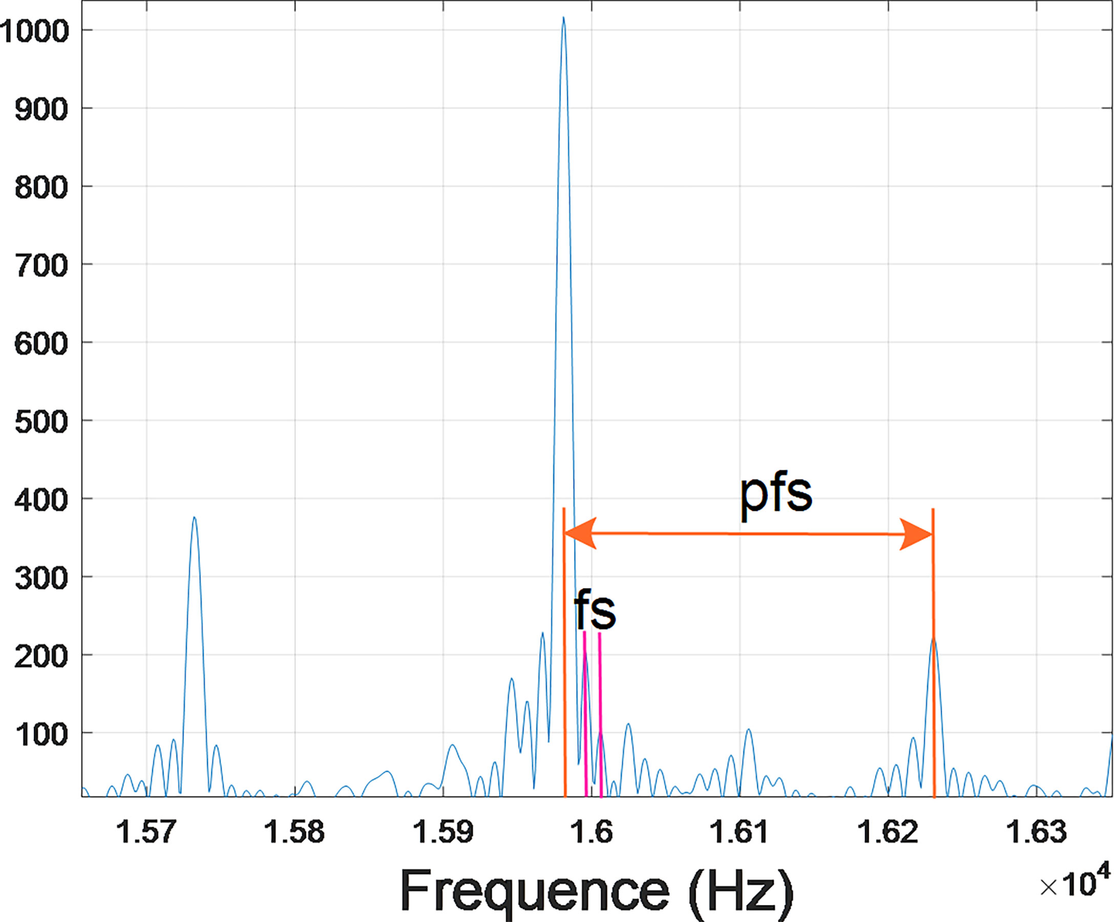
Figure 1 AUV propulsion motor PWM frequency and harmonic frequency.

Figure 1 indicates that a large part of the AUV noise source vibrates below the motor tone. We can determine the PWM switching frequency, PWM, and its multiples. In these propulsion systems, the PWM driving the modulated voltage signal of the BLDC motor is the main noise source. In addition, there are spacing sidebands, f_p and f_s , both around f_PWM . We have experimentally verified that f_p is equal to f_s multiplied by the number of permanent magnet poles, p , in the motor. When the sideband spacing f_s also appears in the motor noise signal, p can be determined.

The AUV is passively tracked by a single element hydrophone. When the AUV is driven by a BLDC motor, we can detect and classify the PWM through its unique high-frequency harmonic acoustic characteristics. Combined with the Doppler signal of PWM generated by AUV movement, the AUV speed can be estimated. Extending these two detection protocols to any AUV scene can realize multi-source tracking and classification.

2.2 Design of AUV detection model for multiple distributed single element hydrophones

In Figure 2, the underwater monitoring network composed of multiple single hydrophones can track AUVs in a large range, thus realizing inexpensive and wide coverage underwater monitoring.

FIGURE 2

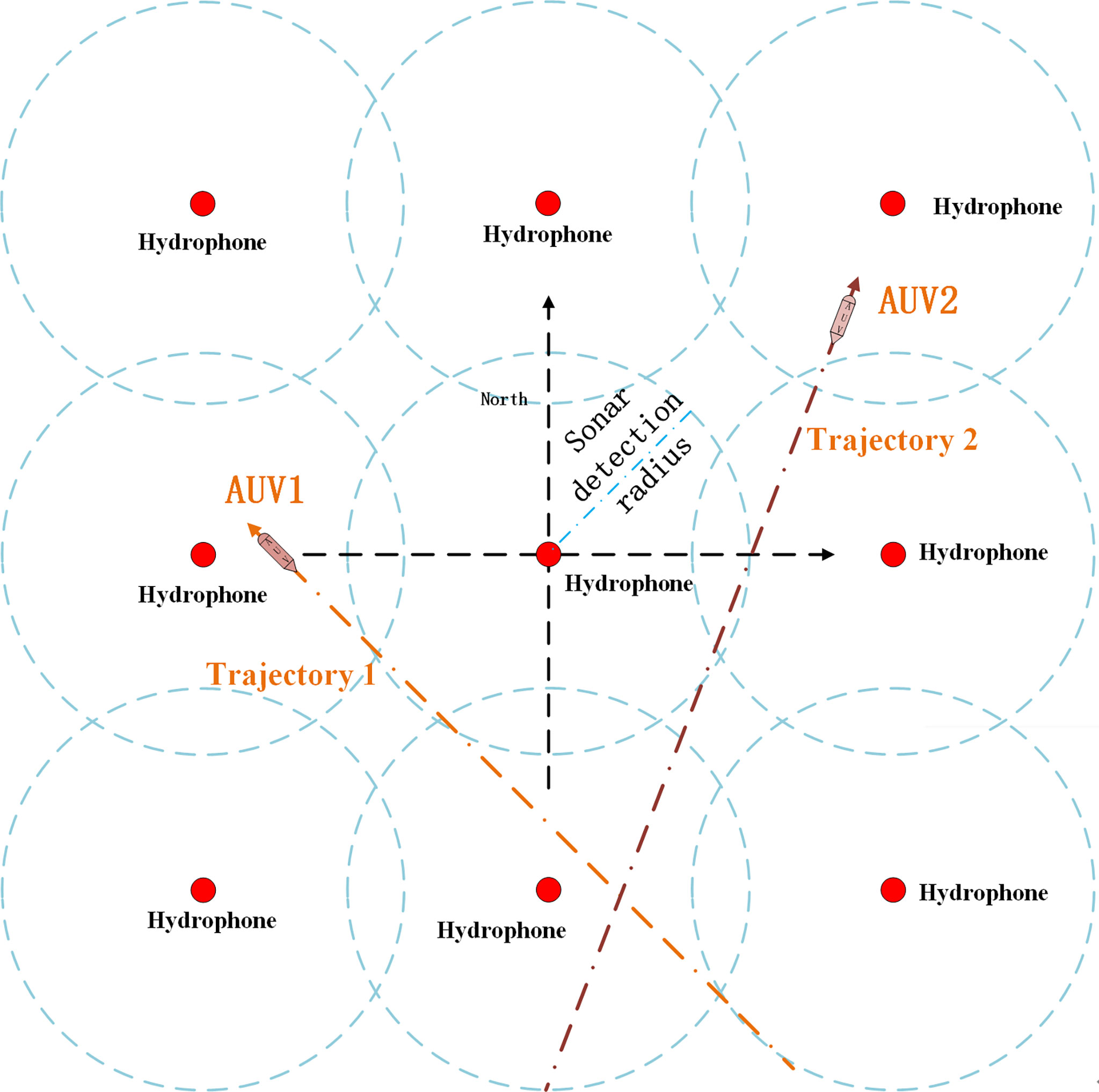
Figure 2 Multiple AUV trajectories and hydrophone position.

A single hydrophone can calculate the AUV velocity and the distance to the hydrophone from the AUV Doppler frequency. Therefore, according to the condition of Assumption 3, monitoring an AUV using two distributed hydrophones will enable the course of the AUV to be estimated from the tangent of the circle formed by the shortest distance between the AUV and the hydrophone. With three hydrophones, it becomes possible to completely determine the route of the AUV, except in one special case. When the AUV course is parallel to the straight line formed by the three hydrophones, only the course can be judged, and two routes will be formed. Figure 3 shows a schematic diagram of the AUV trajectory calculated by the hydrophone network measurement system.

FIGURE 3

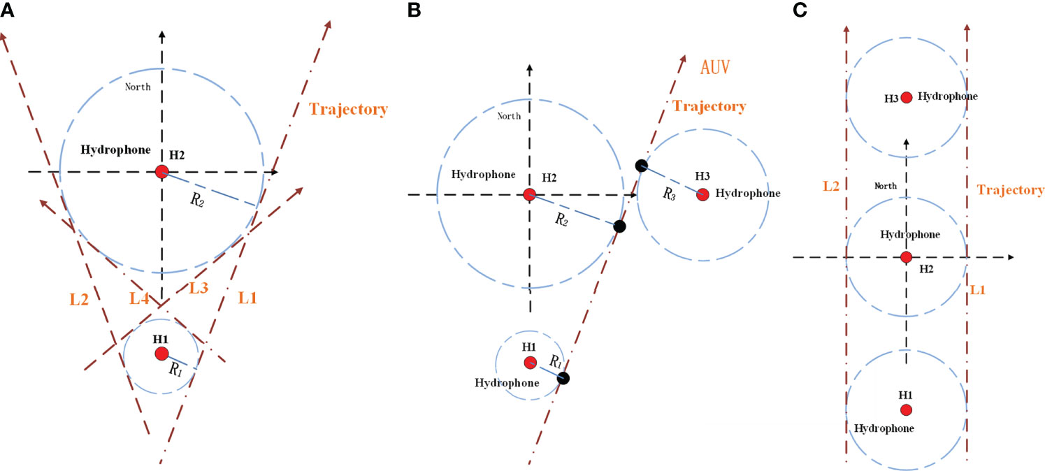
Figure 3 (A) Four possible trajectories of AUV; (B) AUV has only one possible trajectory; (C) Two possible trajectories of AUV.

Lemma 1. According to the common tangent calculation method of (Haiying and Zufeng, 2014), when the position coordinates of R1, R2 which are the yaw distance between the AUV and the hydrophone estimated by the Doppler acoustic signal of the AUV motor of a single hydrophone in Figure 3, and the two hydrophones are known, the parameter equations of the four common tangents L1, L2, L3, and L4 can be obtained. In Figure 3A, L1 and L2 are the outer tangents of two circles, and L3 and L4 are the inner tangents of two circles. The outer tangent length is $l_{\text{out}}=\sqrt{d_{H_1{H}_2}^2-{\left(R_1-R_2\right)}^2}$. The inner tangent length is $l_{inner}=\sqrt{d_{H_1{H}_2}^2-{\left(R_1+R_2\right)}^2}$. According to the time sequence and time difference of the AUV detected and identified by the hydrophone, combined with the velocity of the AUV calculated from the Doppler frequency, the direction of the AUV can be calculated, and two routes can be excluded, that is, L1 and L2 or L3 and L4 are retained. When three hydrophones detect the AUV, the entire AUV trajectory can be calculated, except for the situation shown in Figure 2C.

2.3 Doppler model for single hydrophone detecting multiple AUV motions

According to Assumptions 1–3, the AUV trajectories form straight lines and the velocities remain constant.

The AUV travels in a straight line at a constant speed, and the position of the hydrophone is the coordinate origin. Figure 4 shows the model of a single AUV detected by a single hydrophone. A single hydrophone can only estimate the velocity of the AUV and the yaw position of the shortest-range hydrophone for a linear moving target through the Doppler frequency. The AUV moves in a straight line with a velocity of v_a . Define the vertical distance between the AUV sailing direction and the hydrophone as the yaw distance R_min  between the AUV and the hydrophone, i.e., segment HA3. When displayed in the AUV velocity coordinate system, the AUV Doppler model can be simplified in Figure 4B.

FIGURE 4

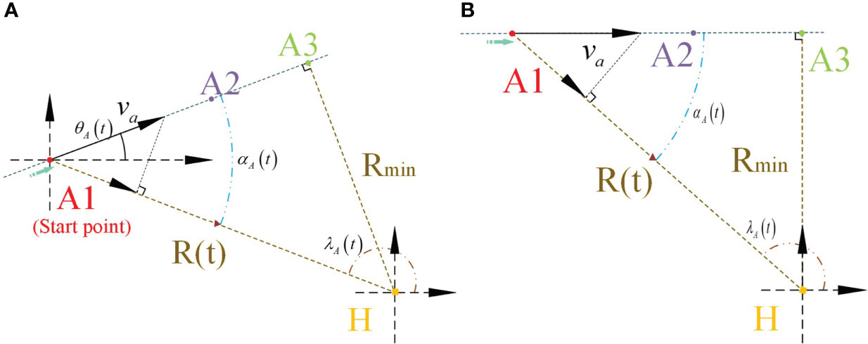
Figure 4 Top view of an AUV’s radiated noise propagation and hydrophone nodes. (A) AUV radiated noise propagation and hydrophone node in Fixed-frame. (B) AUV radiated noise propagation and hydrophone node in AUV velocity frame.

According to Figure 4A, the location of the AUV is (X_A, Y_A) and the location of the hydrophone is (0, 0) with

$\begin{array}{ll}\{\begin{array}{l}{X}_A\left(t\right)=X_A\left(0\right)+v_{A}t\cos {\theta }_A\hfill \\ Y_A\left(t\right)=Y_A\left(0\right)+v_{A}t\sin {\theta }_A\hfill \end{array}& (4)\end{array}$

The AUV velocity v_A is constant and the direction in which the AUV is sailing θ_A is constant. The AUV motion coordinates are (X_A (t), Y_A (t))^T . When the coordinates of the AUVchange with time, the line of sight (LOS) angle of the AUV relative to the hydrophone also changes. The LOS angle is expressed as

$\begin{array}{ll}{\lambda }_A\left(t\right)=\arctan \left(\frac{Y_A\left(t\right)}{X_A\left(t\right)}\right)& (5)\end{array}$

Here, the LOS angle between the AUV and the hydrophone is λ_A (t) . The projection angle α_A of the velocity vector in the LOS direction between the AUV and the hydrophone is

$\begin{array}{ll}\cos {\alpha }_A=\frac{{\overrightarrow{v}}_a·{\left(-X_A\left(t\right),-Y_A\left(t\right)\right)}^T}{\left|{\left(X_A\left(t\right),Y_A\left(t\right)\right)}^T\right|\left|{\overrightarrow{v}}_{ui}\right|}& (6)\end{array}$

In addition, according to the position relationship between the moving sound source and the hydrophone node in the top view shown in Figure 4A, the deflection angle can be determined. When the moving point sound source is on the left or right side of A₁A₂A₃ , the velocity and time are considered to be negative or positive, respectively. The position relationship between the moving point sound source and the stationary node is shown in Figure 4A. Using simple trigonometry, the deflection angle α (t) as a function of time is

$\begin{array}{ll}\alpha \left(t\right)=\arccos \frac{vt}{\sqrt{v^2{t}^2+R_{min }^2}}& (7)\end{array}$

The instantaneous frequency f_d (t) of the AUV sound source received by the hydrophone is

$\begin{array}{ll}{f}_d\left(t\right)=\frac{f_0}{1-\frac{{\overrightarrow{v}}_{a}cos{\alpha }_A}{c_w}}& (8)\end{array}$

where c_w is the underwater sound velocity.

As the AUV moves along a straight line, the sound source deviation angle and LOS angle observed by the hydrophone will change as the relative position between the sound source and the hydrophone varies. In the coordinate system shown in Figure 4, the distance between the sound source and the hydrophone is relatively small, the relative velocity is positive, and the Doppler frequency shift is positive. As the distance between the sound source and the hydrophone increases, the relative velocity and the Doppler shift become negative. When the hydrophone is perpendicular to the course of the AUV, the relative velocity is zero and the Doppler frequency shift is zero. At this time, the distance between the AUV and the hydrophone reaches its minimum.

Figure 5 shows the theoretical values and first and second derivatives of the Doppler frequency shift curve received by the hydrophone before and after a sound source with a resonant frequency of 16 kHz passes through the nearest point (located at a distance of 200 m). The positive and negative values at time t_s cause the asymmetry of the frequency offset. When the AUV is at the same distance from the acoustic receiver h , the frequency offset when it is close to the state is greater than that when it is away from the state.

FIGURE 5

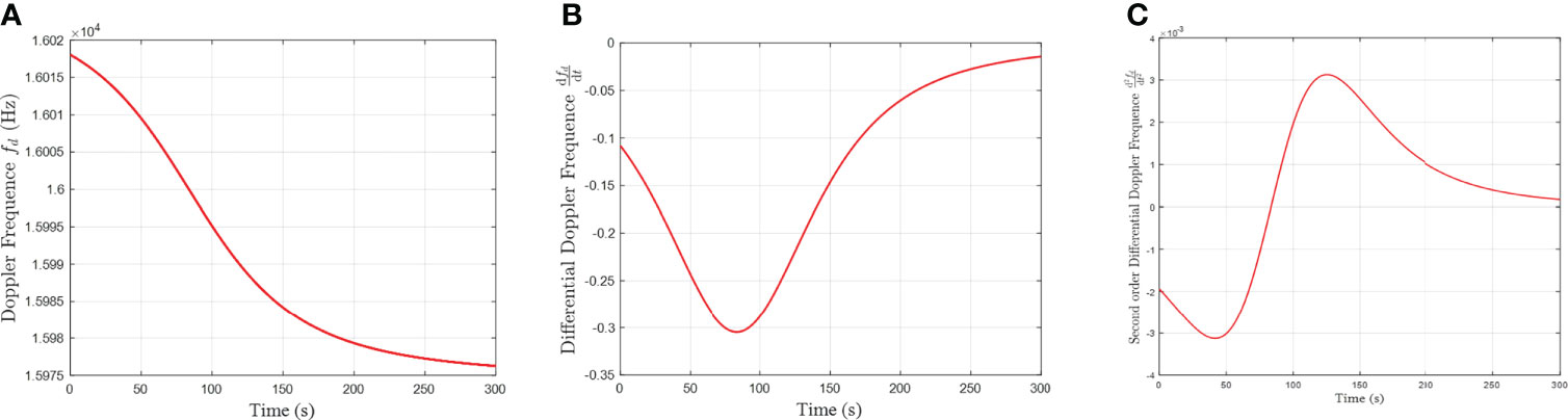
Figure 5 (A) Doppler frequency and its (B) first and (C) second derivatives.

From the relationship between Eq. (4) to Eq. (8), it can be seen that the Doppler frequency shift of the AUV motor underwater acoustic signal is related to the velocity and yaw distance of the AUV. The AUV heading information in Figure 4A cannot be calculated. The actual calculation is completed using the simplified model in Figure 4B.

The natural frequency f₀ and velocity v_A of a point sound source can be calculated from the asymmetry of the curve with respect to time t_s , i.e., positive and negative, and the Doppler frequency shift equation when the sound source is infinite.

$\begin{array}{ll}\{\begin{array}{l}{f}_0=2\frac{f_d\left(-\infty \right)f_d\left(+\infty \right)}{f_d\left(-\infty \right)+f_d\left(+\infty \right)}\hfill \\ v_A=c_w\frac{f_d\left(-\infty \right)-f_d\left(+\infty \right)}{f_d\left(-\infty \right)+f_d\left(+\infty \right)}\hfill \end{array}& (9)\end{array}$

Set the time t = s corresponding to the natural frequency f₀ . Then, the first derivative and the second derivative of the Doppler frequency shift f_d (t) can be calculated, and the time at which the pole value is zero is substituted into

$\begin{array}{ll}\{\begin{array}{l}{\frac{d{f}_d}{dt}|}_{t={\tau }_0}=f_d^{\text{'}}\left({\tau }_0\mid f_0,v,h,w_{\min }\right)\hfill \\ {\frac{d^2{f}_d}{d{t}^2}|}_{t={\tau }_{-1}}=f_d^{\text{'}\text{'}}\left({\tau }_{-1}\mid f_0,v,h,w_{\min }\right)\hfill \end{array}& (10)\end{array}$

Here, τ₀ is the time corresponding to the minimum of $f_d^{"}\left(t\right)$ and τ₋₁ is the time corresponding to the minimum value of $f_d^{"}\left(t\right)$. Thus, the shortest horizontal projection of the point sound source can be obtained. In Eq. (14), the first derivative of the Doppler frequency shift f_d (t) is

$\begin{array}{ll}\frac{d{f}_d}{dt}=-f_0\frac{\frac{{\overrightarrow{v}}_{A}sin{\alpha }_A}{c_w}{\dot{\alpha }}_A}{{\left(1-\frac{{\overrightarrow{v}}_{A}cos{\alpha }_A}{c_w}\right)}^2}& (11)\end{array}$

where c_w is the underwater sound velocity, ${\overrightarrow{v}}_A$ is velocity of AUV.The second derivative of the Doppler shift f_d (t) is

$\begin{array}{ll}\frac{d^2{f}_d}{d{t}^2}=-f_0\left[\frac{c_w{\overrightarrow{v}}_A\left({\ddot{\alpha }}_{A}sin{\alpha }_A+{\dot{\alpha }}_A^{2}cos{\alpha }_A\right)}{{\left(c_w-{\overrightarrow{v}}_{a}cos{\alpha }_A\right)}^2}-2\frac{c_w{\overrightarrow{v}}_A^2\dot{o}t{\alpha }_A^{2}sin{}^2{\alpha }_A}{{\left(c_w-{\overrightarrow{v}}_{A}cos{\alpha }_A\right)}^3}\right]& (12)\end{array}$

3 Multi-frequency estimation design

When a single hydrophone receives navigation noise from multiple AUVs, it can be considered as a multi-component signal. The multi-component signal can be expressed as the linear superposition of multiple single-component signals. By decomposing a multi-component signal into multiple single-component signals, the advantages of the time–frequency method can be effectively used to realize the time–frequency analysis of the multi-component signals. This allows multiple AUVs to be distinguished and the motion parameter information of each AUV to be obtained.

According to the Doppler frequency shift model presented in the previous section and the design principles of AUV motors, combined with Assumptions 1 to 3, when the motor speed of an AUV is constant, Eq. (3) implies that the harmonic frequency difference between f_pwm and f_p is constant. Therefore, an AUV can be identified by a constant frequency difference, and the change trend of the harmonic Doppler frequency of f_pwm and f_p from the same AUV is also consistent. Thus, the Doppler frequency estimation of the harmonics of f_pwm and f_p AUV becomes particularly important.

Multi-component signals are a linear superposition of multiple single-component signals, that is,

$\begin{array}{ll}s\left(t\right)=\sum _{k=1}^N{A}_k\exp \left[j{\varphi }_k\left(t\right)\right]=\sum _{k=1}^N{A}_k\exp \left[j2\pi {\int }^{}\omega \left(t\right)dt\right]& (13)\end{array}$

The multi-component signal can be reduced to the superposition of multiple signals, and each single signal is a variable that needs to be accurately estimated. As the single Doppler signals are time-varying, the dispersed Doppler signal can be represented by an FM signal. According to [34], the FM signal can be expanded as an n -order Taylor series (n ≤ l ) at the point i=0, i.e.,

$\begin{array}{ll}f\left(l\right)=a{e}^{j{\displaystyle \sum _{i=0}^l\omega \left[i\right]}}=a{e}^{j{{\displaystyle \sum _{i=0}^l{\displaystyle \sum _{n=0}^N\frac{{\omega }^{\left(n\right)}\left[0\right]}{n!}\left(\frac{i}{f_s}\right)}}}^n},& (14)\end{array}$

where a∈R⁺ is the amplitude and. is the transient angular frequency. ω⁽ⁿ⁾ [0] is the n -th derivative of ω [i] . As the value of n increases, the signal expanded by this Taylor series becomes closer to the real FM signal. f_s is the sample frequency. The existence of noise has always been considered as a serious effect on the estimation accuracy of IF trajectories. Underwater acoustic noise has an unknown distribution in practical applications, and prior information of the noise distribution is often difficult to obtain. The signal f (l) is corrupted by underwater acoustic noise with an unknown distribution.

3.1 Power of phase-difference accumulation

Sun et al. (2021b) designed a polynomial to approximate the original signal. The IF estimation function obtained by the n -order Taylor series expansion is designed as

$\begin{array}{ll}h\left[i|{\widehat{\omega }}_n\right]=e^{-j{\displaystyle \sum _{i=0}^l{\displaystyle \sum _{n=0}^N\frac{{\widehat{\omega }}^{\left(n\right)}\left[0\right]}{n!}{\left(\frac{i}{f_s}\right)}^n}}}.& (15)\end{array}$

The error between the estimator and the true frequency is

$\begin{array}{ll}r\left[i|{\tilde{\omega }}_u\right]=f\left[i|{\omega }_n\right]h\left[i|{\widehat{\omega }}_n\right]=a{e}^{j{\displaystyle \sum _{i=0}^l{\displaystyle \sum _{n=0}^N\frac{{\widehat{\omega }}^{\left(n\right)}\left[0\right]}{n!}{\left(\frac{i}{f_s}\right)}^n}}},& (16)\end{array}$

where ${\tilde{\omega }}_u={\omega }_u-{\widehat{\omega }}_u$ is the frequency expansion error and $\varphi \left[i|{\tilde{\omega }}_u\right]=\sum _{n=0}^N\frac{{\tilde{\omega }}^{\left(n\right)}\left[0\right]}{n!}{\left(\frac{i}{f_s}\right)}^n$ is the phase error. When the phase error $\varphi \left[i|{\tilde{\omega }}_u\right]=0$, the FM signal frequency is ${\widehat{\omega }}_u={\omega }_u$.

The coherent accumulation of phase difference can improve the signal-to-noise ratio (SNR) (Du et al., 2020). For underwater acoustic noise with an arbitrary distribution, the average value of coherence accumulation will fluctuate slightly; however, the coherence accumulation of phase difference in Eq. (16) will increase with time, especially when $\varphi \left[i|{\tilde{\omega }}_u\right]$ is approximately zero [42]. Inspired by this fundamental rule, a cost function is constructed to find the optimal solution for all coefficients $\varphi \left[i|{\tilde{\omega }}_u\right]$:

$\begin{array}{ll}p\left[l|{\tilde{\omega }}_u\right]=\frac{1}{l}\sum _{i=0}^l\left\{\sum _{k=0}^{i}r\left[k|{\tilde{\omega }}_u\right]-r_m\left[i|{\tilde{\omega }}_u\right]\right\}\left\{\sum _{k=0}^{i}r\left[k|{\tilde{\omega }}_u\right]-r_m\left[i|{\tilde{\omega }}_u\right]\right\}*& (17)\end{array}$

with $r_m\left[i|{\tilde{\omega }}_u\right]=\frac{1}{i}\sum _{k=0}^{i}r\left[k|{\tilde{\omega }}_u\right]$. In the above cost function, $\sum _{k=0}^{i}r\left[k|{\tilde{a}}_u\right]$ is the sum of the accumulated phase difference of i points in $r\left[k|{\tilde{\omega }}_u\right]$ and * denotes the complex conjugate. The power $p[l|{\tilde{\omega }}_{u}ght]$ and its mean value over the period l improve the anti-interference ability of the spectrum to a certain extent.

Lemma 2. The cumulative phase difference power $p\left[l|{\tilde{\omega }}_u\right]$ minus the mean is a monotonically decreasing function of the coefficient modulus $\left|{\tilde{\omega }}_u\right|$ (Sun et al., 2021b; Sun et al., 2021a).

3.2 Instantaneous frequency estimation based on nonlinear accumulated phase power logarithm

In view of the nonlinear amplification for DOA estimation and IF estimation described by Filippini et al. (2019); Sun et al. (2021b), and Zhang et al. (2018), a multiple logarithmic sum is proposed to achieve a sharper peak for the true IF and a deeper trough for the area that is not of interest. This will also improve the accuracy and robustness of the IF estimation. On this basis, a log-sum-multiple function is used for the maximization, as this is more convex and smoother than a log-sum. This function also exhibits nonlinear amplification in some fixed intervals.

$\begin{array}{ll}\begin{array}{l}\underset{{\widehat{p}}_u}{\max }{J}_1\left({\tilde{\omega }}_u\right)=\log \frac{{\prod }_{l=0}^{L-1}\left\{p\left[l|{\tilde{\omega }}_u\right]+1\right\}}{{\sum }_{l=0}^{L-1}t\{p\left[l|{\tilde{\omega }}_u\right]+1}\hfill \end{array}=\sum _{l=0}^{L-1}\log \left\{p\left[l|{\tilde{\omega }}_u\right]+1\right\}-\log \sum _{l=0}^{L-1}\left\{p\left[l|{\tilde{\omega }}_u\right]+1\right\}\text{s}.\text{t}.{\tilde{\omega }}_u={\omega }_u-{\widehat{\omega }}_u& (18)\end{array}$

where “1” is introduced into the integrand to ensure a simple analytical solution.

Under the condition of short-time window function or strong noise, the L1 norm method has poor estimation accuracy or is susceptible to noise interference. The log product sum ratio is used to increase the peak value of the target instantaneous frequency in the time spectrum and suppress the side lobe of the non target region. Under the condition of small sample data or low signal-to-noise ratio, this method can effectively improve the accuracy and stability of the time-frequency estimation curve.

Remark 2. Eq. (18) can be understood as the logarithmic mapping of the cumulative power at each time minus the logarithmic mapping of the cumulative power at all times.

The lower limit of $J_1\left({\tilde{\omega }}_u\right)$ is

$\begin{array}{ll}\underset{{\tilde{p}}_u\to -\infty }{\lim }\{\sum _{l=0}^{L-1}\log \left\{p\left[l|{\tilde{\omega }}_u\right]+1\right\}-\log \sum _{l=0}^{L-1}\text{ {}p[lt\mid {\tilde{\omega }}_u\text{] }+1\}=0& (19)\end{array}$

If the upper limit of $J_1\left({\tilde{\omega }}_u\right)$ is a variable $v\left({\tilde{\omega }}_u\right)$, the variable upper limit integral of $J_1\left({\tilde{\omega }}_u\right)$ can be expressed as

$\begin{array}{ll}{J}_2\left[v\left({\tilde{\omega }}_u\right)\right]=\underset{1}{\overset{v\left({\tilde{\omega }}_u\right)}{\int }}\left(\log \kappa +1\right)d\kappa =v\left({\tilde{\omega }}_u\right)\log v\left({\tilde{\omega }}_u\right)& (20)\end{array}$

where “1” is introduced into the integrand to ensure a simple analytical solution. Sun et al., 2021a showed that $J_2\left[\nu \left({\tilde{p}}_u\right)\right]$ is a convex function about $\nu \left({\tilde{p}}_u\right)$.

Lemma 3. $J_2\left({\tilde{\omega }}_u\right)$ is a convex function (Boyd et al. (2004)).

Theorem 1. $J_2\left({\tilde{\omega }}_u\right)$ is a monotonically decreasing function of ${\tilde{\omega }}_u$. According to the chain rule, the first derivative of $J_2\left[\nu \left({\tilde{\omega }}_u\right)\right]$ with respect to $\left|{\tilde{\omega }}_u\right|$ is

$\begin{array}{ll}\frac{d{J}_2\left[v\left({\tilde{p}}_u\right)\right]}{d\left|{\tilde{\omega }}_u\right|}=\frac{d{J}_2}{d\nu }\sum _{l=0}^{L-1}\left(\frac{d\nu }{dp\left[l\right]}\frac{dp[l\text{ ∣ }{\tilde{\omega }}_{u}right.]}{d\left|{\tilde{\omega }}_u\right|}\right)& (21)\end{array}$

To determine whether Eq. (21) is positive or negative, we analyze the positive and negative nature of the first-order functions $\frac{d{J}_2}{dv}$, $\frac{dv}{dp\left[l\right]}$, and $\frac{dp\left[l|{\tilde{\omega }}_u\right]}{d\left|{\tilde{\omega }}_u\right|}$.

According to Lemma 1, $p\left[l|{\tilde{\omega }}_u\right]$ is a monotonically decreasing function of $\left|{\tilde{\omega }}_u\right|$ and $\frac{dp\left[l|{\tilde{\omega }}_u\right]}{d\left|\tilde{o}meg{a}_u\right|}\le 0$. Then, in Eq. (20), $\nu \left\{p\left[l\right]\right\}=\frac{{\prod }_{l=0}^{L-1}\left\{p\left[l|{\tilde{\omega }}_u\right]+1\right\}}{{\sum }_{l=0}^{L-1}\left\{p\left[l|\stackrel{⌢}{ı}lde{\omega }_u\right]+1\right\}}$, $\frac{dv}{dp\left[l\right]}$ can be expressed as

$\begin{array}{ll}\frac{dv\left\{p\left[l\right]\right\}}{dp\left[l\right]}={\left(\frac{{\prod }_{l=0}^{L-1}\left\{p\left[l\mid {\tilde{\omega }}_u\right]+1\right\}}{{\sum }_{l=0}^{L-1}\left\{p\left[l\mid {\tilde{\omega }}_u\right]+1\right\}}\right)}_{p[[]}=\frac{{\left({\prod }_{i=0}^{L-1}\left\{p\left[l\mid lde{\omega }_u\right]+1\right\}\right)}_{p\left[l\right]}}{{\sum }_{l=0}^{L-1}\left\{p\left[l\mid {\tilde{\omega }}_u\right]+1\right\}}-\frac{{\prod }_{l=0}^{L-1}\left\{p\left[l\mid {\tilde{\omega }}_u\right]+1\right\}}{{\left({\sum }_{l=0}^{L-1}\left\{p\left[l\mid {\tilde{\omega }}_u\right]+1\right\}\right)}^2}(\sum _{l=0}^{L-1}\left\{p\left[l\mid {\tilde{\omega }}_u\right]+1\right\}t{)}_{p\left[l\right]}=\frac{{\prod }_L\left\{p\left[k\mid {\tilde{\omega }}_u\right]+1\right\}}{{\sum }_{l=0}^{L-1}\left\{p\left[l\mid {\tilde{\omega }}_u\right]+1\right\}}-\frac{{\prod }_{l=0}^{L-1}\left\{p\left[l\mid {\tilde{\omega }}_u\right]+1\right\}}{{\left({\sum }_{l=0}^{L-1}\left\{p\left[l\mid {\tilde{\omega }}_u\right]+1\right\}\right)}^2}L& (22)\end{array}$

where k∈ {0, L − 1} ∖ {l} . In Eq. (22), because the power $p\left[l|{\tilde{\omega }}_u\right]\ge 0$, we have that $\frac{L}{{\sum }_{l=0}^{L-1}\left\{p\left[l|{\tilde{\omega }}_u\right]+1\right\}}\le 1$ and $\frac{dv\left\{p\left[l\right]\right\}}{dp\left[l\right]}\ge 0$. v {p [l]} is a monotonically increasing function of p [l | deω_u] .

Finally, the first derivative of $J_2\left[\nu \left({\tilde{\omega }}_u\right)\right]$ with respect to $\nu \left({\tilde{\omega }}_u\right)$ is

$\begin{array}{ll}\frac{d{J}_2\left[v\left({\tilde{\omega }}_u\right)\right]}{dv}=\log \nu \left({\tilde{\omega }}_u\right)+1& (23)\end{array}$

Because $\nu \left({\tilde{\omega }}_u\right)\ge 1$, Eq. (23) is positive. $J_2\left[\nu \left({\tilde{\omega }}_u\right)\right]$ is a monotonically increasing function of $\nu \left({\tilde{\omega }}_u\right)$. In summary, the first derivative of $J_2\left[\nu \left({\tilde{\omega }}_u\right)\right]$ with respect to $\left|{\tilde{\omega }}_u\right|$ is non-positive:

$\begin{array}{ll}\frac{d{J}_2\left[\nu \left({\tilde{\omega }}_u\right)\right]}{d\left|{\tilde{\omega }}_u\right|}\le 0& (24)\end{array}$

Therefore, $J_2\left[\nu \left({\tilde{\omega }}_u\right)\right]$ is a monotonically decreasing function of $\left|{\tilde{\omega }}_u\right|$.

The estimation coefficient $\widehat{\omega }$ can be obtained by solving the following optimization problem:

$\begin{array}{ll}\underset{{\widehat{\omega }}_u}{\max }{J}_2\left({\tilde{\omega }}_u\right)=\nu \left({\tilde{\omega }}_u\right)\log \nu \left({\tilde{\omega }}_u\right)\text{ s}.\text{t}.{\tilde{\omega }}_u={\omega }_u-\widehat{e}g{a}_u& (25)\end{array}$

When ${\widehat{\omega }}_u$ is known, the estimated IF can be obtained as $\widehat{\varphi }\left[i|{\widehat{\omega }}_u\right]=\sum _{u=0}^U{\widehat{\omega }}_u{\left(\frac{i}{f_s}\right)}^u$. According to Theorem 1, $J_2łeft({\tilde{\omega }}_u)$ is a convex function, so the optimal value can be determined using a gradient method.

The algorithm based on the log-sum multiple function has the characteristics of a deep zero sidelobe and extremely sharp main lobe. In Figure 6, compared with the APP-MLS algorithm (Sun et al., 2021b), the proposed algorithm gives a lower main lobe value than the APP-MLS algorithm. This reduces the computational complexity and hardware requirements caused by possible large data values in the calculation. At the same time, because PAL-PSR algorithm has sufficiently high IF resolution, there is no side sidelobe leakage of Fourier transform in Figure 6.

FIGURE 6

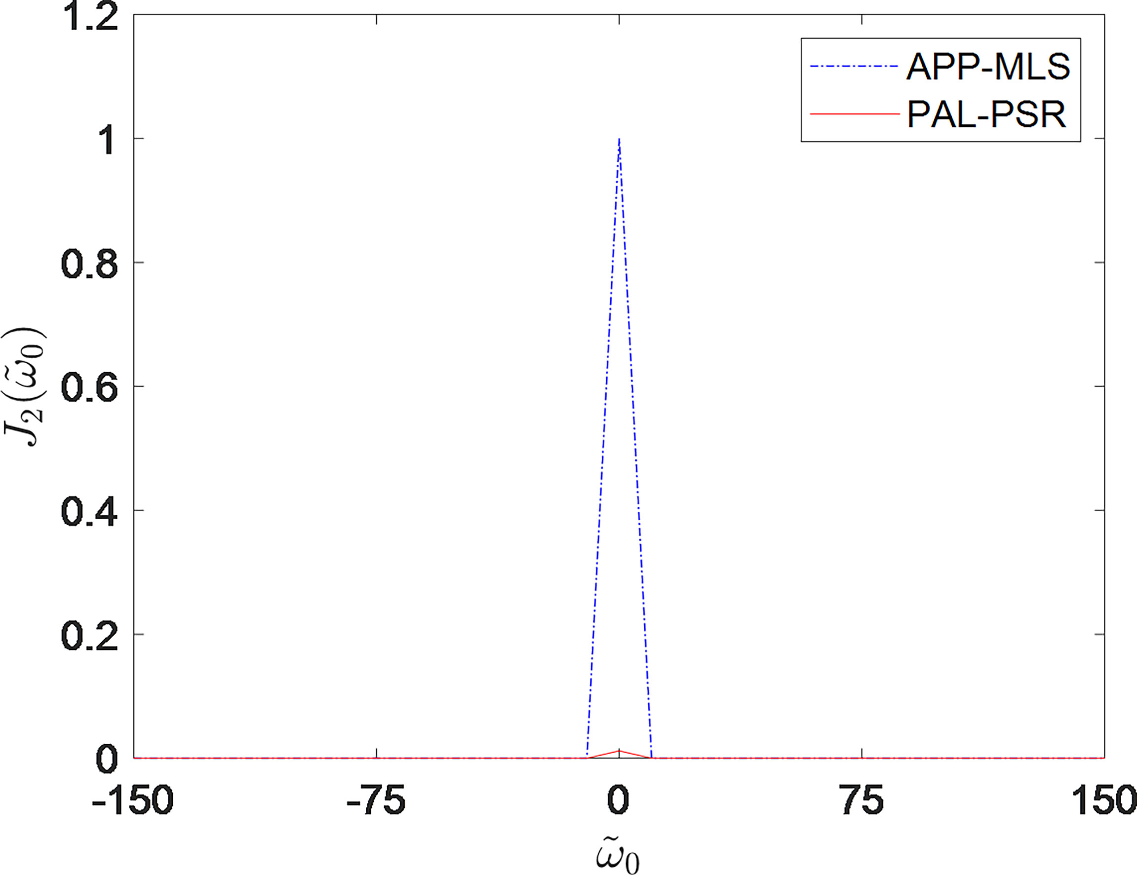
Figure 6 $J_2\left({\tilde{\omega }}_u\right)$ comparison between PAL-PSR and APP-MLS.

In the process of using this algorithm, the estimation accuracy of the time–frequency curve will be affected by the order U , the length of the rectangular window W , and the sliding length L . Specifically, if the length of the rectangular window W is constant, an increase in the order U means that the fitting polynomial function will provide a better approximation to the real frequency function. Thus, the final estimated time–frequency φ [m] will be of higher accuracy. If the order is fixed, an increase in the length of the rectangular window W will increase the error between the fitting polynomial function and the real frequency function as the number of sample points increases, so the accuracy of the final time–frequency curve will become worse. The error will be greatest at the last point in the window. However, W also determines the stability of the algorithm. A longer window length produces a stronger ability to suppress different distributed noise. Therefore, the value of W should not be too small in practical applications. A longer sliding length L gives a larger deviation between the estimated IF time–frequency φ [m] and the actual curve. In addition, larger values of the order U , rectangular window length W , and sliding length L will increase the computational complexity of the algorithm. In practice, appropriate parameter values should be selected according to accuracy, stability, and computational complexity requirements.

3.3 Multi-AUV frequency identification

In Figure 6, the PAL-PSR algorithm produces a sharper peak and lower sidelobe region, so it can accurately distinguish multiple frequencies.

$\begin{array}{ll}{\widehat{\omega }}_i\left(t\right)-{\widehat{\omega }}_j\left(t\right)=a& (26)\end{array}$

where a is a constant and i , j are nonadjacent spectral lines. According to Eq. (3), such a set of constant frequencies can be considered as the PWM frequency of a BLDC motor, propeller modulation frequency, and electrode modulation frequencyfrom the same AUV.

When a single hydrophone receives AUV motor noise, if the motor frequency f_pwm used by the AUV is the same or close, some frequency crossover will occur after time–frequency estimation of multiple frequency bands, as shown in Eq. (3).

The energy of the same frequency signal increases at the frequency intersection, so it can be judged that the frequency has crossed over. The crossover frequency is used as the Doppler information of the motion of two AUVs at the same time, combined with the first-order derivatives f_pwm and f_p and the second-order derivatives f_pwm and f_p of AUV motion. This modulation signal assists in distinguishing AUV motion information.

According to the above analysis, this paper proposes an AUV signal detection algorithm. The specific steps are as follows:

Step 1: Calculate the STFT of the signal and judge the signal interval according to the stable energy value of the STFT in the frequency domain. Specifically, search for a stable value that exceeds the threshold in the frequency domain within each time window. According to the theory of signal detection and estimation, for a given false alarm probability, it is difficult to give an accurate detection threshold. In practice, the detection threshold is generally determined by the method of numerical statistics (Li et al., 2011; Zhu et al., 2021). According to whether the selected amplitude frequency continuously exceeds the threshold in continuous time, the false alarm probability can then be reduced.

Step 2: Among the frequencies screened in step 1, the PAL-PSR algorithm is used for frequency estimation. The peak of the deep zero sidelobe is then formed after accurate frequency estimation, allowing the frequencies that the STFT algorithm cannot distinguish to be identified.

Step 3: Multiple AUVs are distinguished according to the frequency estimated in step 2, combined with the BLDC frequency characteristics of the AUVs and the Doppler frequency shift.

Remark 3. According to Eq. (8), if the speed difference of multiple AUVs equipped with similar BLDC motors is large, the modulation frequency generated by f_p at f_pwm will be relatively different, and the frequency may not crossover. When the sailing speeds are similar, the modulation frequency generated by f_p at f_pwm may also cross frequency. When frequency crossover occurs, as shown in Eq. (9), the Doppler frequency is a continuous differentiable function. Thus, different AUVs can be distinguished and AUV motion information can be extracted by judging the continuity of f_pwm and the fixed frequency difference between f_pwm and the harmonic signal.

4 Simulations

This section compares the performance of the PAL-PSR algorithm with several classical IF estimation algorithms, including the STFT, WVD, polynomial chirplet transform, and synchrosqueezing transform (SST). The algorithms are assessed using a sinusoidal FM signal (SFM). The sample time is T = 1 s and the sample frequency is f_s = 50 kHz. In Figure 7A, B, the window size W and the overlap size S are set to 200 and 20, respectively, considering the tradeoff between computation time and the ability to suppress noise. Symmetric α -stable (SaS) noise (Zhang et al., 2022) is often used to model underwater acoustic noise, as it represents real-world noise with changing statistical characteristics (Jobst et al., 2020). The generalized SNR (GSNR) (Ferrari et al., 2020) isused, which is defined as the ratio of the signal’s average power to the noise dispersion in the finite interval of interest:

$\begin{array}{ll}\text{GSNR }=10\underset{10}{\log }\frac{a^2}{\gamma }& (27)\end{array}$

FIGURE 7

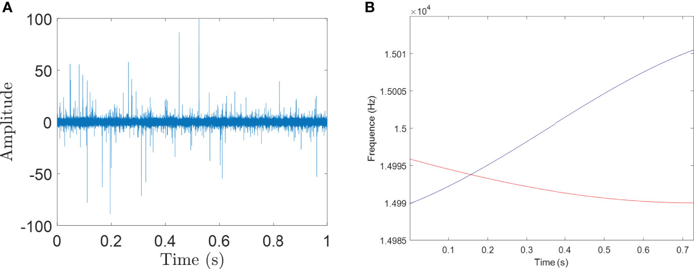
Figure 7 (A) SFM signal with noise, (B) designed frequency curve of cross SFM signal.

An SFM signal is often used as the detection signal for sonar and radar because it offers increased bandwidth and can maintain a large pulse interval:

$\begin{array}{ll}{x}_{GSFM}\left[l\right]=e^{i{\displaystyle \sum _{m=0}^l{\phi }_{SFM}\left[m\right]}},& (28)\end{array}$

where the IF is set to

$\begin{array}{ll}{\phi }_{SFM}\left[m\right]=15000+10.*\text{ cos }\left(a2\pi m+a2\pi \right)& (29)\end{array}$

Although most noise can be assumed to follow a Gaussian distribution, there exist other types of underwater acoustic noise with unknown distributions, and prior information of the noise distribution is often difficult to obtain. SaS noise has been used to model various types of real underwater acoustic noise (Gogineni et al., 2020; Zhang et al., 2021). Under the condition of a heavy tailing effect, that is, adding SaS noise with a characteristic index of α = 1.6 to the signal, and setting GSNR=−10dB , we compare the performance of the proposed time–frequency estimation algorithm with four classical methods. In the simulations, we set the window length W = 200 and sliding length L = 50 . The SFM signal polluted by strong noise is shown in Figure 11A.

Figure 8 shows the estimation results of STFT, WVD, and SST. Due to the intersection of signal frequencies, the energy aggregation of the time–frequency estimation curves is scattered, and the STFT is more vulnerable to noise interference, resulting in a fuzzy time–frequency distribution. Figure 8B shows that WVD is highly ambiguous around the signal frequency intersection. Figure 8C shows the results given by the SST. The large number of pulses distorts the time–frequency trajectories to varying degrees, making it difficult to suppress high-energy noise. As can be seen from Figure 8D, compared with the four existing methods, the proposed time–frequency estimation algorithm not only maintains high energy aggregation, but also obtains high time–frequency trajectories, which verifies the accuracy and stability of our approach. Figure 8E shows the relative errors of the five time–frequency estimation curves. The error results show that the proposed time–frequency estimation algorithm effectively suppresses high-energy noise.

FIGURE 8

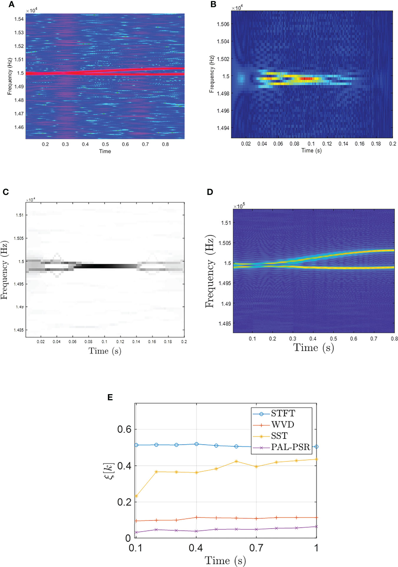
Figure 8 (A) STFT curve of cross SFM signal, (B) WVD curve of cross SFM signal, (C) SST curve of cross SFM signal, (D) PAL- PSR curve of cross SFM signal, (E) eelative error curves for STFT, WVD, SST, and PAL-PSR. GSNR2=-10 dB.

5 Experiments

5.1 Experiments

According to Coraluppi et al. (2018) and Zhu et al. (2021), the thruster operates at a fixed PWM frequency of 15–20 kHz, and it has been verified that there is a strong signal at the PWM frequency of the motor. An experiment was carried out using an electrically propelled unmanned surface vessel (USV). During the movement of the USV, a strong single-frequency signal at the PWM frequency of the USV propeller motor can be observed in the hydrophone measurement data (Figures 9A, B). When the propeller state remains unchanged, the PWM frequency will not vary. According to the conditions specified in Assumption 1 to Assumption 3, the USV was set to sail in a straight line at a uniform speed in the due north direction.

FIGURE 9

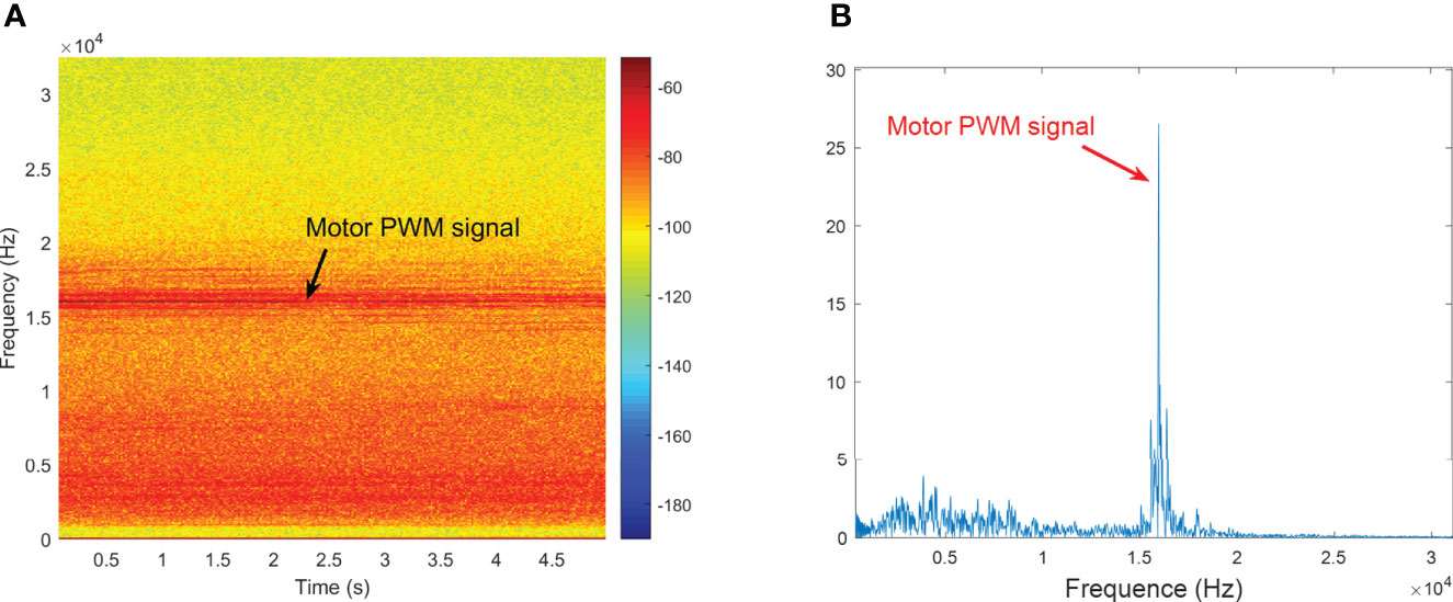
Figure 9 (A) Time–frequency diagram of USV motor, (B) frequency diagram of USV motor.

Experiments were carried out on a lake, with the position of the hydrophone taken as the coordinate origin. The hydrophone was fixed at a depth of 0.5 m. Two ships with the same motor were used to conduct experiments, and the data obtained from the motor acoustic signals of the two ships were processed.

In the experiment, f_pwm = 16005 Hz under the static condition of the USVs. The USVs move according to Assumption 1 to Assumption 3. USV1 has a velocity of 2.9 m/s and USV2 has a velocity of 3.8 m/s. The USVs sail in a straight line. Figures 19–21 compare the estimated time–frequency curves of the hydrophone after receiving the experimental data through PAL-PSR and the Doppler time–frequency curve calculated according to the coordinates of the USV positions and the receiving hydrophone. According to the motion parameters of the USVs calculated from the time–frequency curve, combined with Assumptions 1–3, the estimated navigation parameters of the USVs were obtained. When the Doppler frequency of USV motion is used in Eq. (8), it is possible to solve Eq. (8). The movement time of the USVs is 15 s. Through comparative experiments, the maximum deviation between f_pwm measured at rest and f_pwm obtained by calculating the derivative of the Doppler signal of the USVs is 0.8 Hz. The deviation in f_p is 0.9 Hz. The results of the lake experiment are presented in Table 1. The relative error between the USV and hydrophone positions retrieved by Eq. (8) and the GPS locations is not more than 7%, and the USV velocity estimation error is not more than 4%.

TABLE 1

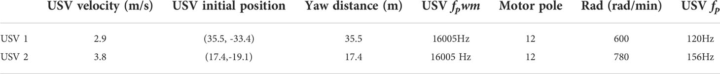
Table 1 USV navigation conditions.

Comparing the transformation results of the experimental data by the two algorithms in Figures 10B, C, it can be seen that the spectrum obtained by the STFT in Figure10A has obvious frequency broadening, and it is unable to accurately judge the frequency intersection generated by multiple AUVs, and it is unable to accurately estimate the frequency. Only the trend of frequency transformation can be roughly seen. However, STFT can determine the approximate frequency range, and then use PAL-PSR algorithm to accurately estimate the frequency and distinguish the targets.

FIGURE 10

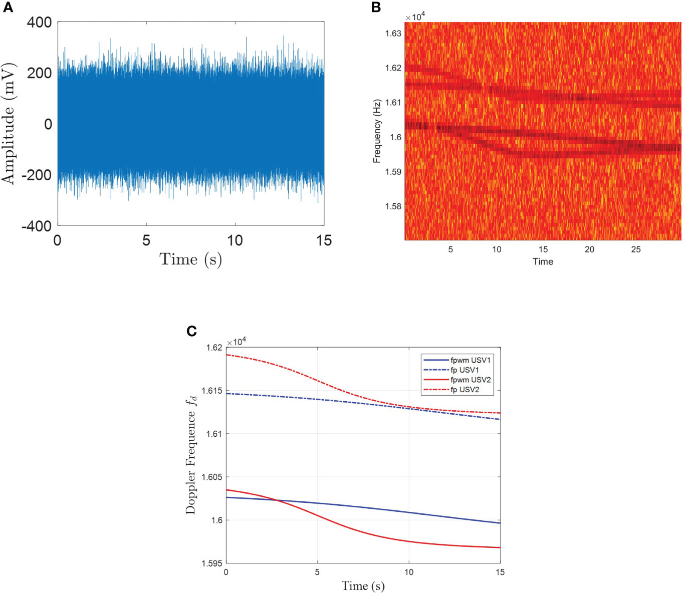
Figure 10 (A) Time-domain signal collected by the hydrophone in the experiment, (B) STFT curve of f_pwm and f_p in the experiment, (C) PAL-PSR curve of f_pwm and f_p in the experiment.

From Figure 10C, combined with the Doppler frequency of Eq. (8) and the motor modulation frequency in Eq. (3), when the sailing velocity of the USVs is different, the motor speeds are also different. Thus, the position where the frequency crossover occurs will change. However, because f_p is modulated in f_pwm , the frequency difference between f_pwm and f_p remains unchanged, as shown in Eq. (26).

The first and second derivatives of f_pwm for the different USVs are shown in Figures 11A, B. According to Eq. (7) and Eq. (8), the minimum value of the first derivative and the zero value of the second derivative indicate the shortest distance between the USV and the hydrophone, that is, the yaw position. According to the time at which the yaw position occurs, the USV velocity, f_pwm , f_p , and yaw distance of the USV can be calculated.

FIGURE 11

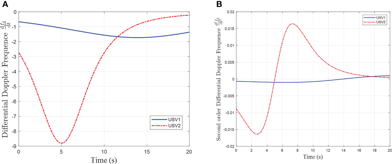
Figure 11 (A) First-order derivative of the estimated frequency f_pwm, (B) second-order derivative of the estimated frequency f_pwm..

5.2 Experimental data error analysis

During the experiment, there was a deviation between the GPS locations and measured Doppler signal, as shown in Table 1. The algorithm was used to estimate the motion state parameters of the USV. The estimated results and errors are shown in Table 2. In the estimation process, external interference, including measurement errors associated with GPS and the USV inertial navigation system, created some deviation between the propeller and GPS measurement points, resulting in errors in the nonlinear calculation process. In the experiment, the hydrophone monitored the PWM signal of the propulsion motor. The distance between the propulsion motor and the GPS/INS position was 2.5 m. In addition, due to the influence of noise, the estimated Doppler frequency shift will have some degree of error. Thus, using only the starting time and the shortest distance time to estimate the yaw position and navigation speed of the USV will introduce a certain deviation. If multiple points were used as the start time (e.g., 0.5 s, 1 s) and the shortest distance time, and the data were averaged to reduce the error, the results presented in Table 3 would be obtained.

TABLE 2

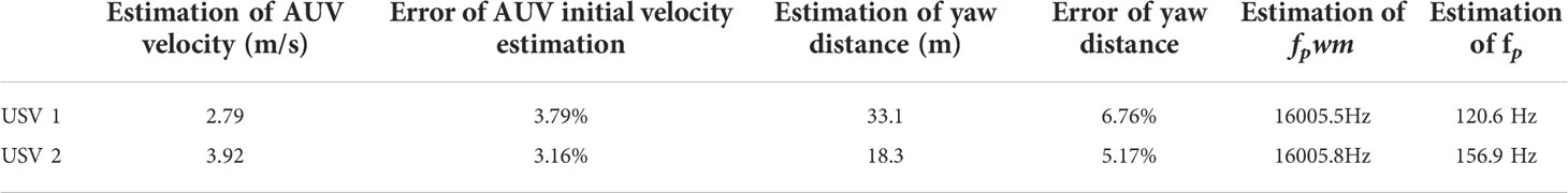
Table 2 Inversion calculation of USV circle navigation conditions and errors.

TABLE 3

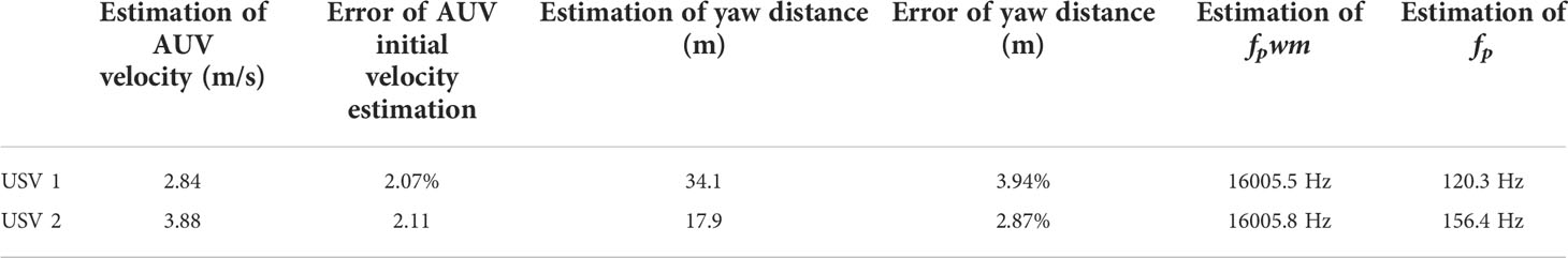
Table 3 Motion trajectory at multiple times after initial calculation time.

6 Conclusion

In this paper, we investigated the signal characteristics of AUV propulsion motors and designed a multi-AUV linear motion model. According to the motion model and the Doppler information generated by the motor signal, the relative position between the AUV and a hydrophone was calculated. The proposed PAL-PSR algorithm can accurately estimate the underwater acoustic frequency curve, even in the presence of impulse signal noise. As the cost function is a monotonic function of frequency, the estimation result is stable. Accurate estimations are possible because the nonlinear amplification mapping allows the signal to grow exponentially in energy, whereas the noise grows linearly at most. Through computer simulations, the effectiveness of the PAL-PSR method was verified under different GSNRs and window sizes. Compared with some classical methods, PAL-PSR exhibits excellent performance and robustness in the presence of an unknown noise distribution. In addition, by examining the characteristics of AUV motors, an AUV judgment mechanism based on the PAL-PSR frequency estimation method was designed, enabling a single hydrophone to distinguish multiple AUVs through their signal characteristics. A lake experiment was conducted using USVs and a single hydrophone. The PAL-PSR algorithm was used to estimate the FM signal curve received by a single hydrophone. According to the frequency modulation curve, the positions of the USVs were retrieved and compared with the ground-truth GPS coordinate positions.

Data availability statement

The original contributions presented in the study are included in the article/supplementary material. Further inquiries can be directed to the corresponding author.

Author contributions

SR: Conceptualization, Methodology, Software, Writing - Original Draft. YX: Writing - Review and Editing, Supervision, Software, Funding acquisition, Project administration. All authors contributed to the article and approved the submitted version.

Funding

This research was supported by Zhejiang Provincial Natural Science Foundation of China under Grant No.LY21F010001.

Conflict of interest

The authors declare that the research was conducted in the absence of any commercial or financial relationships that could be construed as a potential conflict of interest.

Publisher’s note

All claims expressed in this article are solely those of the authors and do not necessarily represent those of their affiliated organizations, or those of the publisher, the editors and the reviewers. Any product that may be evaluated in this article, or claim that may be made by its manufacturer, is not guaranteed or endorsed by the publisher.

References

Acarnley P. P., Watson J. F. (2006). Review of position-sensorless operation of brushless permanent-magnet machines. IEEE Trans. Ind. Electron. 53, 352–362. doi: 10.1109/TIE.2006.870868

CrossRef Full Text | Google Scholar

Boyd S., Boyd S. P., Vandenberghe L. (2004). Convex optimization (Cambridge:Cambridge University Press, British).

Google Scholar

Brinkmann K., Hurka J. (2009). “Broadband passive sonar tracking,” in Informatik 2009–im focus das leben (Germany:Gesellschaft f{\"u}r Informatik e. V).

Google Scholar

Buckingham M. J., Giddens E. M., Simonet F., Hahn T. R. (2002). Propeller noise from a light aircraft for low-frequency measurements of the speed of sound in a marine sediment. J. Comput. Acoust. 10, 445–464. doi: 10.1142/S0218396X02001760

CrossRef Full Text | Google Scholar

Coraluppi S., Carthel C., Coon A. (2018). “An MHT approach to multi-sensor passive sonar tracking,” In 2018 21st International Conference on Information Fusion (FUSION). (Cambridge, UK:IEEE) 480–487.

Google Scholar

De Viaene J., Verbelen F., Derammelaere S., Stockman K. (2018). Energy-efficient sensorless load angle control of a BLDC motor using sinusoidal currents. IET Electr. Power Appl. 12, 1378–1389. doi: 10.1049/iet-epa.2018.5059

CrossRef Full Text | Google Scholar

Du S., Zhang J., Hu G. (2020). A robust data-driven AVO inversion with logarithm absolute error loss function. Acta Geophy. 68, 445–458. doi: 10.1007/s11600-020-00416-1

CrossRef Full Text | Google Scholar

Fang J., Wang F., Shen Y., Li H., Blum R. S. (2016). Super-resolution compressed sensing for line spectral estimation: An iterative reweighted approach. IEEE Trans. Signal Process. 64, 4649–4662. doi: 10.1109/TSP.2016.2572041

CrossRef Full Text | Google Scholar

Ferguson B. G. (1992). A ground-based narrow-band passive acoustic technique for estimating the altitude and speed of a propeller-driven aircraft. J. Acoust. Soc Am. 92, 1403–1407. doi: 10.1121/1.403934

CrossRef Full Text | Google Scholar

Ferrari A., Napoli A., Fischer J. K., Costa N., D’Amico A., Pedro J., et al. (2020). Assessment on the achievable throughput of multi-band ITU-T g. 652. d fiber transmission systems. J. Light. Technol. 38, 4279–4291. doi: 10.1109/JLT.2020.2989620

CrossRef Full Text | Google Scholar

Filippini F., Colone F., De Maio A. (2019). Threshold region performance of multicarrier maximum likelihood direction of arrival estimator. IEEE Trans. Aerosp. Electron. Syst. 55, 3517–3530. doi: 10.1109/TAES.2019.2909335

CrossRef Full Text | Google Scholar

Gogineni V. C., Talebi S. P., Werner S., Mandic D. P. (2020). Fractional-order correntropy filters for tracking dynamic systems in α-stable environments. IEEE Trans. Circuits Syst. II: Express Briefs 67, 3557–3561. doi: 10.1109/TCSII.2020.2995357

CrossRef Full Text | Google Scholar

Gusland D., Christiansen J. M., Torvik B., Fioranelli F., Gurbuz S. Z., Ritchie M. (2021). “Open radar initiative: Large scale dataset for benchmarking of micro-Doppler recognition algorithms,” In 2021 IEEE Radar Conference (RadarConf21). (Atlanta, GA, USA:IEEE) 1–6.

Google Scholar

Haiying W., Zufeng F. (2014). “A privacy preserving protocol for generating the common tangent of two circles,” In 2014 Sixth International Conference on Intelligent Human-Machine Systems and Cybernetics, (Hangzhou, China:IEEE) 1. 227–231.

Google Scholar

Hanif A., Muaz M., Hasan A., Adeel M. (2022). Micro-Doppler based target recognition with radars: A review. IEEE Sens. J 22, 2948–2961. doi: 10.1109/JSEN.2022.3141213

CrossRef Full Text | Google Scholar

Hara T., Ajima T., Tanabe Y., Watanabe M., Hoshino K., Oyama K. (2018). Analysis of vibration and noise in permanent magnet synchronous motors with distributed winding for the PWM method. IEEE Trans. Ind. Appl. 54, 6042–6049. doi: 10.1109/TIA.2018.2847620

CrossRef Full Text | Google Scholar

Jobst W., Whited L., Smith D. W. (2020). Acoustic clutter removal. IEEE J. Ocean. Eng. 46, 1000–1007. doi: 10.1109/JOE.2020.3014007

CrossRef Full Text | Google Scholar

Le Besnerais J., Lanfranchi V., Hecquet M., Brochet P. (2009). Characterization and reduction of audible magnetic noise due to PWM supply in induction machines. IEEE Trans. Ind. Electron. 57, 1288–1295. doi: 10.1109/TIE.2009.2029529

CrossRef Full Text | Google Scholar

Lexa M., Coraluppi S., Carthel C., Willett P. (2020). “Distributed MHT and ML-PMHT approaches to multi-sensor passive sonar tracking,” In 2020 IEEE Aerospace Conference. (USA:IEEE) 1–12.

Google Scholar

Li H., Chen S.-R., Qin Y.-L., Wang H.-Q., Li X. (2011). Detection and parameter estimation method for polyphase-coded pulse compression waveforms. Syst. Eng. Electron. 33, 310–314. doi: 10.3969/j.issn.1001-506X.2011.02.16

CrossRef Full Text | Google Scholar

Li X., Lu B., Ali W., Su J., Jin H. (2021a). Passive sonar multiple-target tracking with nonlinear Doppler and bearing measurements using multiple sensors. Int. J. Aerosp. Eng. 2021, 1–11. doi: 10.1155/2021/4163766

CrossRef Full Text | Google Scholar

Lindberg A., Lövgren B., Asp J., Antoni J., Gällström A. (2022). Short-time least squares spectral analysis of pass-by noise in water from a rigid inflatable boat. J. Acoust. Soc Am. 151, 1932–1943. doi: 10.1121/10.0009847

PubMed Abstract | CrossRef Full Text | Google Scholar

Liu N., Gao J., Jiang X., Zhang Z., Wang Q. (2016). Seismic time–frequency analysis via STFT-based concentration of frequency and time. IEEE Geosci. Remote Sens. Lett. 14, 127–131. doi: 10.1109/LGRS.2016.2630734

CrossRef Full Text | Google Scholar

Li Y., Wang Z., Zhao T., Song W. (2021b). An improved multi-ridge extraction method based on differential synchro-squeezing wavelet transform. IEEE Access 9, 96763–96774. doi: 10.1109/ACCESS.2021.3095054

CrossRef Full Text | Google Scholar

Lo K. W. (2017). Flight parameter estimation using instantaneous frequency and direction of arrival measurements from a single acoustic sensor node. J. Acoust. Soc Am. 141, 1332–1348. doi: 10.1121/1.4976091

PubMed Abstract | CrossRef Full Text | Google Scholar

Lo W., Chan C. C., Zhu Z.-Q., Xu L., Howe D., Chau K. (2000). Acoustic noise radiated by PWM-controlled induction machine drives. IEEE Trans. Ind. Electron. 47, 880–889. doi: 10.1109/41.857968

CrossRef Full Text | Google Scholar

Nielsen M. C., Johansen T. A., Blanke M. (2018). “Cooperative rendezvous and docking for underwater robots using model predictive control and dual decomposition,” in 2018 European Control Conference (ECC). (Limassol, Cyprus:IEEE) 14–19.

Google Scholar

Qiao X., Amin M. G., Shan T., Zeng Z., Tao R. (2021). Human activity classification based on micro-Doppler signatures separation. IEEE Trans. Geosci. Remote Sens. 60, 1–14. doi: 10.1016/j.neucom.2020.04.118

CrossRef Full Text | Google Scholar

Qiao C., Shi Y., Diao Y.-X., Calhoun V. D., Wang Y.-P. (2020). Log-sum enhanced sparse deep neural network. Neurocomputing 407, 206–220. doi: 10.1016/j.neucom.2020.04.118

CrossRef Full Text | Google Scholar

Railey K., DiBiaso D., Schmidt H. (2020). An acoustic remote sensing method for high-precision propeller rotation and speed estimation of unmanned underwater vehicles. J. Acoust. Soc Am. 148, 3942–3950. doi: 10.1121/10.0002954

PubMed Abstract | CrossRef Full Text | Google Scholar

Saffari A., Zahiri S.-H., Khishe M. (2022). Automatic recognition of sonar targets using feature selection in micro-Doppler signature. Def. Technol 2022, 1–14. doi: 10.1016/j.dt.2022.05.007

CrossRef Full Text | Google Scholar

Stankovic L., Katkovnik V. (1999). The wigner distribution of noisy signals with adaptive time-frequency varying window. IEEE Trans. Signal Process. 47, 1099–1108. doi: 10.1109/78.752607

CrossRef Full Text | Google Scholar

Sun W., Wang H., Gu Q., Rong S., et al. (2021b). Exact and robust time-frequency estimation via accumulation of phase-difference power on multiple log-sum. J. Latex Class Files 14, 1–11. doi: 10.13140/RG.2.2.21036.59523

CrossRef Full Text | Google Scholar

Sun W., Wang H., Gu Q., Rong S., Fan L. (2021a). Exact frequency estimation in the iid noise via KL divergence of accumulated power. IEEE Commun. Lett. 25, 2574–2578. doi: 10.1109/LCOMM.2021.3077315

CrossRef Full Text | Google Scholar

Weber I., Oehrn C. R. (2022). A waveform-independent measure of recurrent neural activity. Front. Neuroinf. 16. doi: 10.3389/fninf.2022.800116

CrossRef Full Text | Google Scholar

Wong K. T., Chu H. (2002). Beam patterns of an underwater acoustic vector hydrophone located away from any reflecting boundary. IEEE J. Ocean. Eng. 27, 628–637. doi: 10.1109/JOE.2002.1040945

CrossRef Full Text | Google Scholar

Yang Y., Fang S. (2021). Improved velocity estimation method for doppler sonar based on accuracy evaluation and selection. J. Mar. Sci. Eng. 9, 576. doi: 10.3390/jmse9060576

CrossRef Full Text | Google Scholar

Yu G., Yu M., Xu C. (2017). Synchroextracting transform. 64, 8042–8054. doi: 10.1109/TIE.2017.2696503

CrossRef Full Text | Google Scholar

Zhang X., Li H., Himed B. (2018). Maximum likelihood delay and Doppler estimation for passive sensing. IEEE Sens. J. 19, 180–188. doi: 10.1109/JSEN.2018.2875664

CrossRef Full Text | Google Scholar

Zhang X., Wu H., Sun H., Ying W. (2021). Multireceiver SAS imagery based on monostatic conversion. IEEE J. Sel. Top. Appl. Earth Obs. Remote Sens. 14, 10835–10853. doi: 10.1109/JSTARS.2021.3121405

CrossRef Full Text | Google Scholar

Zhang X., Yang P., Huang P., Sun H., Ying W. (2022). Wide-bandwidth signal-based multireceiver SAS imagery using extended chirp scaling algorithm. IET Radar Sonar Nav 16, 531–541. doi: 10.1049/rsn2.12200

CrossRef Full Text | Google Scholar

Zhang X., Ying W., Yang P., Sun M. (2020b). Parameter estimation of underwater impulsive noise with the class b model. IET Radar Sonar Nav. 14, 1055–1060. doi: 10.1049/iet-rsn.2019.0477

CrossRef Full Text | Google Scholar

Zhang J., Zhang T., Shin H.-S., Wang J., Zhang C. (2020a). Geomagnetic gradient-assisted evolutionary algorithm for long-range underwater navigation. IEEE Trans. Instrum. Meas. 70, 1–12. doi: 10.1109/TIM.2020.3034966

PubMed Abstract | CrossRef Full Text | Google Scholar

Zhou P., Peng Z., Chen S., Yang Y., Zhang W. (2018). Non-stationary signal analysis based on general parameterized time–frequency transform and its application in the feature extraction of a rotary machine. Front. Mech. Eng. 13, 292–300. doi: 10.1007/s11465-017-0443-0

CrossRef Full Text | Google Scholar

Zhu Y., Liang S., Wu X., Yang H. (2021). A random finite set based joint probabilistic data association filter with non-homogeneous Markov chain. Front. Inf. Technol. Electron. Eng. 22, 1114–1126. doi: 10.1631/FITEE.2000209

CrossRef Full Text | Google Scholar