Siting strategy of new tidal stations in the Bohai Sea using adjoint method

The optimal siting selection strategy for new tidal stations in the Bohai Sea is investigated using a two-dimensional tidal model with the adjoint method. Harmonic constants (HCs) of the M₂ constituent at all computing grids are estimated in the Bohai Sea by assimilating observations from existing tidal stations and altimeter data processed by X-Track software. Several grid points on the coastline are selected as new tidal station sites, and different combinations of selected points are regarded as different siting strategies. The HCs at these new tidal stations are served as “simulated observations” (SOs) which are assimilated into the tidal model to re-estimate the HCs in the Bohai Sea. Through comparisons between the re-estimated HCs and SOs, we can evaluate the effects of different siting strategies. Divide the Bohai Sea into different subdomains, numerical experiments are constructed to investigate the effects of different strategies in different subdomains, while the effects of schemes including inversion variables and different tidal constituents on siting selection are experimented. By analyzing the root-mean-square (RMS) difference between re-estimated HCs and SOs on the coastline in different subdomains, the optimum strategy for siting of new tidal stations in the Bohai Sea is obtained.

1 Introduction

Tidal stations refer to the observation stations with tide gauges installed at selected locations to record changes in water level. Tide gauges provide detailed long-term sea level change information at fine temporal scale at locations of installations (Adebisi et al., 2021). Tide gauge data are an important basis for people to understand the nearshore hydrodynamic and geomorphic dynamics process (Abessolo Ondoa et al., 2019). In addition to calculating tidal harmonic constants (HCs) for tidal prediction, tide gauge data are widely used in studies of sea level change and regional storm surge research as well as coastal mean dynamic topography construction.

Based on global tide gauges data, Trupin and Wahr (1990) fitted the global sea level data to a linear trend and data prepared from a combined post-glacial rebound model, results to show that the tide gauge data could resolve millimeter-level sea level changes per year. Piecuch et al. (2017) used annual tide gauge data along the North American northeast coast and reconstructed sea level process based on the fully Bayesian approach. With the development of remote sensing such as the satellite altimeter, researchers combined the tide gauge data and satellite observations to study the sea level change (Chepurin et al., 2014; Spada et al., 2014; Abessolo Ondoa et al., 2019). Moreover, Madsen et al. (2015) improved the storm surge model over the North Sea and Baltic Sea by blending and assimilating satellite observations and tide gauge data. Yum et al. (2021) used the tide gauge data to estimate the non-exceedance probability of extreme storm surges in South Korea. Andersen et al. (2018) proposed a new method for improving coastal dynamic topography based on satellite altimetry observations and data at 302 tide gauges with ellipsoidal heights. Tide gauge data play an irreplaceable role in the studies of sea level change and nearshore ocean dynamics processes.

Tide gauge data are also widely used in relevant studies in the Bohai Sea. Based on tide gauge data, satellite altimeter data and a oceanic general circulation model output, Cheng et al. (2015) investigated the regional sea level in the marginal seas of China, including the Bohai Sea. Liu et al. (2017) used tide gauge data from 1950 to 2015 to analyze the sea level change, tidal change, return levels, and design tide levels under rising sea level scenarios in the Bohai Bay. Qu et al. (2019) estimated the vertical land movement (VLM) and analyzed sea level rise around the China Seas over the last 60 years. Zhao and Jiang (2011) investigated the influence of various cold-air outbreaks on the maximum storm surge in the Bohai Sea, and the data from three tide stations were used for validation and comparison. Feng et al. (2018) investigates the storm surge variations at different temporal scales using hourly tide gauge data in the Bohai Sea. However, only few tide stations in the Bohai Sea are used in these studies and the lack of tide stations limits these studies to some extent. As a new approach to measure the sea level, altimeter satellites can fill up the deficiency of tide gauges (Khairuddin et al., 2019; Adebisi et al., 2021). However, the accuracy of measured sea level can be affected as the satellite approaches the coasts due to the contamination of radar altimeter signal by land (Marcos et al., 2019). Although the radar technology and inversion methods have been improved over the past few decades, obtaining accurate sea level from satellite altimetry close to about 5~10 km of the coasts remains a challenge (Adebisi et al., 2021). The radar echo interacts with the surrounding land, making it difficult to interpret the signal within the 5~10 km coastal region, and the limitations come from the geophysical corrections may cause inaccuracy or incorrectness in shallow waters (Birol et al., 2016). In contrast, tide gauge stations can provide continuous sea level observations at fixed locations, which are higher temporal resolution data in nearshore areas. Tide stations are few and unevenly distributed, concentrated in Europe and North America and sparse elsewhere, especially in Africa and Asia (Marcos et al., 2019). In addition, the data obtained from the existing tidal stations in the Bohai Sea need to be corrected in use due to factors such as earlier construction time and changes in the coastline. The relevant departments plan to increase tide gauge stations in the Bohai Sea in recent years. Previous studies have been carried out (Gao et al., 2016), but the bathymetry and T/P (TOPEX/Poseidon) altimeter data they used were more than a decade old, while experiments were conducted considering relatively few elements. Therefore, the establishment of new tidal stations in the Bohai Sea is valuable and necessary for the studies of nearshore hydrodynamic and geomorphic dynamics, especially tidal process and tidal numerical simulation.

The regional ocean model plays an indispensable role in tidal investigation for the continental marginal seas. Information on tidal dynamics at open boundaries has a significant impact on tidal modeling results, and the open boundary conditions (OBCs) are crucial for accurately modelling tidal processes in the regional ocean model (Lardner, 1993). Traditionally, OBCs can be obtained from larger scale models, or extrapolation from available observations. However, artificial adjustment by experience is required to get satisfactory simulation results when the methods mentioned above are used (Lardner et al., 1993). The bottom friction plays an important role in tidal dynamics (Xu et al., 2017), and the bottom friction coefficients (BFCs) is a main parameter for numerical simulation of ocean tide to reflect the bottom friction effects. Taking the BFCs of the whole computing domain as a constant or setting it as a function of depth are two widely used methods for evaluating the BFCs in tidal simulations (Egbert et al., 2004; Sannino et al., 2004). The adjoint method based on the theory of inverse problems is a powerful tool for parameter estimation with the advantage of assimilating various observations distributed in time and space. The adjoint method, which has been widely used to estimate the model parameters in oceanic and atmospheric models ​is used to estimate the OBCs and BFCs in tidal models.

The OBCs of a tidal model can be optimized automatically by assimilating observations from satellite altimetry and tidal stations using the adjoint method. Seiler (1993) did a related study with a quasi-geostrophic, open-ocean model. The M₂ tidal HCs on the open boundaries of the Bohai, Yellow and East China Seas were derived using adjoint method and the HCs at tidal stations in the interior of the region (Lv and Fang, 2002). He et al. (2004) investigated shallow water tidal constituents in the Bohai and Yellow Seas by assimilating T/P altimeter data with the adjoint method. Zhang and Lu (2010) simulated three-dimensional tidal currents in the marginal seas by assimilating satellite altimetry data with the independent points (IPs) scheme, they designed twin experiments to demonstrate reasonability and feasibility of the model, and estimated OBCs in practical experiments. Cao et al. (2012) investigated the influence of different IPs strategies on simulated results in the inversion of OBCs of the Bohai and Yellow Sea using a two-dimensional (2-D) tidal model. As an improvement, Pan et al. (2017) used spline interpolation instead of linear interpolation to invert the OBCs of M₂ constituent in the Bohai and Yellow Sea, which reduced the error between simulation and observations.

The adjoint assimilation method is a more effective and accurate method to estimate BFCs. Wang et al. (2014) made a comparison of different scheme of BFCs, including a constant for the entire domain, different constant in different subdomain, depth-dependent form and spatial distribution obtained from data assimilation, and indicated that spatially varying BFCs obtained from data assimilation is the best fitted one. Adjoint method has been continuously explored in the inversion of BFCs. Lu and Zhang (2006) established a 2-D tidal model and inverted the BFCs with the IPs scheme. Guo et al. (2017) inverted the BFCs in the Bohai Sea with the IPs scheme, the BFCs was constructed by interpolation using surface spline. Based on the physical factors influencing BFCs, Wang et al. (2021) selected IPs nonuniformly to improve the estimated BFCs.

In the tidal adjoint assimilation model, the model parameters are generally optimized through the observations. The smaller the differences between the simulated values and observations, the more appropriate the parameters are and the better they reflect the tidal characteristics of the model domain. By treating the location of the observations as a parameter, the more accurate simulation results, to some extent, also represent a more reasonable location of the observations. Since direct parameterization of observation locations is difficult to achieve, different observation locations are designed for tide gauge station siting by the inversion of OBCs or BFCs. In this study, the 2-D tidal adjoint assimilation model is used to investigate the optimum strategies for site locations of new tidal stations in the Bohai Sea. The OBCs and BFCs are optimized by assimilating the existing tidal gauges data and altimeter data, and HCs of the M₂ constituent in the Bohai Sea are estimated. The siting strategy of new tidal stations is introduced as follows. Several grid points on the coastline are selected as the sites of new tidal stations. Hence, different siting strategies correspond to different combinations of selected grid points. Thereafter, the HCs of the M₂ constituent at the existing and new tidal stations are served as “simulated observations” (SOs) for subsequent experiments. The model domain is divided into three subdomains for separate experiments. By assimilating the SOs in different strategies, the HCs in the Bohai Sea are re-estimated. The difference between the re-estimated HCs and the SOs is calculated. The smaller the difference, the better the siting strategy. In order to verify the wider applicability of these strategies, an additional experiment was carried out by considering the K₁ constituent.

The rest of this paper is organized as follows. The tidal model is introduced in Section 2. The section 3 introduces the method and process of numerical simulation. In the section 4, the following experiments are carried out, including the selection of siting scheme, the influence of different optimized variables in numerical simulation and the effect of siting strategies on the K₁ constituent, to determine the optimal siting strategy in different subdomains of the Bohai Sea. A summary and a discussion are given in Section 4.

2 Model and material

Assuming the pressure is hydrostatic and the density is constant, the 2-D deep-averaged tidal model is expressed as follows:

$$\frac{\partial \zeta }{\partial t}+\frac{\partial [(h+\zeta )u]}{\partial x}+\frac{\partial [(h+\zeta )v]}{\partial y}=0$$

$\begin{array}{ll}\frac{\partial u}{\partial t}+u\frac{\partial u}{\partial x}+v\frac{\partial u}{\partial y}-fv+\frac{Ku\sqrt{u^2+v^2}}{h+\zeta }-A\left(\frac{{\partial }^{2}u}{\partial x^2}+\frac{{\partial }^{2}u}{\partial y^2}\right)+g\frac{\partial \zeta }{\partial x}=0& \text{(1)}\end{array}$

$$\frac{\partial v}{\partial t}+u\frac{\partial v}{\partial x}+v\frac{\partial v}{\partial y}+fu+\frac{Kv\sqrt{u^2+v^2}}{h+\zeta }-A\left(\frac{{\partial }^{2}v}{\partial x^2}+\frac{{\partial }^{2}v}{\partial y^2}\right)+g\frac{\partial \zeta }{\partial y}=0$$

where t is the time, x and y are the Cartesian coordinates (positive eastward and northward, respectively), h(x,y) is the undisturbed water depth at the location (x,y), ζ(x,y) is the sea surface elevation above the undisturbed sea level, u(x,y,t) and v(x,y,t) are the velocity components in the east and north, f is the Coriolis parameter, K represents the BFCs, and A is the coefficient of horizontal eddy viscosity.

As the M₂ constituent is the most significant tidal constituent in the Bohai Sea, it is selected as the research constituent. Initial conditions are:

$\begin{array}{ll}\zeta =u=v=0& (2)\end{array}$

The closed boundary conditions are such that the normal velocity is zero, and OBCs are the sea surface elevations on the open boundary, which are:

$\begin{array}{ll}\zeta =a\cos (\omega t)+b\sin (\omega t)& (3)\end{array}$

where a and b are the Fourier coefficients, and ω is the angular frequency of the M₂ constituent.

According to the adjoint method, the cost function is constructed to describe the difference between the simulated and observed sea surface elevation:

$\begin{array}{ll}J=\frac{1}{2}K\zeta {\displaystyle \sum _{j=1}^T}{\displaystyle \sum _{(m,n)\in D\zeta }{({\zeta }_{m,n}^j-{\widehat{\zeta }}_{m,n}^j)}^2}& (4)\end{array}$

where K_ζ is weight coefficient (here, K_ζ=1 ), D_ζ is the set of observation locations, ${\zeta }_{m,n}^j$ is the simulated value, ${\widehat{\zeta }}_{m,n}^j$ is the observation and T is the number of time steps of the model.

Based on the Lagrange multiplier method, the Lagrangian function can be defined. The detailed formulae and numerical scheme of the adjoint model can be found in Lu and Zhang (2006).

In the adjoint model, the gradients of the cost function with respect to the control variables are determined by the adjoint equations, and the control variables are updated with gradient descent algorithm. For example, optimization of the control variable at the j-th point can be optimized using the following formulas:

$\begin{array}{ll}{X}_j=X_j^{\text{'}}-\alpha ·\nabla X& (5)\end{array}$

$\begin{array}{ll}\nabla X\frac{\partial J/\partial X_j}{\left|\right|\partial J/\partial X_j\left|\right|}& (6)\end{array}$

where X_j is optimized control variable, $X_j^{\text{'}}$ is the control variable before optimization, ∇X denotes the normalized gradient, and α is step factor which is used to adjust the parameters preferably.

The computing domain is the Bohai Sea and the open boundary is at 121.25°E. The horizontal resolution of the model is 5'×5' and the time step is 186.309 seconds, which is 1/240 of the period of the M₂ constituent.

Altimeter data were derived from T/P-Jason (TOPEX/Poseidon, Jason-1, Jason-2 and Jason-3) satellite altimeter data processed by X-track software. The X-Track dataset was developed by CTOH (Center for Topographic studies of the Ocean and Hydrosphere) based on the processing of original altimeter observations such as T/P-Jason. These satellites have the same tracks and the sampling interval is 9.915642 days. A bathymetry map of the Bohai Sea and observation locations are shown in Figure 1.

FIGURE 1

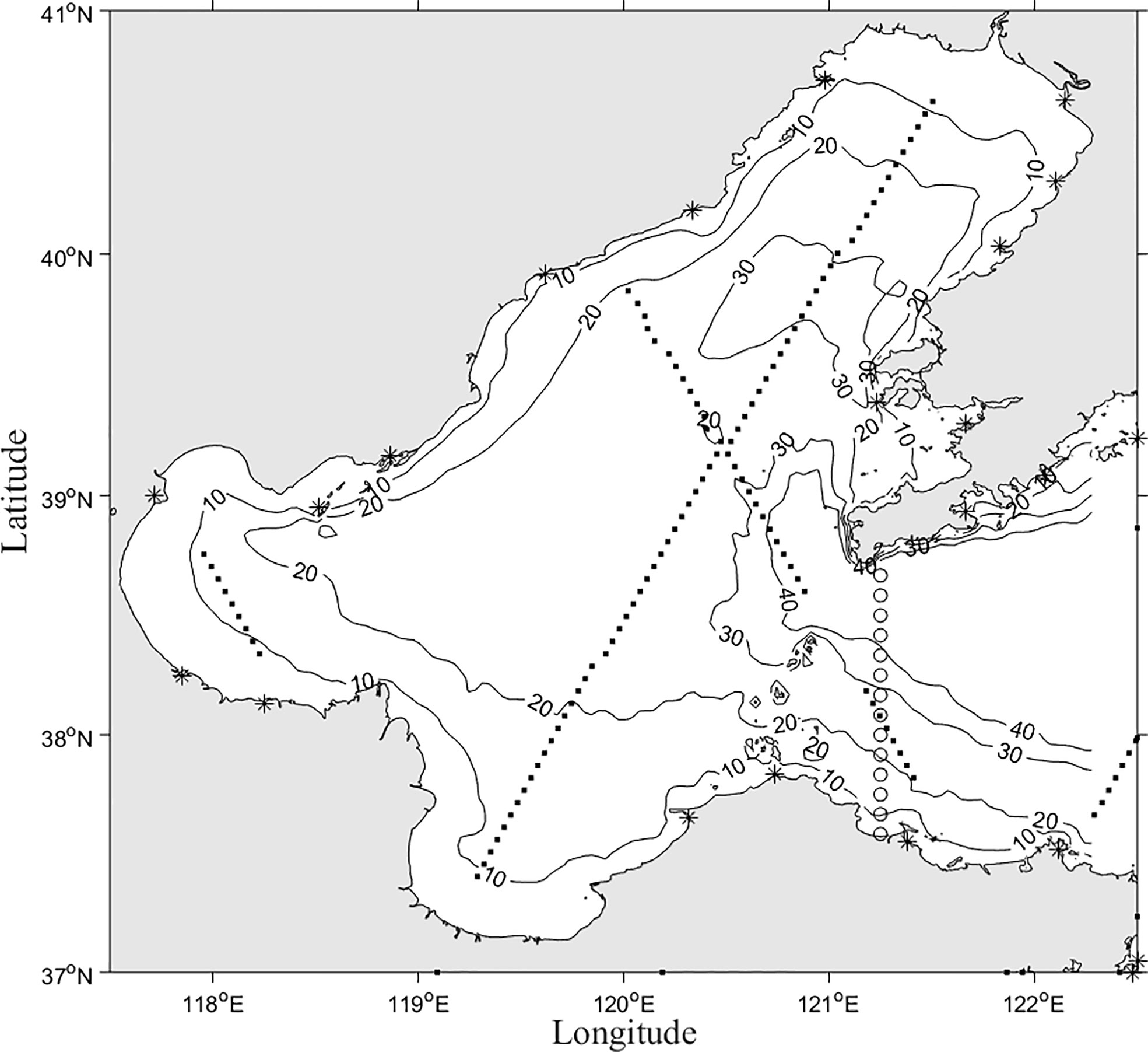
Figure 1 Bathymetry map of Bohai Sea and the position of tidal stations (asterisks), T/P-Jason altimeter tracks are denoted (points) and open boundaries (circles).

3 Method and process

Based on the 2-D tidal adjoint assimilation model, tidal constituents are simulated by assimilating different “simulated observations” to evaluate the different siting strategies of tidal stations. The process is described as follows.

1. Too dense distribution of tide stations will lead to low data acquisition efficiency. To ensure that the new tidal stations and the old ones are distributed as evenly as possible on the coastline of the Bohai Sea, the computational domain is divided into three subdomains, and experiments on different siting strategies are conducted in different subdomains. The specific subdomains and the corresponding gridded information are shown in Figure 2.

2. The OBCs and the spatial distribution of BFCs of M₂ constituent in the Bohai Sea are estimated (shown in Figures 3, 4) by assimilating tide gauges data and T/P-Jason altimeter data.

3. The HCs of the M₂ constituent at all computing grids (Figure 5) are calculated by using the OBCs and BFCs estimated in step (2). The grid points on the coastline are combined to determine different siting strategies. The HCs on the grid points in the siting strategies are served as SOs, which are used as the assimilation data in the subsequent experiments.

4. The HCs of the whole model domain are re-estimated by assimilating different combinations of SOs in different siting strategies. The re-estimation of HCs is achieved by inverting the OBCs and BFCs of M₂ constituent, of which the details will be described in the numerical experiments.

5. The root-mean-square (RMS) difference between SOs and re-estimated HCs is used to evaluate the effect of different strategies (Stammer et al., 2014; Zheng et al., 2020):

$\begin{array}{ll}\Delta r=\sqrt{\frac{1}{2N}{\displaystyle {\sum }_{i=1}^N\{{[H_{i}cos{\theta }_i-{\overline{H}}_{i}cos{\overline{\theta }}_i]}^2+{[H_i\sin {\theta }_i-{\overline{H}}_i\sin {\overline{\theta }}_i]}^2\}}}& (7)\end{array}$

where Δr is RMS difference, N represents the total number of SOs in each siting strategy, H_i and θ_i are the re-estimated HCs for the i-th point, and ${\overline{H}}_i$ and ${\overline{\theta }}_i$ are HCs of SOs. The RMS difference reflects the field-average deviation of model results, and a smaller RMS difference represents a possibly superior strategy. When the RMS difference is the smallest among all the siting strategies, the corresponding strategy is regarded as the optimum one.

FIGURE 2

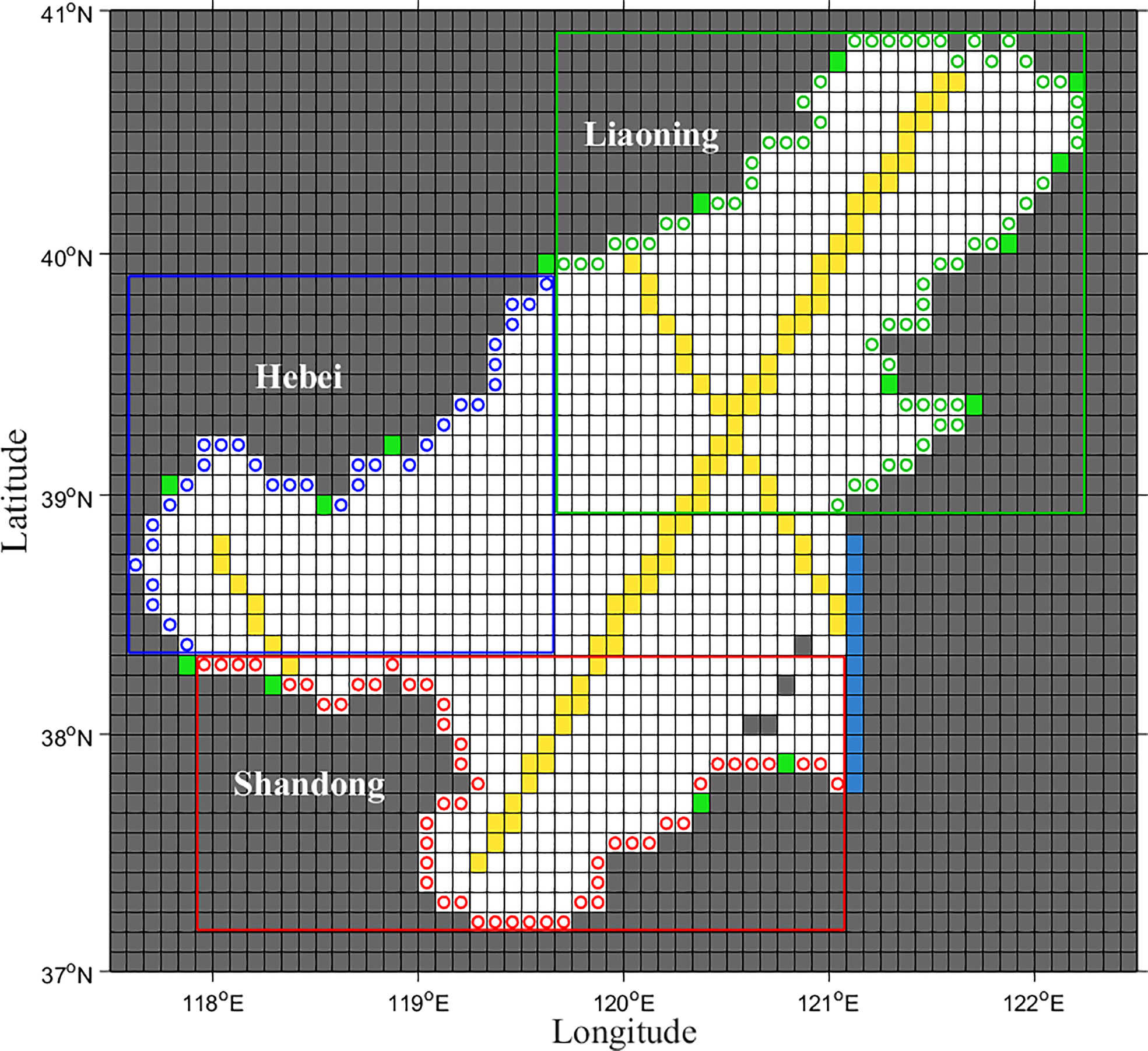
Figure 2 Grid map of different subdomains (circles with different colors represent coastline grids of different subdomains, the green grids represent existing tidal stations, the yellow grids represent TP-Jason altimeter tracks, the gray grids represent dry grid, and the white represents wet grids).

FIGURE 3

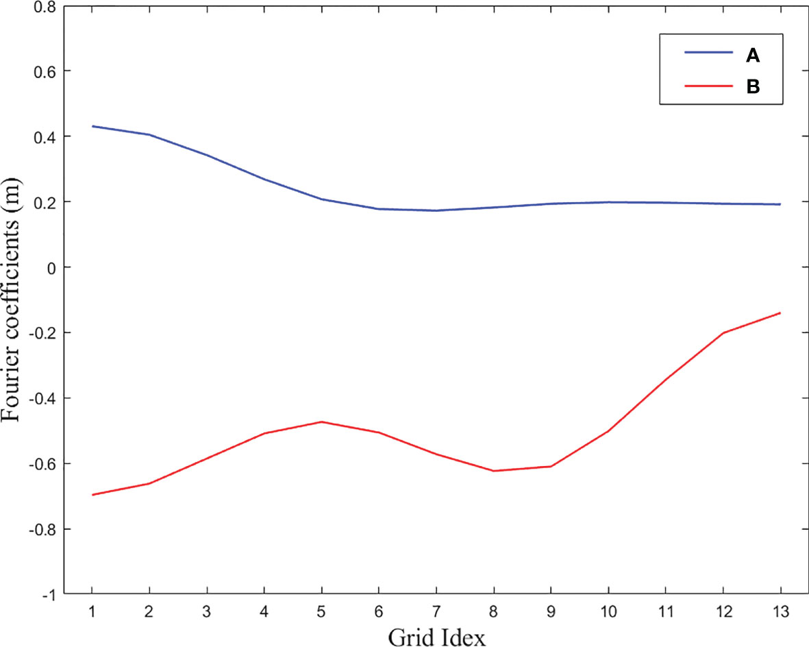
Figure 3 Estimated Fourier coefficients of OBCs for M₂ constituent in the Bohai Sea.

FIGURE 4

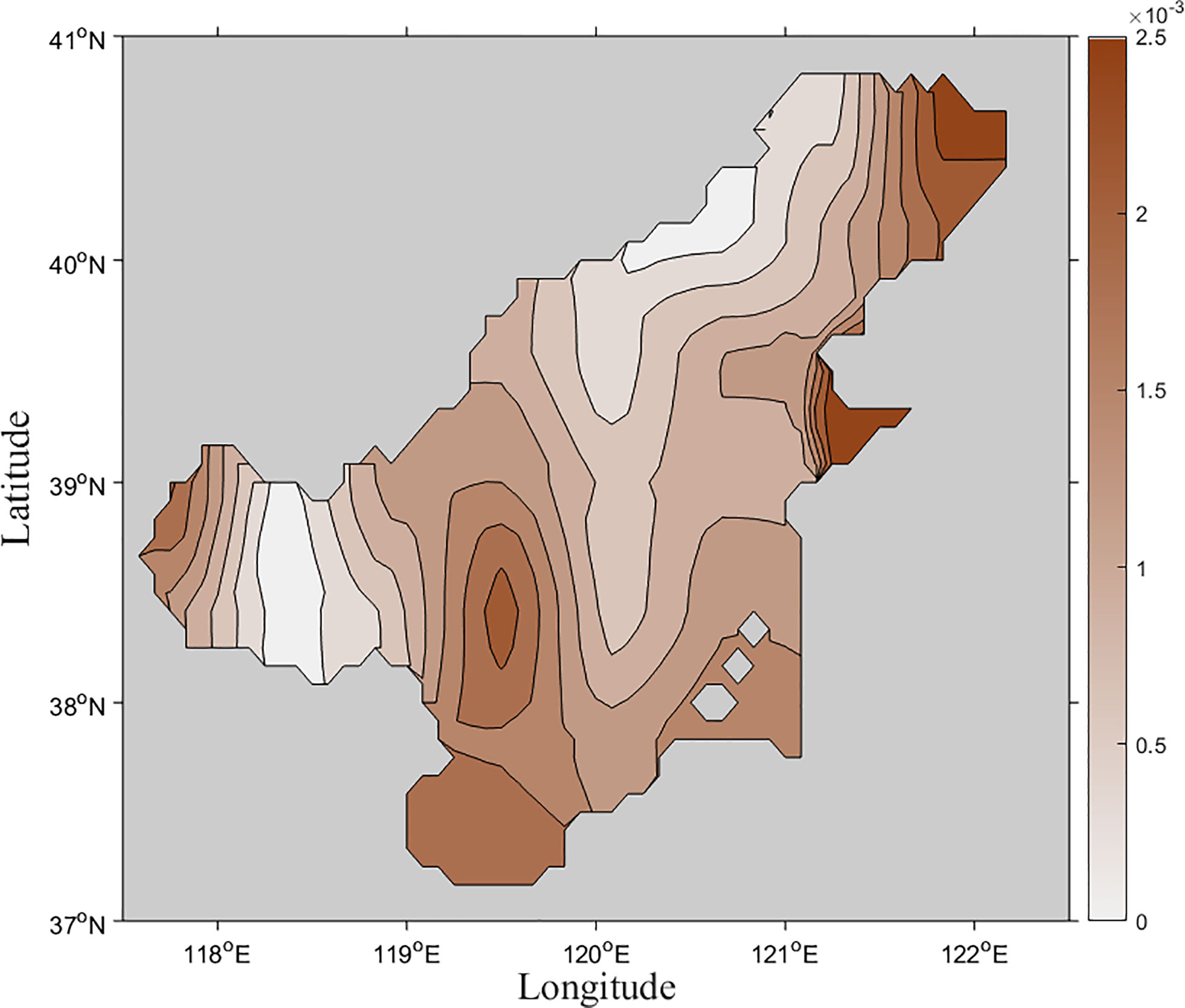
Figure 4 Estimated spatial distribution of BFCs for M₂ constituent in the Bohai Sea.

FIGURE 5

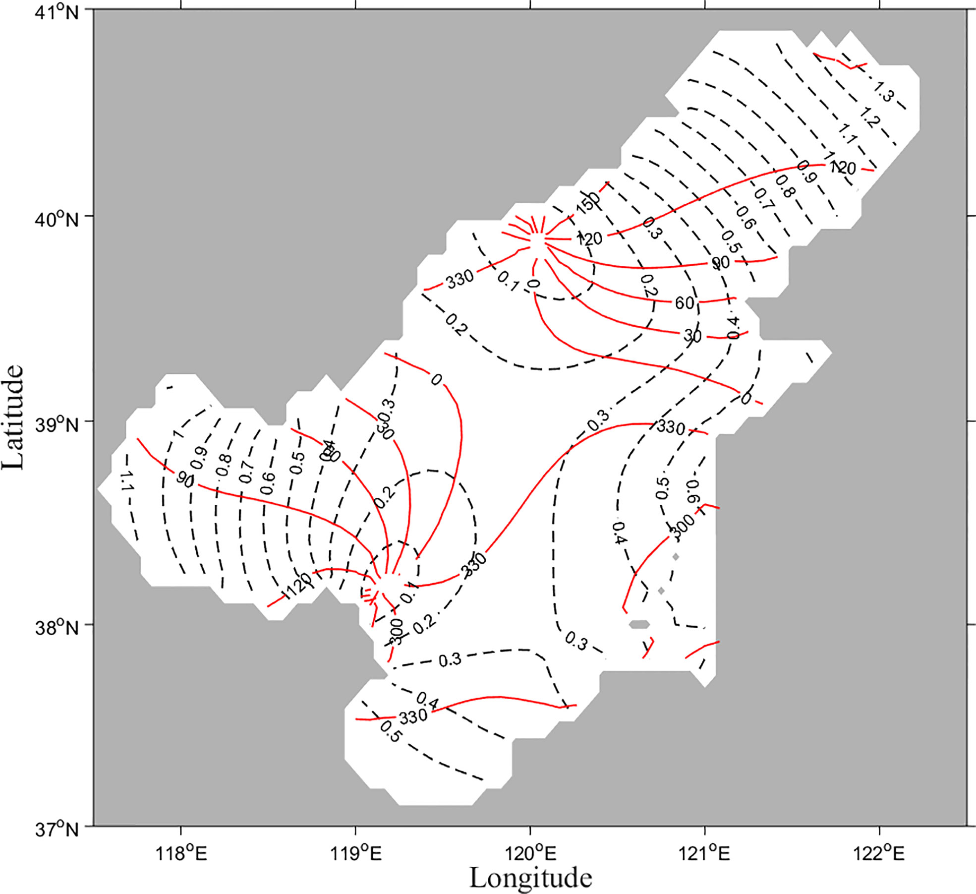
Figure 5 Co-tidal charts obtained with tidal station data and T/P-Jason altimeter data (dashed line denotes co-amplitude line (m), and solid line denotes the co-phase line (°)).

4 Numerical experiments

In this section, experiments are constructed to investigate the selection of siting scheme, the influence of different optimized variables in numerical simulation and the effect of siting strategies on the K₁ constituent, to determine the optimal siting selection strategy for new tidal stations in the Bohai Sea.

4.1 Uniform and non-uniform siting scheme selection

In this part, the subdomain in the south of the Bohai Sea (Figure 6) is selected as the research area. Four experiments are constructed, and the influences of the uniform and non-uniform siting schemes in data assimilation are investigated. Six new tidal stations are considered to be equidistantly distributed. In strategies 1-3, these stations are located in the west, south and east of Laizhou Bay, respectively. In strategy 4, these stations are uniformly located along the whole coastline of Laizhou Bay. Therefore, strategies 1-3 are regarded as non-uniform siting schemes and strategy 4 is the uniform one.The distributions of tidal stations in these strategies are displayed in Figure 6. To be more intuitive, the curved coastline is abstracted as a straight line.

FIGURE 6

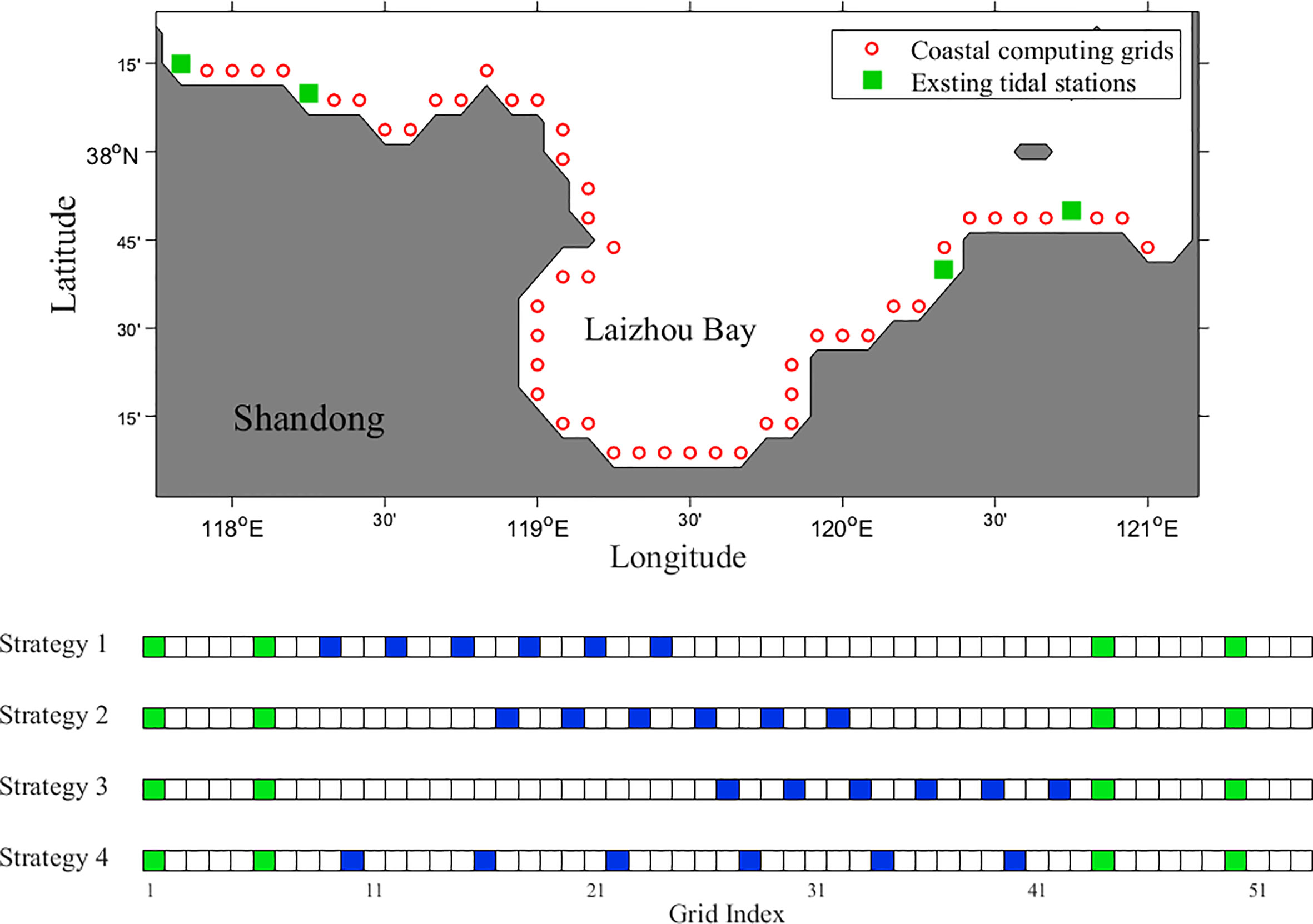
Figure 6 The map of subdomain in the south of the Bohai Sea and four different siting strategies in the form of grid (the green grids represent existing tidal stations and the blue grids represent new tidal stations).

For experiments of this subdomain, the BFCs remain unchanged, and the OBCs are inverted by assimilating SOs. The number of iteration steps is set to100, and the same step factor is used for different strategies. As shown in Table 1, the RMS differences between SOs and re-estimated HCs for the four strategies are calculated, and the mean absolute error (MAE) and root mean square error (RMSE) of HCs are also included as references.

$\begin{array}{ll}\text{MAE=}\frac{1}{N}{\displaystyle {\sum }_{i=1}^N|x_i-{\overline{x}}_i|}& (8)\end{array}$

$\begin{array}{ll}\text{RMSE=}\sqrt{\frac{1}{N}{\displaystyle {\sum }_{i=1}^N{(x_i-{\overline{x}}_i)}^2}}& (9)\end{array}$

TABLE 1

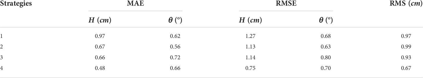
Table 1 Differences between SOs and re-estimated HCs for the four strategies.

where x_i represent the re-estimated HCs (H_i or θ_i ) for the i-th point, and ${\overline{x}}_i$ represent HCs of SOs (${\overline{H}}_i$ or ${\overline{\theta }}_i$ ).

The RMS difference of the M₂ constituent obtained with strategy 4 is 0.67 cm, which is the smallest among all these strategies. Similar results are also found for the MAE and RMSE. This result indicates that compared with the non-uniform siting, the uniform siting yields more accurate tidal characteristics in the Bohai Sea. Therefore, the new tidal stations are distributed uniformly along the coastline in the subsequent experiments.

4.2 Comparison of inversion variables

The subdomain in the west of the Bohai Sea (Figure 7) is selected as the research area to investigate the influence of inversion variables on siting strategies selection. There are 38 computing grids, 5 existing tidal stations, and 4 tidal stations to be sited. Four strategies are designed, and the distributions of tidal stations in these strategies are displayed in Figure 7.

FIGURE 7

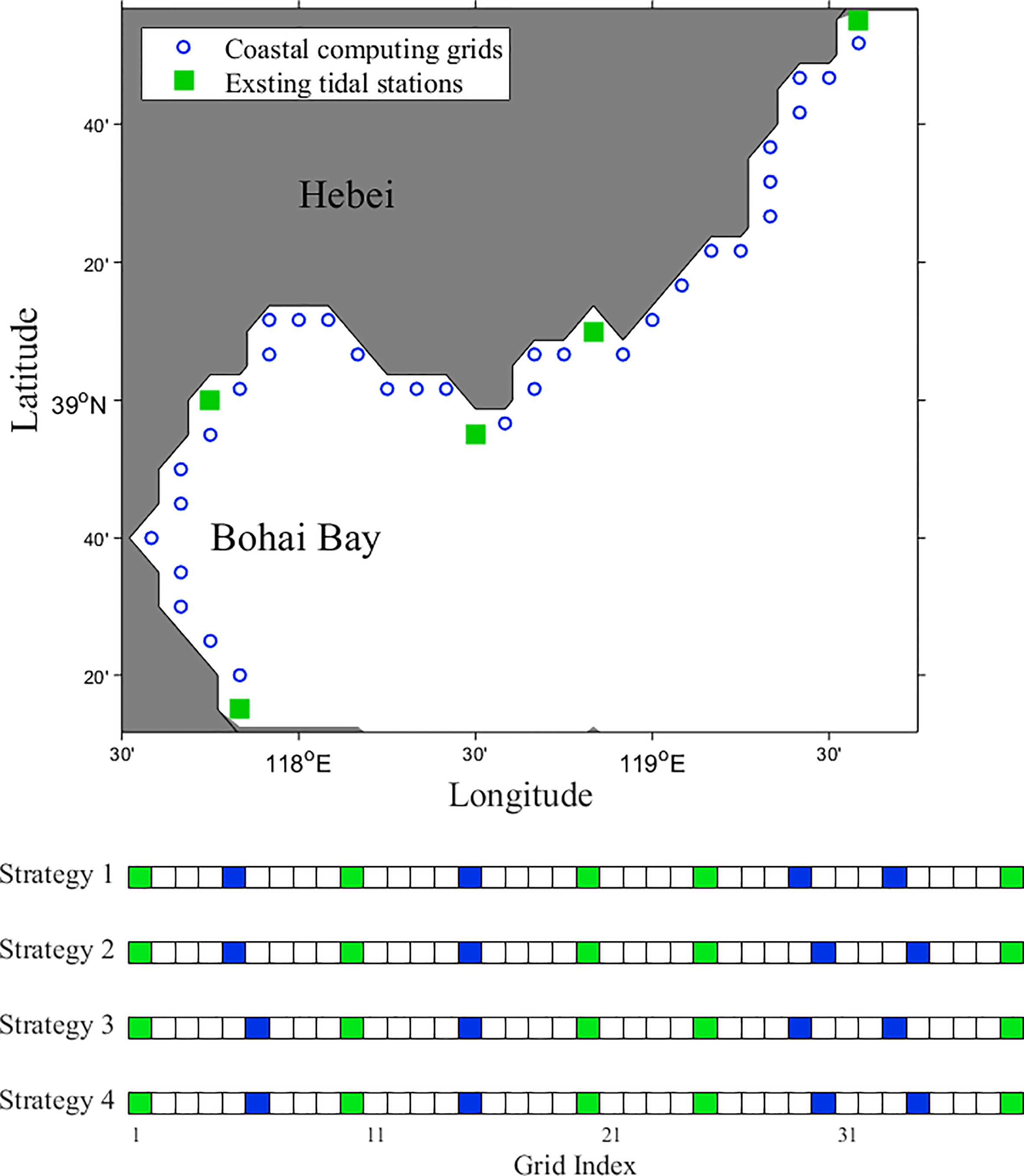
Figure 7 The map of subdomain in the west of the Bohai Sea and four different siting strategies in the form of grid (the green grids represent existing tidal stations and the blue grids represent new tidal stations).

In order to study the effect of different inversion variables on different siting strategies, two experimental schemes are constructed. First, the BFCs remain unchanged, and the OBCs are inverted by assimilating SOs. Second, the OBCs are kept unchanged and the BFCs are inverted by assimilating SOs. The number of iteration steps is set to100, and the same step factor is used for experiments in the same scheme. The difference between SOs and re-estimated HCs for each scheme are calculated, which are shown in Tables 2, 3.

TABLE 2

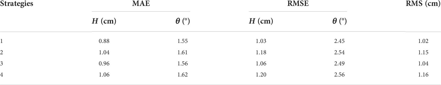
Table 2 Differences between SOs and re-estimated HCs obtained by inversion of OBCs.

TABLE 3

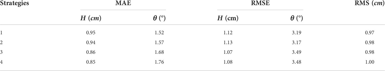
Table 3 Differences between SOs and re-estimated HCs obtained by inversion of BFCs.

The MEAs and RMSEs of H and θ are relatively small in experiments of inverting OBCs (Table 2), indicating that strategies 1 and 3 have a better effect. In experiments of inverting BFCs, strategies 1 and 2 have a better performance on θ, and strategies 3 and 4 have a better performance on H. However, for all these experiments, the RMS differences of strategy 1 are the smallest compared with the other strategies, which are 1.02 cm and 0.97 cm respectively. This result suggests that strategy 1 is a more suitable siting strategy for this subdomain. It is also worthy noted that the differences in all these strategies are generally on the same level, suggesting that the inversion variables do not have a great impact on the siting strategies.

4.3 Effect of siting strategies on different constituents

In tidal simulation and prediction, the HCs of main constituents must be determined, so main tidal constituents need to be included in this work. According to Fang et al. (2004), the M₂ constituent is the most significant semidiurnal tidal constituent in offshore China, and the K₁ constituent is the most significant diurnal tidal constituent. In this part, numerical simulations are carried out to study the effect of the siting strategies of new tidal stations for different tidal constituents. The subdomain in the north of the Bohai Sea (Figure 8) is selected as the research area, and 7 or 8 new tidal stations are sited on the coastline in the subdomain. A total of eight strategies are designed, and the distributions of tidal stations in these strategies are displayed in Figure 8.

FIGURE 8

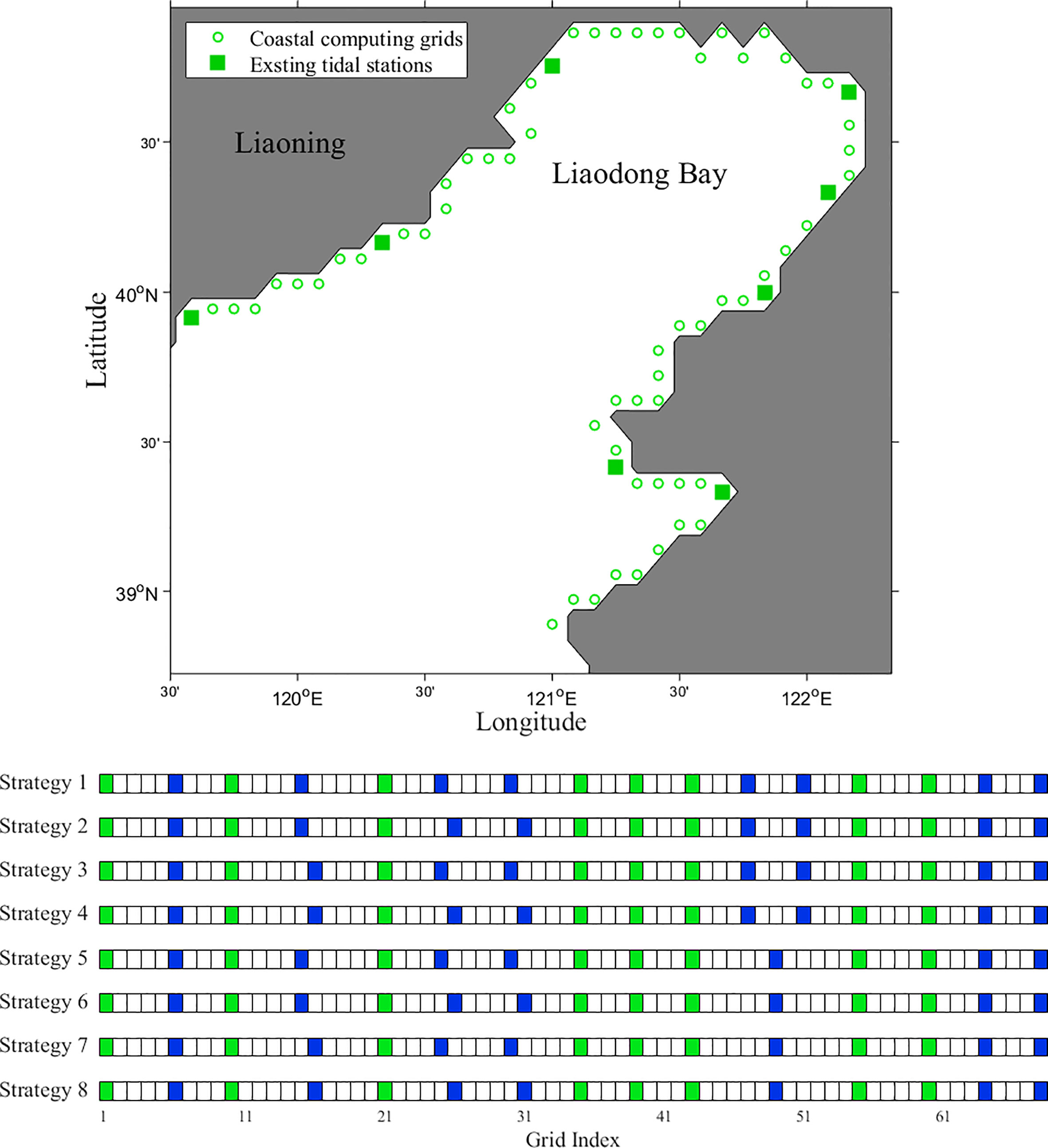
Figure 8 The map of subdomain in the north of the Bohai Sea and eight different siting strategies in the form of grid (the green grids represent existing tidal stations and the blue grids represent new tidal stations).

Experiments on the effect of different siting strategies on the M₂ tidal constituent are conducted by inverting OBCs, and the number of iteration steps is set to 100. For experiments of the K₁ constituent, the process is the same as described in Section 3, except that the observations are replaced by HCs of the K₁ constituent derived from T/P-Jason, and the number of iteration steps is set to 150. The differences between SOs and re-estimated HCs are shown in Tables 4, 5.

TABLE 4

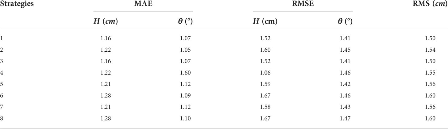
Table 4 Differences between SOs and re-estimated HCs of M₂ constituent.

TABLE 5

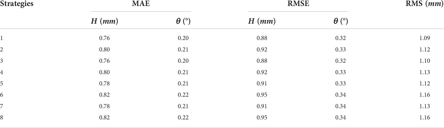
Table 5 Differences between SOs and re-estimated HCs of K₁ constituent.

The MEAs and RMSEs of the K₁ constituent are much smaller than those of the M₂ constituent. The RMS differences of the two constituents differ by an order of magnitude, which may be caused by their amplitude differences in the Bohai Sea. The averaged amplitude of the K₁ constituent is about 0.25 m, and the maximum amplitude is about 0.42 m. However, the average amplitude of the M₂ constituent is about 0.46 m, and the maximum amplitude is about 1.36 m.

According to Tables 4, 5, the effect of strategies 1~4 is better than that of strategies 5~8, which indicates that a reasonable increase in the number of tidal stations is beneficial for tidal numerical simulation and data assimilation. The RMS differences show that strategy 1 has the best performance. It is also worth noted that the RMS difference of strategy 3 is very close to that of strategy 1, suggesting that strategy 3 is a good alternative of strategy 1 for siting selection.

4.4 Conclusion of numerical experiments

The smaller the difference between observation and simulation, the better the effect of the data on model data assimilation, and the better the site selection strategy. Based on the experiments in this section, the optimum siting strategy for new tidal stations on the coastline in the southern, western and northern subdomains can be formulated, respectively. Combination of optimum strategies for the three subdomains serves as the optimum one for the Bohai Sea (Figure 9). According to the grid used in the computation, the reference latitude and longitude of 18 new tidal stations are given (Table 6). Taking the whole Bohai Sea as the experimental area, the HCs of the M₂ constituent are estimated by assimilating the SOs before and after the addition of the tidal stations separately. The RMS difference between the SOs and the re-estimated HCs decreased from 1.29 cm to 1.05 cm after the addition of the tidal station, with a decrease of 26.4%.

FIGURE 9

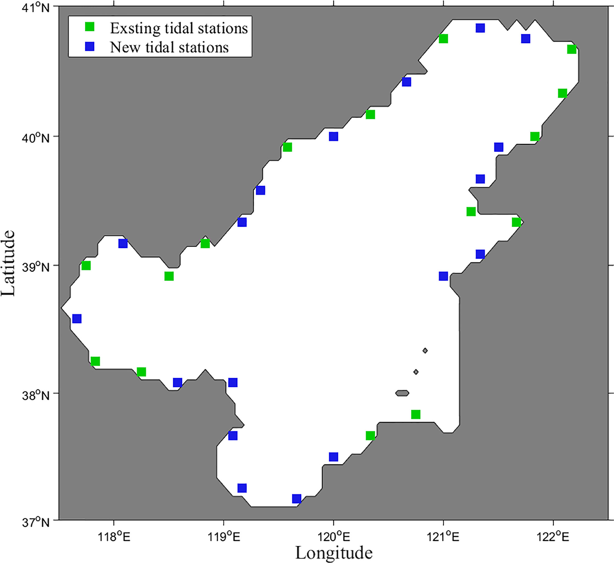
Figure 9 Grid map of new tidal station in the Bohai Sea (blue grids represent new tidal stations and the green grids represent existing tidal stations).

TABLE 6

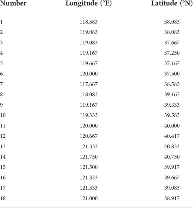
Table 6 Reference locations of new tidal stations based on computational grid.

This work is a reference for the siting of tidal stations in the Bohai Sea with a resolution of 5"×5" , which can be adapted to different needs by changing the resolution, the number of tidal stations, etc. The site selection process also needs to be integrated with the marine survey to adjust the reference locations.

5 Summary and discussion

The optimal siting of new tidal stations in the Bohai Sea is studied by using a 2-D tidal adjoint assimilation model. By assimilating the data of existing tide gauges and T/P-Jason altimeter, the OBCs and BFCs are optimized to obtain HCs of the M₂ constituent in the Bohai Sea, and the HCs at the newly added tidal stations on the coastline are used as the SOs for the subsequent experiments. The model domain is divided into three subdomains, and a series of experiments are conducted to determine the optimal siting strategy.

In the numerical experiments, the HCs are re-estimated by assimilating SOs, and the differences between re-estimated HCs and SOs are used to evaluate the effects of different strategies. Experiments in the southern subdomain reveal that a better effect is achieved by uniformly distributed tidal stations compared to a dense distribution when the number is the same. The effect of different inversion variables on the siting strategies is investigated in experiments of the western subdomain. Four siting strategies are designed, keeping the OBCs or BFCs constant and inverting the other to re-estimate the HCs for different strategies separately. The MAEs, RMSEs, and RMS differences of HCs are obtained by two experimental schemes of inverting OBCs and BFCs. The results of the four strategies are reflected differently in MAE and RMSE, but the reflection on the RMS differences is consistent, indicating that there is consistency in the experimental results across for the inverse variables. In the northern subdomain experiments, the effect of the siting strategies on the M₂ and K₁ constituents is studied. Experiments are also conducted on the K₁ constituent, and although the RMS differences of the K₁ constituent and the RMS differences of the M₂ constituent differ significantly, the experimental results show that the optimal strategy is the same. At the same time, results of these experiments confirm that adding observations at suitable locations facilitates tidal data assimilation and simulation.

According to the experimental results of three subdomains, the optimal strategy for the whole Bohai Sea is obtained by combining the optimal siting strategy on each coastline. The distribution map, latitude and longitude of tidal stations sties based on computational grid are also given. The results of the numerical experiments show that the effects of some strategies are very similar, which means that the reference location of the siting can be adjusted appropriately according to the geographical location, hydrological conditions and other elements. Combined with the investigation of hydrology and geology, this method provides great help for the site selection of tidal stations in the offshore area and the improvement of tide gauge data. It is believed that with further experiments and researches, the method can also be applied to a larger area of the ocean.

Data availability statement

Publicly available datasets were analyzed in this study. This data can be found here: https://www.aviso.altimetry.fr/en/data/products/auxiliary-products/coastal-tide-xtrack.html.

Author contributions

Conceptualization, XL. Methodology, XL. Software, SJ. Validation, SJ and HW. Formal analysis, HW and SJ. Investigation, HW. Writing—original draft preparation, HW and SJ. Writing—review and editing, XL. Supervision, XL. Project administration, XL. All authors contributed to the article and approved the submitted version.

Funding

This work is supported by the Natural Science Foundation of Shandong Province of China No. ZR2020MD056, the National Natural Science Foundation of China through grant 42076011 and U1806214, the National Key Research and Development Project of China through grant 2019YFC1408405.

Acknowledgments

The authors sincerely thank Qilin Zhang for his help in writing. We sincerely thank Song Gao, Jiangling Xu, Lingjuan Wu, and Dongling Guo for their support in data and methodology. We deeply thank the reviewers and editor for their constructive suggestions on the earlier version of the manuscript.

Conflict of interest

The authors declare that the research was conducted in the absence of any commercial or financial relationships that could be construed as a potential conflict of interest.

Publisher’s note

All claims expressed in this article are solely those of the authors and do not necessarily represent those of their affiliated organizations, or those of the publisher, the editors and the reviewers. Any product that may be evaluated in this article, or claim that may be made by its manufacturer, is not guaranteed or endorsed by the publisher.

References

Abessolo Ondoa G., Almar R., Castelle B., Testut L., Léger F., Sohou Z., et al. (2019). Sea Level at the coast from video-sensed waves: Comparison to tidal gauges and satellite altimetry. J. Atmos. Ocean. Technol. 36, 1591–1603. doi: 10.1175/JTECH-D-18-0203.1

CrossRef Full Text | Google Scholar

Adebisi N., Balogun A. L., Min T. H., Tella A. (2021). Advances in estimating Sea level rise: A review of tide gauge, satellite altimetry and spatial data science approaches. Ocean Coast. Manage. 208, 105632. doi: 10.1016/j.ocecoaman.2021.105632

CrossRef Full Text | Google Scholar

Andersen O. B., Neilsen K., Knudsen P., Hughes C. W., Bingham R., Fenoglio-Marc L., et al. (2018). Improving the coastal mean dynamic topography by geodetic combination of tide gauge and satellite altimetry. Mar. Geod. 41, 517–545. doi: 10.1080/01490419.2018.1530320

CrossRef Full Text | Google Scholar

Birol F., Fuller N., Lyard F., Cancet M., Niño F., Delebecque C., et al. (2016). Coastal applications from nadir altimetry: Example of the X-TRACK regional products. Adv. Sp. Res. 59, 936–953. doi: 10.1016/j.asr.2016.11.005

CrossRef Full Text | Google Scholar

Cao A., Guo Z., Lv X. (2012). Inversion of tidal open boundary conditions of the M₂ constituent in the bohai and yellow seas. Chin. J. Oceanol. Limnol. 30, 868–875. doi: 10.1007/s00343-012-1185-9

CrossRef Full Text | Google Scholar

Cheng Y., Plag H. P., Hamlington B. D., Xu Q., He Y. (2015). Regional sea level variability in the bohai Sea, yellow Sea, and East China Sea. Cont. Shelf Res. 111, 95–107. doi: 10.1016/j.csr.2015.11.005

CrossRef Full Text | Google Scholar

Chepurin G. A., Carton J. A., Leuliette E. (2014). Sea Level in ocean reanalyses and tide gauges. J. Geophys. Res. Ocean. 119, 147–155. doi: 10.1002/2013JC009365

CrossRef Full Text | Google Scholar

Egbert G. D., Ray R. D., Bills B. G. (2004). Numerical modeling of the global semidiurnal tide in the present day and in the last glacial maximum. J. Geophys. Res. Ocean. 109, 1–15. doi: 10.1029/2003jc001973

CrossRef Full Text | Google Scholar

Fang G., Wang Y., Wei Z., Choi B. H., Wang X., Wang J. (2004). Empirical cotidal charts of the bohai, yellow, and East China seas from 10 years of TOPEX/Poseidon altimetry. J. Geophys. Res. Ocean. 109, 1–13. doi: 10.1029/2004JC002484

CrossRef Full Text | Google Scholar

Feng J., Li D., Li Y., Liu Q., Wang A. (2018). Storm surge variation along the coast of the bohai Sea. Sci. Rep. 8, 1–10. doi: 10.1038/s41598-018-29712-z

PubMed Abstract | CrossRef Full Text | Google Scholar

Gao S., Xu J., Wu L., Guo D. (2016). Optimum strategy for siting of new tidal stations in the bohai Sea. Proc. 2016 Int. Conf. Appl. Mathematics Simulation Model., 260–264. doi: 10.2991/amsm-16.2016.58

CrossRef Full Text | Google Scholar

Guo Z., Pan H., Fan W., Lv X. (2017). Application of surface spline interpolation in inversion of bottom friction coefficients. J. Atmos. Ocean. Technol. 34, 2021–2028. doi: 10.1175/JTECH-D-17-0012.1

CrossRef Full Text | Google Scholar

He Y., Lu X., Qiu Z., Zhao J. (2004). Shallow water tidal constituents in the bohai Sea and the yellow Sea from a numerical adjoint model with TOPEX/POSEIDON altimeter data. Cont. Shelf Res. 24, 1521–1529. doi: 10.1016/j.csr.2004.05.008

CrossRef Full Text | Google Scholar

Khairuddin M. A., Din A. H. M., Omar A. H. (2019). Sea Level impact due to el nino and la nina phenomena from multi-mission satellite altimetry data over Malaysian seas. Lect. Notes Civ. Eng. 9, 771–792. doi: 10.1007/978-981-10-8016-6_57

CrossRef Full Text | Google Scholar

Lardner R. W. (1993). Optimal control of open boundary conditions for a numerical tidal model. Comput. Methods Appl. Mech. Eng. 102, 367–387. doi: 10.1016/0045-7825(93)90055-3

CrossRef Full Text | Google Scholar

Lardner R. W., Al-Rabeh A. H., Gunay N. (1993). Optimal estimation of parameters for a two-dimensional hydrodynamical model of the Arabian gulf. J. Geophys. Res. 98, 229–242. doi: 10.1029/93JC01411

CrossRef Full Text | Google Scholar

Liu K. X., Wang H., Fu S. J., Gao Z. G., Dong J. X., Feng J. L., et al. (2017). Evaluation of sea level rise in bohai bay and associated responses. Adv. Clim. Change Res. 8, 48–56. doi: 10.1016/j.accre.2017.03.006

CrossRef Full Text | Google Scholar

Lu X., Zhang J. (2006). Numerical study on spatially varying bottom friction coefficient of a 2D tidal model with adjoint method. Cont. Shelf Res. 26, 1905–1923. doi: 10.1016/j.csr.2006.06.007

CrossRef Full Text | Google Scholar

Lv X., Fang G. (2002). Numerical experiments of the adjoint model for M₂ tide in the bohai Sea. Acta Oceanol. Sincia. 24, 17–24.

Google Scholar

Madsen K., Høyer J., Fu W., Donlon C. (2015). Blending of satellite and tide gauge sea level observations and its assimilation in a storm surge model of the north Sea and Baltic Sea. J. Geophys. Res. Ocean. 120, 6405–6418. doi: 10.1002/2015JC011070

CrossRef Full Text | Google Scholar

Marcos M., Wöppelmann G., Matthews A., Ponte M. R., Birol F., Ardhuin F., et al. (2019). Coastal Sea level and related fields from existing observing systems. Surv. Geophys. 40, 1293–1317. doi: 10.1007/s10712-019-09513-3

CrossRef Full Text | Google Scholar

Pan H., Guo Z., Lv X. (2017). Inversion of tidal open boundary conditions of the M₂ constituent in the bohai and yellow seas. J. Atmos. Ocean. Technol. 34, 1661–1672. doi: 10.1175/JTECH-D-16-0238.1

CrossRef Full Text | Google Scholar

Piecuch C. G., Huybers P., Tingley M. P. (2017). Comparison of full and empirical bayes approaches for inferring sea-level changes from tide-gauge data. J. Geophys. Res. Ocean. 122, 2243–2258. doi: 10.1002/2016JC012506

CrossRef Full Text | Google Scholar

Qu Y., Jevrejeva S., Jackson L. P., Moore J. C. (2019). Coastal Sea level rise around the China seas. Glob. Planet. Change 172, 454–463. doi: 10.1016/j.gloplacha.2018.11.005

CrossRef Full Text | Google Scholar

Sannino G., Bargagli A., Artale V. (2004). Numerical modeling of the semidiurnal tidal exchange through the strait of Gibraltar. J. Geophys. Res. Ocean. 109, 1–23. doi: 10.1029/2003JC002057

CrossRef Full Text | Google Scholar

Seiler U. (1993). Estimation of open boundary conditions with the adjoint method. J. Geophys. Res. 98, :22855-22870. doi: 10.1029/93jc02376

CrossRef Full Text | Google Scholar

Spada G., Galassi G., Olivieri M. (2014). A study of the longest tide gauge sea-level record in Greenland (Nuuk/Godthab 1958-2002). Glob. Planet. Change 118, 42–51. doi: 10.1016/j.gloplacha.2014.04.001

CrossRef Full Text | Google Scholar

Stammer D., Ray R. D., Andersen O. B., Arbic B. K., Bosch W., Carrère L., et al. (2014). Accuracy assessment of global barotropic ocean tide models. Rev. Geophys. 52, 243–282. doi: 10.1002/2014RG000450

CrossRef Full Text | Google Scholar

Trupin A., Wahr J. (1990). Spectroscopic analysis of global tide gauge sea level data. Geophys. J. Int. 100, 441–453. doi: 10.1111/j.1365-246X.1990.tb00697.x

CrossRef Full Text | Google Scholar

Wang D., Liu Q., Lv X. (2014). A study on bottom friction coefficient in the bohai, yellow, and East China Sea. Math. Probl. Eng. 2014, 2–9. doi: 10.1155/2014/432529

CrossRef Full Text | Google Scholar

Wang D., Zhang J., Mu L. (2021). A feature point scheme for improving estimation of the temporally varying bottom friction coefficient in tidal models using adjoint method. Ocean Eng. 220, 108481. doi: 10.1016/j.oceaneng.2020.108481

CrossRef Full Text | Google Scholar

Xu P., Mao X., Jiang W. (2017). Estimation of the bottom stress and bottom drag coefficient in a highly asymmetric tidal bay using three independent methods. Cont. Shelf Res. 140, 37–46. doi: 10.1016/j.csr.2017.04.004

CrossRef Full Text | Google Scholar

Yum S. G., Wei H. H., Jang S. H. (2021). Estimation of the non-exceedance probability of extreme storm surges in south Korea using tidal-gauge data. Nat. Hazards Earth Syst. Sci. 21, 2611–2631. doi: 10.5194/nhess-21-2611-2021

CrossRef Full Text | Google Scholar

Zhang J., Lu X. (2010). Inversion of three-dimensional tidal currents in marginal seas by assimilating satellite altimetry. Comput. Methods Appl. Mech. Eng. 199, 3125–3136. doi: 10.1016/j.cma.2010.06.014

CrossRef Full Text | Google Scholar

Zhao P., Jiang W. (2011). A numerical study of storm surges caused by cold-air outbreaks in the bohai Sea. Nat. Hazards 59, 1–15. doi: 10.1007/s11069-010-9690-7

CrossRef Full Text | Google Scholar

Zheng J., Mao X., Lv X., Jiang W. (2020). The M₂ cotidal chart in the bohai, yellow, and east china seas from dynamically constrained interpolation. J. Atmos. Ocean. Technol. 37, 1219–1229. doi: 10.1175/JTECH-D-19-0212.1

CrossRef Full Text | Google Scholar