Spatial-digital joint self-interference cancellation method for in-band full-duplex underwater acoustic communication

The in-band full-duplex underwater acoustic communication (IBFD-UWAC) mode has twice the information throughput of the traditional half-duplex communication mode, significantly increasing the communication efficiency. Extracting the weak desired signal from the high-power self-interference signal without distortion remains a challenging problem in implementing IBFD-UWAC systems. This paper proposes a spatial-digital joint self-interference cancellation (SDSIC) method for IBFD-UWAC. We first perform spatial self-interference cancellation (SSIC) and propose an improved wideband constant-beamwidth beamformer to overcome the problem of direction- and array-dependent interference in IBFD-UWAC systems. Convex optimization is used to maintain a constant beam response in the main flap and cancel the self-interference signal from a fixed direction, thus increasing the signal-to-interference ratio of the desired signal. Subsequently, we perform digital self-interference cancellation (DSIC) on the residual self-interference signal, and propose a variable-step-size least-mean-squares algorithm based on the spatial noise threshold. This algorithm modifies the least-mean-squares step-size adjustment criterion according to the noise level after SSIC and the desired signal, resulting in better DSIC. A series of simulations are implemented in a hardware-in-the-loop platform to verify the practicality and real-time performance of the proposed SDSIC method. The results show that the self-interference signal power can be reduced by 41.5 dB using the proposed method, an improvement of 13.5 dB over the conventional SIC method.

1 Introduction

Recently, considerable attention has focused on underwater communication. Although there are numerous communication network protocols, mature land-based wireless network protocols often fail in underwater communication networks due to the long transmission delays, limited bandwidth, and the large spatial and temporal variability of the underwater acoustic channel (Yin, 2016; Song et al., 2019; Zhao et al., 2021). The scarce spectrum resources of the underwater acoustic channel also limit the frequency efficiency of underwater communication networks (Pan et al., 2012; Yan et al., 2021). Therefore, improving the spectrum efficiency and system information throughput of underwater acoustic communication (UWAC) networks under severe bandwidth limitations is an urgent problem. In-band full-duplex (IBFD) UWAC technology aims to achieve simultaneous transmission and reception of signals in the same frequency band from both sides of the communication. Compared with the traditional half-duplex mode, this increases the frequency efficiency by a factor of two, and increases the security of the communication system (Qiao et al., 2018a; Kolodziej et al., 2019). In engineering applications, IBFD-UWAC systems are typically used as relay nodes that receive data from one party while forwarding it to another party when the far-end desired signal is buried in high-power self-interference (SI) and communication cannot be achieved. To realize IBFD-UWAC, it is necessary to cancel the local high-power near-end SI signals (Sabharwal et al., 2014; Shen et al., 2020) and increase the signal-to-interference noise ratio (SINR) of the weak desired far-end signals to enable real-time communication between the two sides (Zhang et al., 2016; Zhao, 2021). Therefore, self-interference cancellation (SIC) is a critical technical issue. Spatial SIC (SSIC) is the first stage of the SIC process in IBFD-UWAC systems. The SSIC process does not attempt to perfectly cancel SI, but instead seeks to reduce SI by a sufficient amount to prevent the receiver’s dynamic range from being swamped. After the SSIC process, a residual interference signal (RIS) remains. Digital SIC (DSIC) is needed to cancel the RIS (Everett et al., 2016; Satyanarayana et al., 2019).

For the SSIC method in full-duplex communication, a two-transmitter, three-receiver antenna system has been designed to provide 50 dB additional isolation, compared with a single-transmitter, single-receiver system, by adjusting the amplitude and phase of the transmitting and receiving antennas (Snow et al., 2011). Additionally, a compact switched-array reconfigurable antenna array has achieved a 65 dB passive SIC based on 10-cm transmitter and receiver antenna isolation (Ahmed and Eltawil, 2015). Vallese et al. (2017) proposed a joint transceiver–receiver beamforming algorithm for co-time, co-frequency full-duplex wireless communication systems, with SIC effects of 65.5 dB and 89.8 dB at transmitter signal-to-noise ratios (SNRs) of 30.0 dB and 60.0 dB, respectively. Everett et al. (2014) terminated the passive SIC effects in the radio carrier frequency range of 2.4–2.48 GHz at different distances. They obtained 27.9 dB and 24.5 dB interference cancellation effects at 50 cm and 35 cm, respectively, using an omnidirectional transmitting antenna. An additional 17 dB interference cancellation effect with a 90°-beamwidth transmitting antenna and 50 cm between the receiving and transmitting antennas was achieved by combining the directional antenna, absorbing medium, and antenna polarization. This resulted in interference cancellation of more than 70 dB and showed that passive cancellation performance is affected by the number of reflected paths (Everett et al., 2014). Choi et al. (2010) placed two transmit antennas half a wavelength away from a single receive antenna to achieve mutual cancellation. They conducted experiments at 2.4 GHz using a 7-inch antenna, and found that this configuration provided 26 dB of interference cancellation (5 MHz). The combination of noise cancellation and DSIC produced an overall SIC of 60 dB, but the results were not satisfactory for signal bandwidths over 100 MHz (Choi et al., 2010). Nawaz and Tekin (2016) designed and implemented a 2.4-GHz bipolar micro-bandwidth patch antenna, and evaluated its isolation performance. The results showed that the antenna could achieve 40 dB of interference cancellation. Cacciola et al. (2016) completely embedded the transmitting and receiving arrays in a metallic cavity and mounted them flush on the ground to reduce the interaction with nearby objects and antennas. This method obtained interference cancellation of more than 49 dB. Makar et al. (2017) proposed a toroidal hybrid T-shaped structure with a length of 35.6 mm that obtained an SIC effect of at least 35 dB in a multipath environment with near-omnidirectional transmitting and receiving antennas.

However, the above SSIC methods have been developed in the field of radio communication. In the engineering implementation of underwater communication, the equipment used for SSIC, such as acoustic baffles, has different apertures corresponding to different absorption frequencies, which attenuate the sound power by reflecting the sound within them. Qiao et al. (2013) used the vector hydrophone zero-point offset feature to reduce the received SI signal power. The full-duplex UWAC system developed by Li et al. (2015) uses a transmitting transducer with directivity (Zhao et al., 2021) to obtain an interference cancellation effect of about 25 dB. While acoustic baffles are inconvenient in engineering applications because of their weight and volume, directivity transducers are hardware-dependent. frequencies and attenuate the sound power by reflecting sound in them. They have limited cancellation capability and less flexibility, so the cancellation of local SI by array signal processing technology in wideband communication systems is worthy of study, but no SSIC scheme based on array signal processing has yet been proposed for IBFD-UWAC systems. This paper proposes an improved constant beamwidth beamforming (ICBBF) algorithm.

For DSIC, Qiao et al. (2018b) proposed a maximum-likelihood algorithm with sparse constraints for estimating the sparse SI channels, achieving an SIC effect of 43 dB. This is a better cancellation effect than the least-squares algorithm. In the same year, Qiao et al. (2018a) considered the high probability of non-crossover regions for the transceiver signals during normal IBFD-UWAC, and proposed a DSIC algorithm for asynchronous full-duplex communication systems. This algorithm used non-crossover regions to collect the nonlinear distortion components combined with a sparse adaptive channel estimation algorithm for SIC. Their experimental results show that the method can effectively eliminate the nonlinear distortion caused by the power amplifier (PA). Shen et al. (2020) used the PA output channel signal as a reference and applied the dichotomous coordinate descent recursive least-squares (DCD-RLS) algorithm (Zakharov et al., 2008), which has a convergence rate similar to that of classical RLS. The complexity can be effectively reduced with the same numerical stability. Experiments show that the DCD-RLS algorithm achieves 46 dB cancellation, while an additional 23 dB SIC performance is obtained when the PA output channel signal is used as the reference signal. Note that nonlinear devices other than amplifiers have a limiting effect on this method, such as preamplifiers (Liu et al., 2009).

The literature discussed above is focused on the convergence speed of the algorithm and the cancellation effect of the DSIC process, with little consideration of the impact of algorithm complexity in real time. The real-time implementation of IBFD-UWAC systems would allow both parties to communicate without delay and with no need to wait for the algorithm process, which is of great significance. In addition, the signal-to-interference ratio (SIR) of the signal is still low after the SI signal is canceled by SSIC or the analog domain, leaving the RIS. In IBFD-UWAC systems, the performance of interference cancellation depends on the accuracy of interference propagation channel estimation, the desired signal can have an impact on the self-interference channel estimation process, resulting in a lower bit error rate (BER) performance (Qiao et al., 2018a). During the SI channel estimation process, previous studies do not consider the impact of the arrival of the desired signal, causing a reduction in BER performance.

Based on the above, this paper makes the following contributions.

● For SIC in IBFD-UWAC systems, this paper proposes a spatial-digital joint SIC (SDSIC) method that achieves better cancellation than the previous SIC.

● We propose an SSIC method using an ICBBF based on convex optimization theory for IBFD-UWAC systems. This SIC method prevents the distortion of the distant desired signal and suppresses the direction- and array-dependent interference.

● For DSIC, a variable-step-size least-mean-square algorithm based on the space domain noise threshold (SNT-VSS-LMS) is proposed. This method has a faster convergence speed and better cancellation effect than the general VSS-LMS method.

2 System model

The modulated signal x[n] is transmitted by a digital-to-analog converter (DAC). After passing through a low-pass filter (LPF) and PA, the signal is transmitted by the transducer, and the transmitted signal r_n(t) is received by the array after passing through the SI channel h_SI[n] , while the remote desired signal r_m(t) is received by the array. Thus, the array received signal x_m(t) is obtained as

$\begin{array}{ll}{x}_{\text{m}}(t)=r_{n\text{m}}(t)+r_{f\text{m}}(t)+n_{\text{m}}(t)& (1)\end{array}$

Where, m=1,2,3,⋯,M , r_nm(t) is the local SI signal received by array element m, r_fm(t) is the desired signal received by array element m, and n_xtm(t) is the ambient noise received by array element m. The purpose of SIC is to reconstruct the SI signal so that r_n(t) can be subtracted from the received signal to obtain the pure desired signal. After being received by the array, the signals from different directional sources have different time delays. The purpose of SSIC is to use these time delays to increase the SINR. The received signal is acquired by an analog-to-digital converter (ADC) after a low-noise amplifier (LNA) and passed through the beamformer to obtain the RIS after the SSIC process (① in Figure 1). In the DSIC process (position ② in Figure 1), the RIS is compared with the reference beamformer. The RIS is passed through a linear filter together with the reference signal to complete the DSIC process. To consider the effect of the nonlinear distortion of the PA on the estimation process of the SI channel, ${y^{\prime }}_{\text{PA}}\left[n\right]$ is passed through an adaptive filter together with the RIS to obtain the estimated SI channel ${\widehat{h}}_{\text{SI}}$ and the reconstructed SI signal y_tASIC[n] , where y_ASIC[n] is related to ${\widehat{h}}_{\text{SI}}$ as follows. The error output of the filter e(n) is the signal after DSIC, which is the desired signal to be demodulated. The error output can be written as

$\begin{array}{ll}e(n)=r_{AB}(n)-{y^{\prime }}_{\text{PA}}\otimes {\widehat{h}}_{\text{SI}}& (2)\end{array}$

FIGURE 1

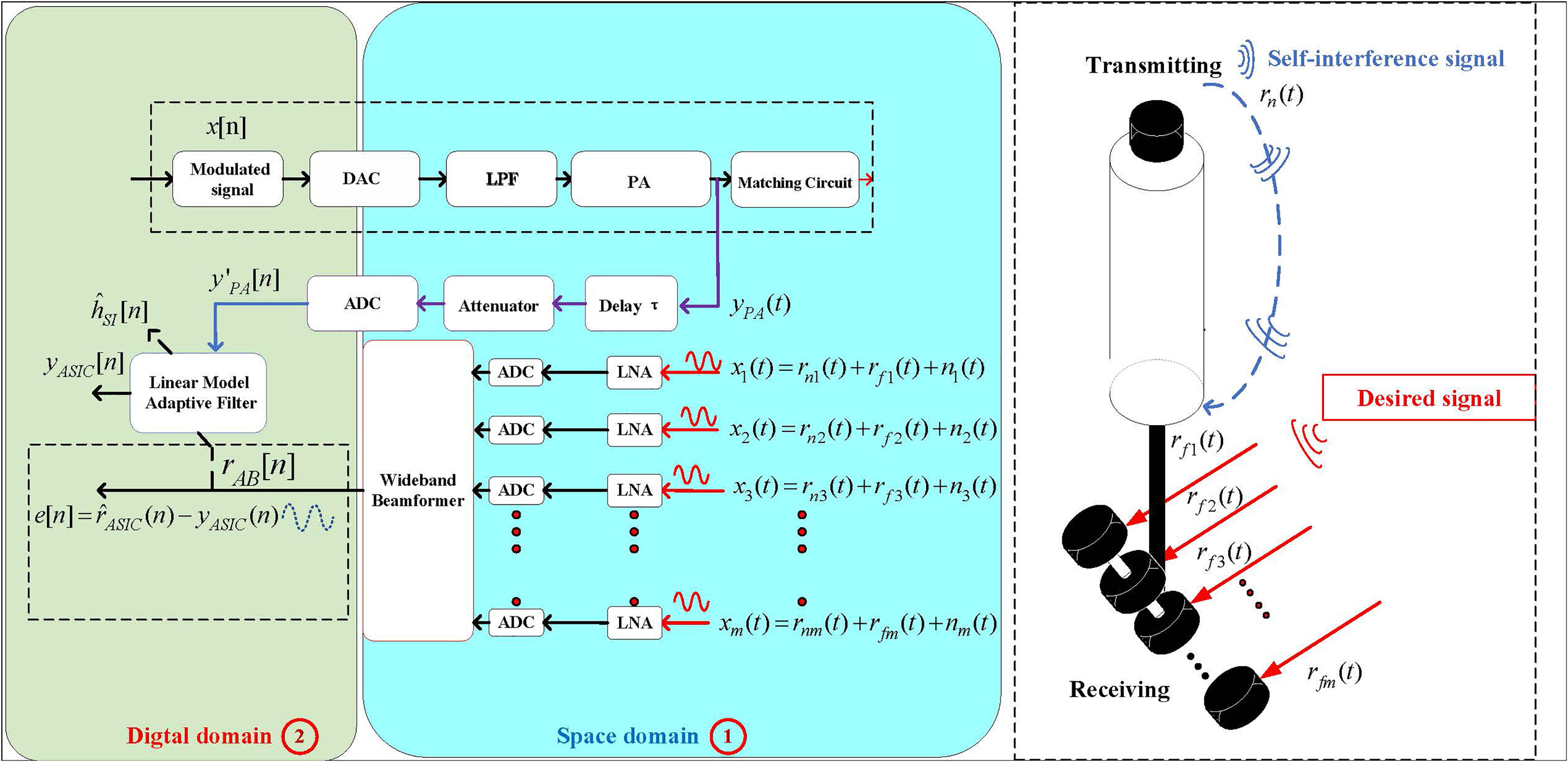
Figure 1 SDSIC system model in IBFD-UWAC.

where ⊗ denotes the convolution operation. The reference signal vector ${y^{\prime }}_{\text{PA}}$ and the tap weights of the linear filter are

$${y^{\prime }}_{\text{ PA}}=\left[{y^{\prime }}_{\text{ PA}}[n],{y^{\prime }}_{\text{ PA}}[n-1],\dots ,{y^{\prime }}_{\text{ PA}}[n-L+1]\right]$$

$\begin{array}{ll}{\widehat{h}}_{\text{SI}}=\left[{\tilde{h}}_{\text{SI}}[n],{\tilde{h}}_{\text{SI}}[n-1],\dots ,{\tilde{h}}_{\text{SI}}[n-L+1]\right]& (3)\end{array}$

where L is the number of tap weights of the linear filter. The DSIC performance in the IBFD-UWAC system depends on approximation with y_ASIC(t) and y_PA(t) . The above DSIC process is position 173 in the system model of Figure 1.

3 Fundamentals

3.1 Spatial self-interference cancellation

Beamforming is a common interference cancellation technique that is widely used in radio and underwater acoustics. This paper focuses on the IBFD-UWAC system. After receiving the signal, beamforming is performed in the spatial domain for SIC and to increase the SIR of the received signal. For UWAC systems, the acoustic waves are spatially sampled by M array elements, and the output signal y(t) from the system at time t is the instantaneous linear combination of the spatial samples x_m(t) , that is,

$\begin{array}{ll}y(t)=\sum _{m=1}^M{x}_m(t)w_m^{*}& (4)\end{array}$

where w_m denotes the weight coefficient of array element m and * denotes the complex conjugate. Let the input signal be the impulsive complex plane wave e^jωt , which has angular frequency ω, and let the arrival angle be θ∈[−π/2,π/2t]θθ∈[−π/2,π/2] . Assume that the signal phase received by the first array element is 0, and the signal received by the first array element is x₀(t)=e^jωt . The signal received by array element m is x_m(t)=e^jωt−τ_m , where the time delay in the wave from the first hydrophone to the m-th hydrophone is τ_m , which a function of the arrival angle θ. The beamformer output can be expressed by

$\begin{array}{ll}y(t)=e^{j\omega t}\sum _{m=1}^M{e}^{(-\omega {\tau }_m)}{w}_m^{*}& (5)\end{array}$

where τ₀=0 and $j=\sqrt{-1}$. The response of the beamformer is

$\begin{array}{ll}P\omega ,\theta =\sum _{\text{m}=1}^M{e}^{(-\omega {\tau }_m)}{w}_m^{*}=w^{H}a(\omega ,\theta )& (6)\end{array}$

where the vector w contains the complex conjugate coefficients of the M sensors and H denotes the conjugate transpose, i.e.,

$\begin{array}{ll}w={[w_1,w_2,w_3\cdots w_M]}^T& (7)\end{array}$

in which T denotes the transpose. The vector a(ω,θ) is the array response vector, also known as the guide vector, i.e.,

$\begin{array}{ll}a(\omega ,\theta )=[1,e^{-j\omega {\tau }_1},e^{-j\omega {\tau }_2}\cdots e^{-j\omega {\tau }_{M-1}}]& (8)\end{array}$

The distance between each array element is d=λ/2 , and so ωτ_m=(2πc/λ)(mdsin θ/c)=mπsin θ . The narrowband beamformer response is written as

$\begin{array}{ll}\text{P}(\omega ,\theta )=\sum _{\text{m}=1}^M{e}^{(-j\text{m}\pi \sin \theta )}{w}_m^{*}& (9)\end{array}$

Note that the SSIC method uses a frequency-domain wideband beamformer to convert the data from the time domain to multiple sub-bands in the frequency domain through a Fourier transform. Each sub-band satisfies the narrowband condition to finish the beamforming process. Finally, the output of the beamformer is transformed to the time domain using an inverse discrete Fourier transform. For the problem of an inconsistent response at each frequency point, one method involves receiving the data of each frequency of the signal with different sizes of sub-arrays (Goodwin and Elko, 1993; Liu et al., 2021), but this requires a complex hardware structure and cannot achieve a constant beamwidth for the whole frequency band. More recently, researchers have designed different weighting vectors for the various sub-band frequencies, resulting in a constant beamwidth at these central frequencies. There are spatial re-sampling methods (Krolik and Swingler, 1990; Li et al., 2017), fitting methods based on Fourier transforms (Liu et al., 2007; Chan and Chen, 2007; Liu and Weiss, 2008), and Bessel function algorithms (Liu et al., 2005), among others. Furthermore, in the practical application of IBFD-UWAC systems, it is often necessary to design a special response beamformer according to the array shape (Roe et al., 1990; Fan and Liang, 2013). This process mainly keeps the main flap beam response consistent and suppresses direction- and array-dependent interference. In practical applications, if there are multiple desired signals at unknown angles in the far field, the beamformer should be designed such that the beam response of the side flaps can discriminate the multiple desired signals in different directions, which is critical for a full-duplex communication network. To solve the above problems, an ICBBF based on convex optimization theory is proposed in this paper. The proposed beamforming method constructs a “zero trap” for direction- and array-dependent interference source directions while maintaining the frequency invariance of the beam response of the main flap. We design the convex optimization process as follows. It is worth noting that the beamformer avoids significant amplitude cancellation of signals from other angles and retains the signal from other directions. The SSIC method designed in this paper uses a convex optimization method to cancel the SI signals of direction- and array-dependent interference in the IBFD-UWAC system. We design the specific convex optimization process as follows. Step 1: Apply Newton’s iteration method to produce a beamformer according to the array structure, where the desired signal source angle is 0°, and divide the signal into several sub-bands. Perform the following steps at each sub-band frequency. Step 2: Take the main flap response at the center frequency of the beamformer designed above as the desired response p_desired(θ) for the convex optimization process, and minimize the two-parameter response of the optimized beamformer response p_MF(θ) in the main flap angle interval θ_MF with p_desired(θ) . Step 3: Use convex optimization theory to constrain the beam response p_SF(θ) in the side flap angle interval θ_SF to be below the set value ξ_SF and the beam response p_ZF(θ) in the zero-trap interval θ_ZF below the set value ξ_ZF . Step 4: Use an inverse fast Fourier transform to restore the signal and obtain the signal after SSIC. According to the above steps, we construct the convex optimization equation as

$\begin{array}{ll}\begin{array}{l}\underset{{\omega }_{HB}}{\min }{\Vert p_{MF}(\theta )-p_{desired}(\theta )\Vert }_2\hfill \\ s.t.{\Vert {\omega }_{HB}\Vert }_2\le 1\hfill \\ \begin{array}{c}\left|{\omega }_{HB}^T\overrightarrow{a}(f_k,{\theta }_{SF})\right|\end{array}\le {\xi }_{SF}\hfill \\ \begin{array}{c}\left|{\omega }_{HB}^T\overrightarrow{a}(f_k,{\theta }_{ZF})\right|\end{array}\le {\xi }_{ZF}\hfill \\ \begin{array}{c}{\omega }_{HB}^T\overrightarrow{a}(f_k,{\theta }_d)\end{array}==1\hfill \end{array}& (10)\end{array}$

To facilitate the calculation using the SeDuMi toolbox, we transform Eq. (10) to

$\begin{array}{ll}\begin{array}{l}\min \begin{array}{c}{ϵ}_m\end{array}\hfill \\ s.t.\begin{array}{c}{\omega }_{HB}^T\overrightarrow{a}(f_k,{\theta }_d)\end{array}==1\hfill \\ \begin{array}{c}{\Vert p_{MF}({\theta }_{MF})-p_{desired}({\theta }_{MF})\Vert }_2\le \end{array}{ϵ}_m\hfill \\ \begin{array}{c}\left|{\omega }_{HB}^T\overrightarrow{a}(f_k,{\theta }_{SF})\right|\end{array}\le {\xi }_{SF}\hfill \\ \begin{array}{c}\left|{\omega }_{HB}^T\overrightarrow{a}(f_k,{\theta }_{ZF})\right|\end{array}\le {\xi }_{ZF}\hfill \\ \begin{array}{c}{\Vert {\omega }_{HB}\Vert }_2\le 1\end{array}\hfill \end{array}& (11)\end{array}$

where a new set of nonnegative variables is introduced: ϵ_m , m=1,2,⋯,M .

We set b=[0,−1_1×M,0_1×N,]^T,y=[1,ϵ₁,⋯,ϵ_M,ω_{HB 1},⋯,ω_HBN]^T and solve for the optimal weight vector at each frequency point, i.e., the weighting factor for each array element ω_HB . In SeDuMi, the standard convex cone problem is defined as

$\begin{array}{ll}\begin{array}{l}\max \begin{array}{c}{b}^{\text{T}}y\end{array}\begin{array}{c}\text{subject}\end{array}\begin{array}{c}\text{to}\end{array}\hfill \\ c-A^{\text{T}}y\in K\hfill \end{array}& (12)\end{array}$

where y contains the expected weights, A is an arbitrary coefficient matrix, b and c are arbitrary vectors, and K is a set of symmetric cones. The dimensions of A, b, and fc are matched and the q-dimensional second-order cone is defined as

$\begin{array}{ll}{Q}_c^q\underset{=}{\Delta }\left\{\left[\begin{array}{l}x1\hfill \\ x2\end{array}\right]|x1\in R,x2\in C^{q-1},x1\ge \left|\right|x2\left|\right|\right\}& (13)\end{array}$

The equation constraint can be expressed as $\left\{0\right\}\underset{=}{\Delta }\{x=C|x=0\}$. The final problem then has the form

$\begin{array}{ll}\begin{array}{l}\max \begin{array}{c}{\mathit{b}}^{\text{T}}\mathit{y}\end{array}\begin{array}{c}\text{subject}\end{array}\begin{array}{c}\text{to}\end{array}\hfill \\ \mathit{c}-{\mathit{A}}^{\text{T}}\mathit{y}\in {\left\{0\right\}}^{q_1}\times R_{+}^{{\mathrm{ q}}_2}\times Q_c^{{\mathrm{ q}}_3}\hfill \end{array}& (14)\end{array}$

This can be solved using the SeDuMi toolbox, where Eq. (14) has q₁ equation constraints, q₂ linear constraints, and q₃ second-order cones. The first equation in Eq. (11) can be expressed using a zero cone as

$\begin{array}{ll}\begin{array}{l}\left[\begin{array}{l}1\hfill \\ a^{\text{H}}({\theta }_d){\omega }_{HB}\hfill \end{array}\right]=\left[\begin{array}{l}1\hfill \\ 0\hfill \end{array}\right]-\left[\begin{array}{l}\begin{array}{cc}\begin{array}{cc}0& 0_{1\times M}^T\end{array}& 0_{1\times N}^{\text{T}}\end{array}\hfill \\ \begin{array}{cc}\begin{array}{cc}0& 0_{1\times M}^{\text{T}}\end{array}& -a^{\text{H}}({\theta }_d)\end{array}\hfill \end{array}\right]y\hfill \\ \underset{=}{\Delta }{\text{c}}_1-A_1^{\text{T}}y\in \left\{0\right\}\hfill \end{array}& (15)\end{array}$

The inequalities in Eq. (11) can be expressed using second-order cones as

$\begin{array}{ll}\left[\begin{array}{l}{ϵ}_m+1\hfill \\ 2p_{desired}\left({\theta }_m\right)-2{\text{a}}^H\left({\theta }_m\right){\omega }_{H^B}\hfill \\ {ϵ}_m-1\hfill \end{array}\right]=\left[\begin{array}{l}1\hfill \\ 2p_{desired}\left({\theta }_m\right)\hfill \\ 1\hfill \end{array}\right]-\left[\begin{array}{lll}0\hfill & -{\text{t}}^{\text{T}}(m)\hfill & 0_{1\times N}\hfill \\ 0\hfill & 0_{1\times M}\hfill & 2{\text{a}}^{\text{H}}\left({\theta }_m\right)\hfill \\ 0\hfill & -{\text{t}}^{\text{T}}(m)\hfill & 0_{1\times N}\hfill \end{array}\right]y\underset{=}{\Delta }{c}_{1+m}-A_{1+m}^{\text{T}},y\in Q_{1+m}^3,m=1,2,\cdots ,M& (16)\end{array}$

where t(m)=[t₁,t₂,⋯,t_i,⋯,t_M]T and $t_i=\left\{\begin{array}{l}\begin{array}{cc}0& i\ne m\end{array}\hfill \\ \begin{array}{cc}1& i=m\end{array}\hfill \end{array}\right\}$.

$\begin{array}{ll}\left[\begin{array}{l}{\xi }_{SF}\hfill \\ a^H\left({\theta }_{iSF}\right){\omega }_{HB}\hfill \end{array}\right]=\left[\begin{array}{l}{\delta }_S\hfill \\ 0\hfill \end{array}\right]-\left[\begin{array}{lll}0\hfill & 0_{1\times M}\hfill & 0_{1\times N}\hfill \\ 0\hfill & 0_{1\times M}\hfill & -{\text{a}}^H({\theta }_{iSF})\hfill \end{array}\right]\text{y}\underset{=}{\Delta }{\text{c}}_{1+M+s}-A_{1+M+s}^{\text{T}}\text{y}\in Q_s^2,s=1,2,\cdots ,S& (17)\end{array}$

$\begin{array}{ll}\left[\begin{array}{l}{\xi }_{ZF}\hfill \\ {\text{a}}^H\left({\theta }_{iZF}\right){\omega }_{HB}\hfill \end{array}\right]=\left[\begin{array}{c}{n}_z\\ 0\end{array}\right]-\left[\begin{array}{lll}0\hfill & 0_{1\times M}\hfill & 0_{1\times N}\hfill \\ 0\hfill & 0_{1\times M}\hfill & -{\text{a}}^H({\theta }_{iSF})\hfill \end{array}\right]\text{y}\underset{=}{\Delta }{\text{c}}_{1+M+S+z}-A_{1+M+S+z}^{\text{T}}\text{y}\in Q_z^2,s=1,2,\cdots ,Z& (18)\end{array}$

$\begin{array}{ll}\begin{array}{l}\left[\begin{array}{l}1\hfill \\ {\mathbf{\omega }}_{HB}\hfill \end{array}\right]=\left[\begin{array}{l}1\hfill \\ 0\hfill \end{array}\right]-\left[\begin{array}{cc}\begin{array}{l}0\hfill \\ {\mathbf{0}}_{N\times 1}\hfill \end{array}& \begin{array}{ll}{\mathbf{0}}_{1\times M}\hfill & \begin{array}{l}{\mathbf{0}}_{1\times N}\hfill \end{array}\\ {\mathbf{0}}_{N\times M}\hfill & \hfill -I_N\end{array}\end{array}\right]\mathbf{y}\hfill \\ \underset{=}{\Delta \hspace{0.17em}}{\mathbf{c}}_{M+S+Z+2}-{\mathbf{A}}_{M+S+Z+2}^{\text{T}}\mathbf{y}\in Q_{M+S+Z+1}^{1+N}\hfill \end{array}& (19)\end{array}$

where I_N is and N-dimensional unit vector. We set $c=[c_1^{\text{T}},c_2^{\text{T}},\cdots ,c_{M+S+Z+2}^{\text{T}}]$ and A^T=[A₁,A₂,⋯,A_M+S+Z+2]^T , where c_i , A_i(i=1,2,⋯,M+S+Z+2) are given by Eqs. (15)–(19). The final conversion to the standard second-order cone problem is as follows.

$\begin{array}{ll}\begin{array}{ll}\text{max}\hfill & b^{\text{T}}y\hfill \\ \text{s}.\text{t}.\hfill & c-A^{\text{T}}y\in \left\{0\right\}\times Q_1{3}^{}\times \cdots \times Q_M{3}^{}\times Q=Q_{M+1}{2}^{}\times \cdots \times Q_{M+S}{2}^{}\times Q_{M+S+1}{2}^{}\times \cdots \times Q_{M+S+Z}{2}^{}\times Q_{M+S+Z+1}{N}^{+}{1}^{}\hfill \end{array}& (20)\end{array}$

We obtain the final optimal solution of y, where M+2 to M+1+N are the optimal weights of the array ω_HB . After the above convex optimization process, ICBBF is able to suppress the signal in the specified direction according to the values of θ_ZF , θ_MF , and θ_SF in the convex optimization process. The 2-norm between p_MF(θ) and the desired beam response p_desired(θ) is minimized, thus preventing distortion of the distant desired signal.

3.2 DSIC principle

The DSIC process is performed based on an adaptive filter. The amplifier signal collected locally ${y^{\prime }}_{\text{PA}}\left[n\right]$] is reconstructed into a signal vector at time n by L−1 delay units, each of which has a corresponding tap weight coefficient ω[n] . The overall weight coefficient is

$\begin{array}{ll}W={\left[{\omega }_0[n],{\omega }_1[n],{\omega }_2[n],\cdots ,{\omega }_{L-1}[n]\right]}^T& (21)\end{array}$

The output signal of the filter y_ASIC[n] slowly approaches r_AB[n], with the adaptive filter acting as a channel estimator. The offsetting effect depends on the magnitude of the error between the SI channel h_SI[n] and W, and the DSIC method is essentially an optimization of the adaptive filter algorithm to achieve the fastest convergence speed and the smoothest steady-state effect. The conventional LMS method is a stochastic gradient descent algorithm that includes filtering and adaptive processes based on the following procedure: (1) The input signal x(n) is the input of the LMS adaptive filter. The output signal is y(n)=w^T(n)⊗x(n) , where w(n) is the weight vector. Let the expected output response of the LMS adaptive filter be d(n) . Then, the error between the expected output response of the filter and the output signal y(n) is

$\begin{array}{ll}\begin{array}{l}e(n)=d(n)-y(n)\hfill \\ =d(n)-x^T(n)\otimes w(n)\hfill \\ =d(n)-w^T(n)\otimes x(n)\hfill \end{array}& (22)\end{array}$

(2) From the above errors, the mean square error is obtained as

$\begin{array}{ll}\begin{array}{l}E\left[e^2(n)\right]=E\left[d^2(n)-2d(n)x^T(n)w(n)+w^T(n)x(n)x^T(n)w(n)\right]\hfill \\ =E\left[d^2(n)\right]-2E\left[d(n)x^r(n)w(n)\right]+E\left[w^T(n)x(n)x^T(n)w(n)\right]\hfill \end{array}& (23)\end{array}$

(3) We define

$\begin{array}{ll}\begin{array}{l}{R}_{xd}^T=E\left[d(n)x^T(n)\right]\hfill \\ R_{xx}=E\left[x(n)x^T(n)\right]\hfill \end{array}& (24)\end{array}$

and deduce that

$\begin{array}{ll}E\left[e^2(n)\right]=E\left[d^2(n)-2R_{xd}^{T}w(n)+w^T(n)R_{xx}w(n)\right]& (25)\end{array}$

(4) The LMS algorithm uses the gradient of the mean square error

E[e²(n)] to find the minimum value:

$\begin{array}{ll}\begin{array}{l}\nabla (n)=\nabla E\left[e^2(n)\right]\hfill \\ \begin{array}{c}={\left[\frac{\partial E\left[e^2(n)\right]}{\partial w_1(n)},\frac{\partial E\left[e^2(n)\right]}{\partial w_2(n)},\dots ,\frac{\partial E\left[e^2(n)\right]}{\partial w_M(n)}\right]}^T\end{array}\hfill \end{array}& (26)\end{array}$

(5) The weights of the LMS algorithm are updated according to

$\begin{array}{ll}w(n+1)=w(n)-\mu \widehat{\nabla }(n)=w(n)+2\mu e(n)x(n)& (27)\end{array}$

The conventional LMS algorithm causes the steady-state effect and convergence speed to be mutually constrained because of the invariance of its step size. In contrast, the core of VSS-LMS is the use of different step size adjustment criteria. The filter is assigned a more significant step size when the power of the interference in the filter is significant, resulting in a faster convergence speed, and the step size is adaptively reduced to ensure that the filter has a better steady-state effect when the system is close to the steady state. In contrast, in the IBFD-UWAC system, SSIC ensures that most SI signals are canceled. Suppose there is an overlap between the desired signal and the SI signal. In this case, an error is introduced to the filter when estimating the SI channel, which reduces the estimation accuracy. Thus, this paper proposes an SNT-VSS-LMS algorithm and sets an expectation threshold based on SSIC and the real-time state error. The step adjustment criterion is designed to minimize the influence of the desired signal in the SI channel estimation and reduce the influence of the desired signal on the filter performance under low-SINR conditions. In contrast, the step size in the filter changes according to parabolic constraints. The step adjustment criterion is designed for the RIS of the IBFD-UWAC system, and can be described as follows:

a. If the power of the SI signal after SSIC is sufficiently high that the BER performance cannot be improved, the filter applies the maximum step size in DSIC.

b. If the SI signal after SSIC no longer affects the BER performance, the filter uses the minimum step size in DSIC to ensure optimal steady-state results.

c. Between these two cases, the filter step size is constrained by the parabolic function to achieve the optimal SIC effect. In the IBFD-UWAC system, the energy range for the arrival of the desired signal is predicted because the desired signal after SIC must have a certain SINR that guarantees the performance conditions of the communication BER. The SNT-VSS-LMS algorithm with the step-size adjustment criterion based on a parabolic function allows the step size to be adjusted using the relationship between the instantaneous state error and the threshold value, as described in Eq. (28).

$\begin{array}{ll}\begin{array}{l}\mu (n)=\{\begin{array}{c}{\mu }_{\min }\begin{array}{c}0<|{\sigma }_e(n)|<{\sigma }_v\end{array}\\ {(\frac{\left|{\sigma }_e\right|-{\sigma }_v}{\left|{\gamma }_v{\sigma }_d\right|-{\sigma }_v})}^2\times {\mu }_{\max }+(1-{(\frac{\left|{\sigma }_e\right|-{\sigma }_v}{\left|{\gamma }_v{\sigma }_d\right|-{\sigma }_v})}^2)\times {\mu }_{\min }\begin{array}{c}{\sigma }_v<|{\sigma }_e(n)|<{\gamma }_v{\sigma }_d\end{array}\\ {\mu }_{\max }\begin{array}{c}{\gamma }_v{\sigma }_d<|{\sigma }_e(n)|\end{array}\end{array}\hfill \end{array}& (28)\end{array}$

where σ_e(n) is the square root of the error variance in the instantaneous update state at time n and σ_v is the SINR of the desired signal that guarantees the BER performance. This is calculated as follows:

$\begin{array}{ll}\begin{array}{l}{\sigma }_v=\sqrt{{\sigma }_n^2·{10}^{\frac{SIN{R}_{known}}{10}}}\hfill \end{array}& (29)\end{array}$

where ${\sigma }_n^2$ is the noise floor of the SI signal after SSIC, SINR_known is the SINR of the desired signal that guarantees the BER performance condition, σ_d is the square root of the instantaneous desired signal variance, γ_v is a compensation factor, and α, β are parameters controlling the shape of the modified sigmoid function. The specific flow of the SNT-VSS-LMS algorithm is described in Table 1.

TABLE 1

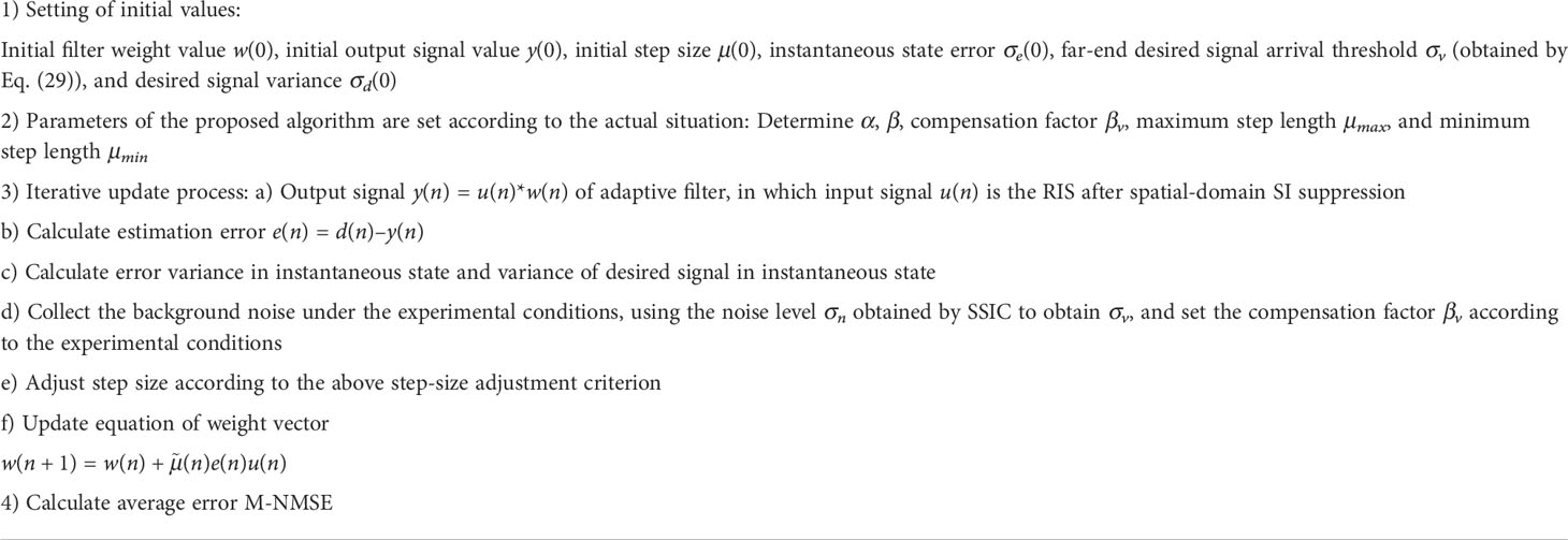
Table 1 Specific flow of the SNT-VSS-LMS algorithm.

Unlike the traditional VSS-LMS algorithm, we consider the influence of the arrival of the desired signal on the RIS channel estimation process. The SNT-VSS-LMS algorithm adaptively adjusts the step size by examining the relationship between σ_e(n) and σ_v,γ_vσ_d in the convergence process according to Eq. (28), i.e., when σ_e(n) is less than σ_v , the main error of the SI channel estimation process depends on the desired signal, so the step size is reduced to μ_min  ; when σ_e(n) is greater than γ_vσ_d , the main error of the SI channel estimation process depends on the RIS and the step size is adjusted to μ_max  for faster convergence. When σ_e(n) is in the intermediate state, the step is constrained using the parabolic function. In this way, the SNT-VSS-LMS algorithm obtains better steady-state results and faster convergence. Compared with the traditional VSSLMS algorithm, our proposed algorithm determines the step value referring to the SI signal after SSIC, which can minimize the impact of the desired signal while ensuring the convergence speed and steady-state effect.

Figure 2 shows a flowchart of the proposed SDSIC method. After SSIC, the RIS is subjected to DSIC to complete the SIC process, resulting in the distant desired signal to be demodulated.

FIGURE 2

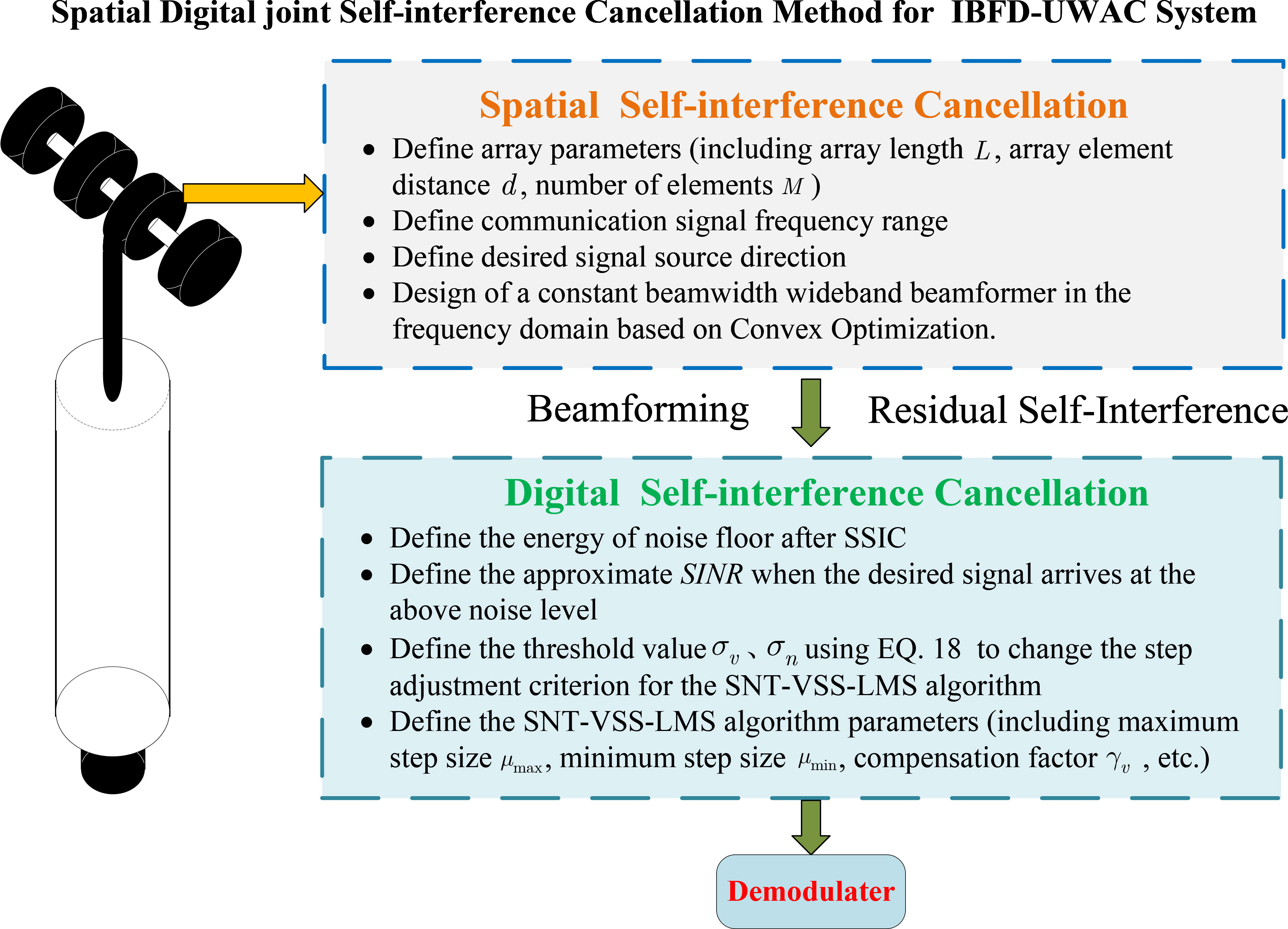
Figure 2 Flowchart of the SDSIC method.

To evaluate the performance of our proposed algorithm, we examine the results of simulations and experiments in the next section.

4 Simulation analysis

4.1 SSIC simulation

To illustrate the SIC effect and the signal restoration effect, the simulation experiments use a high-power single-frequency SI signal. The desired signal is an LFM signal. To make the experimental scenario closer to that of engineering applications, the SI signal and the desired signal overlap. We collected simulation data from an anechoic pool. The frequency of the SI signal is 4 kHz, and the LFM frequency range is 3–5 kHz. The direction of the signal is 70°, the number of array elements is M=12 , and the distance between each array element is d=0.185 m.

Figure 3 shows the beam response of the beamformer with the minimum variance distortion less response (MVDR)-MAILLOUX algorithm (Mailloux, 1995). This algorithm uses the MVDR with some virtual interference sources in a preset angle range to accomplish a more extensive range of zero trapping. The MVDR-MAILLOUX beamformer achieves excellent cancellation from 65–75°, but the beam responses are significantly different at each frequency point around the desired direction of 0°, and the lowest frequency point of the main flap widths is 19.5°. The maximum frequency distortion reaches 4.2 dB in the range [-5°, 5°]. In actual applications, the array will drift due to waves and other environmental factors, and the position is not fixed. Thus, the guiding vector will be mismatched, and there will be frequency distortion when the signal is restored. This will result in a loss of frequency characteristics from the far-end desired signal after restoration, which will have a specific impact on the BER performance of the communication system. To solve this problem, it is necessary to make the spectrum of the base array signal distortion less after passing through the beamformer, and the beam response of each frequency point should be the same. As the beamformer should have approximately the same primary flap beam response at each frequency point, the “constant-beamwidth” beamformer is of considerable interest (Krolik and Swingler, 1990).

FIGURE 3

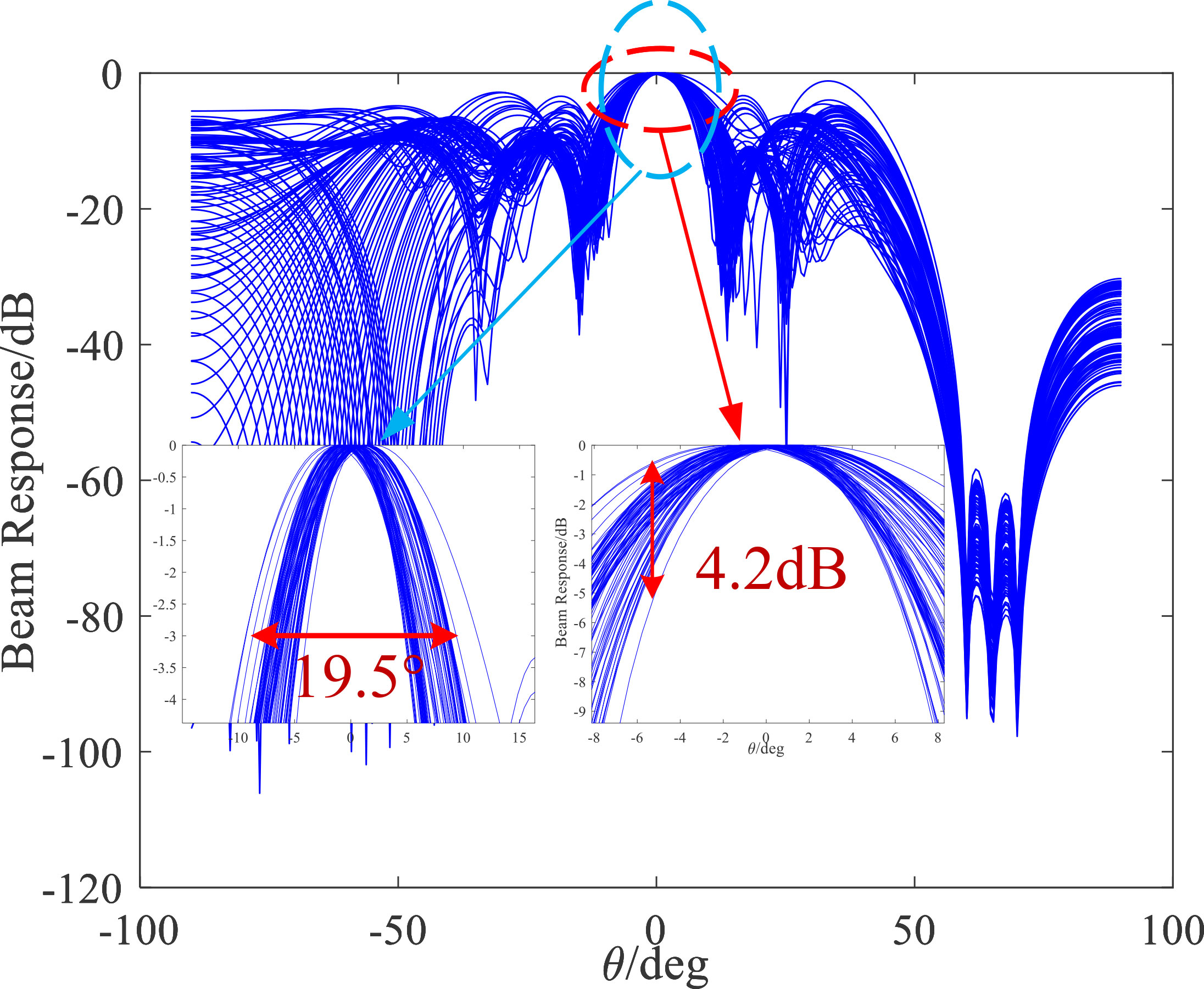
Figure 3 Beam response of the MVDR-MAILLOUX beamformer.

Figure 4 shows the beam response of the adaptive beamformer based on the LMS algorithm. We can see that the main flap width of the lowest frequency point response of the beamformer optimized by the LMS adaptive algorithm is 19°. The maximum value of the primary flap frequency distortion is 2.9 dB in the range [-5°, 5°]. The constant-beamwidth beamformer exhibits an excellent ability to restore the signal. However, the amplitude of the array drift is large, and the beam response needs to be kept consistent within a specific angle range.

FIGURE 4

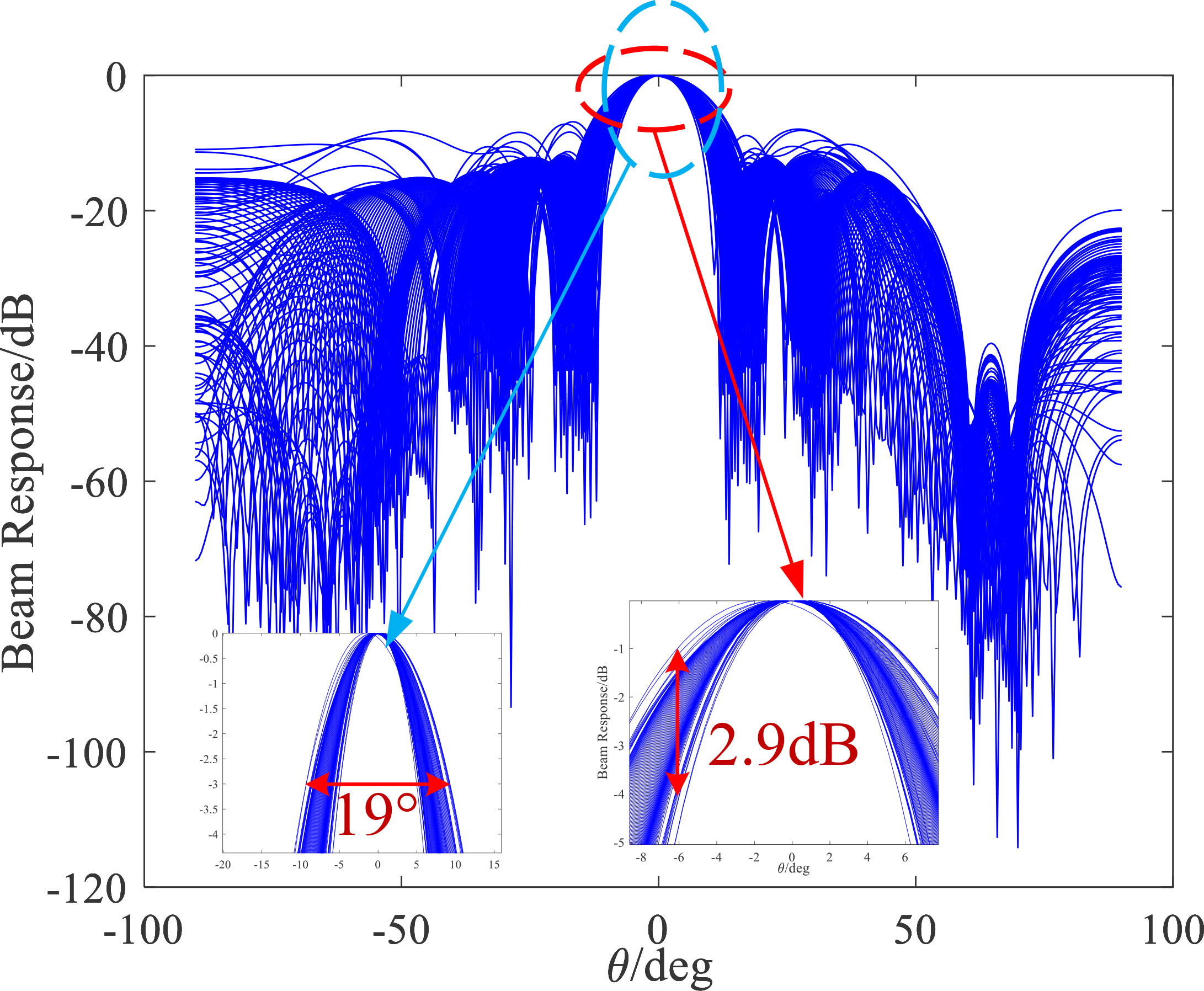
Figure 4 Beam response of the adaptive beamformer based on LMS algorithm.

Figure 5 shows the beam response of the constant-beamwidth beamformer based on Newton’s iteration method. The maximum frequency distortion is 0.4 dB in the range [-5°, 5°] and 2 dB in the range [-10°, 10°]. The beam response of this method controls the main flap within a specific range, which solves the problem of array drift, i.e., the mismatch of the guiding vector.

FIGURE 5

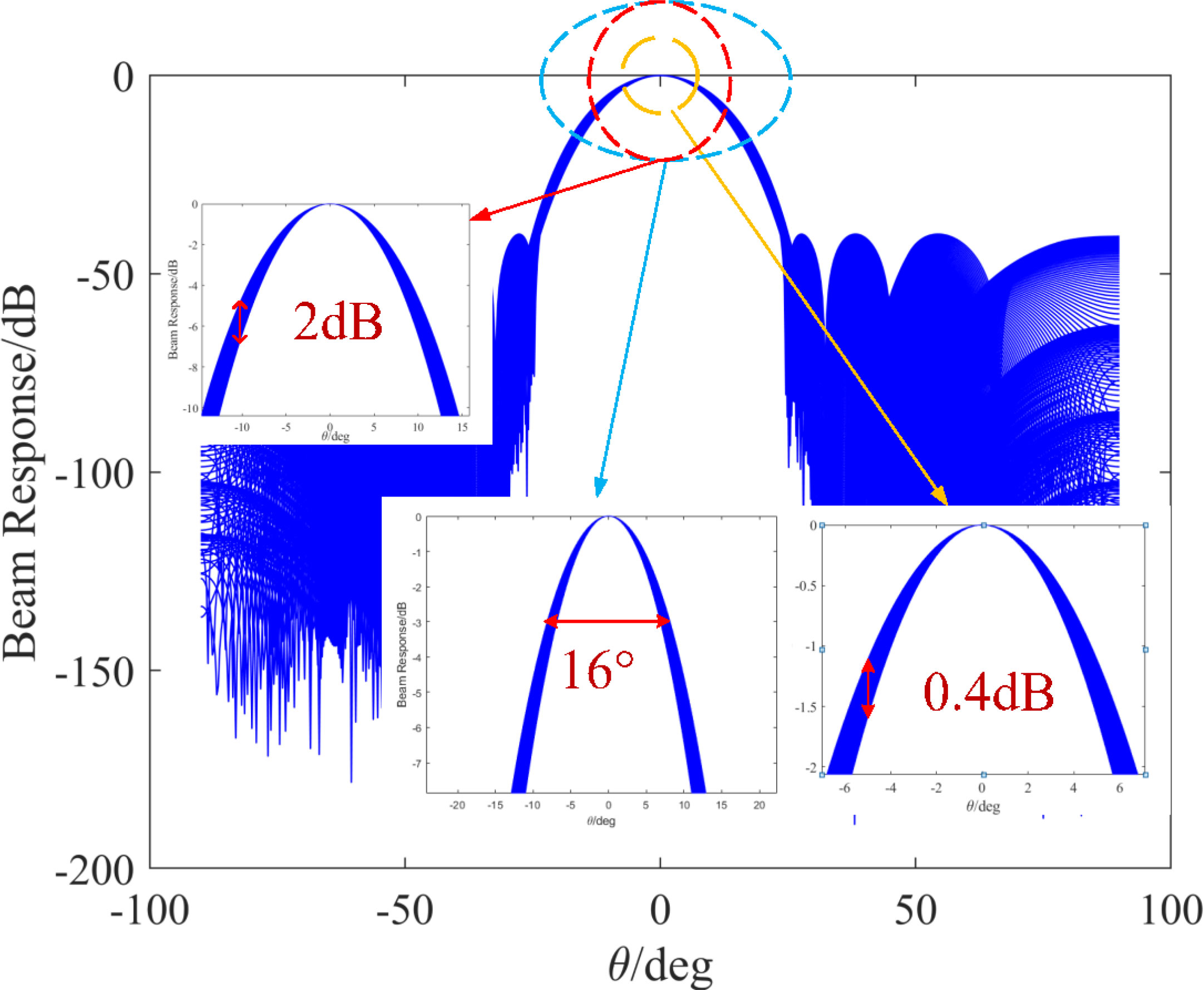
Figure 5 Beam response of the constant-beamwidth beamformer based on Newtonian iteration.

However, the beam response of this beamformer is below -40 dB for the rest of the side flaps beside the interference source, and the width of the main flap is too large. Additionally, the beamformer’s angle resolution decreases. The simulation results of the proposed SSIC method are given below. According to the experimental data, the parameters of the convex optimization process described in Section 3.1 are set as follows: θ_MF=[−5°,5°] , θ_SF=[−90^¸irc,−8°]∪[8°,90°] , θ_ZF=[65°,75°] . In the simulation, ξ_SF=10^−15/20 , ξ_ZF=10^−60/20 , and θ_d=0° is the desired signal source direction. After solving the convex optimization problem, the obtained beam response is shown in Figure 6. The main flap width of the lowest frequency point response of the proposed method is 10°, and the maximum frequency distortion in the range [-5°, 5°] is 1.9 dB, and so the main flap width has been reduced by achieving a consistent main flap beam response and the beamformer’s resolution has been enhanced. Moreover, the beamformer cancels signals around the 70° direction and preserves signals from other directions, which is of great significance for constructing a full-duplex UWAC network. In subsequent simulations, we performed the SSIC process with the ICBBF based on convex optimization.

FIGURE 6

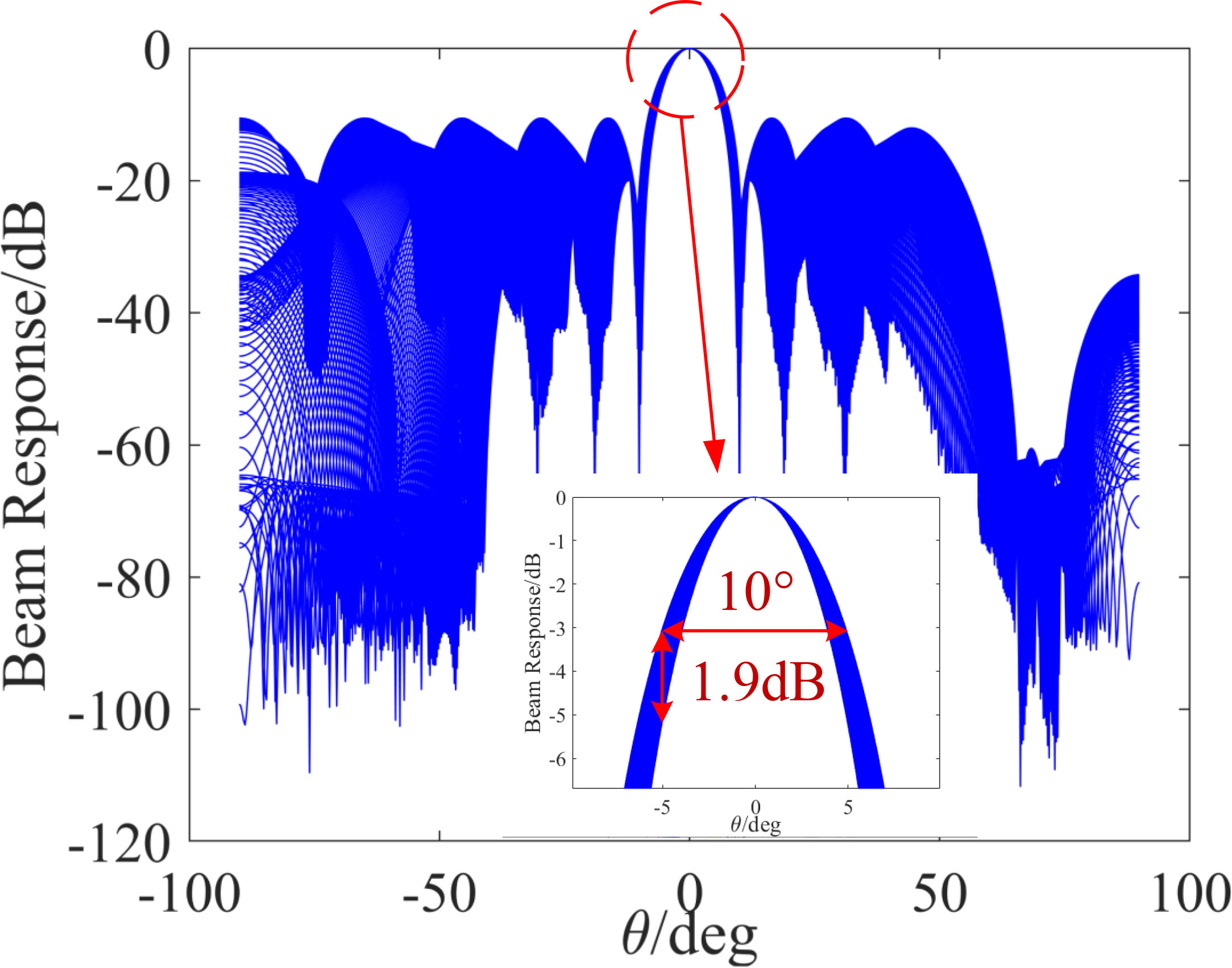
Figure 6 Spectrum of the signal after the constant-beamwidth beamformer based on Newtonian iteration.

In the SSIC simulation experiments, the distance between each array element was set to 0.185 m, the number of array elements was fixed at 12, and the sampling frequency was 50 kHz. The desired signal had a direction of 0° and the SI signal had a direction of 70°. Note that, because the beamformer weights the data of each array element to obtain the new data, we compared the far-end desired signal with the SI signal after the beamformer. To determine the SIC effect, the non-overlapping part of the signal was used to calculate the cancellation effect:

$\begin{array}{ll}\begin{array}{l}{\zeta }_{\text{BF}}=10\times \lg ({\sigma }_1^2/{\sigma }_2^2)-10\times \lg ({\sigma }_3^2/{\sigma }_4^2)\hfill \end{array}& (30)\end{array}$

where σ₁ is the standard deviation of the non-overlapping part of the desired signal after beamforming, σ₂ is the standard deviation of the non-overlapping part of the desired signal from the reference array, σ₃ is the standard deviation of the non-overlapping part of the SI signal after beamforming, and σ₄ is the standard deviation of the non-overlapping part of the SI signal from the reference array.

The purpose of the above equation is to keep the amplitude of the non-overlapping part of the desired signal consistent before and after beamforming. Figure 7 shows the normalized spectrum of the signal after SSIC and the signal received by the reference array.

FIGURE 7

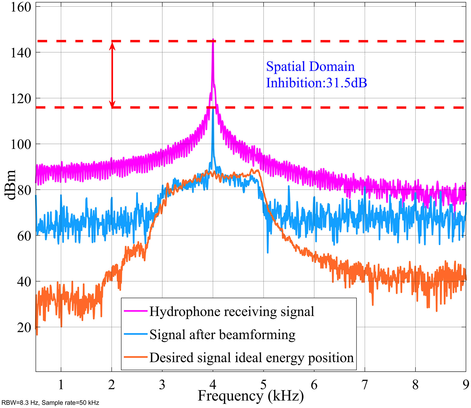
Figure 7 Spectrum of the signal after SSIC (after normalization).

The simulation results show that the SI signal is cancelled by 31.5 dB after SSIC. Next, the RIS was subjected to DSIC.

4.2 DSIC for RIS

In the DSIC simulation experiments, the local SI signal and the desired signal were wideband LFM signals. For the VSS-LMS algorithm, we set c=0.003 ; for the SNT-VSS-LMS algorithm, γ_v=0.8 , μ_max =0.003 , μ_min =0.0005 . The SNT-VSS-LMS algorithm obtains ${\sigma }_v=\sqrt{{\sigma }_n^2·{10}^{\frac{20}{10}}}$ with SINR_known=20 dB, and the SNR of the SI signal is SNR_SI=30 dB. Therefore, the step size starts to decrease, and when the NMSE reaches -10 dB, the step size is adjusted to the minimum μ_min =0.0005 . As can be seen, the SNT-VSS-LMS algorithm starts to reduce the step size before the cancellation is complete, preventing “over-cancellation” of the SI signal and reducing the influence of the desired signal on the filter steady state. To better demonstrate the superiority of the SNT-VSS-LMS algorithm, we simulated the case in which the desired signal completely overlaps with the SI signal. The NMSE curves are shown in Figure 8.

FIGURE 8

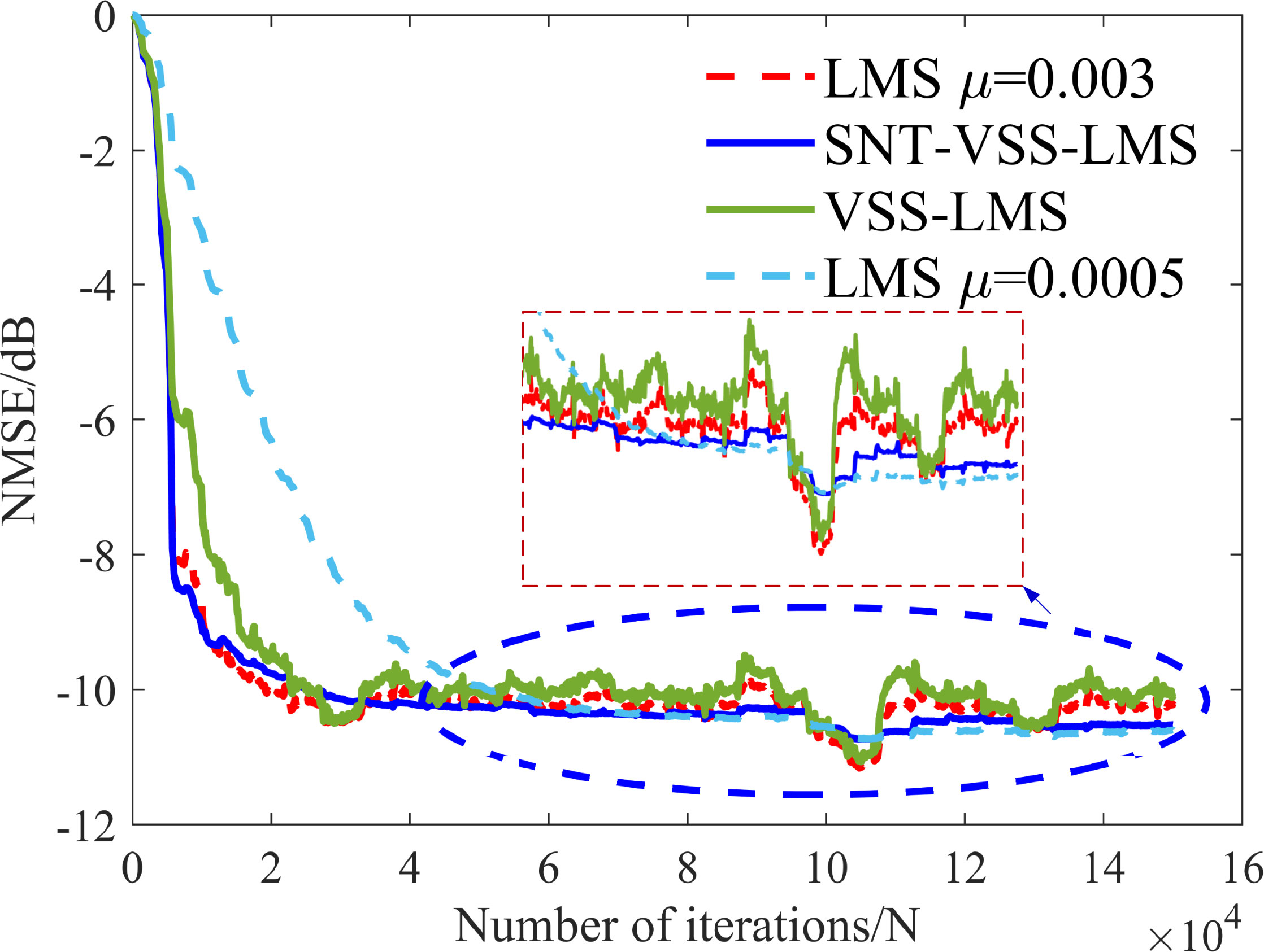
Figure 8 NMSE curves of DSIC using various algorithms.

Figure 8 shows the NMSE curves for DSIC using the SNT-VSS-LMS, VSS-LMS, and LMS algorithms in the case of an overlap between the desired signal and the SI signal. The SNT-VSS-LMS algorithm produces the best results when the filter cancellation is close to the steady-state and the fastest convergence rate for the cancellation iterations in the initial stages when the SI signal energy is high. We also show the BER under different interference-to-signal ratios (ISRs) in Figure 9 to illustrate the effect of SIC. The simulation analysis of the BER under a 10-dB SNR is carried out below. The ISR varies in the range [12, 22], and the BER is obtained at 2-dB intervals.

FIGURE 9

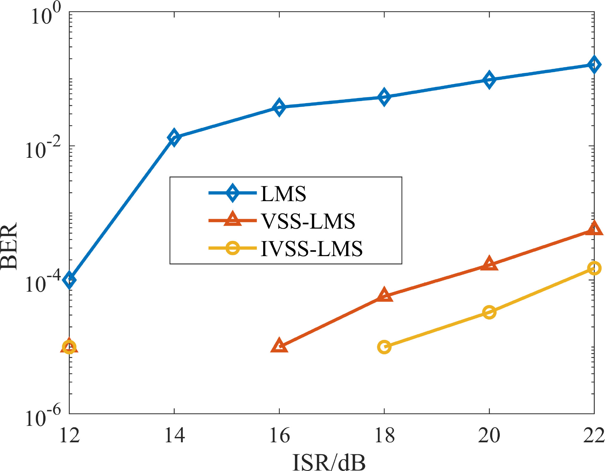
Figure 9 BER in simulations.

Figure 9 compares the BER performance of the three schemes under an SNR of 10 dB. As most of the RIS in the iterative process overlaps with the desired signal in the simulation considered in this paper, the LMS algorithm has a slow convergence speed. Indeed, the convergence time is longer than the desired signal arrival time, so demodulation without complete cancellation will significantly reduce the BER performance. The VSS-LMS and SNT-VSS-LMS algorithms achieve good BER performance because of the faster convergence speed. Although VSS-LMS has a reasonable convergence speed, it cannot adaptively judge the relationship between the RIS energy and the desired signal, resulting in poor steady-state performance and high BER. When the ISR is above a certain threshold, the BER increases with increasing ISR. This is because the energy of the SI signal increases, and when the ISR is less than a certain threshold, the BER increases instead. When the ISR is small, the desired signal worsens the filter steady state, this decreasing the BER.

5. Anechoic pool experiment

To prevent multipath effects from creating uncertainty in the direction of the signal source, the experiments were performed in an anechoic pool. The results are shown in Figure 10.

FIGURE 10

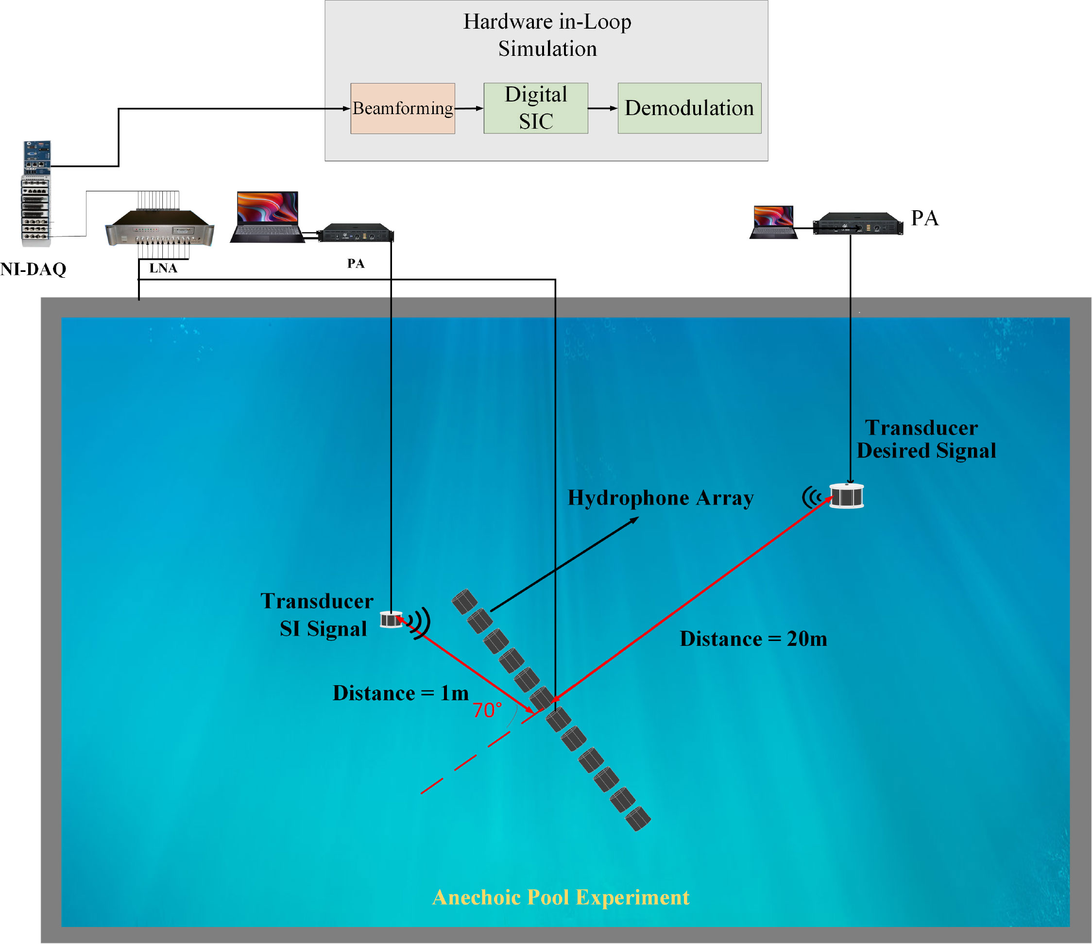
Figure 10 Schematic diagram of the experimental scenario.

The simulations were implemented in the Simulink ^® platform based on a hardware-in-the-loop framework, where the real-time implementation of the IBFD-UWAC system has more practical application value. In the experiments, the array element spacing was 0.185 m, the number of array elements was fixed to 12, and the sampling frequency was 50 kHz. The desired signal source had a direction of 0° and the SI signal had a direction of 70°.

The locally transmitted signal was an LFM signal plus Gaussian white noise, and the far-end desired signal at a distance of 20 m was an LFM signal. The aim of this experiment was to verify the cancellation effect of the proposed SDSIC method. The ICBBF described in Section 3.1 was used to cancel the SI signal at 70° degrees and enhance the desired signal at 0°.

Figure 11 compares the cancellation effects of the SDSIC and traditional SIC methods. The right side of Figure 11 shows a time-frequency diagram of the signal after the SDSIC method and the signal without SIC. In general, SSIC reduces the burden of SIC in the analog and digital domains and improves the upper limit of SIC under the same hardware conditions. This figure shows that using the traditional SIC scheme can cancel up to 36.2 dB of the SI signal, whereas the proposed SDSIC method can cancel up to 56.4 dB. The scheme and algorithm proposed in this paper are therefore highly effective. In a second experiment, the local transmitting signal was a 3–5 kHz LFM signal, and the far-end desired signal at a distance of 20 m was a direct-sequence spread spectrum signal in the same frequency band. This experiment was conducted to verify the cancellation effect of the proposed SDSIC method. Note that, in the IBFD-UWAC system, the SIC process takes a certain amount of time, and the two sides can communicate stably only after the SI signal has been canceled to a certain degree. Compared with the DSIC method, the SDSIC method first filters the received signal in the spatial domain, which reduces the width of the main flap while achieving a consistent main flap beam response, and accurately cancels the signal in the set direction (θ_ZF = [65°,75°]). This improves the resolution of the beamformer. The parameters of the signals in this experiment are listed in Table 2.

FIGURE 11

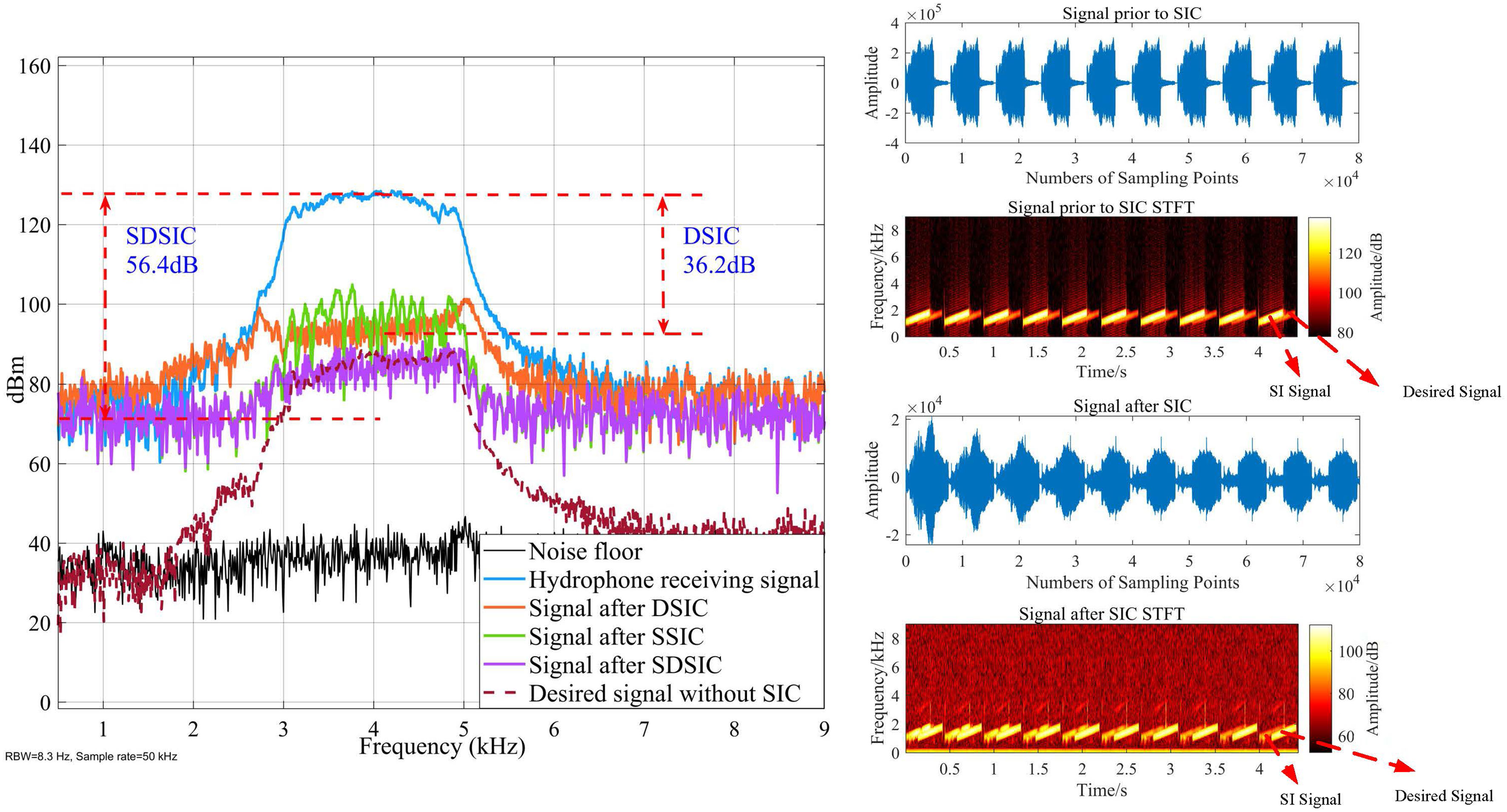
Figure 11 Comparison of cancellation effects between SDSIC method and traditional DSIC method.

TABLE 2

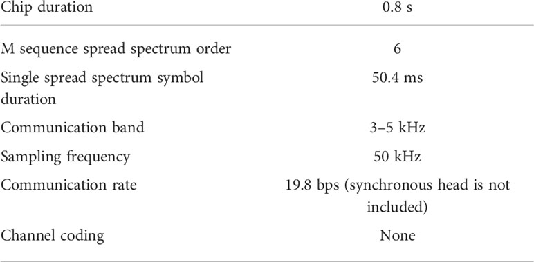
Table 2 Parameters of the spread spectrum communication signal.

As shown in Figure 12, both SDSIC and DSIC reach a steady state, although the SDSIC method has a better cancellation effect. The right side of Figure 12 shows a time-frequency diagram of the signal after the SDSIC method and the signal without SIC. The SSIC effect reaches 20 dB, and the SNR of the canceled signal SNR_RIS = 27 dB. The noise energy of the current signal ${\sigma }_n^2$ is obtained from the RIS, and the expected SINR of the desired signal SINR_known = 18 dB. The DSIC of the RIS was completed by the SNT-VSS-LMS algorithm using the step-size adjustment criterion of Eq. (28), and the expected threshold value based on the spatial domain noise σ_v was obtained from Eq. (29). We set c = 0.005 in the VSS-LMS algorithm and γ_v = 0.8, μ_max = 0.005, μ_min = 0.0001 in the SNT-VSS-LMS algorithm. The NMSE curves obtained from the RIS after applying the LMS, VSS-LMS, and SNT-VSS-LMS algorithms are shown in Figure 13.

FIGURE 12

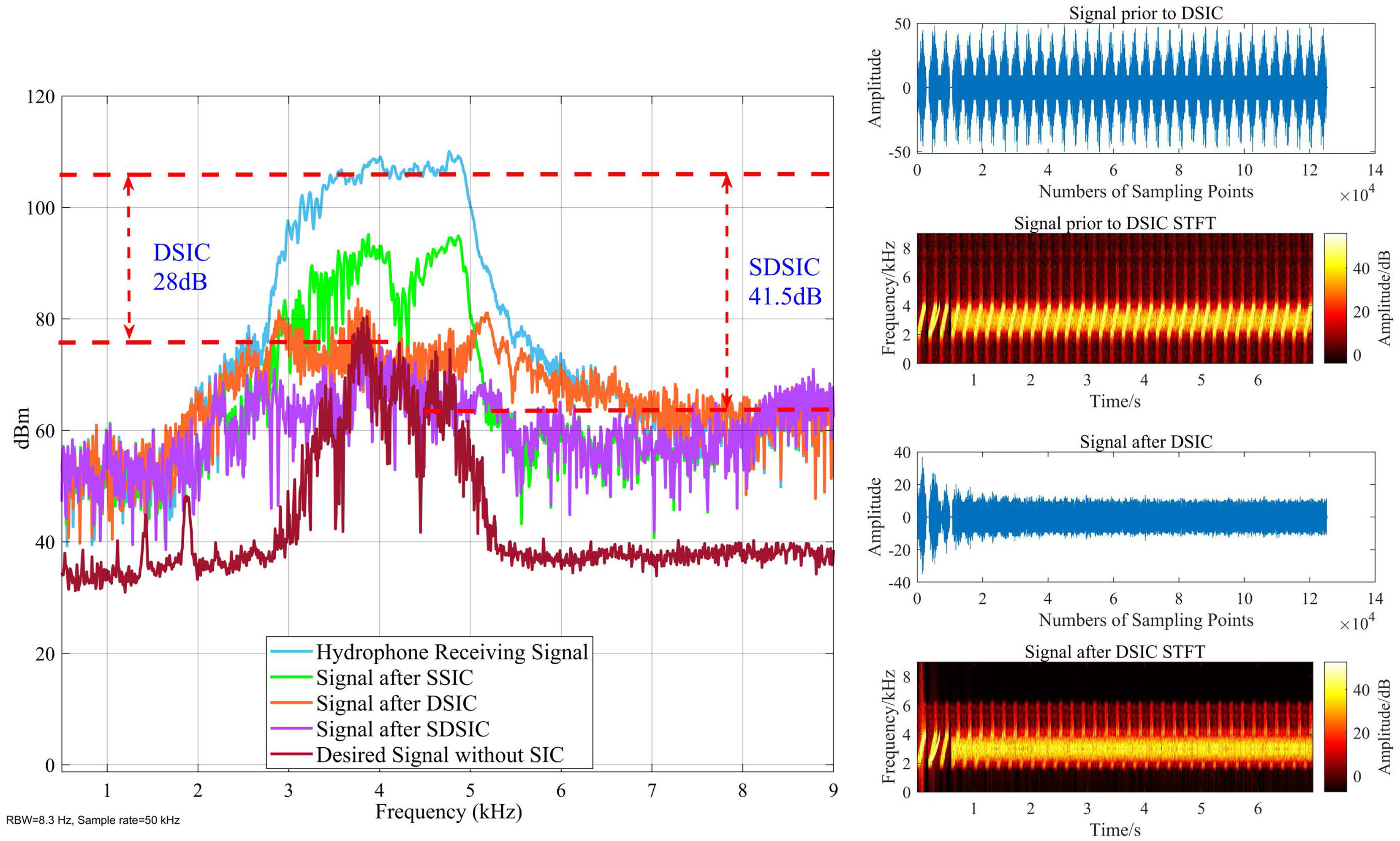
Figure 12 Cancellation effect of SDSIC method and traditional DSIC method.

FIGURE 13

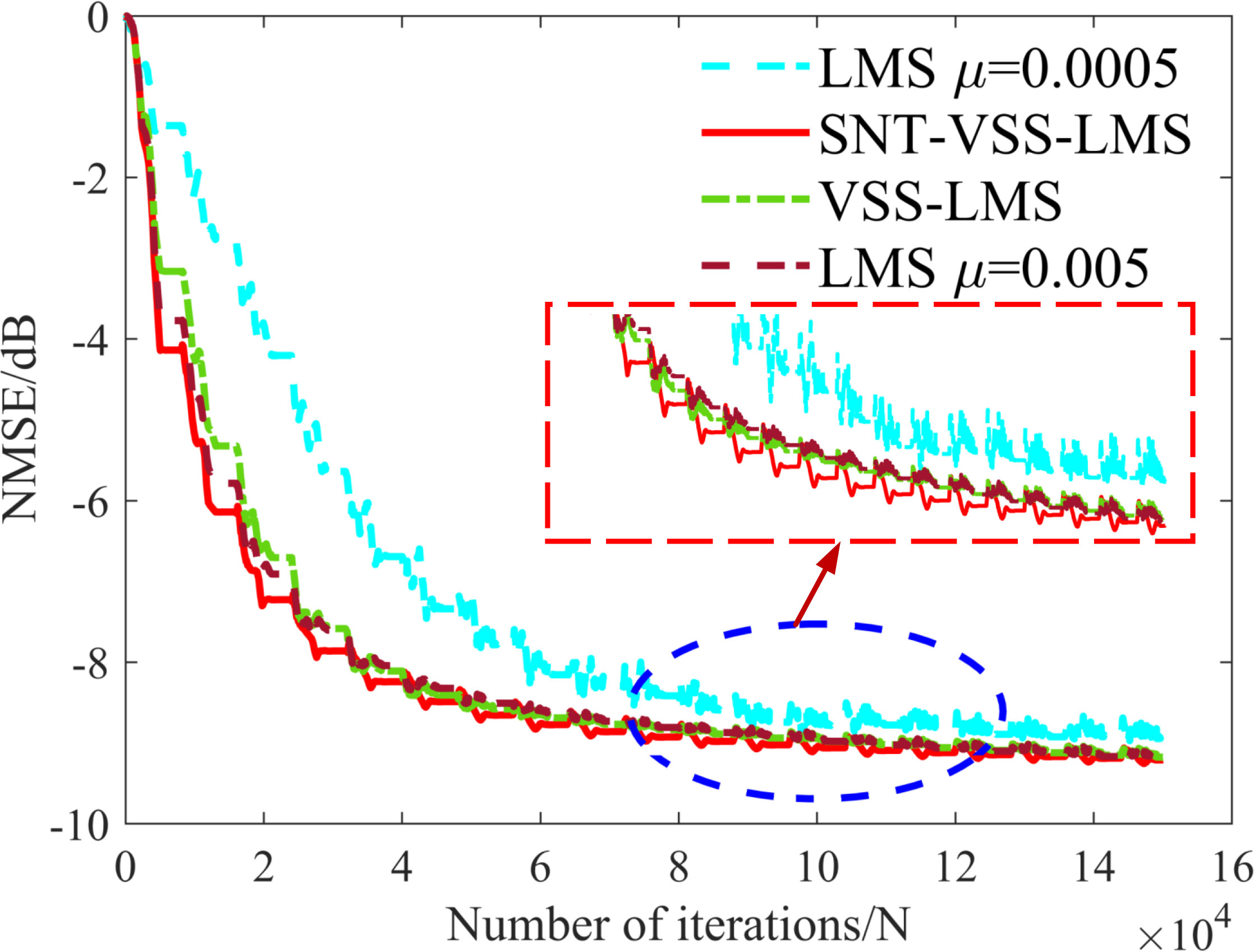
Figure 13 Comparison of cancellation performance between LMS, VSS-LMS, and SNT-VSS-LMS.

The SNT-VSS-LMS algorithm proposed in this paper has the fastest convergence speed, and the best steady-state effect after applying the DSIC process to the RIS. This algorithm can adjust the step size in real time according to the variance of the instantaneous state error. At first, the step size is set to 0.005 to achieve the fastest convergence speed when the SI signal is canceled by 24 dB (i.e., the NMSE result of the signal is close to SNR_SI–SINR_known = 9 dB), and then the step size is adjusted to prevent the SI signal from being over-canceled, which ensures the best steady-state effect. Figure 13 verifies the effectiveness of the algorithm and its superior performance compared with the VSS-LMS algorithm. The VSS-LMS technique gives a poorer steady-state effect because of its inability to determine adaptively where the desired signal is coming from and lack of optimization of the convergence speed. In summary, the proposed SNT-VSS-LMS algorithm produces an excellent DSIC effect for the RIS.

Next, we consider the BER performance of the IBFD-UWAC system. Note that, during the anechoic pool trial, the PA of the far-end transmitting ship was kept at its maximum value. When the two sides communicate, the arrival time of the far-end desired signal is not known, so the SIC algorithm requires a fast offset speed to ensure that the communication information is not lost. We now illustrate the offset effect of each SIC method under the different arrival times of the desired signal. In the communication experiment, we transmitted the SI signal locally without interruption, the desired signal was transmitted randomly, and we selected the data with different desired signal arrival times for subsequent processing to obtain the BER curve with respect to time. The results are shown in Figure 14, where t in the BER curve is the time from the start of the SIC process.

FIGURE 14

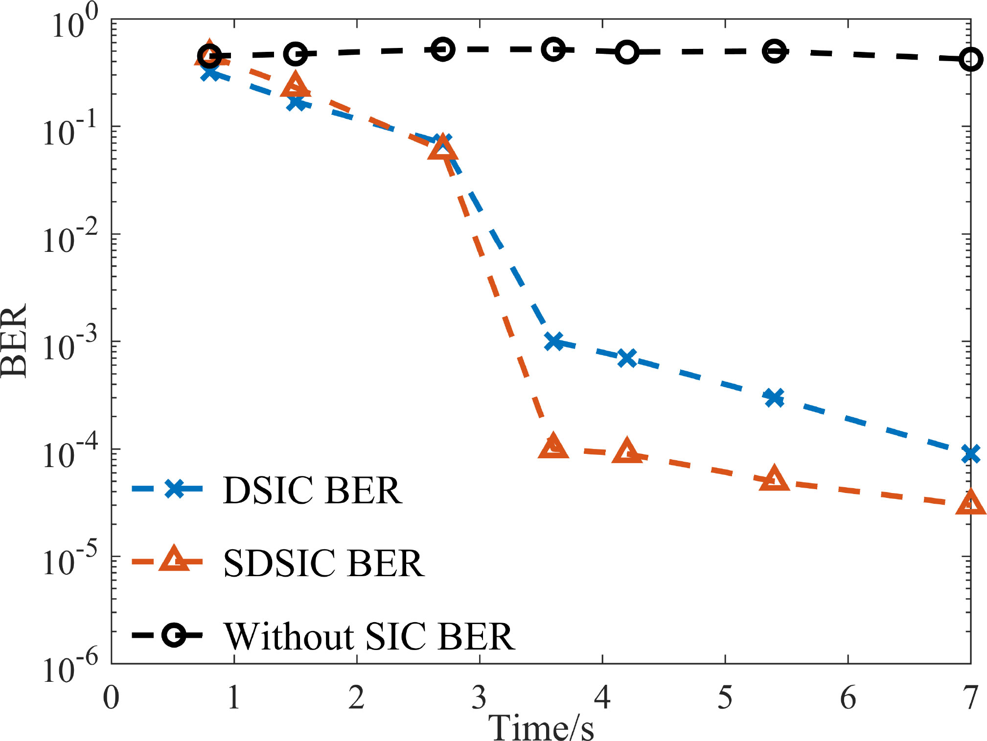
Figure 14 BER versus number of iterations for DSIC, SDSIC, and signal without SIC.

From Figure 14, a slower arrival of the desired signal results in a lower BER, because the SIC process takes some time. The proposed SDSIC significantly improves the BER performance after 2 s, but we cannot complete the communication before 2 s because the SSIC process also takes some time. When the desired signal arrives slowly, both SDSIC and DSIC have BERs of less than 10^-3 after offset, but SDSIC achieves better BER performance. Moreover, SDSIC has a faster SIC speed when the desired signal arrives early.

6. Conclusion

This paper has described a new SIC method for the unique problems of IBFD-UWAC systems. The proposed SDSIC method, including an SSIC method that is applicable to the IBFD-UWAC, uses a beamformer based on convex optimization theory to cancel the SI signal accurately, and can ensure perfect restoration of the distant desired signal. In addition, for the RIS after SSIC, we have proposed an SNT-VSS-LMS algorithm that modifies the step-size adjustment criterion of the traditional VSS-LMS algorithm. This algorithm initially cancels most of the RIS with a rapid convergence rate, and then sets the expected threshold based on the noise floor of the RIS and the SINR under which the far-end desired signal satisfies the performance condition of the communication BER. The expected threshold value of the DSIC process is intended to minimize the impact of the desired signal for the SI channel estimation process, resulting in a smaller mean square error and the optimal steady state. An experimental verification of the proposed SDSIC method was conducted in an anechoic pool using an IBFD-UWAC system. The traditional SIC method can cancel up to 28 dB of the SI signal, while the SDSIC method proposed in this paper cancels up to 41.5 dB, significantly improving the upper limit of SIC in IBFD-UWAC systems. In addition, the proposed SNT-VSS-LMS algorithm performs optimally in terms of both convergence speed and steady-state effect. The anechoic pool experiments verify the real-time effectiveness of the proposed method. The algorithm proposed in this paper is easy to implement and has low complexity, allowing it to be implemented in engineering applications. The proposed algorithm could be directly ported to a field-programmable gate array, with toolboxes such as HDL Coder in MATLAB^® used to realize the production of engineering prototypes.

Future work will investigate analog-domain SIC. Previous studies suggest that analog-domain SIC will be limited by the parameters of hardware circuits, e.g., PA, ADC sampling accuracy. Further research should investigate strong analog-domain SIC methods and attempt to combine them with SSIC methods. In this paper, DSIC was applied to the RIS signal after SSIC, and the experiments were performed in an anechoic pool. For environments with complex channels (e.g., marine environment), the published literature shows that the convergence process of LMS filters under fast time-varying channels can have a serious impact on the demodulation of information corresponding to the time variation. Thus, it would be worthwhile investigating an efficient DSIC scheme under fast time-varying channels.

Finally, the balanced relationship between analog-domain SIC and SSIC/DSIC should be considered, and the channel characteristics in the context of engineering applications should be further investigated to obtain the best SIC performance.

Data availability statement

The original contributions presented in the study are included in the article/supplementary material. Further inquiries can be directed to the corresponding author.

Author contributions

YL, CY, and YZ contributed to the conception and design of the study. GQ organized the database. YL and XQ performed the statistical analysis. YL and CY wrote the first draft of the manuscript. YL, CY, SW, and XQ wrote sections of the manuscript. All authors contributed to manuscript revision, and have read and approved the submitted version.

Funding

This work was supported by the Natural Science Foundation of Heilongjiang (Grant No. LH2021F010), Natural Science Foundation (Grant No. U1806201), Open Foundation of the Key Laboratory of Underwater Information and Control (Grant No. J2322048), and Open Foundation of Key Laboratory of Underwater Acoustic Countermeasure Technology (Grant No. JCKY2022207CH01).

Acknowledgments

The authors would like to thank all those who participated in the preparation of this paper, particularly the editors and reviewers.

Conflict of interest

The authors declare that the research was conducted in the absence of any commercial or financial relationships that could be construed as a potential conflict of interest.

Publisher’s note

All claims expressed in this article are solely those of the authors and do not necessarily represent those of their affiliated organizations, or those of the publisher, the editors and the reviewers. Any product that may be evaluated in this article, or claim that may be made by its manufacturer, is not guaranteed or endorsed by the publisher.

References

Ahmed E., Eltawil A. M. (2015). All-digital self-interference cancellation technique for full-duplex systems. IEEE Trans. Wirel. Commun. 14, 3519–3532. doi: 10.1109/TWC.2015.2407876

CrossRef Full Text | Google Scholar

Cacciola R., Holzman E., Carpenter L., Gagnon S. (2016). “Impact of transmit interference on receive sensitivity in a bi-static active array system,” in 2016 IEEE International Symposium on Phased Array Systems and Technology (PAST, IEEE), IEEE, Waltham, Massachusetts, USA Vol. 1–5. doi: 10.1109/ARRAY.2016.7832623

CrossRef Full Text | Google Scholar

Chan S. C., Chen H. H. (2007). Uniform concentric circular arrays with frequency-invariant characteristics–theory, design, adaptive beamforming and doa estimation. IEEE Trans. Signal Process. 55, 165–177. doi: 10.1109/TSP.2006.882109

CrossRef Full Text | Google Scholar

Choi J., Jain M., Srinivasan K., Levis P., Katti S. (2010). “Achieving single channel, full duplex wireless communication,” in Proceedings of the sixteenth annual international conference on Mobile computing and networking. Association for Computing Machinery, New York, United States 1–12. doi: 10.1145/1859995.1859997

CrossRef Full Text | Google Scholar

Everett E., Sahai A., Sabharwal A. (2014). Passive self-interference suppression for full-duplex infrastructure nodes. IEEE Trans. Wirel. Commun. 13, 680–694. doi: 10.1109/TWC.2013.010214.130226

CrossRef Full Text | Google Scholar

Everett E., Shepard C., Zhong L., Sabharwal A. (2016). Softnull: Many-antenna full-duplex wireless via digital beamforming. IEEE Trans. Wirel. Commun. 15, 8077–8092. doi: 10.1109/TWC.2016.2612625

CrossRef Full Text | Google Scholar

Fan Z., Liang G.-l. (2013). Broadband beamforming with minimum sidelobe and constant beamwidth based on convex optimization. Acta Electon. Sin. 41, 943. doi: 10.3969/j.issn.0372-2112.2013.05.018

CrossRef Full Text | Google Scholar

Goodwin M., Elko G. (1993). “Constant beamwidth beamforming,” in 1993 IEEE International Conference on Acoustics, Speech, and Signal Processing (ICASSP, IEEE, Minneapolis, MN, USA), Vol. 1. 169–172. doi: 10.1109/ICASSP.1993.319082

CrossRef Full Text | Google Scholar

Kolodziej K. E., Perry B. T., Herd J. S. (2019). In-band full-duplex technology: Techniques and systems survey. IEEE Trans. Microw. Theory Tech. 67, 3025–3041. doi: 10.1109/TMTT.2019.2896561

CrossRef Full Text | Google Scholar

Krolik J., Swingler D. (1990). Focused wide-band array processing by spatial resampling. IEEE Trans. Acoust. Speech Signal Process. 38, 356–360. doi: 10.1109/29.103073

CrossRef Full Text | Google Scholar

Li L., Song A., Cimini L. J., Xia X.-g., Shen C.-C. (2015). “Interference cancellation in in-band full-duplex underwater acoustic systems,” in OCEANS 2015 - MTS/IEEE Washington. (IEEE, Washington, DC, USA) 1–6. doi: 10.23919/OCEANS.2015.7404411

CrossRef Full Text | Google Scholar

Liu R., Cui G., Lu Q., Yu X., Feng L., Zhu J. (2021). “Constant beamwidth receiving beamforming based on template matching,” in 2021 IEEE Radar Conference (RadarConf21). (IEEE, Atlanta, GA, USA) 1–5. doi: 10.1109/RadarConf2147009.2021.9455192

CrossRef Full Text | Google Scholar

Liu J., Lee J., Li L., Luo Z.-Q., Wong K. (2005). Online clustering algorithms for radar emitter classification. IEEE Trans. Pattern Anal. Mach. Intell. 27, 1185–1196. doi: 10.1109/TPAMI.2005.166

PubMed Abstract | CrossRef Full Text | Google Scholar

Liu W., Weiss S. (2008). Design of frequency invariant beamformers for broadband arrays. IEEE Trans. Signal Process. 56, 855–860. doi: 10.1109/TSP.2007.907872

CrossRef Full Text | Google Scholar

Liu W., Weiss S., Mcwhirter J., Proudler I. (2007). Frequency invariant beamforming for two-dimensional and three-dimensional arrays. Signal Process. 87, 2535–2543. doi: 10.1016/j.sigpro.2007.03.018

CrossRef Full Text | Google Scholar

Liu J., Zakharov Y. V., Weaver B. (2009). Architecture and fpga design of dichotomous coordinate descent algorithms. IEEE Trans. Circ. Syst. I: Reg. Pap. 56, 2425–2438. doi: 10.1109/TCSI.2009.2015725

CrossRef Full Text | Google Scholar

Li S., Yang X., Ning L., Long T., Sarkar T. K. (2017). “Broadband constant beamwidth beamforming for suppressing mainlobe and sidelobe interferences,” in 2017 IEEE Radar Conference (RadarConf). (RadarConf, IEEE, Seattle, USA) 1041–1045. doi: 10.1109/RADAR.2017.7944358

CrossRef Full Text | Google Scholar

Mailloux R. (1995). “Covariance matrix augmentation to produce adaptive array pattern troughs,” in IEEE Antennas and Propagation Society International Symposium, (IEEE, Newport Beach, CA, USA) Vol. 1. 102–105 (1995 Digest (IEEE). doi: 10.1109/APS.1995.529973

CrossRef Full Text | Google Scholar

Makar G., Tran N., Karacolak T. (2017). A high-isolation monopole array with ring hybrid feeding structure for in-band full-duplex systems. IEEE Antennas Wirel. Propag. Lett. 16, 356–359. doi: 10.1109/LAWP.2016.2577003

CrossRef Full Text | Google Scholar

Nawaz H., Tekin I. (2016). “Three dual polarized 2.4ghz microstrip patch antennas for active antenna and in-band full duplex applications,” in 2016 16th Mediterranean Microwave Symposium (MMS). (IEEE, Abu Dhabi, United Arab Emirates) 1–4. doi: 10.1109/MMS.2016.7803854

CrossRef Full Text | Google Scholar

Pan C., Jia L., Cai R., Ding Y. (2012). Modeling and simulation of channel for underwater communication network. Int. J. innov. comput. Inf. control: IJICIC, 2149–2156.

Google Scholar

Qiao G., Gan S., Liu S., Ma L., Sun Z. (2018a). Digital self-interference cancellation for asynchronous in-band full-duplex underwater acoustic communication. Sensors 18, 1700. doi: 10.3390/s18061700

CrossRef Full Text | Google Scholar

Qiao G., Gan S., Liu S., Song Q. (2018b). Self-interference channel estimation algorithm based on maximum-likelihood estimator in in-band full-duplex underwater acoustic communication system. IEEE Access 6, 62324–62334. doi: 10.1109/ACCESS.2018.2875916

CrossRef Full Text | Google Scholar

Qiao G., Liu S., Sun Z., Zhou F. (2013). “Full-duplex, multi-user and parameter reconfigurable underwater acoustic communication modem,” in 2013 OCEANS - San Diego (IEEE). (IEEE, San Diego, CA, USA) 1-8. doi: 10.23919/OCEANS.2013.6741096

CrossRef Full Text | Google Scholar

Roe J., Cussons S., Feltham A. (1990). Knowledge-based signal processing for radar esm systems. IEEE Proc. Part F. Commun. radar Signal Process. 137, 293–301. doi: 10.1049/ip-f-2.1990.0045

CrossRef Full Text | Google Scholar

Sabharwal A., Schniter P., Guo D., Bliss D. W., Rangarajan S., Wichman R. (2014). In-band full-duplex wireless: Challenges and opportunities. IEEE J. Sel. Area. Commun. 32, 1637–1652. doi: 10.1109/JSAC.2014.2330193

CrossRef Full Text | Google Scholar

Satyanarayana K., El-Hajjar M., Kuo P.-H., Mourad A., Hanzo L. (2019). Hybrid beamforming design for full-duplex millimeter wave communication. IEEE Trans. Veh. Technol. 68, 1394–1404. doi: 10.1109/TVT.2018.2884049

CrossRef Full Text | Google Scholar

Shen L., Henson B., Zakharov Y., Mitchell P. (2020). Digital self-interference cancellation for full-duplex underwater acoustic systems. IEEE Trans. Circ. Syst. II: Express Briefs 67, 192–196. doi: 10.1109/TCSII.2019.2904391

CrossRef Full Text | Google Scholar

Snow T., Fulton C., Chappell W. J. (2011). Transmit–receive duplexing using digital beamforming system to cancel self-interference. IEEE Trans. Microw. Theory Tech. 59, 3494–3503. doi: 10.1109/TMTT.2011.2172625

CrossRef Full Text | Google Scholar

Song A., Stojanovic M., Chitre M. (2019). Editorial underwater acoustic communications: where we stand and what is next? IEEE J. Ocean. Eng. 44, 1–6. doi: 10.1109/JOE.2018.2883872

CrossRef Full Text | Google Scholar

Vallese P., Varanese N., Spagnolini U. (2017). “Self-interference cancellation for multi-antenna full duplex radio systems,” in WSA 2017; 21th International ITG Workshop on Smart Antennas. (IEEE, Berlin, Germany) 1–6.

Google Scholar

Yan H., Ma T., Pan C., Liu Y., Liu S. (2021). “Statistical analysis of time-varying channel for underwater acoustic communication and network,” in 2021 International Conference on Frontiers of Information Technology. (FIT, IEEE, Greenville, SC, USA) 55–60.

Google Scholar

Yin Y. L. (2016). Multi-carrier communication and cross-layer design of underwater acoustic communication network (Harbin Engineering University, Harbin).

Google Scholar

Zakharov Y. V., White G. P., Liu J. (2008). Low-complexity rls algorithms using dichotomous coordinate descent iterations. IEEE Trans. Signal Process. 56, 3150–3161. doi: 10.1109/TSP.2008.917874

CrossRef Full Text | Google Scholar

Zhang Z., Long K., Vasilakos A. V., Hanzo L. (2016). Full-duplex wireless communications: Challenges, solutions, and future research directions. Proc. IEEE 104, 1369–1409. doi: 10.1109/JPROC.2015.2497203

CrossRef Full Text | Google Scholar

Zhao Y. (2021). Research on key technology of self-interference cancellation in full duplex underwater acoustic communication (Harbin Engineering University, Harbin).

Google Scholar

Zhao Y., Qiao G., Liu S., Zakharov Y., Ahmed N. (2021). Self-interference channel modeling for in-band full-duplex underwater acoustic modem. Appl. Acoust. 175, 107687. doi: 10.1016/j.apacoust.2020.107687

CrossRef Full Text | Google Scholar