Application of interpolation methodology with dynamical constraint to the suspended particulate matter in the Liaodong Bay

Introduction: Suspended Particulate Matter (SPM) influences the primary production and the distributions of pollutants in the ocean. Besides, the regulation mechanisms of SPM in the Liaodong Bay were complicated.

Method: To analyze the distributions and influencing factors of SPM, based on the adjoint assimilation method, an interpolation method with dynamical constraint was established in the Liaodong Bay.

Result: In two ideal experiments, the cost function, Mean Absolute Error (MAE) and Normalized Mean Error (NME) all had reduced by more than 90%, which proved the accuracy of the interpolation method. Based on conventional observations of SPM, the distributions of dynamically constrained, Kriging and radial basis function (RBF) interpolations in March, May, August and October of 2015 were obtained.

Discussion: The cross-validation was carried out to compare the dynamically constrained interpolation and the unconstrained interpolations. Among seven unconstrained interpolation methods, the averaged MAE of RBF interpolation was the lowest, which was 10.976 mg/L. The averaged MAE of dynamically constrained interpolation was 7.703 mg/L, reduced by 29.8% compared with the RBF interpolation. It was indicated that RBF interpolation was the most accurate among the seven unconstrained interpolations and dynamically constrained interpolation was more accurate than unconstrained interpolations at the observation stations. The distributions of dynamically constrained and RBF interpolations were compared with Korean Geostationary Ocean Color Imager (GOCI) satellite-derived distributions of SPM concentrations in the Liaodong Bay. Fully considering the influences of the hydrodynamic processes, the dynamically constrained interpolation provided distributions more consistent with the satellite-derived distributions. However, due to the lack of observations in some areas and ignoring the influences of currents, some high values of SPM concentration were not captured by the distributions of RBF interpolation. Moreover, in accordance with the results of dynamically constrained interpolation, it was found that the SPM concentrations in the bay were affected by the SPM discharge from the Liao River Basin.

1. Introduction

Suspended Particulate Matter (SPM) has a profound impact on the biogeochemical processes in the ocean. The transport and transformation of nutrients in seawater are influenced by SPM (Volpe et al., 2011). Besides, SPM determines the optical indexes of seawater such as chroma and transparency. Hence, phytoplankton can be affected by SPM. It was found that phytoplankton productivity in turbid ocean areas was less than in the adjacent ocean (Cloern, 1987) and SPM concentration was negatively correlated with phytoplankton density (He et al., 2017) in previous studies. Therefore, the primary production in ocean is influenced by the distributions of SPM concentrations. During transferring along the currents, SPM adsorbs and releases the pollutants such as heavy metals, thereby effecting the distributions of marine pollutants. The pollutants can be transported from the coastal area to open sea along with SPM, and have potentially harmful effects on marine organisms (Yao et al., 2016). In addition, the sedimentation and resuspension processes of substances are also affected by SPM. These processes have an important impact on the coastal sea area (D’Sa et al., 2006).

The distributions of SPM in seawater are complicated and will be affected by many factors. Hydrodynamic processes will influence the distributions of SPM. Walker and Hammack (2000) found that strong northerly winds in winter could increase the concentration of SPM in the water column by five times in the northern Gulf of Mexico, and a large turbid plume was produced under the influence of wind-drive horizontal currents and resuspension. Estuarine discharge is a critical factor causing the variations of SPM distributions. Based on the remotely sensed data, Li et al. (2019) proved that due to the variations of SPM discharge from the Yellow River estuary, the SPM concentrations in Laizhou Bay and the southern Bohai Sea will be significantly higher in spring and winter than in summer and autumn. Moreover, the atmospheric deposition, the fragmentation process and the flocculation process in coastal systems can affect the concentration of SPM in seawater (Maerz et al., 2016; Xie et al., 2022; Fettweis et al., 2014). Therefore, it is necessary to study the distributions and the influencing factors of SPM in marine biogeochemical research.

The Bohai Sea is the largest inland sea in China (Figure 1A). The Liaodong Bay is one of the three most important bays of the Bohai Sea which is located in the northern part of the Bohai Sea (Figure 1B). The Liaodong Bay is surrounded by Hebei and Liaoning provinces on three sides. The line from Qinhuangdao of Hebei Province to Laotieshan Cape of Liaodong Peninsula is the boundary between the Liaodong Bay and the central area of the Bohai Sea (Lan et al., 2016). The estuary area (40.6°N-41.2°N, 121.5°E-122.2°E) is located in the northeast of the Liaodong Bay, including estuaries of Liaohe River, Daliao River and Daling River, which is the most important SPM source in the Liaodong Bay (Yan et al., 2020). As the second largest river in the Bohai Sea, the Liaohe River transports a high load of fine-grained sediments to the Liaodong Bay, which increases the SPM concentration in the bay (Jiang et al., 2004). In addition, the Yellow River discharges a large number of SPM every year. Under the influence of ocean currents, the water with high SPM concentration was transported into the Liaodong Bay through the central Bohai Sea from Laizhou Bay (Liu et al., 2007). The distributions of SPM in the Liaodong Bay are also influenced by the circulation. The detrital fine-grained sediments in the north of the Liaodong Bay were transported mainly via the surface currents (Dou et al., 2014). Moreover, the resuspension process also contributes to the formation of high SPM concentration in the Liaodong Bay (Jiang et al., 2004).

FIGURE 1

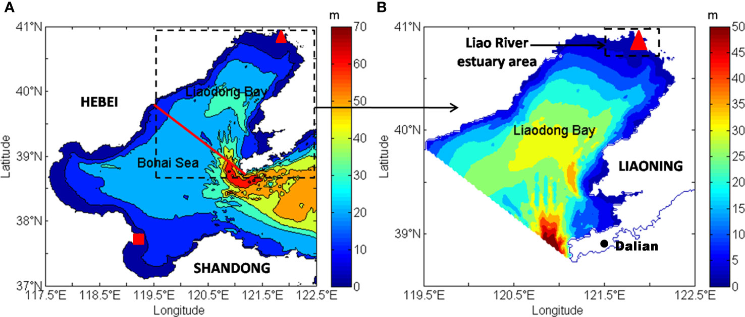
Figure 1 Geographical locations and bathymetry of the Bohai Sea and the Liaodong Bay. (A) shows the Bohai Sea, in which the red solid line is the boundary between the Liaodong Bay and the central Bohai Sea. The northwest end of the boundary is Qinhuangdao and the southeast end of the boundary is the Laotieshan Cape. The red triangle points out the estuary of the Liao River and the red square stands for the estuary of the Yellow River. The Liaodong Bay is selected using the black dotted line. (B) shows the study area, which is the Liaodong Bay. The red triangle still represents the estuary of the Liao River. The land on northwest side is Hebei Province and the land on the southeast side is Liaoning Province. Dalian city is located at the east of the mouth of the Liaodong Bay. The depth of the Liaodong Bay is deep in the central area and shallow around. The deepest region is near the mouth of the bay and the depth is more than 50m.

In order to study the spatial and temporal variations and regulation mechanisms of SPM in the Liaodong Bay, in-situ observation is an essential method to acquire the SPM concentrations. However, observations of SPM in the Liaodong Bay are spatially discrete. Hence, there is a demand of the continuously spatial distributions of SPM concentrations in different observation months through interpolation (Davis, 1975). In previous studies, various interpolation methods had been used to acquire the continuously spatial distributions, including Kriging interpolation, radial basis function (RBF) interpolation and Cressman interpolation and so on. Bourgain and Gascard (2011) spatially interpolated the observations collected in the central Arctic basin from 1997 to 2008 using Kriging interpolation. The interannual change of halocline was discussed based on the interpolated distributions on the profile. Wang et al. (2014) developed a new RBF interpolation-based method to obtain a sub-pixel map. Through three visual and quantitative assessments on reversion experiments of remote sensing images, the accuracy of RBF interpolation-based method was verified. Injan et al. (2021) used the Cressman interpolation to initialize the model with an analysis product based on observations, and a Cressman Initialized Ensemble Intermediate Coupled Model was established for more accurate Sea surface temperature (SST) analysis and prediction. However, it is difficult for the unconstrained interpolation methods to provide accurate interpolated distributions in the regions lacking observations. In addition, too many observations may be taken into calculation during the interpolation, which may make the interpolated distributions tend to be average, resulting in large errors. Therefore, in previous studies, researchers optimized the unconstrained interpolation methods to improve the accuracy. Based on support vector machine, Wang et al. (2008) improved Kriging interpolation. The sea surface salinity and height data was obtained in the ocean area missing observations using the improved method. Wang et al. (2016) predicted chlorophyll concentrations based on least square support vector regression and RBF neural network.

Nevertheless, the optimizations of unconstrained interpolations only improved the mathematical methods, while the effects of hydrodynamic processes on interpolation were not taken into account. Since the adjoint assimilation method have been widely used to reverse the open boundary conditions (Pan et al., 2017 and Chen et al., 2014), optimize the initial field (Peng and Xie, 2006) and optimize the control parameters of marine ecosystem dynamical models (Qi et al., 2011; Li et al., 2013 and Goldberg and Heimbach, 2013), researchers start to use interpolation method with dynamical constraint based on adjoint assimilation method in marine research. Wu et al. (2021) adjusted the parameters in Ekman model based on the cubic spline interpolation method with the adjoint assimilation model, and obtained the optimized wind stress resistance coefficient. Zheng et al. (2020) applied the dynamically constrained interpolation method to the Bohai, Yellow, and East China Seas. Utilizing the time and space information of the observations, the constrained interpolation provided precise M₂ cotidal charts. Considering the influences of wind on the distributions of PM_2.5, Li et al. (2021) used the PM_2.5 transport model as a dynamical constraint, and obtained high-accuracy national-scale distributions of PM_2.5 in China from August to November 2014. Based on the adjoint assimilation method and taking the sediment transport model as the constraint condition, Mao et al. (2018) used a dynamically constrained interpolation method to obtain the SPM concentrations in the Bohai Sea. However, unconstrained interpolations weren’t used in practical applications due to insufficient observations, and the higher accuracy of dynamically constrained interpolation than unconstrained interpolation had not been proved.

In this study, an interpolation method with dynamical constraint based on adjoint assimilation model was established in the Liaodong Bay first of all. Two ideal experiments were carried out to validate the accuracy of the interpolation. Then, the observational SPM concentrations in March, May, August and October of 2015 in the Liaodong Bay were spatially interpolated using the dynamically constrained, Kriging and RBF interpolation methods. After that, seven unconstrained interpolation methods including Kriging and RBF interpolations were compared using cross-validation to find a more accurate unconstrained interpolation method. Whether the accuracy of dynamically constrained interpolation was improved compared with unconstrained interpolation methods would be verified by cross-validation. Then, satellite-derived distributions of SPM concentrations in the Liaodong Bay were used in the validation of dynamically constrained interpolation. In addition, the interpolated distributions were analyzed to find the controlling factors of temporal and spatial variations of SPM concentrations.

2. Data and methods

2.1. Observations of SPM concentrations in the Liaodong Bay

The observation data used in this study came from conventional monitoring in March, May, August and October of 2015 in the Liaodong Bay. SPM concentrations were calculated after sampling and filtering in situ. In this study, only SPM observations of the sea surface were used. The quantities of observations in March, May, August and October were 72, 49, 52 and 54 respectively. The distributions of the observational SPM concentrations were shown in Figure 2. Most of the monitoring stations were located in the coastal areas. In this study, the observed SPM concentrations were used in both dynamically constrained interpolation method and unconstrained interpolation method. The observations of August were used for cross-validation of all the interpolation methods. The results of the dynamically constrained interpolation were used to discuss the spatio-temporal variations.

FIGURE 2

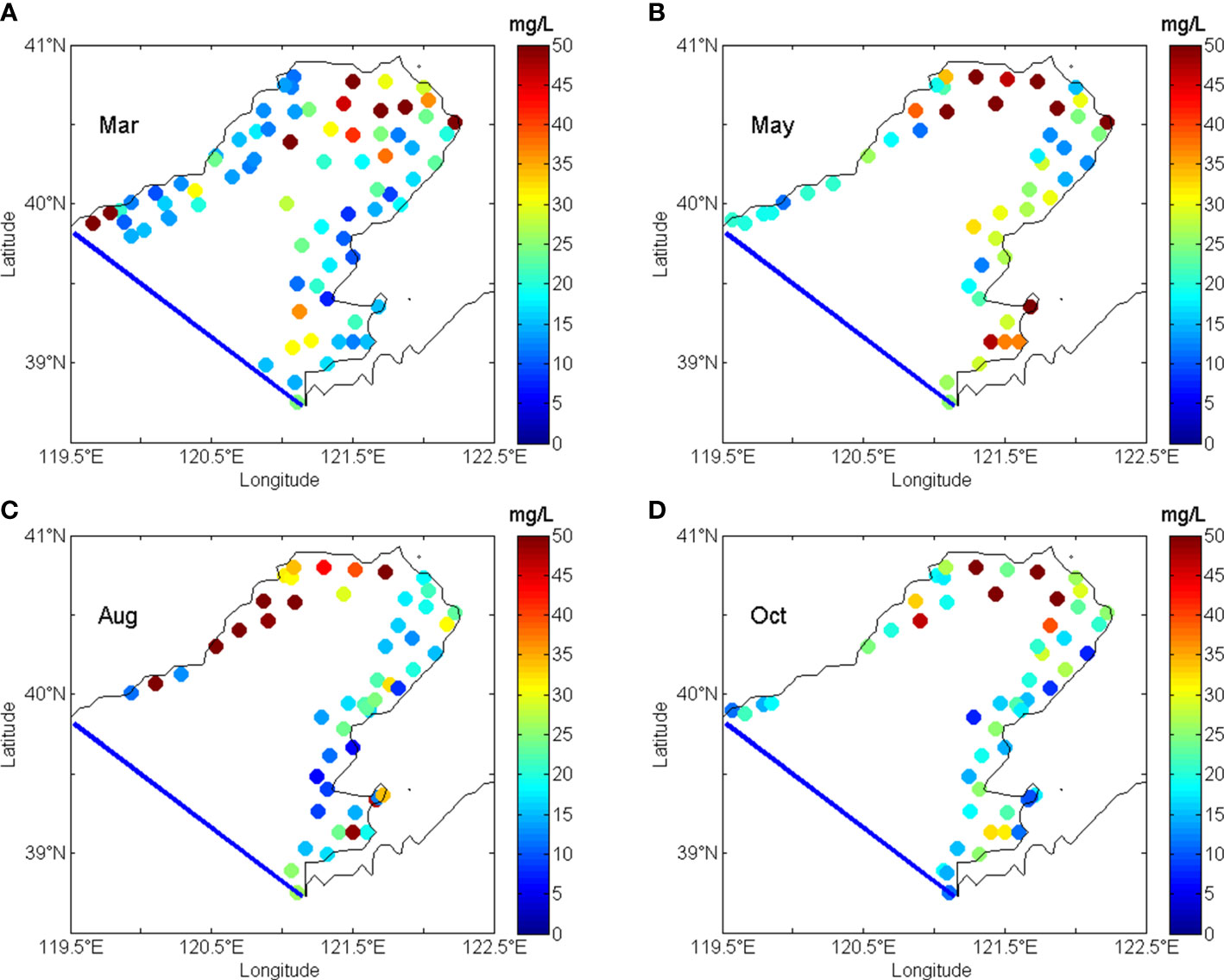
Figure 2 Distributions of observations in the Liaodong Bay. (A–D) show the observations in March, May, August and October, respectively. The blue line is the boundary of the Liaodong Bay. The dots exhibit the monitoring stations. The color of the dots indicates SPM concentration.

2.2. Satellite data of SPM

The satellite data of SPM used in this study was obtained from Korean Geostationary Ocean Color Imager (GOCI) satellite and downloaded from Korea Ocean Satellite Center (http://kosc.kiost.ac.kr/gociSearch/list.nm?menuCd=50&lang=en&url=gociSearch). The satellite provided SPM concentrations in March, May, August and October of 2015 in the Liaodong Bay. GOCI satellite provided gridded output eight times a day with a spatial resolution higher than 1 km. Monthly averaged distributions of SPM in the Liaodong Bay can be obtained from GOCI dataset, and were used to verify the results of dynamically constrained interpolation method in this study.

2.3. Hydrodynamic field of the Liaodong Bay

The hydrodynamic fields used in this study were the results of a hydrodynamic model based on the Princeton Ocean Model (POM). The domain of the hydrodynamic model included the Bohai Sea and the Yellow Sea (34.5°-41°N, 117.5°-127.5°E). The horizontal resolution was 10’in both latitude and longitude, and there were 21 sigma levels in the vertical direction. The open boundary was set at 34.5°N. Four main tidal components (M₂, S₂, K₁ and O₁) were implemented along the open boundary. The Ocean Circulation and Climate Advanced Model (OCCAM) was used to provide the distribution of the climatic circulation in each layer at the open boundary. The initial conditions of temperature and salinity were obtained from NODC (Levitus) World Ocean Atlas 2001. The hydrodynamic model was driven by the wind field. The model was run for one year after spin-up, and the three-dimensional results of currents and water temperature were stored every half an hour. Wang et al. (2013) had verified the hydrodynamic field and used it in the simulation of the Bohai Sea. The Liaodong Bay part of the hydrodynamic flow fields was used in this study. The hydrodynamic fields were spatial interpolated to the grid of our model.

2.4. Interpolation methods without dynamical constraint

2.4.1. Kriging interpolation

The observation data of SPM concentrations recorded as a standard format (x_i,y_i,z_i), i =1,2,3, … , N, where N is the number of observation data. (x_i,y_i,)is the rectangular coordinate converted from the longitude and latitude of the observation station, and z_i is the observed SPM concentration. The interpolated SPM concentration z_j at a given point (x_j,y_j) can be expressed as

$\begin{array}{ll}{z}_j={\displaystyle \sum _{i=1}^N{\beta }_i}·z_i& (1)\end{array}$

where β_iis the interpolation coefficient of Kriging interpolation. Based on different variogram model, β_i can be calculated differently. Kriging interpolation was carried out based on linear variogram model in this study.

2.4.2. Radial basis function interpolation

RBF interpolation has been widely used in spatial interpolation of observation data. The preprocessing of observation data is consistent with Kriging interpolation, and the interpolated SPM concentration at a given point (x_j,y_j) can be expressed as

$\begin{array}{ll}{z}_j=c_0+c_{1}x+c_{2}y+{\displaystyle \sum _{i=1}^{i=N}{\lambda }_i·\phi \left(d_{ij}\right)}& (2)\end{array}$

where d_ij is the distance from the given point (x_j,y_j) to observation (x_j,y_j);φ(d_i,j) is the basis function; c₀, c₁, c₂ and λ_i are constant coefficients. The following five RBFs are usually used, 1) Linear, φ(d_ij)=d_ij , 2) Cubic, φ(d_ij)=d_ij³, 3) Thin plate spline, φ(d_ij)=d_ij²ln(d_ij+1) , 4) Gaussian, φ(d_ij)=exp(−0.5·d_ij²/σ²) , 5) Multi-quadrics, $\phi \left(d_{ij}\right)=\sqrt{1+d_2^{ij}/{\sigma }^2}$. RBF interpolation was carried out based on linear RBF in this study.

2.5. Interpolation method with dynamical constraint based on adjoint assimilation method

Adjoint assimilation is an effective method of data assimilation. It combines the Variation Principle with the Optimization Control Theory, and converts the physical problem to the mathematical problem of finding the minimum value (Sasaki, 1970; Lu and Zhang, 2006). It takes the equations, initial conditions and boundary conditions of model as constraint conditions, and minimizes the cost function representing the errors between the observations and the simulations. Adjoint assimilation method includes three parts: forward model, backward adjoint model and optimization scheme. The adjoint model is derived from Lagrange Multiplier Method. The governing equation of the time-dependent marine ecological model is assumed to be

$\begin{array}{ll}\frac{\partial x}{\partial t}=f\left(x,c\right)& (3)\end{array}$

where x is the state variable of the ecological model; c is the control variable; f represents the nonlinear vector operator; t is the time variable. Lagrange function is defined as

$\begin{array}{ll}L\left(x,c,\lambda \right)=J\left(x,c\right)+\langle \lambda ·G\left(x,c\right)\rangle & (4)\end{array}$

where $G\left(x,c\right)=\frac{\partial x}{\partial t}-f\left(x,c\right)$; J(x,c) is cost function;<-> is the inner product defined on a Hilbert space.

Assuming that there are observations of the state variable x on Ω×T, where Ω means special scale and T means temporal scale, the cost function can be expressed as

$\begin{array}{ll}J\left(x,c\right)=\frac{1}{2}{\displaystyle \underset{\Omega \times T}{\int }{\left(x-x_{obs}\right)}^{2}dwdt}& (5)\end{array}$

Therefore, the constrained minimum problem is transformed into an unconstrained problem about x^*, c^* and λ^* . Consequently, determining the stagnation point of cost function J(x,c) under the restriction of strong constraint condition G(x,c)=0 is equivalent to determining the stagnation point of Lagrange function with respect to state variable x, control variable c and Lagrange multiplier λ . The equations representing stagnation point of Lagrange function are also called Euler-Lagrange equations of constrained minimum value problem. Euler-Lagrange optimal conditions (optimal x^*, c^* and λ^* ) can be determined by the following equations

$\begin{array}{ll}\frac{\partial L}{\partial x}\left(x^{*},c^{*},{\lambda }^{*}\right)=0& (6)\end{array}$

$\begin{array}{ll}\frac{\partial L}{\partial c}\left(x^{*},c^{*},{\lambda }^{*}\right)=0& (7)\end{array}$

$\begin{array}{ll}\frac{\partial L}{\partial \lambda }\left(x^{*},c^{*},{\lambda }^{*}\right)=0& (8)\end{array}$

Equation (7) corresponds to the original model equation. Equation (6), the adjoint equation of equation (7), is a set of equations about Lagrange multiplier. Equation (8) is the gradient expression of cost function J with respect to control variable c. Based on equation (6) and Equation (7), the gradient in equation (8) can be calculated. Since cost function declines in the inverse direction of its gradient with respect to control variable, the direction to optimize the control variable can be determined.

Considering the convection and diffusion processes of SPM and the hydrodynamic conditions of the Liaodong Bay, the material transport model in the Liaodong Bay was built at first and the governing equation was

$\begin{array}{ll}\frac{\partial c}{\partial t}+u\frac{\partial c}{\partial x}+v\frac{\partial c}{\partial y}+w\frac{\partial c}{\partial z}=\frac{\partial }{\partial x}\left(A_H\frac{\partial c}{\partial x}\right)+\frac{\partial }{\partial y}\left(A_H\frac{\partial c}{\partial y}\right)+\frac{\partial }{\partial z}\left(K_H\frac{\partial c}{\partial z}\right)-rc& (9)\end{array}$

where A_H was horizontal diffusion coefficient and K_H was vertical diffusion coefficient; c meant SPM concentration; u, v and w were the flow velocity in the x, y and z directions, respectively; r was degradation rate of SPM and r=0 considering SPM as conserved substance in the Liaodong Bay.

The adjoint equation of Equation (9) was

$\begin{array}{ll}\begin{array}{l}-\frac{\partial c^{*}}{\partial t}-\frac{\partial }{\partial z}\left(K_H\frac{\partial c^{*}}{\partial z}\right)\\ =\frac{\partial u{c}^{*}}{\partial x}+\frac{\partial v{c}^{*}}{\partial y}+\frac{\partial w{c}^{*}}{\partial z}+\frac{\partial }{\partial x}\left(A_H\frac{\partial c^{*}}{\partial x}\right)+\frac{\partial }{\partial y}\left(A_H\frac{\partial c^{*}}{\partial y}\right)-K_c\left(c-\overline{c}\right)\end{array}& (10)\end{array}$

where c^* was adjoint variable of SPM concentration c.

The gradient of the cost function with respect to the SPM concentrations at the initial moment was

$\begin{array}{ll}\begin{array}{l}\frac{\partial J}{\partial c^1}={\left(\frac{\partial c^{*}}{\partial t}\right)}^1+{\left(\frac{\partial u{c}^{*}}{\partial x}\right)}^1+{\left(\frac{\partial v{c}^{*}}{\partial y}\right)}^1+{\left(\frac{\partial w{c}^{*}}{\partial z}\right)}^1\\ \begin{array}{cc}& \end{array}+\frac{\partial }{\partial x}{\left(A_H\frac{\partial c^{*}}{\partial x}\right)}^1+\frac{\partial }{\partial y}{\left(A_H\frac{\partial c^{*}}{\partial y}\right)}^1+\frac{\partial }{\partial z}{\left(K_H\frac{\partial c^{*}}{\partial z}\right)}^1\end{array}& (11)\end{array}$

where superscript 1 denoted the first interation step in the calculation process.

The differential formats of Equations (9) and (10) were expressed as

$\begin{array}{ll}\begin{array}{l}\frac{c_{i,j,k}^{l+1}-c_{i,j,k}^l}{\Delta t}-\left[\frac{K_H\left(c_{i,j,k+1}^{l+1}-c_{i,j,k}^{l+1}\right)}{\Delta z_{k+1/2}·\Delta z_{k+1}}-\frac{K_H\left(c_{i,j,k}^{l+1}-c_{i,j,k-1}^{l+1}\right)}{\Delta z_{k+1/2}·\Delta z_k}\right]=\\ -\frac{u_{i,j,k}^l\left(c_{i+1,j,k}^l-c_{i-1,j,k}^l\right)}{2\Delta x_j}-\frac{v_{i,j,k}^l\left(c_{i,j+1,k}^l-c_{i,j-1,k}^l\right)}{2\Delta y}-\frac{w_{i,j,k}^l\left(c_{i,j,k+1}^l-c_{i,j,k-1}^l\right)}{2\Delta z_k}\\ +\left[\frac{A_H\left(c_{i+1,j,k}^l-c_{i,j,k}^l\right)}{\Delta x_{j+1/2}·\Delta x_{j+1}}-\frac{A_H\left(c_{i,j,k}^l-c_{i-1,j,k}^l\right)}{\Delta x_{j+1/2}·\Delta x_j}\right]\\ +\left[\frac{A_H\left(c_{i,j+1,k}^l-c_{i,j,k}^l\right)}{{\left(\Delta y\right)}^2}-\frac{A_H\left(c_{i,j,k}^l-c_{i,j-1,k}^l\right)}{{\left(\Delta y\right)}^2}\right]\end{array}& (12)\end{array}$

$\begin{array}{ll}\begin{array}{l}\frac{c_{i,j,k}^{*l-1}-c_{i,j,k}^{*l}}{\Delta t}-\left[\frac{K_H\left(c_{i,j,k+1}^{*l-1}-c_{i,j,k}^{*l-1}\right)}{\Delta z_{k+1/2}·\Delta z_{k+1}}-\frac{K_H\left(c_{i,j,k}^{*l-1}-c_{i,j,k-1}^{*l-1}\right)}{\Delta z_{k+1/2}·\Delta z_k}\right]\\ =\frac{\left(u_{i+1,j,k}^l{c}_{i+1,j,k}^{*l}-u_{i-1,j,k}^l{c}_{i-1,j,k}^{*l}\right)}{2\Delta x_j}+\frac{\left(v_{i,j+1,k}^l{c}_{i,j+1,k}^{*l}-v_{i,j-1,k}^l{c}_{i,j-1,k}^{*l}\right)}{2\Delta y}\\ +\frac{\left(w_{i,j,k+1}^l{c}_{i,j,k+1}^{*l}-w_{i,j,k-1}^l{c}_{i,j,k-1}^{*l}\right)}{2\Delta z_k}\\ +\left[\frac{A_H\left(c_{i+1,j,k}^{*l}-c_{i,j,k}^{*l}\right)}{\Delta x_{j+1/2}·\Delta x_{j+1}}-\frac{A_H\left(c_{i,j,k}^{*l}-c_{i-1,j,k}^{*l}\right)}{\Delta x_{j+1/2}·\Delta x_j}\right]\\ +\left[\frac{A_H\left(c_{i,j+1,k}^{*l}-c_{i,j,k}^{*l}\right)}{{\left(\Delta y\right)}^2}-\frac{A_H\left(c_{i,j,k}^{*l}-c_{i,j-1,k}^{*l}\right)}{{\left(\Delta y\right)}^2}\right]-K_c\left(c_{i,j,k}^l-\overline{c_{i,j,k}^l}\right)\end{array}& (13)\end{array}$

The computational domain was 38.5°N-41°N, 119.5°E-122.5°E (the Liaodong Bay) with a 4′ × 4′ horizontal resolution. There were 6 layers in vertical profiles. The depth of each layer from top to bottom was 10m, 20m, 30m, 50m, 75m, and 100m, respectively. The computing time was 30 days and the time step was set to be 6 h. The hydrodynamic field was provided by POM, as described above. In order to improve the simulation accuracy of the adjoint assimilation model, the independent grids were selected every 4 common grids. Only the SPM concentrations of these independent grids needed to be optimized while those of other grid can be calculated by Cressman interpolation. The influencing radius of Cressman interpolation was 1.2 times of the distance between adjacent independent grids. Assimilation stopped when the preset ending condition was satisfied, and the monthly averaged distribution of the model results was taken as the result of interpolation with dynamical constraint.

2.5.1. Reversion of given distribution in ideal experiments

In order to verify the accuracy of the interpolation method with dynamical constraint, two ideal experiments were carried out. An initial distribution was given in the Liaodong Bay. Then the forward model was run for 30 days to obtain distributions at every time step. Idealized observations were picked up from the model-generated concentrations according to the following principle: the sampling locations were the same as the locations of monitoring stations. The adjoint assimilation model was used to optimize the distribution, and the monthly averaged result of the adjoint assimilation model was taken as the result of the interpolation with dynamical constraint. Compared with the given distribution, Mean Absolute Error (MAE) and Normalized Mean Error (NME) can be calculated. The accuracy of the dynamically constrained interpolation method was evaluated by the decrease of the simplified cost function, MAE and NME.

Two ideal experiments were carried out respectively:

1) Assume that the initial distribution of concentrations showed a parabolic surface with downward convex, and the concentration at any grid can be calculated by formula (14). The vertex of the parabolic surface was located at the geometric center of the Liaodong Bay (39.97°N, 121.02°E). The curvature and the maximum value of the parabolic surface were adjusted to make sure the minimum value of the parabolic surface was 10.0 mg/L, which was the SPM background value of the Liaodong Bay and the average value of the parabolic surface was 32.3 mg/L, which was the average value of the observational SPM concentrations.

2) Assume that the initial distribution of concentrations increased uniformly with the distance from the mouth of the Liaodong Bay, and the concentration at any grid can be calculated by formula (15).The minimum value of the given distribution of concentrations was 10.0 mg/L, which was the SPM background value of the Liaodong Bay. The constant values were adjusted to make sure that the gradient of the given concentration was perpendicular to the boundary line between the Liaodong Bay and the central Bohai Sea. The value of the gradient was adjusted to make sure the average value of the given distribution was 32.3 mg/L, which was the average value of the observational SPM concentrations.

$\begin{array}{ll}-25\times \left[{\left(lon\left(i\right)-121.02\right)}^2+{\left(lat\left(j\right)-39.97\right)}^2\right]+ 45.3& (14)\end{array}$

$\begin{array}{ll}18\times \frac{\left|-0.6743\times lon\left(i\right)-lat\left(j\right)+120.4112\right|}{\sqrt{{\left(-0.6743\right)}^2+1}}+10.0& (15)\end{array}$

where lon(i) indicated the longitude and lat(j) indicated the latitude. The index triplet (i, j) was a pointer to certain grid in the given initial field. We guessed that the initial concentration of the model at any grid was 10.0 mg/L and adjusted the distributions using adjoint assimilation model.

2.5.2. Dynamically constrained interpolation in practical applications

The concentrations of SPM in the Liaodong Bay in March, May, August and October 2015 were interpolated with dynamical constraint. The initial concentration at any grid was set as the average value of the observations. With the simulation of adjoint assimilation model for 30 days, the distributions of the SPM concentrations can be obtained, meanwhile MAEs and NMEs at the grid of observation stations can be calculated.

2.6. Cross-validation

Cross-validation is an effective method to evaluate the results of interpolations (Robinson and Metternicht, 2006; Hofierka et al., 2007; Wise, 2011; Etherington, 2020). The leave-one-out cross-validation method was adopted in this study. All observations were randomly and averagely divided into N groups. The N-1 groups were used in spatial interpolation to obtain the SPM concentration at any grid. Since the remaining 1 group had not been used in interpolation, it can be used as test data to check the interpolated distribution. MAEs and NMEs were calculated by combining the interpolated distribution with test data. Their calculation formulas were

$\begin{array}{ll}MAE=\frac{1}{M}{\displaystyle \sum _{i=1}^M\left|O_{\mathrm{int}erp}-O_{obs}\right|}& (16)\end{array}$

$\begin{array}{ll}NME=\frac{1}{M}{\displaystyle \sum _{i=1}^M\frac{\left|O_{\mathrm{int}erp}-O_{obs}\right|}{O_{obs}}}& (17)\end{array}$

where O_obs was SPM observation in the test data; O_interp was interpolated SPM concentration, and the location of O_interp was the same as the location of O_obs; M was the quantity of test data. The experiment was repeated N times, hence each group of observations was used as test data by turns. The averaged MAE and NME of the N times were calculated as the indexes to evaluate interpolation methods. A 10-fold cross-validation method was adopted in this study (N=10).

3. Result

3.1. Application of the interpolation method with dynamical constraint in two ideal experiments

Two ideal experiments were carried out to testify the feasibility and validity of the interpolation methodology with dynamical constraint. The initial distribution, the idealized observations and the evaluation indexes in the ideal experiment were described in Section 2.5.1.

3.1.1. Ideal experiment I: Distribution of concentrations shows a parabolic surface

In Ideal Experiment I, the given initial distribution of SPM concentrations in the Liaodong Bay showed a parabolic surface with downward convex. SPM concentrations had the maximum value of 45.3 mg/L in the central Liaodong Bay and decreased outward. The low values appeared around the coastal areas, and the minimum value of 10.0 mg/L occurred in the top and the mouth of the bay. The concentration of SPM at any grid can be calculated by formula (14). The interpolation method with dynamical constraint was used to calculate the interpolated distribution. The given initial and the interpolated distributions of SPM concentrations were compared in Figure 3. It was obvious that the distribution of the dynamically constrained interpolation was consistent with the given initial distribution, which had the maximum concentration in the central Liaodong Bay and decreased in all direction. The interpolated distribution of SPM concentrations also showed a parabolic surface with downward convex analogously.

FIGURE 3

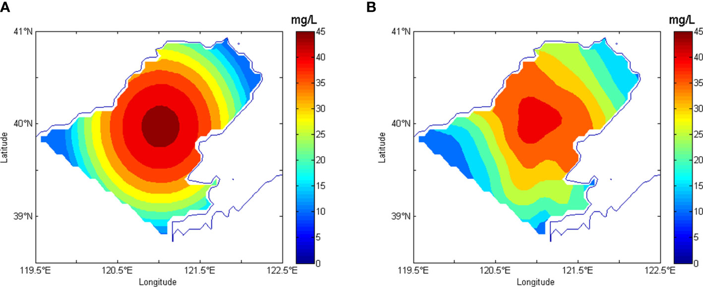
Figure 3 Interpolated results of given initial distribution of SPM that shows a parabolic surface with downward convex. (A) is the given distribution in Ideal Experiment I. (B) is interpolated distribution derived from dynamically constrained interpolation. The observations using in the interpolation were picked up from the model-generated concentrations based on given distributions.

To quantitatively compare the interpolated and observed concentrations, MAE and NME were calculated by formula (16) and formula (17). The initial values of MAE and NME and the final values of MAE and NME after 100 calculating steps of the adjoint assimilation were compared in Table 1. The final values of MAE and NME were 1.003 mg/L and 0.043, and decreased by 94.6% and 92.9%, respectively. The final NME was 0.043, which indicated that the final errors of the interpolated results accounted for only 4.3% of the observations. The reduction ratio of the simplified cost function was also shown in Table 1. The cost function decreased by 99.8%. These high reduction ratios suggested that dynamically constrained interpolation based on the adjoint assimilation model greatly reduced the differences between the interpolated distribution and the observed distribution during the interpolation process. An accurate distribution of SPM concentrations was obtained using the interpolation method with dynamical constraint.

TABLE 1

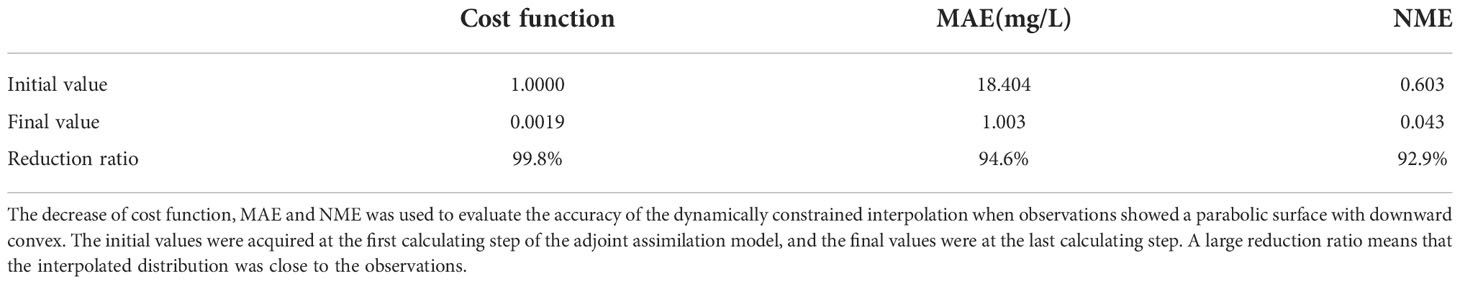
Table 1 The cost function, MAE and NME of Ideal Experiment I.

3.1.2. Ideal experiment II: Distribution of concentrations increases uniformly

In Ideal Experiment II, the given initial distribution exhibited a uniform increase of SPM concentrations from the mouth to the top of the bay. SPM concentrations had the lowest value of 10.0 mg/L along the mouth and the highest value of 45.6 mg/L around the top of the Liaodong Bay. The concentration of SPM at any grid can be calculated by formula (15).The interpolation method with dynamical constraint was used to obtain the interpolated distribution. The given initial distribution and the interpolated distribution of SPM concentrations were compared in Figure 4. It suggested that the distribution of the dynamically constrained interpolation exhibited high agreement with the given initial distribution. SPM concentrations had the minimum value along the mouth of the Liaodong Bay and then increased gradually to the maximum value near the top.

FIGURE 4

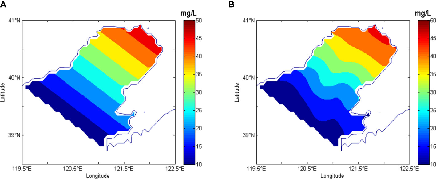
Figure 4 Interpolated results of given initial distribution of SPM that increases uniformly with the distance from the mouth. (A) is the given initial distribution in Ideal Experiment II. (B) is interpolated distribution derived from dynamically constrained interpolation. The observations using in the interpolation were picked up from the model-generated concentrations based on given distributions.

The simplified cost function decreased by 99.9% (Table 2). The final values of MAE and NME were 0.924 mg/L and 0.036, which decreased by 95.1% and 93.8% respectively. The final NME was 0.036, which indicated that the final errors of the interpolated results accounted for only 3.6% of the observations. It was obvious that the dynamically constrained interpolation based on the adjoint assimilation model greatly reduced the differences between the interpolated and the observed distributions. An accurate distribution of SPM concentrations can be obtained using interpolation method with dynamical constraint in Ideal Experiment II.

TABLE 2

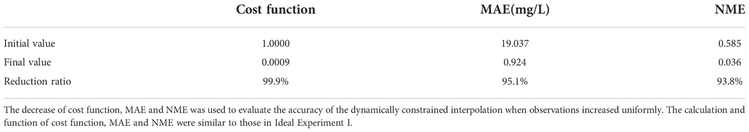
Table 2 The cost function, MAE and NME of Ideal Experiment II.

Furthermore, the results of the two ideal experiments were compared with the similar ideal experiments carried out in previous studies. Wang et al. (2013) set four ideal experiments respectively in the Bohai Sea. The given distributions showed a parabolic surface with upward convex, a parabolic surface with downward convex, a conical surface with upward convex and a conical surface with downward convex in four ideal experiments respectively. The cost function decreased by 96.3%, 91.7%, 95.6% and 90.9%, respectively. The MAE decreased by 88.7%, 86.9%, 92.5% and 92.1%, respectively. The NME decreased by 85.2%, 87.4%, 86.5% and 87.1%, respectively. Huang et al. (2021) set a similar ideal experiment in the Laizhou Bay. The concentrations of petroleum hydrocarbon pollutants decreased exponentially in the given distribution of ideal experiment. The MAE decreased by 88.40%. Their models exhibited high accuracy during simulation. In this study, the reduction ratios of the cost functions, MAE and NME were larger, which proved that the errors were smaller.

3.2. Application of the interpolation method with dynamical constraint in practical experiments

SPM observations in March, May, August and October 2015 were used for dynamically constrained interpolation. Most of the observation stations were located in the coastal area, while the observation stations in the central Liaodong Bay were rare (Figure 2). In March of 2015 (Figure 2A), a high value area of the observations appeared near the top of the Liaodong Bay. There were two high value regions of observations on the northwest and the southeast side of the mouth. The maximum value of 101.8 mg/L occurred at the top of the Liaodong Bay. The SPM observations along the northwest and southeast coastal area were low. In May (Figure 2B), the SPM observations around the top of the bay were still high. Another high value area of observations was in the semi-enclosed bay near the Dalian city. The maximum value of the observations was 547.0 mg/L, which was observed near the top. In August (Figure 2C), the SPM observations on the northwest side of the Liaodong Bay were much higher than those on the southeast side. The observations near the Dalian city were still high. The maximum value of 124.0 mg/L occurred on the northwest side of the Liaodong Bay. In October (Figure 2D), there was still a high value region of observations in the top area. The maximum value was observed here, which was 464.0 mg/L. The observations near the Dalian city were also high.

Based on the SPM observations of four months, the distributions of SPM were derived from dynamically constrained interpolation, which were shown in Figure 5. The general trend of the distributions was that the concentration was high in the top and north of the Liaodong Bay, and low in the southeast of the Liaodong Bay, which was basically consistent with the distributions of observations (Figure 2). In March of 2015 (Figure 5A), an area of high SPM concentrations appeared in the northeast part of the bay, with the values higher than 40 mg/L. A band of high values extended from northeast to southwest along the central bay, and then turned to the east area of the mouth of the bay. Another area with high values appeared in the west end of the mouth. Along the southeast and northwest coastline of the bay, there were areas with low concentrations, with values lower than 15 mg/L. In May (Figure 5B), the high SPM concentrations area in the northeast part of the bay was enlarged, and the gradient of SPM concentrations was also increased. The concentration of the area was higher than 50 mg/L. A band of high concentrations extending from the central bay to the central area of bay mouth occurred. The SPM concentrations in the semi-enclosed bay near the Dalian city were higher than 30 mg/L, forming a high value area. The low concentration areas along the southeast and northwest coastline were still there, while the concentration increased. In August (Figure 5C), the high-values band across the central Liaodong Bay, appearing in March and May, translated to the northwest coastline. From the top to the mouth of the bay, the concentrations of the three high value areas on the band were greater than 50.0 mg/L, 50.0 mg/L and 30.0 mg/L, respectively. The high value areas near the Dalian city still appeared, with the maximum values higher than 35.0 mg/L. The SPM concentrations of the southeast part of the Liaodong Bay were lower than those of the northwest part of the bay. There were two low value areas occurred here, with concentrations lower than 15 mg/L and 10 mg/L respectively. In October (Figure 5D), the SPM concentrations in the northeast part of the bay were higher than 50 mg/L, forming a high value area with high value of gradient of SPM concentrations. The other high value area was found in the northwest area of the mouth, with SPM concentrations higher than 25 mg/L. The semi-enclosed bay in the southeast of the mouth of the Liaodong Bay remained a high value area, with SPM concentrations higher than 20 mg/L. A band of low values extended along the southeast coastline, with concentrations lower than 15 mg/L.

FIGURE 5

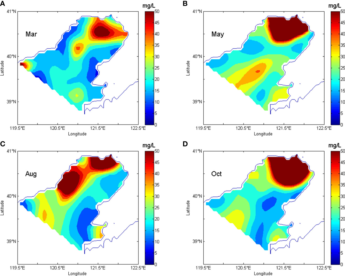
Figure 5 Interpolated distributions with dynamical constraint of SPM concentrations in the Liaodong Bay. (A) is the distribution obtained by dynamically constrained interpolation based on SPM observations in March 2015. (B–D) are the interpolated distributions of May, August and October 2015, respectively.

3.3. Application of Kriging interpolation and RBF interpolation in practical experiments

The interpolated distribution of SPM concentrations in the Liaodong Bay had been obtained by interpolation method with dynamical constraint in Section 3.2. The interpolation method without dynamical constraint such as Kriging interpolation and RBF interpolation were also widely used in marine research. In this part, to verify the superiority of interpolation method with dynamical constraint over interpolation method without dynamical constraint, the spatial interpolation of SPM concentrations using Kriging method and RBF method was carried out respectively. Kriging interpolation and RBF interpolation were used to interpolate SPM concentration data observed in the Liaodong Bay in 2015. The interpolated distributions of SPM concentrations using Kriging interpolation and RBF interpolation were shown in Figures 6, 7 respectively.

FIGURE 6

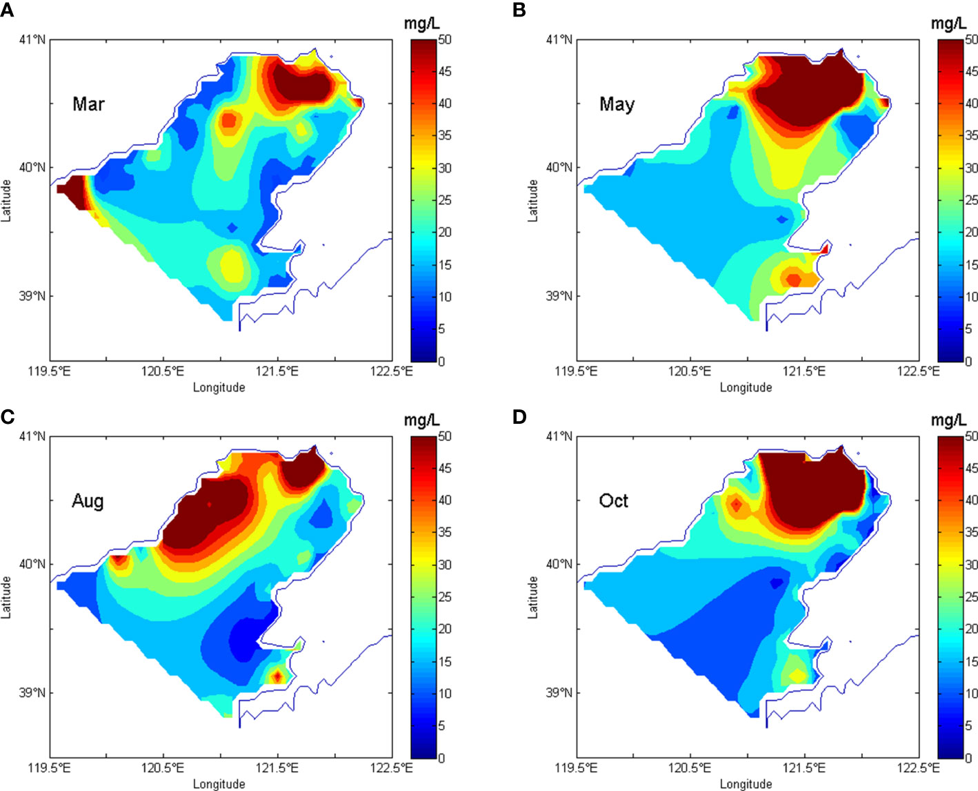
Figure 6 Interpolated distributions of SPM concentrations in the Liaodong Bay using Kriging interpolation. (A) is the distribution obtained by Kriging interpolation based on SPM observations in March 2015. (B–D) are the interpolated distributions of May, August and October 2015, respectively.

FIGURE 7

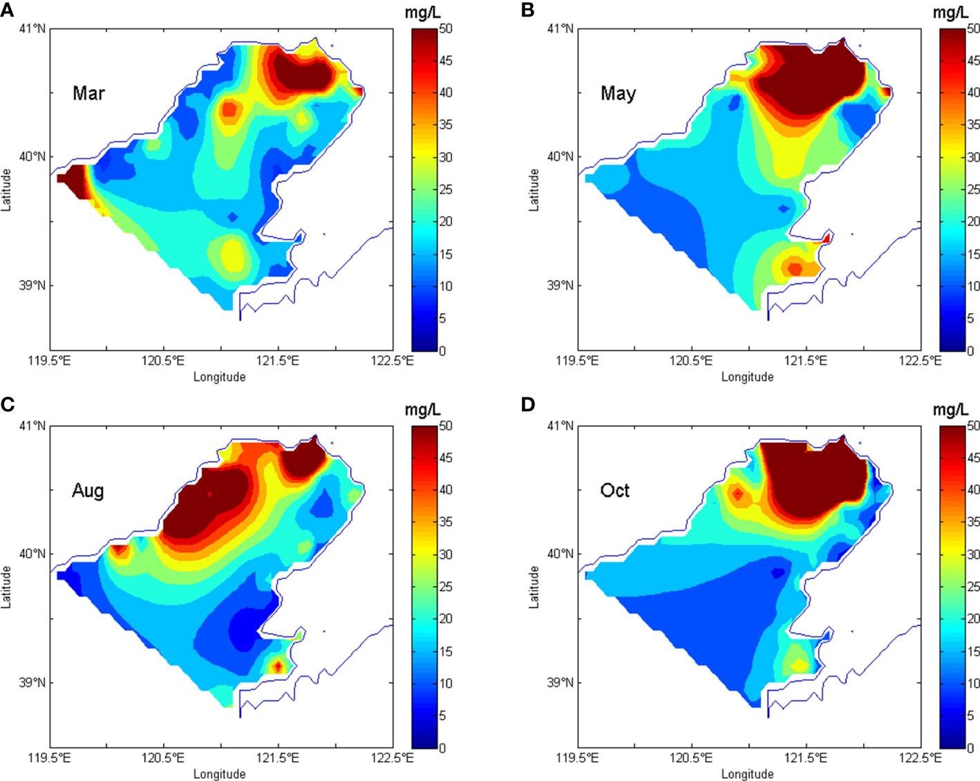
Figure 7 Interpolated distributions of SPM concentrations in the Liaodong Bay using RBF interpolation. (A) is the distribution obtained by RBF interpolation based on SPM observations in March 2015. (B–D) are the interpolated distributions of May, August and October 2015, respectively.

The interpolated distributions of Kriging interpolation, RBF interpolation and dynamically constrained interpolation were roughly similar. The high value and low value areas appearing in the interpolated results of the three interpolation methods were generally consistent with the observed distributions of SPM concentrations (Figure 2). As shown in Figures 5A, 6A, 7A, a banded high value region of SPM concentrations appeared in the central area of the Liaodong Bay. The high value area of SPM concentrations occurred in the top area of the bay, with the concentrations greater than 50 mg/L. The low values of SPM concentrations lower than 5 mg/L were in the coastal area at the northwest and southeast of Liaodong Bay. Figures 5C, 6C, 7C indicated that the interpolated results of the three interpolation methods all had a high value area of SPM concentrations in the top of the Liaodong Bay, with the concentrations greater than 50 mg/L. The low value of SPM concentrations lower than 15 mg/L appeared in the southeast of the Liaodong Bay. The interpolated distributions of the three interpolation methods all had a high value around the top of the Liaodong Bay in March and October, with the concentrations of SPM greater than 50 mg/L (Figures 5B, D, 6B, D, 7B, D).

Some high value regions in the interpolated distributions of dynamically constrained interpolation didn’t appear in the interpolated distributions of Kriging interpolation and RBF interpolation, such as the high value region in the northwest area of the mouth of the Liaodong Bay in October. The accuracy and the authenticity of interpolation with dynamical constraint should be tested.

4 Discussion

4.1. Cross validations of the interpolation methods

The 10-fold cross-validation was used to evaluate and compare the results of unconstrained and dynamically constrained interpolation methods, and the averaged MAEs of each method were considered to be the evaluation index (Table 3). Beside Kriging and RBF interpolation, five more unconstrained interpolation methods were also carried out in this section to further test the accuracy of different unconstrained interpolation methods. They were the Cressman interpolation with the influencing radius of 0.40°, the Cressman interpolation with influencing radius of 0.75°, the minimum curvature interpolation, the nearest neighbor value interpolation and the inverse-distance weighting interpolation.

TABLE 3

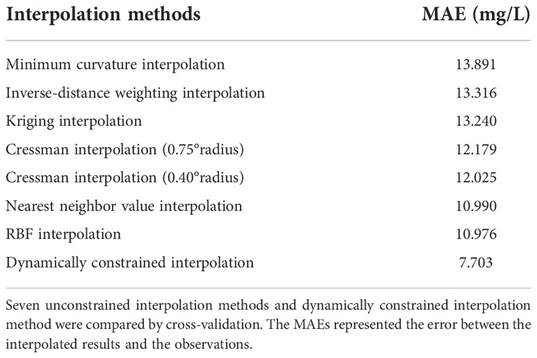
Table 3 Cross-validation results of eight interpolation methods.

Since the rand-size relationship of MAEs of these interpolation methods in the four months were the same, the results of August were described as below. Among the seven unconstrained interpolation methods, the averaged MAE of RBF interpolation was the minimum, which was 10.976 mg/L. The averaged MAE of the minimum curvature interpolation was the maximum, followed by the inverse-distance weighting interpolation. The averaged MAEs of the nearest neighbor value interpolation, the Cressman interpolation with influencing radius of 0.40° and the Cressman interpolation with influencing radius of 0.75° was 10.990, 12.025 and 12.179 mg/L, which were lower than the averaged MAE of Kriging interpolation which was 13.240 mg/L. It was indicated that the Cressman and nearest neighbor value interpolations were more accurate than the Kriging interpolation. However, the distributions of these three interpolation methods weren’t reasonable. The interpolated distribution of SPM concentrations of Cressman interpolation with influencing radius of 0.40° was incompletely interpolated since the influencing radius of 0.40° was not large enough to guarantee the results at every grid can be calculate by the observations. The interpolated distribution of Cressman interpolation with influencing radius of 0.75° was excessively smooth because the influencing radius was too large and too many observations were taken into calculation. The distribution derived from the nearest neighbor value interpolation was also incompletely interpolated and the concentration gradients at some grids were infinite. Kriging interpolation was more accurate than these three interpolation methods because the interpolated distribution of SPM concentrations was more reasonable. RBF interpolation was the most accurate among the unconstrained interpolation methods, followed by Kriging interpolation. Among the seven unconstrained interpolation methods, RBF and Kriging behaved much better.

When using the interpolation method with dynamically constraint, the averaged MAE and NME of all observation stations were 7.703 mg/L and 0.277 respectively. The averaged MAE of dynamically constrained interpolation method was 29.8%-44.5% lower than that of the seven unconstrained interpolation methods. The averaged MAE and NME of Kriging interpolation were 13.240 mg/L and 0.349 respectively, and those of RBF interpolation were 10.976 mg/L and 0.304 respectively. It was suggested that the averaged MAE of the dynamically constrained interpolation method was 41.8% and 29.8% smaller than those of Kringing and RBF, while the averaged NME was 20.6% and 8.8% smaller respectively.

The results of cross-validations indicated a better agreement between the distribution from the dynamically constrained interpolation and observations. However, the cross-validation only considered the errors between the interpolation results and the observations at the monitoring stations. In the areas where there was lack of observations, whether the interpolated distributions were reasonable and true should be further tested using more observations.

4.2. Influences of hydrodynamic processes on the interpolation of SPM concentrations

In Section 4.1, it was proved that RBF and Kriging interpolations were the two most accurate methods among the seven unconstrained interpolation methods, and the dynamically constrained interpolation was more accurate than RBF and Kriging interpolation. However, whether the interpolated distributions were consistent with the observations was more important. In this section, the influences of the currents (Figure 8) on the interpolated distributions were discussed, and the distributions of dynamically constrained and unconstrained interpolations were compared with the satellite-derived distributions obtained from GOCI (Figure 9). The satellite-derived SPM concentrations (Figure 9) were smaller than the in-situ observations (Figure 2) and the interpolated concentrations (Figures 5–7) based on the in-situ observations. The satellite data is frequently missing, because of the cloud cover, the variation of irradiances and the effect of sensor spatial resolution. Therefore, compared with the in-situ observations, the satellite-derived concentrations will underestimate the SPM concentration (Wielicki and Parker, 1992; Eleveld et al., 2014; Jia et al., 2021 and Mei et al., 2014). However, the underestimation will not affect the trend of satellite-derived SPM distributions and the satellite-derived distributions can be used to verify the interpolated distributions (Xu et al., 2020). Since the distributions of Kriging interpolation was similar to those of RBF interpolation and the results of cross-validation proved that RBF interpolation was more accurate, only the distributions of RBF interpolation was used to be compared with the distributions of dynamically constrained interpolation in this section.

FIGURE 8

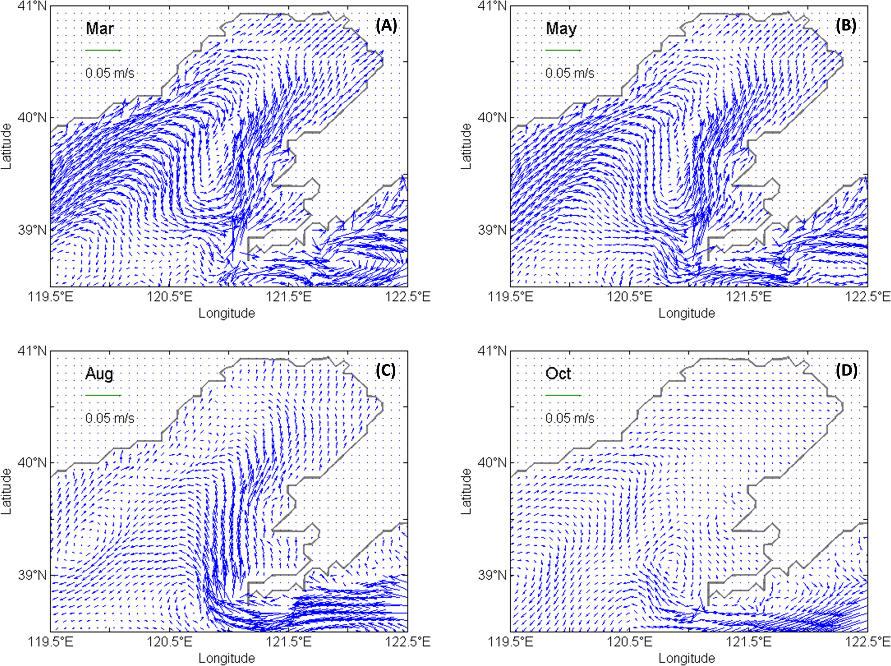
Figure 8 Monthly averaged currents field in the Liaodong Bay. The hydrodynamic fields were calculated by POM and had been validated by Wang et al. (2013). The Liaodong Bay part of the hydrodynamic field was interpolated to the grid of our model. (A–D) show the monthly averaged currents fields in March, May, August and October 2015, respectively.

FIGURE 9

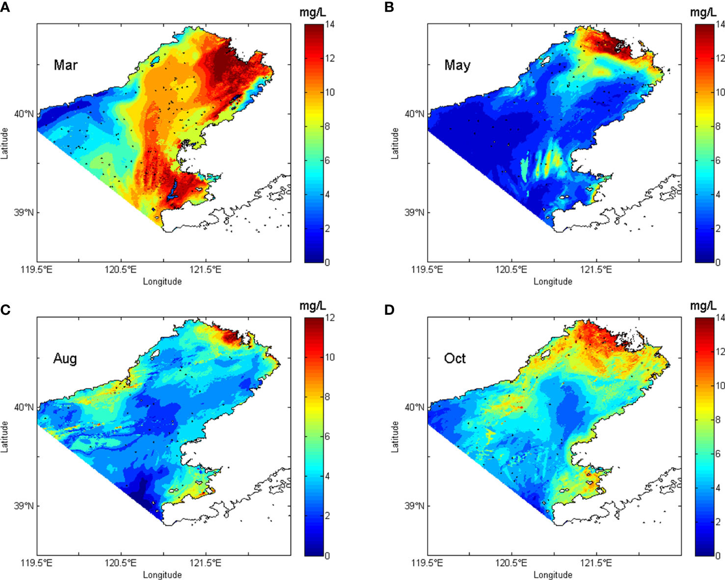
Figure 9 Monthly averaged SPM concentrations in the Liaodong Bay obtained from satellite. Satellite observations were obtained from GOCI. (A) shows the derived monthly averaged distribution of SPM concentrations in March 2015. (B–D) are the distributions of May, August and October 2015, respectively.

In March of 2015, the distribution derived from dynamically constrained interpolation (Figure 5A) was similar to the GOCI-derived distribution (Figure 9A). Water flowed into the Liaodong Bay along the northwest and the southeast coastline, and flowed out of the Liaodong Bay through the central area (Figure 8A). Water with low SPM concentration was transported along the coastline from the central Bohai Sea to the top of the Liaodong Bay. Meanwhile, water with high SPM concentration was transported through the central Liaodong Bay from the top to the mouth of the Liaodong Bay. Consequently, in the distributions from dynamically constrained interpolation and satellite, the low values of SPM concentration appeared in the coastal areas of the Liaodong Bay and a band of high concentration extended from the top through the center to the mouth of the bay. Although the influences of currents weren’t considered in the RBF interpolation process, the distribution from RBF interpolation (Figure 7A) was also consistent with the satellite-derived distribution, because the quantity of observations was large and the observation stations covered a large enough area in March.

In May, the currents were similar to those in March (Figure 8B). The currents brought the water with low SPM concentration into the bay from the central Bohai Sea to the top of the bay along the coastline, and brought the water with high SPM concentration out of the bay from the top to the mouth through the center of the bay. In the distribution of the dynamically constrained interpolation (Figure 5B), a high value area appeared around the top of the bay. The other high value area occurred in the central area of the mouth of the Liaodong Bay. In the satellite-derived distribution (Figure 9B), a same high value area appeared at the top of the bay. There was also a high value area in the bay mouth area, but it was closer to the southeast side of the bay than in the distribution of the dynamically constrained interpolation. Although the location of the area in the bay mouth (Figure 5B) was not totally consistent with that derived by satellite data (Figure 9B), the results of dynamically constrained interpolation successfully reproduced the area with high SPM concentrations in the bay mouth. However, the high values of SPM concentration in the central region of the mouth was not captured in the distribution of the RBF interpolation (Figure 7B), because of not considering the influences of hydrodynamic processes and lack of observations.

In August, the inflow at the northwest side of the Liaodong Bay became weak. Water flowed into the Liaodong Bay along the southeast side and out of the Liaodong Bay along the northwest side (Figure 8C). Water with low SPM concentration was transported along the southeast side into the Liaodong Bay and water with high SPM concentration was taken out of the Liaodong Bay along the northwest side. Therefore, the low values of SPM concentration appeared in the southeast Liaodong Bay, while the high values appeared in the northwest. The distribution of the dynamically constrained interpolation (Figure 5C) was similar to the satellite-derived distribution (Figure 9C). The SPM concentrations in the northwest part of the Liaodong Bay were higher than those in the southeast. In the distribution of the dynamically constrained interpolation, a high value area occurred in the northwest of the mouth of the Liaodong Bay (Figure 5C). The same high values of SPM concentration also appeared in the SPM distribution obtained from GOCI satellite (Figure 9C). However, the same high value region didn’t appear in the distribution of RBF interpolation (Figure 7C). There was a lack of observations in this area (Figure 2C). Besides, the influences of currents were not considered in the RBF interpolation. As a result, the high values here were not reflected in the distribution of RBF interpolation.

In October, the currents in the Liaodong Bay (Figure 8D) were similar to those in August but much weaker. Water flowed into the Liaodong Bay along the southeast coastline and out of the bay along the northwest coastline slowly. The SPM concentrations in the northwest of the bay were higher than those in the southeast of the bay. There were two high value areas found in the distribution of the dynamically constrained interpolation (Figure 5D) and GOCI-derived distribution (Figure 9D). The maximum SPM concentration occurred in the region near the top of the bay and the gradient of SPM concentration was obvious. Besides, a high value area was found in the northwest of the mouth of the Liaodong Bay. The high values of SPM concentration near the top was also reflected in the distribution of RBF interpolation (Figure 7D), because the currents here were weak and the observations here were abundant (Figure 2D). However, the high values around the mouth of the Liaodong Bay was not captured by the interpolated distribution using RBF interpolation (Figure 7D), because the influences of currents were not taken into consider and the observations here were rare (Figure 2D).

In this part, we discussed the influence of hydrodynamic processes on the interpolated distribution with dynamical constraint, and verified the interpolated results (Figure 5) with SPM distributions from satellite (Figure 9). Dynamically constrained interpolation can provide the distributions of SPM concentrations more consistent with the observations than the unconstrained interpolation methods. Besides, dynamically constrained interpolation can fully consider the influence of hydrodynamic processes, and provided the interpolated concentration similar to the actual in the area missing observations.

4.3. Factors controlling the temporal and spatial variations of SPM concentrations in the Liaodong Bay

Based on the SPM observations of March, May, August and October 2015 in the Liaodong Bay and interpolated SPM distributions obtained from dynamically constrained interpolation, the influencing factors of temporal and spatial variations of SPM concentrations were discussed in this part. The average value of SPM concentrations observed in March was 23.6 mg/L, the maximum value was 101.8 mg/L, and the minimum value was 7.4 mg/L. The average value of SPM concentrations observed in May was 42.0 mg/L, the maximum value was 547.0 mg/L, and the minimum value was 11.0 mg/L. The average value of SPM concentrations observed in August was 28.0 mg/L, the maximum value was 124.0 mg/L, and the minimum value was 5.6 mg/L. The average value of SPM concentrations observed in October was 39 mg/L, the maximum value was 464 mg/L, and the minimum value was 7.2 mg/L. The results of spatial interpolation with dynamical constraint indicated that the averaged SPM concentration of May was the highest, which was consistent with the observations. The maximum value of SPM concentration of May was located near the estuary area. Besides, the maximum SPM concentration of May was also the highest.

SPM concentrations in the Liaodong Bay were greatly affected by river’s run-off SPM inputs. Based on the River Sediment Bulletin of China published by the Ministry of Water Resources of the People’s Republic of China (http://www.mwr.gov.cn), the river discharge and sediment discharge in the estuary of the Liao River Basin were analyzed. The river discharge in March, May, August and October 2015 was 60, 220, 100 and 70 million m3, respectively. The sediment discharge in March, May, August and October 2015 was 16, 68, 16 and 3 thousand tons, respectively. The concentration of sediment in the water discharged from the estuary of Liao River Basin in March, May, August and October 2015 was 266.7, 309.1, 160.0 and 42.9 mg/L, respectively. The sediment discharge and concentration of sediment were both the highest in May. It is presumed that the increase of the river run-off SPM inputs in May leaded to the increase of the SPM concentration in the Liaodong Bay. This indicates that the SPM discharge of the estuary area may be an important reason for the variations of SPM concentration in the Liaodong Bay.

The currents in the Liaodong Bay also had influences on the distributions of SPM concentrations, which were discussed in Section 4.2. The SPM concentration tended to be high in the area currents flowing from the top of the bay out of the bay. Low concentrations tended to occur in the area currents flowing from the outer bay to the inner bay. There was a permanent northeast flow in the southeast side of Liaodong Bay, bring fresh water from the central Bohai Sea into the Liaodong Bay, which made the SPM concentration in the southeast side of Liaodong Bay low throughout the year. In March and May, the currents flowed from the top of the bay out of the bay through the central Liaodong Bay, and the value of the SPM concentration of the central Liaodong Bay was higher than other areas. In August and October, the currents flowed from the top of the bay out of the bay along the northwest Liaodong Bay, and the high value of SPM concentration occurred there.

5. Conclusion

In this study, an interpolation method with dynamical constraint was established to interpolate the SPM concentrations. The results of dynamically constrained interpolation were optimized iteratively with the adjoint assimilation method. In two ideal experiments, the final NMEs after 100 calculating steps were 0.043 and 0.036, which means the final errors of the interpolated results accounted for only 4.3% and 3.6% of the observations. The results proved the accuracy of dynamically constrained interpolation.

In the cross-validation experiments, the averaged MAE of dynamically constrained interpolation was 7.703 mg/L, which was 29.8%-44.5% lower than that of other unconstrained interpolation methods. Compared with unconstrained interpolation methods, dynamically constrained interpolation provided more consistent interpolated SPM concentrations at the observation stations. In addition, the averaged MAE of RBF interpolation method was 10.976 mg/L, which was the lowest among the seven unconstrained interpolation methods. RBF interpolation method was the best choice among unconstrained interpolation methods when dynamically constrained interpolation cannot be used due to the lack of dynamically constrained conditions.

The interpolated distributions were compared with the distributions obtained from satellite. The GOCI satellite-derived distributions of SPM were similar to the distributions of interpolation method with dynamical constraint. However, because of the lack of observations in some areas of Liaodong Bay and not taking the hydrodynamic processed into consider, there were many high value regions weren’t captured by the RBF interpolation distributions, which existed in the satellite distributions. It was revealed that the hydrodynamic processes had important influence on the distributions of SPM, which could be used to improve the accuracy of interpolations.

The determining factors of the temporal and spatial variations of SPM concentrations in the Liaodong Bay were analyzed. The SPM concentration in the Liaodong Bay was highest in May due to the influence of the change of river SPM discharge in the Liao River Basin. Under the influence of the flow field, the SPM concentration in the northwest and the central Liaodong Bay was higher than that in the southeast Liaodong Bay.

Data availability statement

The original contributions presented in the study are included in the article/supplementary materials. Further inquiries can be directed to the corresponding author.

Author contributions

Conceptualization, JS. Methodology, JS. Software, HG. Validation, JS and XM. Formal analysis, HG and HP. Investigation, XM and HP. Data curation, HP. Writing—original draft preparation, HG. Writing—review and editing, JS and HG. Supervision, XL. Project administration, XL. and XM. All authors contributed to the article and approved the submitted version.

Funding

This paper was supported by the National Natural Science Foundation of China (U1806214 and 42176022).

Acknowledgments

We are grateful to all those who helped us work out our problems during this study. We express our heartfelt gratitude to all the group members for their helpful assistance and advice.

Conflict of interest

The authors declare that the research was conducted in the absence of any commercial or financial relationships that could be construed as a potential conflict of interest.

Publisher’s note

All claims expressed in this article are solely those of the authors and do not necessarily represent those of their affiliated organizations, or those of the publisher, the editors and the reviewers. Any product that may be evaluated in this article, or claim that may be made by its manufacturer, is not guaranteed or endorsed by the publisher.

References

Bourgain P., Gascard J. C. (2011). The Arctic ocean halocline and its interannual variability from 1997 to 2008. Deep Sea Res. Part I: Oceanographic Res. Papers 58 (7), 745–756. doi: 10.1016/j.dsr.2011.05.001

CrossRef Full Text | Google Scholar

Chen H., Cao A., Zhang J., Miao C., Lv X. (2014). Estimation of spatially varying open boundary conditions for a numerical internal tidal model with adjoint method. Mathematics Comput. Simulation 97, 14–38. doi: 10.1016/j.matcom.2013.08.005

CrossRef Full Text | Google Scholar

Cloern J. E. (1987). Turbidity as a control on phytoplankton biomass and productivity in estuaries. Continental shelf Res. 7 (11-12), 1367–1381. doi: 10.1016/0278-4343(87)90042-2

CrossRef Full Text | Google Scholar

Davis P. J. (1975). Interpolation and approximation (New York: Dover Publications (reprint)). doi: 10.1112/jlms/s1-39.1.568

CrossRef Full Text | Google Scholar

Dou Y., Li J., Zhao J., Wei H., Yang S., Bai F., et al. (2014). Clay mineral distributions in surface sediments of the liaodong bay, bohai Sea and surrounding river sediments: Sources and transport patterns. Continental Shelf Res. 73, 72–82. doi: 10.1016/j.csr.2013.11.023

CrossRef Full Text | Google Scholar

D’Sa E. J., Miller R. L., Castillo C. D. (2006). Bio-optical properties and ocean color algorithms for coastal waters influenced by the Mississippi river during a coldfront. Appl. Op. 45, 7410–7428. doi: 10.1364/AO.45.007410

CrossRef Full Text | Google Scholar

Eleveld M. A., van der Wal D., Van Kessel T. (2014). Estuarine suspended particulate matter concentrations from sun-synchronous satellite remote sensing: Tidal and meteorological effects and biases. Remote Sens. Environ. 143, 204–215. doi: 10.1016/j.rse.2013.12.019

CrossRef Full Text | Google Scholar

Etherington T. R. (2020). Discrete natural neighbour interpolation with uncertainty using cross-validation error-distance fields. PeerJ Comput. Sci. 6, e282. doi: 10.7717/PEERJ-CS.282

PubMed Abstract | CrossRef Full Text | Google Scholar

Fettweis M., Baeye M., Zande D. V. D., Eynde D. V. D., Lee B. J. (2014). Seasonality of floc strength in the southern north Sea. J. Geophysical Research: Oceans 119, 1911–1926. doi: 10.1002/2013jc009750

CrossRef Full Text | Google Scholar

Goldberg D. N., Heimbach P. (2013). Parameter and state estimation with a time-dependent adjoint marine ice sheet model. Cryosphere 7 (6), 1659–1678. doi: 10.5194/tc-7-1659-2013

CrossRef Full Text | Google Scholar

He Q., Qiu Y., Liu H., Sun X., Kang L., Cao L., et al. (2017). New insights into the impacts of suspended particulate matter on phytoplankton density in a tributary of the three gorges reservoir, China. Sci. Rep. 7 (1), 1–11. doi: 10.1038/s41598-017-13235-0

PubMed Abstract | CrossRef Full Text | Google Scholar

Hofierka J., Cebecauer T., Šúri M. (2007). “Optimisation of interpolation parameters using cross-validation,” in Digital terrain modelling (Berlin, Heidelberg: Springer), 67–82. doi: 10.1007/978-3-540-36731-4_3

CrossRef Full Text | Google Scholar

Huang S., Han H., Li X., Song D., Shi W., Zhang S., et al. (2021). Inversion of the degradation coefficient of petroleum hydrocarbon pollutants in laizhou bay. J. Mar. Sci. Eng. 9 (6), 655. doi: 10.3390/jmse9060655

CrossRef Full Text | Google Scholar

Injan S., Wangwongchai A., Humphries U., Khan A., Yusuf A. (2021). Reinitializing Sea surface temperature in the ensemble intermediate coupled model for improved forecasts. Axioms 10 (3), 189. doi: 10.3390/axioms10030189

CrossRef Full Text | Google Scholar

Jia H., Ma X., Yu F., Quaas J. (2021). Significant underestimation of radiative forcing by aerosol–cloud interactions derived from satellite-based methods. Nat. Commun. 12 (1), 1–11. doi: 10.1038/s41467-021-23888-1

PubMed Abstract | CrossRef Full Text | Google Scholar

Jiang W., Pohlmann T., Sun J., Starke A. (2004). SPM transport in the bohai Sea: field experiments and numerical modelling. J. Mar. Syst. 44 (3-4), 175–188. doi: 10.1016/j.jmarsys.2003.09.009

CrossRef Full Text | Google Scholar

Lan X. H., Meng X. J., Hou F. H. (2016). Element geochemistry of sediments in liaodong bay of the bohai Sea. Mar. Geo. Fron. 32, 48–53. doi: 10.16028/j.1009-2722.2016.05007

CrossRef Full Text | Google Scholar

Li P., Ke Y., Bai J., Zhang S., Chen M., Zhou D. (2019). Spatiotemporal dynamics of suspended particulate matter in the yellow river estuary, China during the past two decades based on time-series landsat and sentinel-2 data. Mar. pollut. Bull. 149, 110518. doi: 10.1016/j.marpolbul.2019.110518

PubMed Abstract | CrossRef Full Text | Google Scholar

Liu J. G., Li A. C., Chen M. H. (2007). Geochemical characteristics of holocene argillaceous sediments in the bohai Sea. Geo. Chem. 36, 559–568. doi: 10.1631/jzus.2007.A1858

CrossRef Full Text | Google Scholar

Li X., Wang C., Fan W., Lv X. (2013). Optimization of the spatio-temporal parameters in a dynamical marine ecosystem model based on the adjoint assimilation. Math. Problems Eng. 2013, 1–12. doi: 10.1155/2013/373540

CrossRef Full Text | Google Scholar

Li N., Xu J., Lv X. (2021). Application of dynamically constrained interpolation methodology in simulating national-scale spatial distribution of PM_2.5 concentrations in China. Atmosphere 12 (2), 272. doi: 10.3390/atmos12020272

CrossRef Full Text | Google Scholar

Lu X., Zhang J. (2006). Numerical study on spatially varying bottom friction coefficient of a 2D tidal model with adjoint method. Continental shelf Res. 26 (16), 1905–1923. doi: 10.1016/j.csr.2006.06.007

CrossRef Full Text | Google Scholar

Maerz J., Hofmeister R., Lee E., Grwe U., Riethmüller R., Kai W. W. (2016). Evidence for a maximum of sinking velocities of suspended particulate matter in a coastal transition zone. Biogeosciences Discussions 13, 4863–4876. doi: 10.5194/bg-13-4863-2016

CrossRef Full Text | Google Scholar

Mao X., Wang D., Zhang J., Bian C., Lv X. (2018). Dynamically constrained interpolation of the sparsely observed suspended sediment concentrations in both space and time: A case study in the bohai Sea. J. Atmospheric Oceanic Technol. 35 (5), 1151–1167. doi: 10.1175/JTECH-D-17-0149.1

CrossRef Full Text | Google Scholar

Mei Y., Anagnostou E. N., Nikolopoulos E. I., Borga M. (2014). Error analysis of satellite precipitation products in mountainous basins. J. Hydrometeorology 15 (5), 1778–1793. doi: 10.1175/JHM-D-13-0194.1

CrossRef Full Text | Google Scholar

Pan H., Guo Z., Lv X. (2017). Inversion of tidal open boundary conditions of the M₂ constituent in the bohai and yellow seas. J. Atmospheric Oceanic Technol. 34 (8), 1661–1672. doi: 10.1175/JTECH-D-16-0238.1

CrossRef Full Text | Google Scholar

Peng S. Q., Xie L. (2006). Effect of determining initial conditions by four-dimensional variational data assimilation on storm surge forecasting. Ocean Model. 14 (1-2), 1–18. doi: 10.1016/j.ocemod.2006.03.005

CrossRef Full Text | Google Scholar

Qi P., Wang C., Li X., Lv X. (2011). Numerical study on spatially varying control parameters of a marine ecosystem dynamical model with adjoint method. Acta Oceanologica Sin. 30 (1), 7–14. doi: 10.1007/s13131-011-0085-8

CrossRef Full Text | Google Scholar

Robinson T. P., Metternicht G. (2006). Testing the performance of spatial interpolation techniques for mapping soil properties. Comput. Electron. Agric. 50 (2), 97–108. doi: 10.1016/j.compag.2005.07.003

CrossRef Full Text | Google Scholar

Sasaki Y. (1970). Some basic formalisms in numerical variational analysis. Monthly Weather Rev. 98 (12), 875–883. doi: 10.1175/1520-0493(1970)098<0875:SBFINV>2.3.CO;2

CrossRef Full Text | Google Scholar

Volpe V., Silvestri S., Marani M. (2011). Remote sensing retrieval of suspended sediment concentration in shallow waters. Remote Sens. Environ. 115 (1), 44–54. doi: 10.1175/1520-0493(1970)098<0875:SBFINV>2.3.CO;2

CrossRef Full Text | Google Scholar

Walker N. D., Hammack A. B. (2000). Impacts of winter storms on circulation and sediment transport: Atchafalaya-vermilion bay region, Louisiana, USA. J. Coast. Res. 16, 996–1010. doi: 10.2307/4300118

CrossRef Full Text | Google Scholar

Wang C., Li X., Lv X. (2013). Numerical study on initial field of pollution in the bohai Sea with an adjoint method. Math. Problems Eng. 4, 389–405. doi: 10.1155/2013/104591

CrossRef Full Text | Google Scholar

Wang Q., Shi W., Atkinson P. M. (2014). Sub-Pixel mapping of remote sensing images based on radial basis function interpolation. ISPRS J. Photogrammetry Remote Sens. 92, 1–15. doi: 10.1016/j.isprsjprs.2014.02.012

CrossRef Full Text | Google Scholar

Wang X., Wang G., Zhang X. (2016). “Prediction of chlorophyll-a content using hybrid model of least squares support vector regression and radial basis function neural networks,” in 2016 Sixth International Conference on Information Science and Technology (ICIST), Dalian, China, 6–8 May 2016, 366–371.

Google Scholar

Wang H. Z., Zhang R., Liu K. F., Liu W., Wang G. H., Li N. (2008). Improved kriging interpolation based on support vector machine and its application in oceanic missing data recovery. Int. Conf. Comput. Sci. Software Engineering. 4, 726–729. doi: 10.1109/CSSE.2008.924

CrossRef Full Text | Google Scholar

Wielicki B. A., Parker L. (1992). On the determination of cloud cover from satellite sensors: The effect of sensor spatial resolution. J. Geophysical Research: Atmospheres 97 (D12), 12799–12823. doi: 10.1029/92JD01061

CrossRef Full Text | Google Scholar

Wise S. (2011). Cross-validation as a means of investigating DEM interpolation error. Comput. Geosciences 37 (8), 978–991. doi: 10.1016/j.cageo.2010.12.002

CrossRef Full Text | Google Scholar

Wu X., Xu M., Gao Y., Lv X. (2021). A scheme for estimating time-varying wind stress drag coefficient in the ekman model with adjoint assimilation. J. Mar. Sci. Eng. 9 (11), 1220. doi: 10.3390/jmse9111220

CrossRef Full Text | Google Scholar

Xie L., Gao X., Liu Y., Yang B., Yuan H., Li X., et al. (2022). Atmospheric deposition as a direct source of particulate organic carbon in region coastal surface seawater: Evidence from stable carbon and nitrogen isotope analysis. Sci. Total Environ. 854, 14. doi: 10.1016/j.scitotenv.2022.158540

CrossRef Full Text | Google Scholar

Xu L., Yang D., Greenwood J., Feng X., Gao G., Qi J., et al. (2020). Riverine and oceanic nutrients govern different algal bloom domain near the changjiang estuary in summer. J. Geophysical Res. Biogeosci. 125 (10), e2020JG005727. doi: 10.1029/2020JG005727

CrossRef Full Text | Google Scholar

Yan X. L., Zheng H., Zhao X. H. (2020). Identification of heavy metal pollution sources and health risk assessment in the northern estuary of the liaodong bay. J. Environ. Sci. 40, 3028–3039. doi: 10.13671/j.hjkxxb.2020.0118

CrossRef Full Text | Google Scholar

Yao Q., Wang X., Jian H., Chen H., Yu Z. (2016). Behavior of suspended particles in the changjiang estuary: Size distribution and trace metal contamination. Mar. pollut. Bull. 103 (1-2), 159–167. doi: 10.1016/j.marpolbul.2015.12.026

PubMed Abstract | CrossRef Full Text | Google Scholar

Zheng J., Mao X., Lv X., Jiang W. (2020). The M₂ cotidal chart in the bohai, yellow, and East China seas from dynamically constrained interpolation. J. Atmospheric Oceanic Technol. 37 (7), 1219–1229. doi: 10.1175/JTECH-D-19-0212.1

CrossRef Full Text | Google Scholar