A vortex-implanted initialization scheme for the mesoscale eddy prediction: Idealized experiments

Mesoscale eddy prediction has been a big challenge to oceanographers and marine environment forecasters. Although the traditional initialization for the prediction, i.e., through assimilating the satellite-derived sea level anomalies (SLA) into a model, has some improvement, it is yet unable to predict well the main characteristics of a mesoscale eddy, including its three-dimensional (3D) structure, moving track, size, and intensity. In this study, a vortex-implanted initialization scheme for the mesoscale eddy prediction (VISTMEP) is developed. With the VISTMEP, a bogus vortex is first constructed in terms of 3D SLA-derived currents, and then it is implanted into the model initial field to obtain a more accurate 3D current field of a mesoscale eddy for prediction. The results from idealized experiments show that the VISTMEP can significantly improve prediction of the mesoscale eddy with a longer valid prediction length up to 30 days compared to the experiment with the traditional initialization. Detailed analysis indicates that, as the model is integrated forward, a more “realistic” 3D structure of the eddy in terms of both current and temperature fields is formed when the VISTMEP is employed, leading to the improvement of the eddy prediction regarding to the moving track, size, and intensity of the eddy, which is largely influenced by the accuracy of the initial current field of the eddy obtained by the VISTMEP. This study provides an innovative method for the mesoscale eddy prediction, which could have great potential application in operational services of the marine environments.

Introduction

As an important part of the marine environment, oceanic mesoscale eddies not only have direct impact on the distributions of ocean temperature, salinity and current, but also play a key role in the transports of mass, momentum, heat and other tracers in the ocean (Wang et al., 2005). In addition, marine activities, such as marine engineering, sailing and fishing, are also influenced greatly by mesoscale eddies. Improving prediction of mesoscale eddies by numerical models is of great importance and practical value from both perspectives of scientific research and operational services of the marine environments.

Oceanic mesoscale eddies have always been an important research object for the oceanographers. The development of oceanic satellite remote sensing technology since the 1990s makes it possible for wide-range, quasi-synchronous and long-term marine observations, from which the Sea Level Anomaly (SLA) observed by the satellite is widely used in the research of mesoscale eddies (Morrow et al., 2004; Chaigneau and Pizarro, 2005; Chelton et al., 2007; Halo et al., 2014). The satellite-derived SLA can be used to estimate the sea surface characteristics of mesoscale eddies, such as the location, amplitude, radius, lifecycle and movement speed. However, it cannot reflect the vertical structures of mesoscale eddies. The accumulation of Argo buoy/CTD/XBT/observed temperature/salinity (T/S) profiles in the last several decades provides valuable information for understanding the interior of the ocean. With the satellite-derived SLA and T/S profiles, a number of studies on mesoscale eddies are carried out, including their generation, development, movement, and dissipation (e.g. 2007; 2011; Chelton et al., 2000; Liang et al., 2012; Xu et al., 2016; Zhang et al., 2016). However, although a few studies tried to describe the 3D structures of mesoscale eddies (e.g. Isern-Fontanet et al., 2004; Chaigneau et al., 2011; Dong et al., 2012; Yang et al., 2013; Zhang et al., 2013), the observations beneath the sea surface are still far enough to construct their 3D structures exactly. Moreover, mesoscale eddies are usually in states of continuous movement with life cycles of several months, a specific mesoscale eddy is hardly being fully observed by the current observation network.

With the development of computer technique, marine numerical models are able to simulate or predict most of the marine environment elements or features in an acceptable accuracy, such as temperature, salinity, currents, waves, tropical cyclones (TC), and so on (e.g. Lee et al., 2018; Sandhya et al., 2018; Peng et al., 2019; Zhu et al., 2020). However, it is still difficult for models to predict the moving track and intensity of a mesoscale eddy like a TC. The reasons could be: 1) the generation, movement and dissipation of oceanic mesoscale eddies, which involve the cascade and inverse cascade of energy between different scales, are one of the most complicated dynamic processes in the ocean, of which the related physical mechanisms are still elusive; 2) an accurate 3D structures of oceanic mesoscale eddies cannot be obtained for the model in the initial time due to the insufficient observations beneath the sea surface, which seriously affects the prediction for oceanic mesoscale eddies.

Improving the accuracy of initial conditions is one of the most effective ways to reduce marine forecasting errors of numerical models (Shriver et al., 2007; Wang et al., 2014). Data assimilation, which incorporates available observations into numerical models, is a common way to generate initial conditions of higher accuracy for marine forecast (Usui et al., 2006; Martin et al., 2007; Chassignet et al., 2009). The previous studies on improving the initial conditions for the simulation of mesoscale eddies usually rely on the assimilation of satellite-derived SLA. However, the assimilation of SLA can only improve the T/S or current structure of mesoscale eddies in the near-surface layer. It is crucial to assimilating observations like T/S profiles or current beneath the sea surface for improving the structure of mesoscale eddies in deeper layers. Unfortunately, these observations beneath the sea surface are still scarce for describing the structure of a specific mesoscale eddy currently. Therefore, the 3D vortex structure of an eddy could hardly be represented accurately in the initial field through regular methods such as data assimilation.

Mesoscale eddies are somewhat similar to TCs in terms of vortex dynamics. Similarly, the 3D structure of a TC is also crucial to the initialization of atmospheric models for TC forecast, but it could not be well represented in the initial fields of atmospheric models 30 years ago due to the coarse resolution of data for generating initial fields and insufficient observations within a 3D TC. To overcome this, Kurihara et al. (1993) proposed an initialization scheme, called the “Bogus” scheme, for the TC forecast, which implants a false but more accurate 3D tropical cyclone into the initial field of the atmospheric numerical model to replace the original one. This “Bogus” scheme was proved to improve the tropical cyclone track forecast significantly. Inspired by the “Bogus” scheme, this study develops a vortex-implanted initialization scheme for the mesoscale eddy prediction (VISTEMP) in the Northwestern Pacific Ocean. Through the VISTEMP, the 3D structure of an eddy retrieved from the satellite-derived SLA is implanted into the initial field of ocean model to replace the original one, generating a new initial field that gives a more accurate description of the 3D structure of the eddy. The impact of VISTEMP on eddy prediction is then evaluated through the idealized eddy prediction experiments.

The rest of this paper is organized as follows. The next section gives a brief introduction of the model and data assimilation schemes used in this study, followed by a description of the VISTEMP scheme in Section 3. The experimental setup is described in section 4, and the experimental results as well as associated discussion are presented in section 5. A summary is given in the final section.

Model and data assimilation

Model configurations

The model used in the study is the Regional Oceanic Modeling System (ROMS, 2005; Shchepetkin and McWilliams, 2003), with version of ROMS_ARGIF 3.1.1 (http://www.romsagrif.org/. Penven et al., 2006; Debreu et al., 2012). The radiational open boundary scheme (Orlanski, 1976; Raymond and Kuo, 1984) and K-Profile Parameterization (KPP) vertical mixing scheme (Large et al., 1994) are chosen for the model. The model domain covers the Northwestern Pacific Ocean (128°-143°E, 16°-24.8°N) with a horizontal resolution of 1/12°×1/12° and 32 sigma vertical levels. The topography of the domain is set as flat base with a constant depth of 4800 m, which is approximately equal to the mean depth of the domain. For the initial filed, the zonal- and meridional- components of the current (u and v) and the sea surface height (SSH) are set to 0, while the salinity is set to 34 psu and the temperature is set to be horizontally homogeneous but vertically varying, of which the temperature at each vertical level is taken from region-mean temperature of the CSIRO Atlas of Regional Seas 2009 (CARS2009, www.cmar.csiro.au/cars) dataset. There is no heat/momentum/mass exchange between the atmosphere and the ocean in the model. In the lateral boundary, the temperature, salinity, SSH and v are set to be equal to those of the initial field, while the u is set to -0.1 m/s to generate westward current. No sponge layer is defined.

Data assimilation scheme

The data assimilation scheme used is the 3D variational assimilation (3DVAR) scheme developed by Li et al. (2008a; 2008b). The cost function of 3DVAR is represented in the form of increment:

$\begin{array}{ll}\text{J}\left(\delta x\right)=\frac{1}{2}\delta x^{\text{T}}{B}^{-1}\delta x+\frac{1}{2}{\left(\text{H}\delta x-\delta y\right)}^{\text{T}}{R}^{-1}\left(\text{H}\delta x-\delta y\right)& (1)\end{array}$

In which δx=x−x^b is the increment of the model state vector x relative to the background state vector x^b , δy=y−Hx^b is difference between the observational vector y and the corresponding model state vector Hx^b , in which Hx^b represents the model state vector at the same location of y, and H is the Jacobian matrix of the nonlinear observational operator. The superscript T represents the matrix transposition. B and R are background error covariance matrix and observational error covariance matrix, respectively.

The control variables in 3DVAR include increments of temperature (T), salinity (S), SSH (ζ), stream function (ψ) and potential function (χ ):

$\begin{array}{ll}\delta x_c^{\text{T}}=\left(\delta x_{{\zeta }^{\prime }}^{\text{T}},\delta x_{{\psi }^{″}{\chi }^{″}}^{\text{T}},\delta x_{TS}^{\text{T}}\right)& (2)\end{array}$

The ψ and χ are calculated from the ageostrophic terms of the whole current field. The number of vertical levels in 3DVAR is set to 36 from sea surface to 2000m depth unequally. In addition, two dynamical constraints, i.e., the hydrostatic balance and geostrophic balance, are considered in the 3DVAR.

The construction of B matrix

The B matrix in 3DVAR is decomposed into the correlation and standard deviation matrixes due to its extremely vast size:

$\begin{array}{ll}{B}_{{\zeta }_n}={{\sum }^{}}_{{\zeta }_n}{C}_{{\zeta }_n}^{xy}{{\sum }^{}}_{{\zeta }_n}& (3)\end{array}$

$\begin{array}{ll}{B}_V={{\sum }^{}}_V{C}_V^{xyz}{{\sum }^{}}_V& (4)\end{array}$

in which V represents the variables of ψ, χ , T or S; Σ is the standard deviation matrixes; C is the two- or three- dimensional self- and co- correlation matrixes; x, y and z represent zonal, meridional and vertical directions, respectively. The C has a huge order of magnitude in storage. Thus, the Kronecker method (Graham, 1981) is applied to decompose C into components of C^x, C^y and C^z corresponding to x, y and z directions, respectively. Therefore, the computation of B is simplified as the computations of Σ and C, and could also be represented theoretically as:

$\begin{array}{ll}B=\langle \left(x^{\text{f}}-x^{\text{t}}\right){\left(x^{\text{f}}-x^{\text{t}}\right)}^{\text{T}}\rangle & (5)\end{array}$

In which x^f and x^t represent the forecast and the “true” of the ocean, respectively;<> is the variance and superscript T is the transpose of matrix. Since the forecast errors could not be calculated directly due to lack of an adequate number of observations, the NMC method (National Meteorological Center, Parrish and Derber, 1992) is used to obtain a proxy based on the differences of model states between different forecast times. In this study, the computation of B is further simplified. The one-dimensional (1D) correlation matrixes of C^x and C^y are assumed as Gaussian-distribution and isotropic, in which the horizontal correlation coefficient C_s of each variable between two model grids (r₁, r₂) is defined as (Daley, 1993):

$\begin{array}{ll}{C}_s\left(r_1,r_2\right)=\text{exp}\left[-{\left(r_2-r_1\right)}^2/\left(2L^2\right)\right]& (6)\end{array}$

In which L is the horizontal decorrelation length which represents the length when C_s decreases from 1 to e^-1/2. The value of L is set as 80km in our study. The definition of C^z is similar to C^x and C^y which decreases with the increase of distance between two vertical levels:

$\begin{array}{ll}{C}^z=e^{-\left(\frac{{\left(dep\left(i\right)-dep\left(i-1\right)\right)}^2}{2L_z^2}\right)},i=2,3,4,\dots ,N& (7)\end{array}$

in which dep is the depth of the vertical level in 3DVAR, L_z is the vertical decorrelation length (L_z=200m), i is the vertical level and N (N=32) is the number of vertical levels. The root-mean-square deviation (RMSD) is isotropic horizontally but varying vertically. The vertical profile of RMSD is defined as:

$\begin{array}{ll}RMSD=RMSD0*e^{-\frac{dep{\left(i\right)}^2}{dep\left(N\right)}},i= 1,2,3,\dots ,N& (8)\end{array}$

In which RMSD0 is the RMSD of each variable at sea surface. The values of RMSD0 are listed in Table 1.

TABLE 1

Table 1 The surface RMSD of each variable defined in the 3DVAR.

Design of the VISTEMP

The VISTEMP scheme consists of two steps. The first step is to retrieve the current fields of 3D eddy from the SLA of mesoscale eddies using the method proposed by Zhang et al. (2013).The second step is to implant the retrieved current fields of 3D eddy into the model initial field to generate a new initial field with more accurate 3D eddy.

The retrieval of 3D eddy

According to the universal structure of oceanic mesoscale eddies (Zhang et al., 2013), the pressure field of a 3D eddy (p_n) can be decomposed into horizontal and vertical structure functions (R and H) under the assumption that the mesoscale eddies are upright in the ocean. The decomposition are represented as:

$\begin{array}{ll}{p}_n\left(r_n,z\right)=R\left(r_n\right)·H\left(z\right)& (9)\end{array}$

$\begin{array}{ll}{r}_n=r/R_0& (10)\end{array}$

in which z is the vertical coordinate, r the radial coordinate and R₀ the radius of the mesoscale eddy. p_n(r_n,z) is the standard pressure anomaly obtained by standardizing the pressure anomaly p^′(r,z) with R₀ and the eddy center pressure P₀:

$\begin{array}{ll}{p}_n\left(r_n,z\right)=p^{\prime }\left(r/R_0,z\right)/P_0& (11)\end{array}$

$\begin{array}{ll}{P}_0={\rho }_{0}g{\eta }_0& (12)\end{array}$

Here ρ₀ is sea surface density, which is set to 1025kg/m³, g is the gravitational acceleration and η₀ is the SLA at eddy center.

R could be expressed by the theoretical model considering large-time asymptotics of potential vorticity under effects of horizontal diffusion (Kloosterziel, 1990):

$\begin{array}{ll}R\left(r_n\right)=\left(1-r_n^2/2\right)·exp\left(-r_n^2/2\right)& (13)\end{array}$

H is defined in a stretched coordinate (formula 14) as suggested by a theoretical study of eddies within the quasi-geostrophic framework (Flierl, 1987):

$\begin{array}{ll}{z}_s={\displaystyle {\int }_0^z\left(N/f\right)dz}& (14)\end{array}$

$\begin{array}{ll}H\left(z_s\right)=H_0·\text{sin}\left(k{z}_s+{\theta }_0\right)+H_{ave}& (15)\end{array}$

In which H₀ 、k、 θ₀ and H_ave are unknown parameters.

In the practice of the 3D eddy retrieval, the formula (9) should be further deduced. The hydrostatic balance under the sea water density anomaly ρ^′ is:

$\begin{array}{ll}{\rho }^{\prime }=-\frac{1}{g}\frac{\partial p^{\prime }}{\partial z}& (16)\end{array}$

Combining formula (9), (10), (11), (12) and (16), ρ^′ could be expressed as:

$\begin{array}{ll}{\rho }^{\prime }\left(r,z\right)=-{\rho }_0{\eta }_0·R\left(r/R_0\right)\frac{dH\left(z\right)}{dz}=\eta \left(r\right)·J\left(z\right)& (17)\end{array}$

in which η(r) and J(z) are the SLA of mesoscale eddy and the vertical structure function of ρ^′:

$\begin{array}{ll}\eta \left(r\right)={\eta }_0·R\left(r/R_0\right)& (18)\end{array}$

$\begin{array}{ll}J\left(z\right)=-{\rho }_0\frac{dH\left(z\right)}{dz}& (19)\end{array}$

in which η₀ represents the SLA in the eddy center. Once the η₀ and R₀ are given, η(r) could be calculated using formula (18) to generate a horizontally isotropous mesoscale eddies. However, in the retrieval of the real mesoscale eddies, η(r) is equal to satellite-derived gridded SLA of the mesoscale eddies and could be obtained easily. Therefore, the key point of obtaining ρ^′ is the calculation of J(z) . Combining ρ^′ and the mean density $\overline{\rho }$, we can get the density field of 3D eddy ρ , and then get the current field of 3D eddy through the geostrophic balance relationship:

$\begin{array}{ll}u=-\frac{1}{f\rho }\frac{\partial P}{\partial y}& (20)\end{array}$

$\begin{array}{ll}v=\frac{1}{f\rho }\frac{\partial P}{\partial x}& (21)\end{array}$

The implantation of 3D eddy

Before the implantation procedure, the SLA in the whole model domain is first assimilated into the initial field by 3DVAR to achieve a good representation of the near-sea surface structure of mesoscale eddy, and then the retrieved current field of 3D eddy is implanted. To reduce the model shock caused by the imbalance of the initial field, the current of the initial field is decomposed into the large-scale (seasonal climate state) and small-scale components (perturbation field). Only the small-scale component of initial current field of the original mesoscale eddy is replaced by the retrieved current field of 3D eddy, and the large-scale component remains unchanged.

The detailed process of vortex-implantation is shown as Figure 1. First, the SLA in the whole domain is assimilated model initial field (denoted as MINI) by 3DVAR to generate a high-quality analysis field (denoted as ANA) for the model initial conditions; Second, the current field of ANA is decomposed into the seasonal climate state (denoted as CLIM_ANA) and the perturbation field (denoted PERT_ANA); Third, the retrieved current field of 3D eddy is implanted into PERT_ANA to generate a new perturbation field (denoted as PERT1_ANA) by adjusting the currents of PERT_ANA near the location of the eddy center through the following formula:

$\begin{array}{ll}\text{V}=\text{x}*\text{EP}+\left(1-\text{EP}\right)*\text{y},& (22)\end{array}$

FIGURE 1

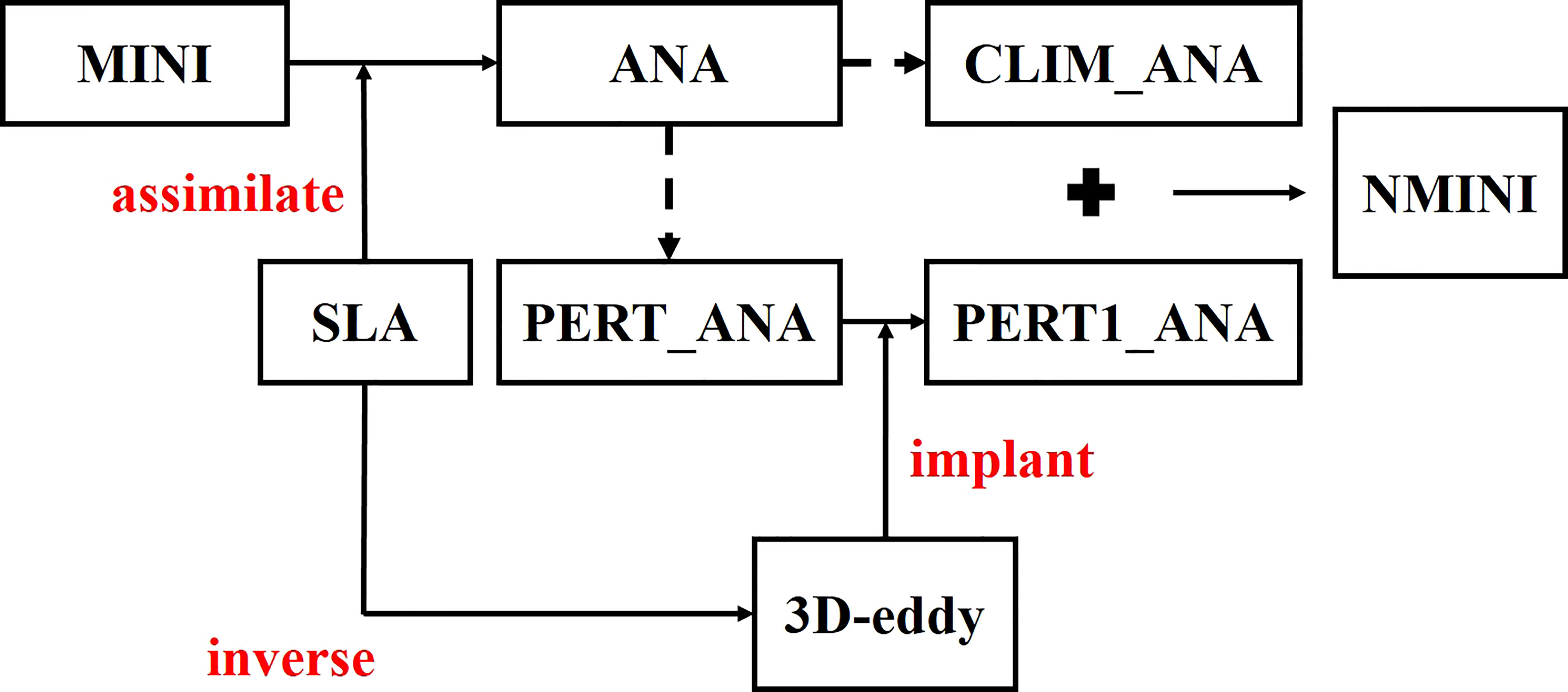
Figure 1 The diagrams of the vortex-implantation.

where V, x and y represent the currents of PERT1_ANA, the constructed 3D eddy and PERT_ANA, and EP is a ratio coefficient defined as:

$\begin{array}{ll}\text{EP}=1-{\text{e}}^{-{\left(\frac{r}{R_0}-2.5\right)}^8}& (23)\end{array}$

The values of EP regarding to the radius are shown in Figure 2. Based on Eq. (23) and the values of EP, the current field in the PERT_ANA is replaced by the retrieved current field of 3D eddy within 1.25 times eddy radius, and keeps unchanged beyond the 2 times eddy radius. It is a transitional region between the 1.25 and 2 times eddy radius to avoid an abrupt change of the current field. Finally, the PERT1_ANA is recombined with the CLIM_ANA to generate a new model initial field (denoted as NMINI) for eddy forecast.

FIGURE 2

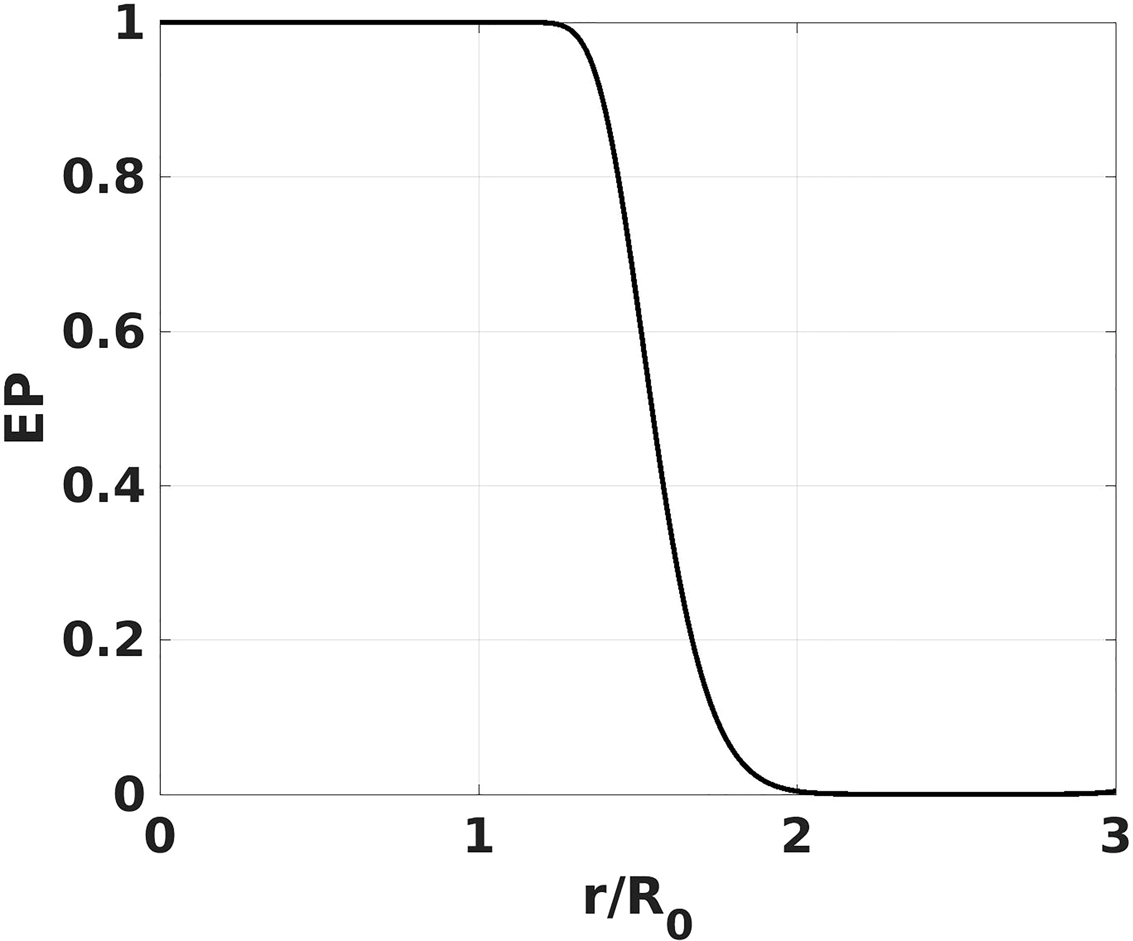
Figure 2 The function distribution of the implantation proportion coefficient EP of the 3D eddy.

Design of observational system simulation experiment (OSSE)

The purpose of OSSE is to assess the influence of an observational system or a forecast technique on the forecast skill, in which the “true” state is obtained from the model simulation or other mathematic ways (Arnold and Dey, 1986; Masutani et al., 2010). Before performing the OSSE, the 3D eddy should be constructed first because the mesoscale eddies could not be generated automatically by the free run under idealized model setting of ROMS. Here, two idealized 3D eddies including the warm and cold eddies were constructed separately for the OSSEs through the theoretical formulas (17)-(21). The η(r) and J(z) of the idealized 3D eddies are calculated using (18) and (19), in which the related parameters are set as follows: R_{0 =}50km, η₀ = ± 0.3m, N=0.008, θ₀ =π, k=(3π/2- θ₀ )/1800, H_{0 =}10 and H_ave =1, and the integral range in (19) is from sea surface to 1800m depth. The parameters for the constructions of the idealized warm and cold eddies are the same except for the sign of η₀ , which “+” represents the warm eddy and “-” represents the cold eddy. The profile of $\overline{\rho }$ is calculated using the T/S profile from the initial field of the experiment. The potential temperature of the idealized 3D eddies is calculated using a simplified state equation of sea water ρ=ρ₀(1−αT) , in which ρ₀ is 1025kg/m³ and α is 0.0003°C^-1, The salinity of the idealized 3D eddies is set to a constant of 34 psu. Figure 3 shows the vertical structure of J(z) of the idealized 3D eddies, and Figure 4 shows the 3D ρ^′ , potential temperature anomaly, u and v of the idealized 3D warm eddy.

FIGURE 3

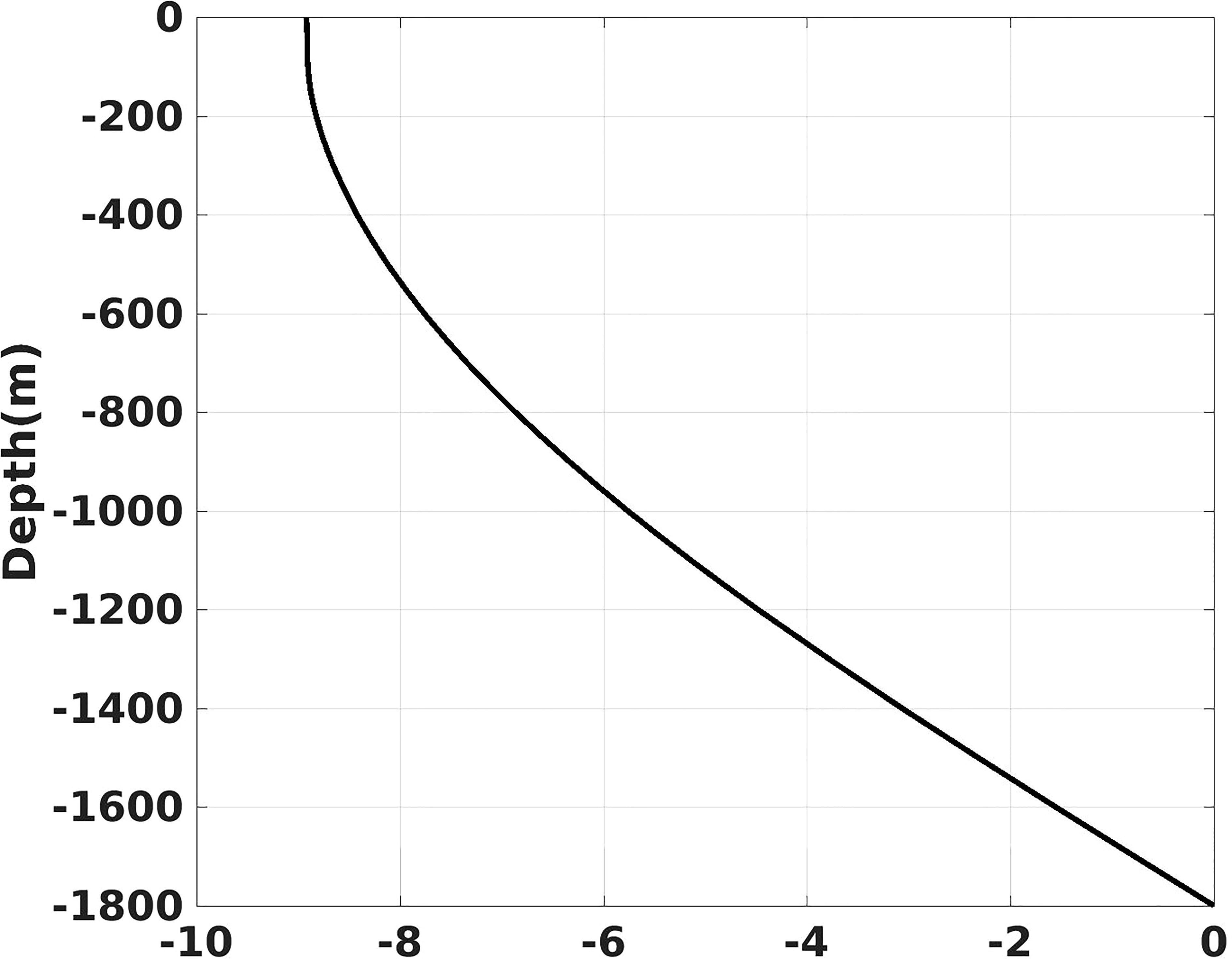
Figure 3 The vertical structure function J(z) of potential density of the idealized 3D eddy.

FIGURE 4

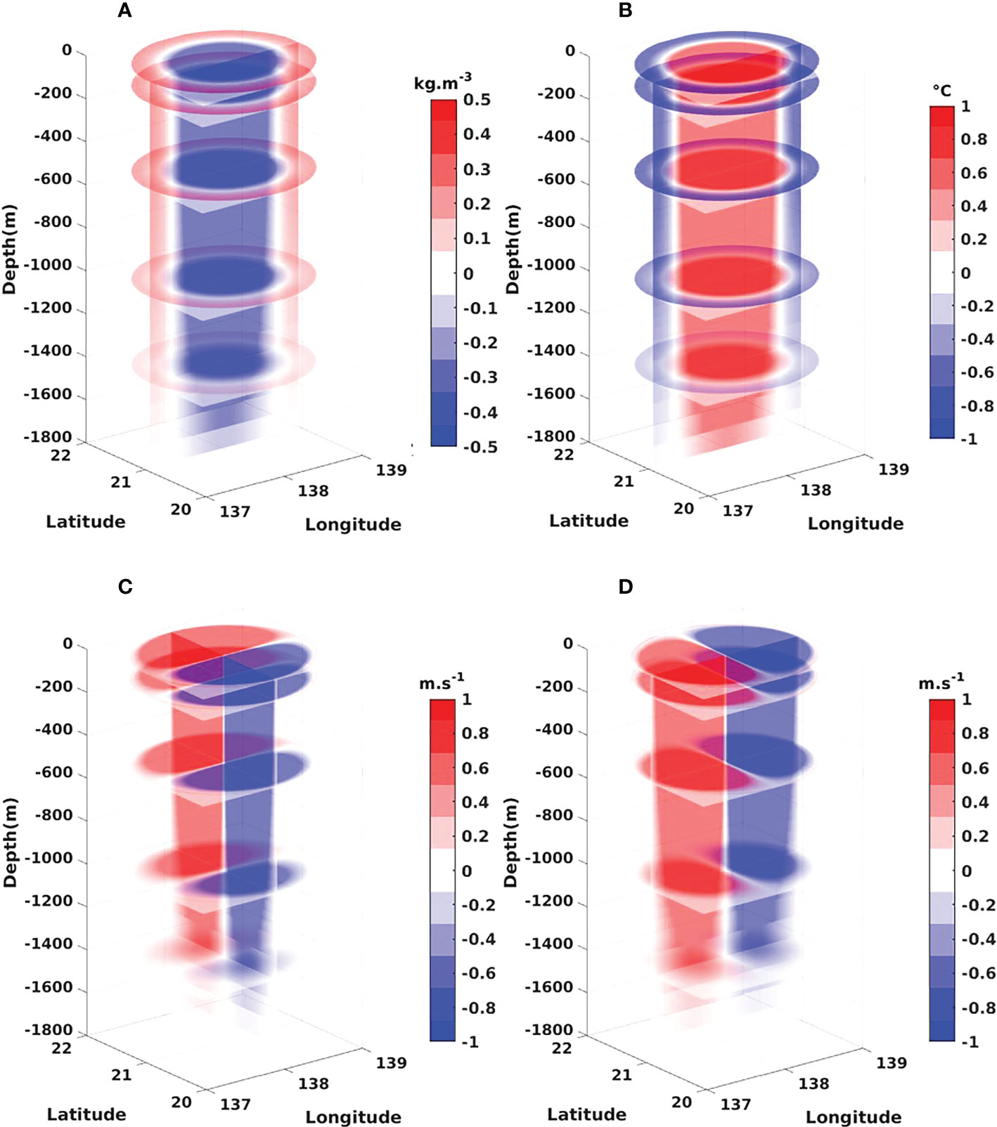
Figure 4 The 3D fields of potential density anomaly (A), potential temperature anomaly (B), current u-component (C) and current v-component (D) of the idealized 3D warm eddy.

The first step of the OSSEs is to generate the “true” state. A 30-day free run is conducted first to get a background field with steady westward current of u=-0.1m/s. Then, the SLA, temperature anomaly and current of the idealized 3D warm or cold eddy constructed before are added into the background field at the location 138°E, 21°N, followed by another 52-day simulation, which denotes as the “true” state run. The results between the 20^th to 52^th (33 days) day from the “true” state run are chosen as the “true” state for the OSSEs (Figure 5). Based on the background field, five experiments are designed for the OSSEs (Table 2). In the first pair of experiments (DASLA_W and DASLA_C), only the SLAs in the model domain obtained from the two “true” states are assimilated. In the second pair of experiments (ED_BOG_W and ED_BOG_C), the VISTEMP scheme is applied, of which the implanted 3D eddies is retrieved as follows: 1) the η(r) of the implanted 3D eddies is obtained from the SLA of the “true” state, 2) the parameters N and f of J(z) are calculated based on the mean T/S and location of the “true” 3D eddies at the implanting moment, and 3) the other parameters are set as follows to fit the vertical structure of “true” 3D eddies at the implanting moment: k=π/18000, θ₀ =-1800k, H_{0 =}1/sin(θ₀ ), H_ave=0. The values of J(z) for the implanted 3D eddies are plotted in Figure 6, from which we can see that the implanted 3D eddies dissipates greatly below the depth of 200m comparing to the idealized 3D eddies. As indicated in Section 3, J(z) is the key to the accuracy of the implanted 3D eddy, and in practice the estimate of J(z) could exist considerable biases. Therefore, the fifth experiment (ED_BOG_W_2J) is designed to investigate the impact of the J(z) estimate biases on the eddy prediction by erroneously doubling the absolute values of J(z) below the depth of 200m in the ED_BOG_W. All the five experiments are initialized with the results from 30-day free run. The assimilation of SLA or the application of the VISTEMP scheme is carried out at 0000 UTC of each day for 3 days, followed by a 30-day eddy prediction, as schematically illustrated in Figure 5.

FIGURE 5

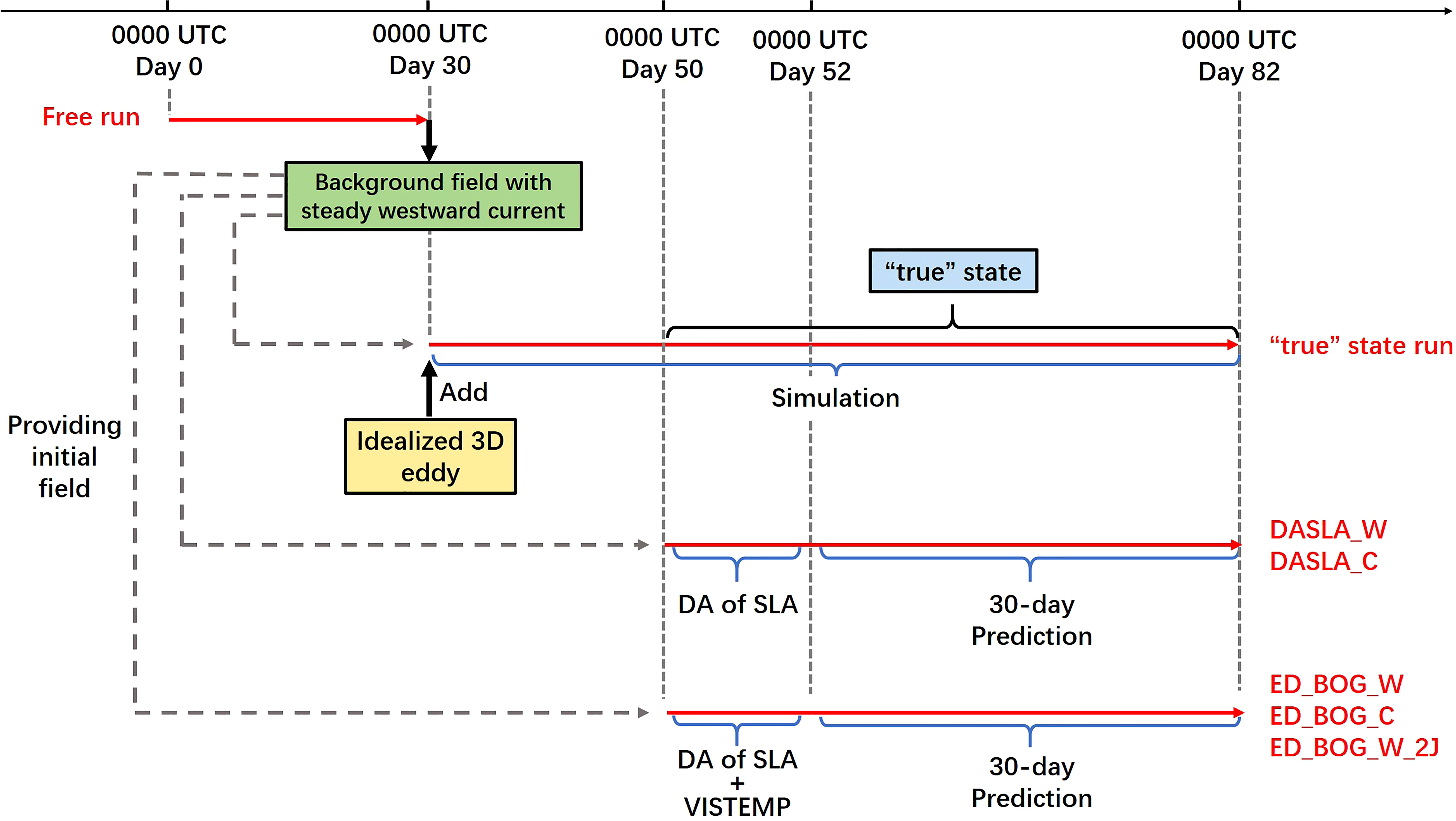
Figure 5 The flowchart of generation of “true” state and idealized prediction experiments.

TABLE 2

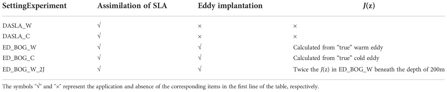
Table 2 The design of idealized prediction experiment.

FIGURE 6

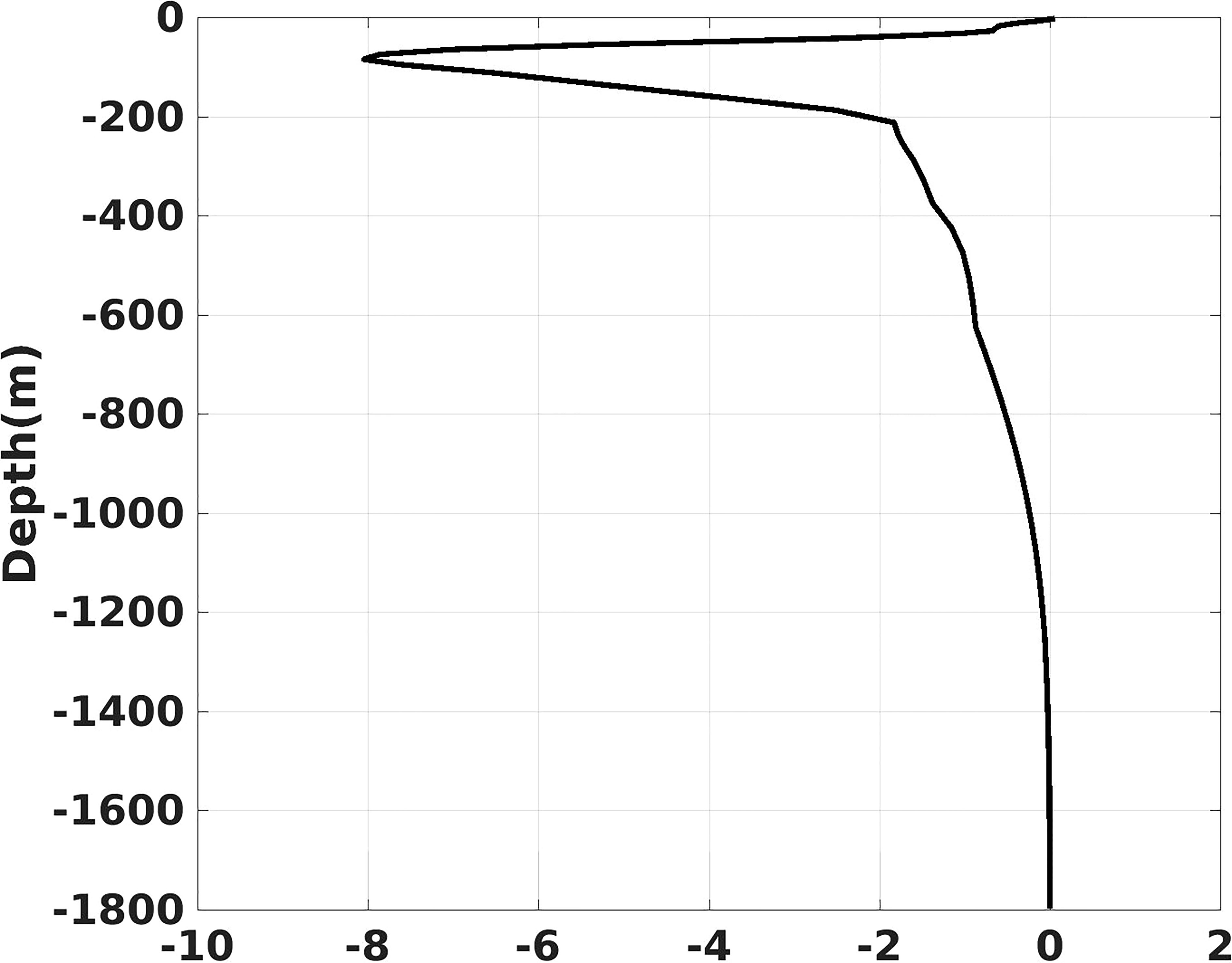
Figure 6 The vertical structure function J(z) of potential density of the implanted 3D eddy.

Results and discussion

The evaluation of eddy prediction

For the evaluation of eddy prediction, the Okubo-Weiss (OW) method is applied to the detection of eddies in the predicted fields. The feature variables, including the track, eddy center SLA (ECSLA), 0-500m averaged relative vorticity (RV), sea surface eddy kinetic energy (SSEKE), amplitude, rotation speed (ROS), size, and zonal/meridional moving speeds (mu and mv) are selected for the evaluation. Figure 7 shows the sea surface current and the vertical cross sections of u, v and temperature from “true” 3D warm eddy, DASLA_W and ED_BOG_W at the 10^th day. For the “true” 3D warm eddy, the sea surface current presents an asymmetrical distribution that is stronger in the south and weaker in the north, which is attributed to the westward background current (Figure 7A); the vertical sections of u and v show that the depth of the “true” 3D warm eddy reaches down to 1000m depth (Figures 7D, G). For DASLA_W, the sea surface current is much weaker than that in the “true” 3D warm eddy (Figure 7B), and the assimilation of SLA can only adjust the current down to a depth of about 300m beneath the sea surface through the B-matrix and dynamical constrains in the 3DVAR system (Figures 7E, H). For ED_BOG_W, the vertical structure of predicted eddy in terms of current field ((Figures 7C, F, I) and temperature field is very close to the “true” 3D warm eddy (Figures 7J, K, L). The results from the experiments for 3D cold eddy are similar (not shown).

FIGURE 7

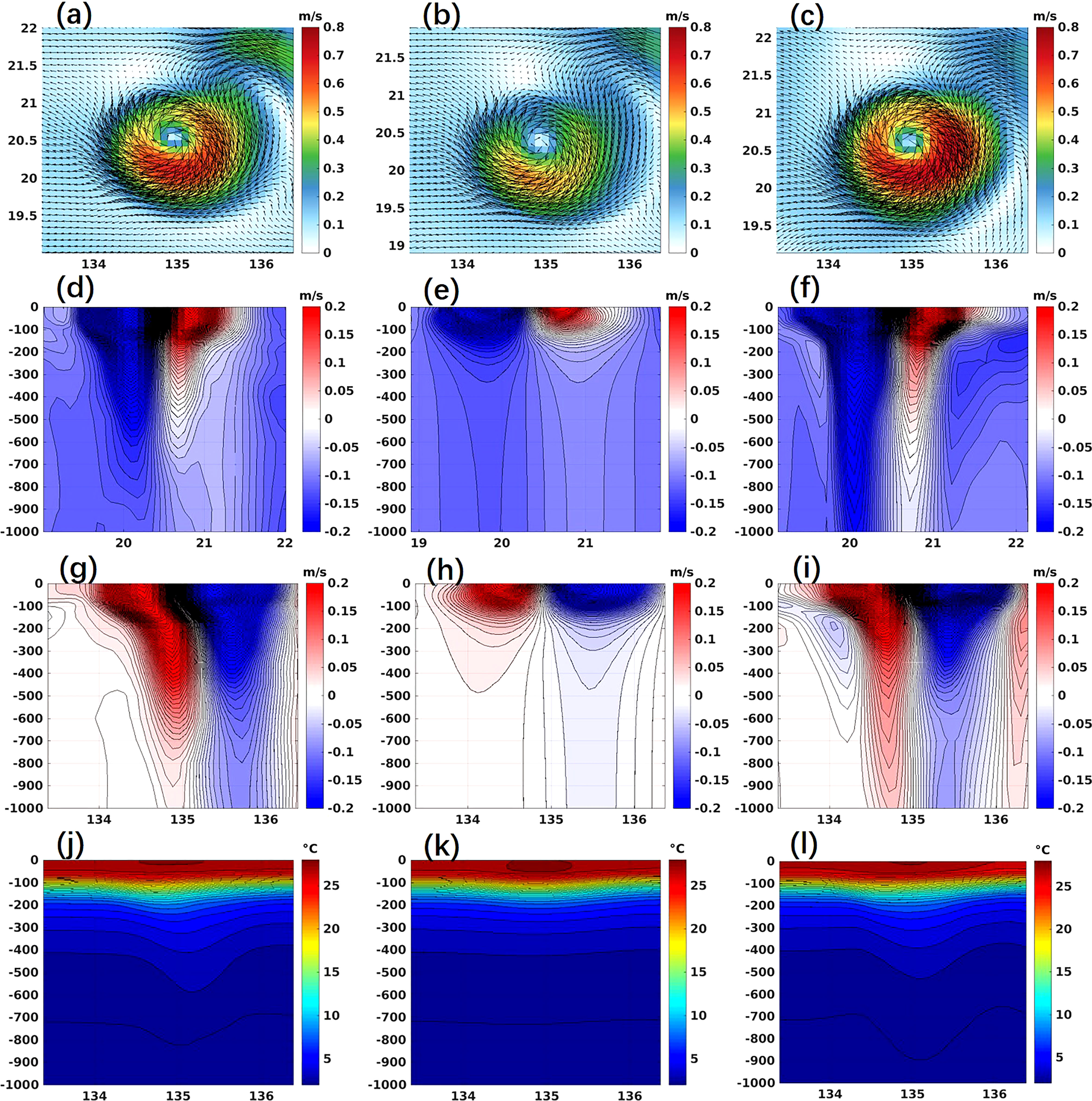
Figure 7 The (A–C) sea surface current, eddy center-crossed section of (D–F) u, (G–I) v component of current and (J–L) temperature on 10th prediction day from (A, D, G, J) “true” 3D warm eddy, (B, E, H, K) DASLA_W and (C, F, I, L) ED_BOG_W of the idealized experiment, in which the color and arrows in (A–C) represent the current speed and direction, respectively.

The 30-day averaged prediction biases of eddy feature variables for the warm and cold eddies are listed in Tables 3 and 4, respectively. The implement of the VISTEMP significantly reduces the biases of the track, ECSLA, RV, SSEKE, amplitude and ROS of the predicted warm eddy, but has little effect on biases of size, mu and mv. Similar results are obtained for the experiment with a cold eddy (ED_BOG_C); in addition, the bias of size is also reduced. Figures 8 and 9 show the eddy tracks from “true” eddies and different experiments as well as the time series of the prediction biases of eddy feature variables for different experiments. The “true” warm (cold) eddy moves southwestward (northwestward) under the influences of background current and β-effect (Chelton et al., 2011; Liu et al., 2012). The track predicted by DASLA_W (DASLA_C) presents a significant southern (northern) deviation, which is corrected by the VISTEMP scheme in ED_BOG_W (ED_BOG_C) (Figures 8 and 9A, B). The eddy size is underestimated (overestimated) in DASLA_W (DASLA_C), while it is overestimated in ED_BOG_W (Figure 8I) and well predicted in ED_BOG_C (Figure 9I). Generally, the larger the eddy scale, the further poleward the eddy moves due to the stronger β-effect (Chelton et al., 2011). It is obvious that, while DASLA_W and DASLA_C significantly underestimate the ECSLA, RV, SSEKE, amplitude and ROS of the eddy, ED_BOG_W and ED_BOG_C provide a much better prediction of the eddy regarding to these feature variables (Figures 8/9E, F, G, H, J).

TABLE 3

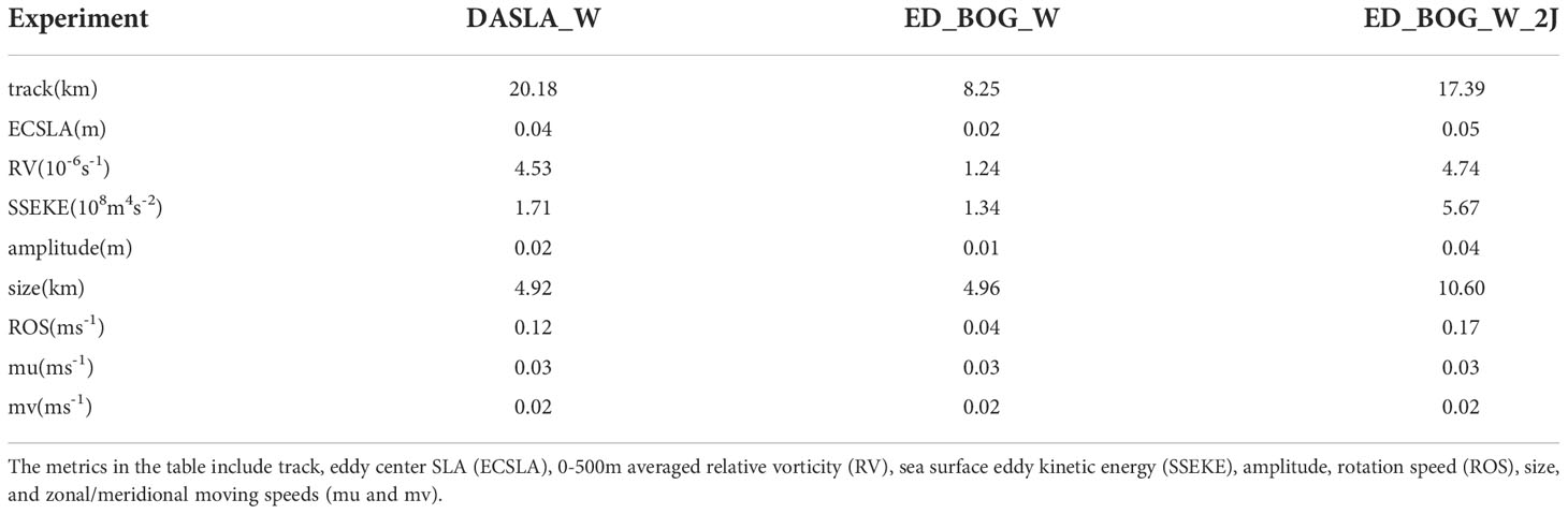
Table 3 The 30-day mean prediction error of the eddy feature variables from experiment DASLA_W, ED_BOG_W and ED_BOG_2J.

TABLE 4

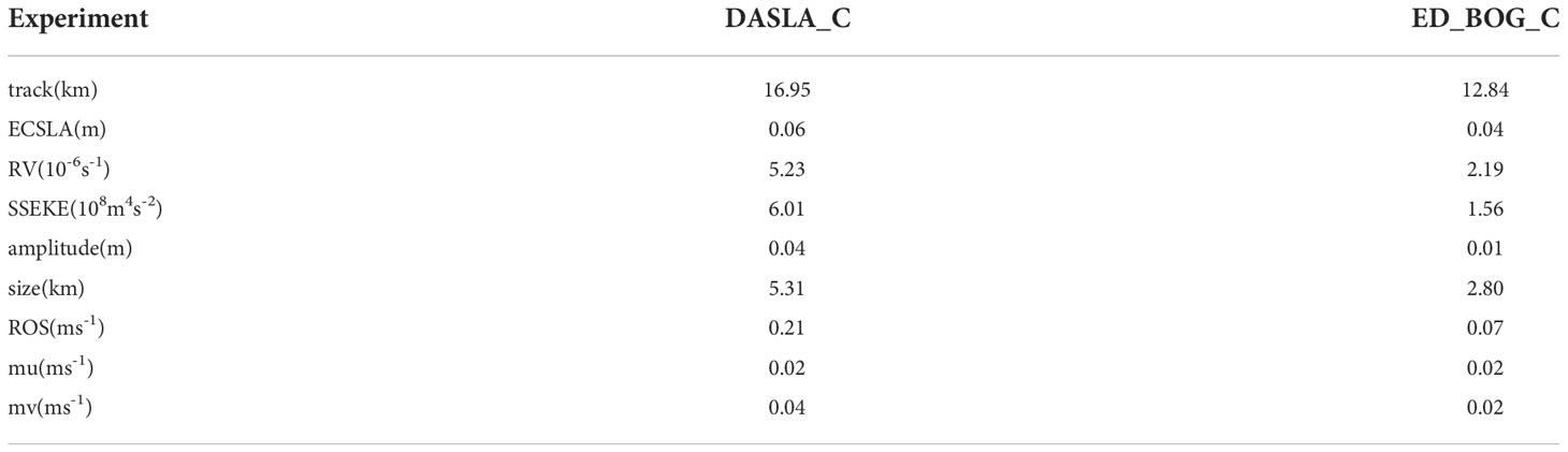
Table 4 The same as Table 3 except for the DASLA_C and ED_BOG_C.

FIGURE 8

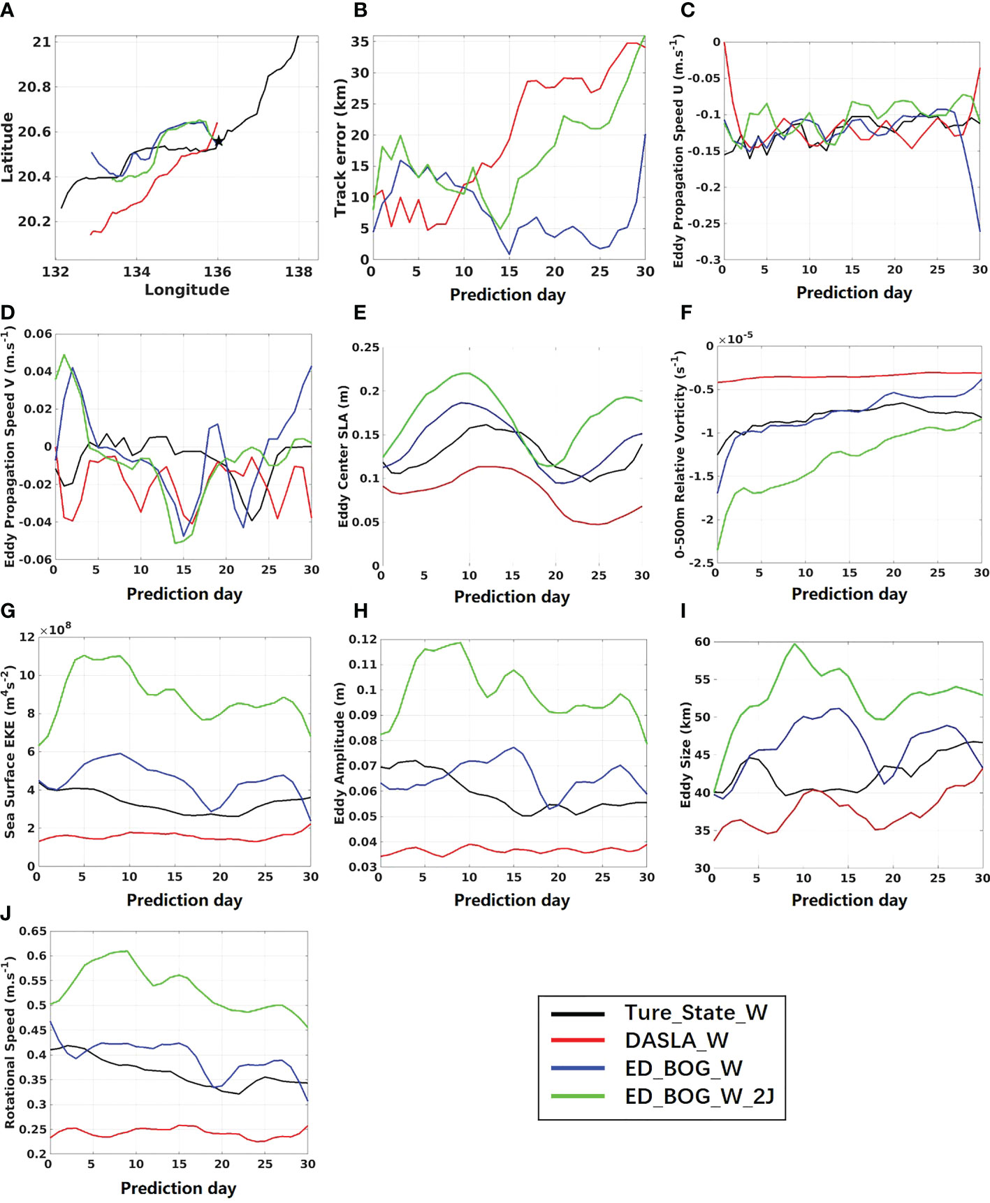
Figure 8 The (A) track, time series of (B) track prediction error, (C) mu, (D) mv, (E) strength, (F) RV, (G) SSEKE, (H) amplitude, (I) scale and (J) ROS of predicted eddy from “true” warm eddy, DASLA_W, ED_BOG_W and ED_BOG_2J during the prediction period.

FIGURE 9

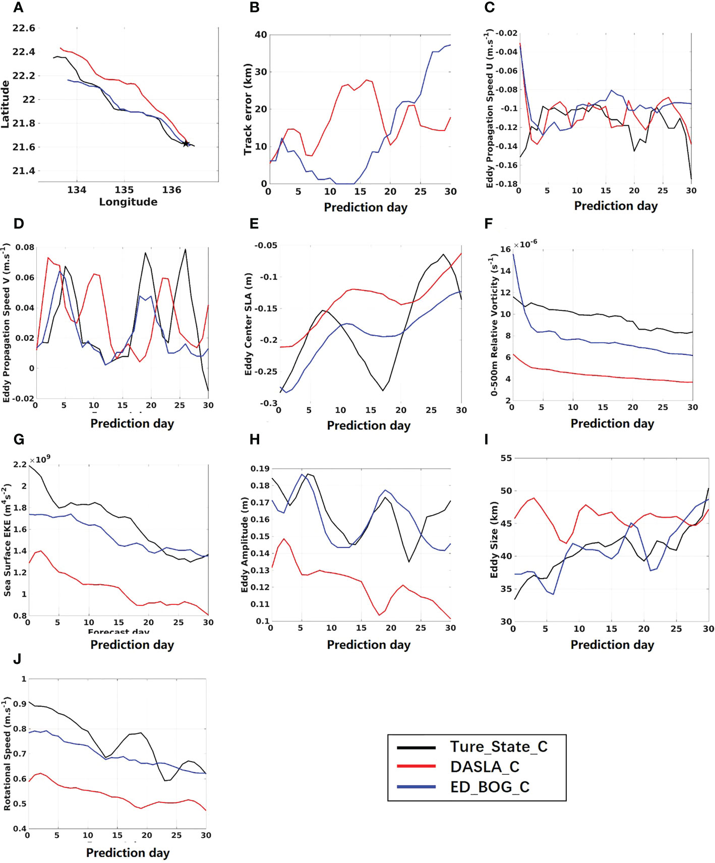
Figure 9 The (A) track, time series of (B) track prediction error, (C) mu, (D) mv, (E) strength, (F) RV, (G) SSEKE, (H) amplitude, (I) scale and (J) ROS of predicted eddy from “true” cold eddy, DASLA_C and ED_BOG_C during the prediction period.

It should be aware that the VISTEMP is developed under the assumption that the mesoscale eddies are upright in the ocean. In the real ocean, the mesoscale eddies are not always upright, and may have a “lean” in the most dynamic regions (Poulsen et al., 2019). The decomposition that treats the mesoscale eddies as an upright body is not perfect, from which the constructed 3D eddy is only a proxy of the real one. Therefore, the effect of the VISTEMP for lean eddies may be limited. Actually, the predicted eddy using the VISTEMP (Figures 8F, I) also shows a lean in vertical structure, suggesting that the upright vertical structure of the implanted 3D eddy could be adjusted to a leaning one that is close to the “true” state with model integration.

The impact of the estimate biases of the implanted 3D warm eddy vertical structure on the mesoscale eddy prediction

As shown in Figures 8A, B, the eddy track predicted by ED_BOG_W_2J has larger errors after 15 days than that by ED_BOG_W, which could be due to errors in the predicted movement speed (Figures 8C, D). Regarding to the other feature variables, including ECSLA, RV, SSEKE, amplitude, size, ROS, ED_BOG_2J generally overestimates them compared with ED_BOG_W. For instance, the absolute value of RV from ED_BOG_2J, which is a key measurement for the strength of an eddy, is much larger than that from ED_BOG_W, indicating a stronger eddy predicted by ED_BOG_W _2J; moreover, the absolute value of RV decreases with forecast time in both ED_BOG_W _2J and ED_BOG_W, suggesting that the eddy is dissipated gradually (Figure 8F).

The results show that the key to a good performance in eddy prediction by the VISTEMP is the accuracy of retrieving the implanted 3D eddy from SLA, which mainly depends on the accuracy of J(z) calculation. In the ideal experiment, the accuracy can be guaranteed because the J(z) can be easily fitted to the vertical structure of the “true” 3D eddy in the OSSEs by adjusting the unknown parameters in the theoretical formulas. However, the J(z) for eddies in the real ocean can only be obtained through a composite analysis based on the historical satellite-derived SLA and T/S profiles (e.g. Argo T/S profile), in which the accuracy of J(z) may be somewhat reduced. Therefore, how to make the bias in the J(z) calculation within an acceptable range is the key to the successful application of the VISTEMP in the real mesoscale eddy prediction.

Summary

In this study, a vortex-implanted initialization scheme for the mesoscale eddy prediction (VISTEMP) is developed. With VISTEMP, a 3D eddy is implanted into the model initial field by replacing the original current field with the one derived from SLA, generating a new initial field that provides a more accurate description of mesoscale eddy for prediction. A set of OSSEs based on the idealized model setting are conducted to evaluate the effect of the VISTEMP on the prediction of mesoscale eddies. The results show that the application of the VISTEMP improves the prediction for mesoscale eddies in terms of track, ECSLA, vertical structure and so on, as compared to the experiment that only assimilates SLA. The results of OSSEs also indicate that the improvement of eddy prediction is largely influenced by the estimate biases of the vertical structure in the construction of the 3D eddy.

This study provides an innovative method for the mesoscale eddies’ prediction, which could have great potential application in operational services of the marine environments. However, more experiments and analysis need to be carried out before the practical application, such as the OSSEs for real simulation and the application in real hindcast. This will be our work in the future.

Data availability statement

The raw data supporting the conclusions of this article will be made available by the authors, without undue reservation.

Author contributions

YZ developed the vortex-implanted initialization scheme, designed and conducted the forecast experiments, validated and analyzed the experiment results, wrote the manuscript. SP provided the original idea, offered suggestions, polished up the manuscript. YL offered suggestions. All authors contributed to the article and approved the submitted version.

Funding

This work was jointly supported by the National Natural Science Foundation of China (Grant Nos. U20A20105, 41931182, 41890851 and U21A6001), Guangdong Special Support Program (Grant No.2019BT2H594), Guangxi Key Laboratory of Marine Disaster in the Beibu Gulf, Beibu Gulf University (Grant No.2021KF01), the Strategic Priority Research Program of the Chinese Academy of Sciences (Grant No. XDA19060503), and the Independent Research Project Program of State Key Laboratory of Tropical Oceanography under contract (Grant No.LTOZZ2004). The authors gratefully acknowledge the use of the HPCC at the South China Sea Institute of Oceanology, Chinese Academy of Sciences.

Conflict of interest

The authors declare that the research was conducted in the absence of any commercial or financial relationships that could be construed as a potential conflict of interest.

Publisher’s note

All claims expressed in this article are solely those of the authors and do not necessarily represent those of their affiliated organizations, or those of the publisher, the editors and the reviewers. Any product that may be evaluated in this article, or claim that may be made by its manufacturer, is not guaranteed or endorsed by the publisher.

References

Arnold C. P., Dey C. H. (1986). Observing-systems simulation experiments: past, present, and future. Bull. Am. Meteorol. Soc. 67, 687–695. doi: 10.1175/1520-0477(1986)067<0687:OSSEPP>2.0.CO;2

CrossRef Full Text | Google Scholar

Chaigneau A., Pizarro O. (2005). Eddy characteristics in the eastern South pacific. J. Geophys. Res. Oceans 110 (C8), 207–229. doi: 10.1029/2004JC002815

CrossRef Full Text | Google Scholar

Chaigneau A., Pizarro O. (2011). Eddy characteristics in the eastern South pacific. J.Geophys. Res. Oceans 110 (C8), 207–229. doi: 10.1029/2004JC002815.

CrossRef Full Text | Google Scholar

Chassignet E. P., Hurlburt H. E., Metzger E. J., Smedstad O. M., Cummings J. A., Halliwell G. R., et al. (2009). US GODAE: Global ocean prediction with the HYbrid coordinate ocean model (HYCOM). Oceanography 22 (2), 64–75. doi: 10.5670/oceanog.2009.39

CrossRef Full Text | Google Scholar

Chelton D. B., Freilich M. H., Esbensen S. K. (2000). Satellite observations of the wind jets off the pacific coast of central america. part I: Case studies and statistical characteristics, Mon. Weather Rev. 128, 1993–2018. doi: 10.1175/1520-0493(2000)128<1993:SOOTWJ>2.0.CO;2

CrossRef Full Text | Google Scholar

Chelton D. B., Schlax M. G., Samelson R. M. (2011). Global observations of nonlinear mesoscale eddies. Prog. Oceanogr. 91 (2), 167–216. doi: 10.1016/j.pocean.2011.01.002

CrossRef Full Text | Google Scholar

Chelton D. B., Schlax M. G., Samelson R. M., Szoeke R. A. D. (2007). Global observations of large oceanic eddies. Geophys. Res. Lett. 34 (15), 87–101. doi: 10.1029/2007GL030812

CrossRef Full Text | Google Scholar

Daley R. (1993). Atmospheric data analysis (New York: Cambridge University Press).

Google Scholar

Debreu L. P., Marchesiello P., Penven P., Cambon G. (2012). Two way nesting in split explicit ocean models: Algorithms, implementation and validation. Ocean Model. 49-50, 1–21. doi: 10.1016/j.ocemod.2012.03.003

CrossRef Full Text | Google Scholar

Dong C., Lin X., Liu Y., Nencioli F., Chao Y., Guan Y., et al. (2012). Three-dimensional oceanic eddy analysis in the southern California bight from a numerical product. J. Geophys. Res. 117, C00H14. doi: 10.1029/2011JC007354

CrossRef Full Text | Google Scholar

Flierl G. R. (1987). Isolated eddy models in geophysics. Ann. Rev. Fluid Mech. 19, 493–530. doi: 10.1146/annurev.fl.19.010187.002425

CrossRef Full Text | Google Scholar

Graham A. (1981). Kronecker Products and matrix calculus with applications (Chichester, UK: Ellis Horwood).

Google Scholar

Halo I., Penven P., Backeberg B. C., Ansorge I., Shillington F. A., Roman R. (2014). Mesoscale eddy variability in the southern extension of the East Madagascar current: Seasonal cycle, energy conversion terms, and eddy mean properties. J. Geophys. Res. Ocean. 119 (10), 7324–7356. doi: 10.1002/2014JC009820

CrossRef Full Text | Google Scholar

Isern-Fontanet J. E., Font J., Garcia-Ladona E., Emelianov M., Millot C., Taupier-Letage I. (2004). Spatial structure of anticyclonic eddies in the Algerian basin (Mediterranean Sea) analyzed using the okubo–Weiss parameter. Deep-Sea Res. II 51, 3009–3028. doi: 10.1016/j.dsr2.2004.09.013

CrossRef Full Text | Google Scholar

Isern-Fontanet J. E., Garcia-Ladona E., Font J. (2003). Identification of marine eddies from altimetric maps. J. Atmos. Ocean. Technol. 20, 772–778. doi: 10.1175/1520-0426(2003)20<772:IOMEFA>2.0.CO;2

CrossRef Full Text | Google Scholar

Isern-Fontanet J. E., Garcia-Ladona E., Font J. (2006). Vortices of the Mediterranean Sea: An altimetric perspective. J. Phys. Oceanogr. 36, 87–103. doi: 10.1175/JPO2826.1

CrossRef Full Text | Google Scholar

Kloosterziel R. C. (1990). On the large-time asymptotics of the diffusion equation of infinite domains. J. Eng. Math. 24, 213–236. doi: 10.1007/BF00058467

CrossRef Full Text | Google Scholar

Kurihara Y., Bender M. A., Ross R. J. (1993). An initialization scheme of hurricane models by vortex specification. Mon. Weather Rev. 121 (7), 2030. doi: 10.1175/1520-0493(1993)121<2030:AISOHM>2.0.CO;2

CrossRef Full Text | Google Scholar

Large W. G., McWilliams J. C., Doney S. C. (1994). Oceanic vertical mixing: A review and a model with a nonlocal boundary layer parameterization. Rev. Geophys. 32 (4), 63–403. doi: 10.1029/94RG01872

CrossRef Full Text | Google Scholar

Lee H., Chang P. H., Kang K., Kang H. S., Kim Y. (2018). Assessment of ocean surface current forecasts from high resolution global seasonal forecast system version 5. Ocean Polar Res. 40 (3), 99–114. doi: 10.4217/OPR.2018.40.3.099

CrossRef Full Text | Google Scholar

Liang J. H., Mcwilliams J. C., Kurian J., Colas F., Wang P., Uchiyama Y. (2012). Mesoscale variability in the northern tropical pacific: Forcing mechanisms and eddy properties. J. Geophys. Res. Atmos. 117 (C7), 165–165. doi: 10.1029/2012JC008008

CrossRef Full Text | Google Scholar

Li Z. J., Chao Y., Mcwilliams J. C., IDE K. (2008a). A three-dimensional variational data assimilation scheme for the regional ocean modeling system. J. Atmos. Ocean. Technol. 25, 2074–2090. doi: 10.1175/2008JTECHO594.1

CrossRef Full Text | Google Scholar

Li Z. J., Chao Y., Mcwilliams J. C., IDE K. (2008b). A three-dimensional variational data assimilation scheme for the regional ocean modeling system: Implementation and basic experiments. J. Geophys. Res. 113, C05002. doi: 10.1029/2006JC004042

CrossRef Full Text | Google Scholar

Liu Y., Dong C. M., Guan Y. P. (2012). Eddy analysis in the subtropical zonal band of the north pacific ocean. Deep Sea Res. Part I: Oceanogr. Res. Pap. 68, 54–67. doi: 10.1016/j.dsr.2012.06.001

CrossRef Full Text | Google Scholar

Martin M. J., Hines A., Bell M. J. (2007). Data assimilation in the FOAM operational short-range ocean forecasting system: a description of the scheme and its impact. Q. J. R. Meteorol. Soc. 133, 981–995. doi: 10.1002/qj.74

CrossRef Full Text | Google Scholar

Masutani M., Woollen J. S., Lord S. J., Emmitt G. D., Kleespies T. J. (2010). Observing system simulation experiments at the national centers for environmental prediction. J. Geophys. Res.: Atmos. 115, D07101. doi: 10.1029/2009JD012528.

CrossRef Full Text | Google Scholar

Morrow R., Birol F., Griffin D., Sudre J. (2004). Divergent pathways of cyclonic and anti-cyclonic ocean eddies. Geophys. Res. Lett. 31 (31), 357–370. doi: 10.1029/2004GL020974

CrossRef Full Text | Google Scholar

Orlanski I. (1976). A simple boundary-condition for unbounded hyperbolic flows. J. Comput. Phys. 21 (3), 251–269. doi: 10.1016/0021-9991(76)90023-1

CrossRef Full Text | Google Scholar

Parrish D. F., Derber J. C. (1992). The national meteorological center's spectral statistical-interpolation analysis system. Mon. Weather Rev. 120 (8), 1747–1763. doi: 10.1175/1520-0493(1992)120<1747:TNMCSS>2.0.CO;2

CrossRef Full Text | Google Scholar

Peng S. Q., Zhu Y. H., Li Z. J., Li Y. N., Xie Q., Liu S. J., et al. (2019). Improving the real-time marine forecasting of the northern south China Sea by assimilation of gliderobserved T/S profiles. Sci. Rep 9, 17845, . doi: 10.1038/s41598-019-54241-8

PubMed Abstract | CrossRef Full Text | Google Scholar

Penven P., Debreu L., Marchesiello P., McWilliams J. C. (2006). Evaluation and application of the ROMS 1-way embedding procedure to the central California upwelling system. Ocean Model. 12, 157–187. doi: 10.1016/j.ocemod.2005.05.002

CrossRef Full Text | Google Scholar

Poulsen M. B., Jochum M., Maddison J. R., Marshall D., Nuterman R. (2019). A geometric interpretation of southern ocean eddy form stress. J. Phys. Oceanogr. 49 (10), 2553–2070. doi: 10.1175/JPO-D-18-0220.1

CrossRef Full Text | Google Scholar

Raymond W. H., Kuo H. L. (1984). A radiation boundary-condition for multi-dimensional flows. Q. J. R. Meteorol. Soc. 110, 535–551. doi: 10.1002/qj.49711046414

CrossRef Full Text | Google Scholar

Sandhya K. G., Murty P. L. N., Deshmukh A. N., Nair T. M. B., Shenoi S. S. C. (2018). An operational wave forecasting system for the east coast of India. Estuar. Coast. Shelf Sci. 202, 114–124. doi: 10.1016/j.ecss.2017.12.010

CrossRef Full Text | Google Scholar

Shchepetkin A. F., McWilliams J. C. (2003). A method for computing horizontal pressure-gradient force in an oceanic model with a nonaligned vertical coordinate. J. Geophys. Res.: Ocean. 108 (C3), 35.1–35.4. doi: 10.1029/2001JC001047

CrossRef Full Text | Google Scholar

Shchepetkin A. F., McWilliams J. C. (2005). The regional oceanic modeling system (ROMS): a split explicit, free surface, topography following coordinate oceanic model. Ocean Model. 9 (4), 347–404. doi: 10.1016/j.ocemod.2004.08.002

CrossRef Full Text | Google Scholar

Shriver J. F., Hurlburt H. E., Smedstad O. M., Wallcraft A. J., Rhodes R. C. (2007). 1/32° real-time global ocean prediction and value-added over 1/16° resolution. J. Mar. Syst. 65, 3–26. doi: 10.1016/j.jmarsys.2005.11.021

CrossRef Full Text | Google Scholar

Usui N., Lshizaki S., Fujii Y., Tsujino H., Yasuda T., Kamachi M. (2006). Meteorological research institute multivariate ocean variational estimation (MOVE) system: Some early results. Adv. Space Res. 37, 806–822. doi: 10.1016/j.asr.2005.09.022

CrossRef Full Text | Google Scholar

Wang G., Su J. L., Qi Y. Q. (2005). Advances in studying mesoscale eddies in south China Sea. Adv. Earth Sci. 20 (8), 882–886. doi: 10.11867/J.ISSN.1001-8166.2005.08.0882.

CrossRef Full Text | Google Scholar

Wang H., Liu N., Li B. X., Li X. (2014). An Overview of Ocean Predictability and Ocean Ensemble Forecast. Advances in Earth Science 29 (11), 1212–1225 (In Chinese).

Google Scholar

Xu L. X., Xie S. P., McClean J. L., Liu Q. Y., Sasaki H. (2016). Observing mesoscale eddy effects on mode-water subduction and transport in the north pacific. Nat. Commun. 7, 10505. doi: 10.1038/ncomms10505

PubMed Abstract | CrossRef Full Text | Google Scholar

Yang G., Wang F., Li Y., Lin P. (2013). Mesoscale eddies in the northwestern subtropical pacific ocean: statistical characteristics and three-dimensional structures. J. Geophys. Res. 118, 1–20. doi: 10.1002/jgrc.20164

CrossRef Full Text | Google Scholar

Zhang Z. W., Tian J., Qiu B., Zhao W., Chang P., Wu D., et al. (2016). Observed 3D structure, generation, and dissipation of oceanic mesoscale eddies in the south China Sea. Sci. Rep. 6, 24349. doi: 10.1038/srep24349

PubMed Abstract | CrossRef Full Text | Google Scholar

Zhang Z. G., Zhang Y., Wang W., Huang R. X. (2013). Universal structure of mesoscale eddies in the ocean. Geophys. Res. Lett. 40, 3677–3681. doi: 10.1002/grl.50736

CrossRef Full Text | Google Scholar

Zhu Y. H., Li Y. N., Peng S. Q. (2020). The track and accompanying Sea wave forecasts of the supertyphoon mangkhut, (2018) by a real-time regional forecast system. J. Atmos. Ocean. Technol. 37 (11), 2075–2084. doi: 10.1175/JTECH-D-19-0196.1

CrossRef Full Text | Google Scholar

Appendix

1) The definition of mesoscale eddies’ feature variables.

The feature variables of mesoscale eddies in this study are defined as below. a) Track: the moving track of the eddy represented by the longitude and latitude of an eddy center; b) Radius (km): The radius of a circle with equal area surrounded by the edge of an eddy; c) Rotation speed (ms^-1): The maximum of the averaged speed along each closed streamline of an eddy (Chelton et al., 2011); d) Sea surface eddy kinetic energy (m⁴s^-2): sea surface eddy kinetic energy of the mesoscale eddy SSEKE, which is represented as

$\begin{array}{ll}\text{SSEKE}=\frac{S*\left(u^2+v^2\right)}{2}& (1)\end{array}$

In which S is the area of the mesoscale eddy at sea surface; e) Amplitude (m): The height difference between the eddy center and the averaged SSH along the eddy edge (Chelton et al., 2011); f) Size (km): The mean distance between the eddy center and the streamline where the rotation speed located (Chelton et al., 2011); g) Relative vorticity (s^-1): sea surface relative vorticity Ω, which is represented as

$\begin{array}{ll}\text{Ω}=\frac{\partial v^{,}}{\partial x}-\frac{\partial u^{,}}{\partial y}& (2)\end{array}$

2) The detection of mesoscale eddies.

The detection method of mesoscale eddies used in this study is the Okubo-Weiss (OW, Chelton et al., 2007) method. The OW method define the area where the parameter W less than 2e×10^-12s^-2 as the area of the eddy (Chaigneau et al., 2011), in which the parameter W is defined as (2006; Isern-Fontanet et al., 2003):

$\begin{array}{ll}W=4\left(u_x^2+v_x{u}_y\right)& (3)\end{array}$

Several thresholds are defined for the eddy detection: The maximum and minimum radiuses of an eddy is 400km and 30km, respectively. The minimum amplitude is 0.02m and the minimum life period is 7 days.

The eddy should be numbered after detection. Penven (2006) proposes a dimensionless parameter that represents the similarity of eddies at different times. For two eddies e₁, e₂, the similarity parameter is defined as

$\begin{array}{ll}{X}_{e_1{e}_2}=\sqrt{{\left(\frac{\Delta L}{L_0}\right)}^2+{\left(\frac{\Delta R}{R_0}\right)}^2+{\left(\frac{\Delta \xi }{{\xi }_0}\right)}^2+{\left(\frac{\Delta Z}{Z_0}\right)}^2+{\left(\frac{\Delta A}{A_0}\right)}^2}& (4)\end{array}$

In which L₀ , R₀ , ξ₀ , Z₀ and A₀ represent the feature distance, feature radius, feature relative vorticity, feature mean SSH and feature amplitude, which are set to 15km, 100km, 10^-5s^-1, 0.1m and 0.1m, respectively. Δ represents the difference of feature variable between e₁, e₂. There are two rules in the determination of the eddy number: a) The two eddies with the minimum X_e1e2 are detected as the same eddy at different time; b) The moving speed of the eddy e₁/e₂ in a) should not beyond 0.3ms^-1.