Spatio-temporal nonconvex penalty adaptive chirp mode decomposition for signal decomposition of cross-frequency coupled sources in seafloor dynamic engineering

Electromagnetic field noise and clutter generated from the motion of ocean waves are the main obstacles in the research of magnetotelluric dynamic analysis, and it is difficult to extract the crossed instantaneous frequencies (IFs) of underwater electromagnetic detected (UEMD) data due to the limited resolution of the current time-frequency techniques. To alleviate this bottleneck issue, a new spatio-temporal nonconvex penalty adaptive chirp mode decomposition (STNP-ACMD) is originally proposed for separating each mono-component individually from a complicated multi-component with severely crossed IFs or overlapped components, in this paper. Specifically, the idea of a nonconvex penalty greedy strategy is incorporated into the vanilla ACMD method by using a recursive mode extraction scheme, and the fractional-order characteristic of the observation signal is also considered. Meanwhile, the spatio-temporal matrices were constructed elaborately and then applied to capture coupling characteristics and spatio-temporal relationships among all estimated mono-components. Eventually, a high-resolution adaptive time-frequency spectrum is obtained according to the IFs and instantaneous amplitudes (IAs) of each estimated mono-component. The effectiveness and practicability of the proposed algorithm were verified via simulated scenarios and velocity dynamic data of the seafloor from the South China Sea, compared with four state-of-the-art benchmarks.

1 Introduction

Underwater electromagnetic detected (UEMD) data with low frequency have a wide application prospect in deep-sea exploration and deep-sea magnetic field measurements such as oil and mineral exploration, underwater pipe-cable overhaul, fishery, navigation, positioning, ship testing, and anti-submarine demining, due to many merits including high accuracy, stability, and relatively small restrictions by hydrologic weather, and so on. However, the UEMD data with low frequency is susceptible to the electromagnetic noise induced by the ocean current, and the issue of frequency range overlap between UEMD data with low frequency and induced electromagnetic noise is becoming the main obstacle to improving the signal-to-noise ratio (SNR) of UEMD data since the signal recorded via the receiver is usually affected by different types of noise, such as electromagnetic field noise, clutter, and marine animals (Park et al., 2019; Nyqvist et al., 2020; Schwalenberg et al., 2020).

The UEMD data, such as radar-echo wave and ocean current sonar, usually exhibit non-stationary, time-varying, and multi-component characteristics, and those data (sound and signals) always contain useful information for engineering applications. Extracting or isolating the constituent modes from their complicated multi-dimensional or multi-component nature is a pivotal task for understanding the dynamic responses in seafloor engineering. Therefore, how to achieve accurate signal decomposition and represent the internal physical characteristics of a system has been a hot research topic.

1.1 Literature review

Over the past few years, multiple methods and studies have been adopted to alleviate this issue. For example, in 2013, MacLennan et al. proposed a flexible and practical denoising technique named equivalent source method (ESM) to remove the additional noise from multicomponent controlled-source electromagnetic method (CSEM) data (MacLennan and Li, 2013). In 2020, Chen et al. utilized the current meter technique (CMT) for the reduction of seawater motion-induced electromagnetic noise from marine magnetotelluric data (Chen et al., 2020). In 2020, the compressive sensing (CS) method with orthogonal matching pursuit (OMP) was presented for reducing noise impacts from marine CSEM data, and the windowed Fourier transform, wavelet transform, and CS method with different training dictionaries were used as benchmarks for comparison (Zhang et al., 2020).

Actually, those non-stationary and complicated time-varying signals usually contain multiple components and are also polluted by additional noise, some of which may overlap (or severely cross) in both time and frequency domains. To tackle this issue, many advanced signal processing methods, algorithms, and techniques have been developed in the past decades. Roughly, those methods can be classified into three main categories: (i) time domain methods, (ii) frequency domain methods, and (iii) time-frequency domain methods, in terms of the processing domain in which the signal decomposition is performed.

In the first class of signal decomposition that is performed in the time domain, the typical representative is pioneered by the empirical mode decomposition (EMD) method (Huang et al., 1998; Tian et al., 2022). The EMD is a fully data-driven and recursive sifting scheme in which a non-stationary multi-component can be decomposed into a set of quasi-orthogonal mono-components called intrinsic mode functions (IMFs) without considering any prior knowledge or statistical information (e.g., temporal or spectral characteristics) of the raw observation (i.e., multi-component data). However, the connatural issues of mode-mixing, ending effect, sensitivity to noise, and lack of mathematical foundations which lead to unexpected and poor results. To alleviate those drawbacks, a series of improved algorithms such as the ensemble EMD (EEMD) (Wu and Huang, 2009), the complete EEMD (CEEMD) (Torres et al., 2011), and the CEEMD with adaptive noise (CEEMDAN) (Lin et al., 2022), time-varying filter-based EMD (TVF-EMD) (Jiang et al., 2020), have been reported. However, these methods are rather restrictive and only overcome parts of the issues mentioned above, and meanwhile, unfortunately, some new obstacles are encountered. For example, the mode-mixing problem can be addressed by the CEEMDAN method, but white noise cannot be eliminated; the problems of mode-mixing and ending effect in the EEMD, and they still cannot achieve the desired performance.

In the second class of signal decomposition that is performed in the frequency domain, the representative models are pioneered by empirical wavelet transform (EWT) (Gilles, 2013) and variational mode decomposition (VMD) methods (Dragomiretskiy and Zosso, 2014). The basic idea of the EWT method is that the wavelet filter bank (WFB) and spectrum support are used for reconstructing each mode, but the spectrum information should be known prior to the support detection algorithm. Moreover, modes with close frequency-band cannot be separated and identified via the EWT method. The VMD method is regarded as an adaptive Wiener filter bank in the frequency domain, and all subcomponents are assumed to be narrowband signals that cluster around their respective central frequencies. However, the main shortcoming of the VMD is that parameter α and the number of modes K should be determined before the algorithm executes, and the issues of mode-mixing and bandwidth of the estimated modes will be disturbed if model parameters are not selected properly (e.g., overestimating or underestimating). More importantly, the EWT and VMD methods rely on a restrictive assumption that the quasi-orthogonal narrowband subcomponent should be stationary and that chirp modes whose frequency ranges overlap cannot be decomposed.

In this regard, methods for separating modes with overlapped spectrums have been explored and presented in the past few years. In 2017, Chen et al. proposed a variational nonlinear chirp mode decomposition (VNCMD) algorithm for analyzing wide-band nonlinear chirp signals (NCSs). This method relies on a new assumption that the wide-band NCS could be transformed into a narrow-band signal via signal demodulation analysis, and then three simulated data and two real signals of killer whale whistles are introduced for discussion. However, the fatal flaw of the VNCMD is that, like the VMD method, the number of estimated modes still needs to be pre-determined before the algorithm executes (Chen et al., 2017). In 2019, Chen et al. developed a non-parametric decomposition technique named adaptive chirp mode pursuit (ACMP) for processing multimodal non-stationary wideband chirp signals whose frequency ranges overlap, so as to obtain an optimal initialization of modes frequencies. Eventually, simulated data and systematic application (i.e., rotor fault diagnosis) are presented for performance investigation of the ACMP. However, this method cannot address non-stationary, multimodal signals with crossing IFs, yielding problems of end effect and severe oscillation (Chen et al., 2019). Furthermore, to address the issues of the mode number raised by the VNCMD algorithm and, meanwhile, to extract the fast-fluctuating IFs from non-stationary multimodal signals, the adaptive chirp mode decomposition (ACMD) has been developed, in which a greedy algorithm and a recursive mode extraction scheme are designed elaborately, which is motivated by the VMD method. The adaptive TF spectrum (ATFS) technique is employed for obtaining the IAs and IFs (Chen et al., 2019). In 2020, to tackle the problem of oscillation detection and fault diagnosis, a fast ACMD (FACMD) algorithm was established to process complex multiple oscillations, where the running time of the proposed FACMD algorithm is reduced greatly by setting a reasonable stop threshold compared with the vanilla ACMD (Chen et al., 2020). Currently, in 2022, a two-level ACMD (TL-ACMD) is reported by incorporating the tangent energy and calculating energy eigenvalues of each mono-mode for decomposing the acoustic data of the impeller defects in a centrifugal pump (Vashishtha et al., 2022). Although the decomposition methods listed above have some promising advantages in the simulated domain and industrial areas, the common shortcoming of those decomposition methods is their poor capacity for separating each mono-component individually from a complicated multi-component with severely crossed IFs characteristics or overlapped components.

In the third class of signal decomposition that is performed in the time-frequency domain, the time-frequency representation (TFR) has been developed using the reassignment technique of energy distributions, so as to separate modes with the overlapped spectrum, as well as modes with close frequency-band and the IFs are disjoint. Among various TFR techniques, as a post-processing procedure, the synchrosqueezing transform (SST) has extensive concern since the narrowband subcomponents (or IMFs) are estimated from the enhanced TFR after the synchrosqueezing operation (Daubechies et al., 2011; Li et al., 2022). In 2015, Clausel et al. proposed a new bi-dimensional version algorithm called monogenic synchrosqueezed wavelet transform (MSSWT) for decomposing the demodulated AM–FM images, which is a bivariate extension of the SST, and the concept of intrinsic monogenic mode (IMM) was introduced (Clausel et al., 2015). In 2021, to overcome the issue of mode mixing in decomposing the multicomponent signals, the down-sampled STFT and synchrosqueezing-based transform demodulation were introduced (Meignen et al., 2021). In 2022, Si et al. designed a novel method called multivariate synchrosqueezing transform (MSST) for extracting the high multiple frequency components from deep hole drilling vibration data, which is an extension of the SST to a multivariate version (Si et al., 2022). In 2022, to highlight the time-frequency (TF) resolution of mono-mode signals that are extracted from multicomponent data with an impulse-like waveform, a time-reassigned SST (TSST) has been reported under the framework of STFT, and several numerical experiments were conducted to reveal the performance of the TSST method (Dong et al., 2022). Currently, Li et al. constructed a novel synchrosqueezing polynomial Chirplet transform (SPCT) for mono-mode extraction from multicomponent data in which a multi-kernel operator was designed for rearranging and concentrating the energy of IF in mono-mode. The field seismic data was used for performance analysis of the SPCT algorithm compared with other state-of-the-art TFA techniques such as synchro-extracting transform (SET) and SST (Li et al., 2022). The SST approach implements an energy relocation framework along the frequency direction, which sharpens the time-frequency ridges of modes by focusing their energies on the center of gravity in energy distribution, and thus the estimated mode has higher energy aggregation (Auger et al., 2013). However, it is worth mentioning that signal reconstruction and computationally intensive reassignment techniques cannot be maintained and addressed, which is limited in real applications (Auger et al., 2013). Additionally, how to accurately measure and evaluate the time-frequency energy concentration of a certain component is still a changeling issue that needs to be explored more.

1.2 Motivations and contributions

The aforementioned decomposition methods mainly focus on TF pattern generation of multi-component/signals with a clear range of frequency-band distribution. However, in practical applications, data collected from sensors or receivers is always accompanied by some severely crossed modes in the whole time-span. The ACMD is not suitable for processing high-frequency signals with aliasing and crossover features, yielding the wrong IFs for some intersecting components. Motivated by the ACMD method, a challenge exists in how to apply the greedy strategy to the identification of modes with severely crossed frequencies and separating each overlapped component clearly and accurately, which is the key motivation of this work.

Another crucial issue that needs to be highlighted is that, in most of the scenarios, the aforementioned techniques, such as the VNCMD method, the ACMD method, and the VMD method, mainly focus on channel-wise processing for isolating or extracting the single component from complicated multi-channel data. These techniques, which are employed for the decomposition of complicated time-varying multi-component signals, typically do not fully cater to the coupled nature and spatial–temporal characteristics of each mode during signal estimation. Most of the existing algorithms operate with mode-wise processing, which is not optimal for such modes with spatial–temporal relationships. They may fail to capture the coupled nature of all the components simultaneously, and yield poor decomposability when dealing with multi-dimensional or multi-component data, and also may fail to distinguish the frequency distribution of the components. In addition, in the traditional VNCMD method, the number of estimated components cannot be adaptively determined; i.e., the number of modes should be assumed to be known in advance, which is not feasible in practical applications. Meanwhile, in essence, the mode-wise processing is still conducted in the classic ACMD method, which restricts the application of the ACMD method. By elaborating on the multi-dimensional decomposition techniques, it is therefore natural to investigate the spatio-temporal relationships and coupling nature among estimated components.

In this paper, to address the above drawbacks, a new adaptive signal decomposition algorithm is proposed, and simulation and experimental cases are investigated to verify the availability of the proposed algorithm. The main contributions of this paper can be summarized as follows:

(1) The spatio-temporal nonconvex penalty adaptive chirp mode decomposition (STNP-ACMD) algorithm is proposed for the decomposition of the FM signals whose components with crossing IFs and overlapped components, and the split Bregman algorithm is introduced for solving the constrained optimization problem. The overlapped components or crossed IFs can be separated adaptively by using the recursive mode extraction scheme. The proposed STNP-ACMD algorithm belongs to the second class of signal decomposition algorithms described above. To the best of our knowledge, it is the first time the spatio-temporal nonconvex penalty has been applied to the ACMD framework in this regard, which also retains the reconstruction benefit of the ACMD.

(2) The key contribution is that the spatio-temporal relationship and the coupled nature of the available information (e.g., crossing IFs) among estimated components are exploited by designing and elaborating the temporal matrix and the spatial matrix. In addition, the characteristic of the fractional order of the observation signal is considered, which is rarely reported in the existing literature.

(3) Both simulation and experimental case verification showed the effectiveness of the proposed algorithm for the decomposing signal with crossing IFs and overlapping components. The estimated accuracy of the proposed algorithm has improved greatly compared with four state-of-the-art benchmarks, including the ACMD, the VNCMD, the EEMD, and the VMD methods.

The integrated framework of the rest of the paper is structured as follows: In Section 2, the theoretical preliminaries of variational nonlinear chirp mode decomposition (VNCMD) and adaptive chirp mode decomposition (ACMD) algorithms are reviewed first, and then the proposed spatio-temporal nonconvex penalty adaptive chirp mode decomposition (STNP-ACMD) algorithm and its solution are presented. The numerical simulation is given and discussed in Section 3. In Section 4, the experimental case and its analysis are discussed to verify the performance of the proposed STNP-ACMD algorithm. Conclusions and possible explorations are drawn in Section 5.

2 The STNP-ACMD algorithm

In this section, we first review the classic VNCMD and ACMD algorithms (Chen et al., 2019; Chen et al., 2019), and then the proposed STNP-ACMD algorithm and its solution will be presented later. Meanwhile, the solution strategy of the fractional order of the STNP-ACMD algorithm based on the rescaled range (R/S) method is given.

2.1 Review of the VNCMD and ACMD algorithms

Generally, the fast-aliasing frequency modulation (FM) signal (or called Chirp signal) has the characteristic of time-varying amplitude and frequency contaminated by environmental noise, which can be expressed as,

$\begin{array}{ll}s(t)={\displaystyle \sum _{i=1}^K{s}_i(t)}+r(t)={\displaystyle \sum _{i=1}^K{A}_i(t)\cos \left(2\pi {\displaystyle {\int }_0^t{f}_i(\tau )d\tau }+{\theta }_i\right)}+r(t)& (1)\end{array}$

where s_i(t) represents each Chirp component, K is the number of chirp components. A_i(t)>0 , f_i(t)>0 and θ_i represent the instantaneous amplitude (IA), instantaneous frequency (IF), and initial phase (IP) of the i-th Chirp component s_i(t), respectively. Also, r(t) denotes the zero-mean Gaussian white noise (GWN). According to the demodulation technique, Equation (1) can be rewritten as,

$\begin{array}{ll}s(t)={\displaystyle \sum _{i=1}^K{a}_i(t)\cos \left(2\pi {\displaystyle {\int }_0^t\stackrel{\wedge }{f_i(\tau )}d\tau }\right)}+b_i(t)\sin \left(2\pi {\displaystyle {\int }_0^t\stackrel{\wedge }{f_i(\tau )}d\tau }\right)+r(t)& (2)\end{array}$

where $\stackrel{\wedge }{f_i(\tau )}$ stands for frequency function of the $\cos \left(2\pi {\displaystyle {\int }_0^t\stackrel{\wedge }{f_i(\tau )}d\tau }\right)$ and $\sin \left(2\pi {\displaystyle {\int }_0^t\stackrel{\wedge }{f_i(\tau )}d\tau }\right)$, the amplitudes a_i(t) and b_i(t) are defined as $a_i(t)=A_i(t)\cos (2\pi {\displaystyle {\int }_0^t(f_i(\tau )-\stackrel{\wedge }{f_i(\tau )})d\tau +{\theta }_i})$ and $b_i(t)=-A_i(t)\text{sin}(2\pi {\displaystyle {\int }_0^t(f_i(\tau )-\stackrel{\wedge }{f_i(\tau )})d\tau +{\theta }_i})$.

To estimate the components s_i(t), i=1,2,···,K from observation, the hypothesis of the variational nonlinear chirp mode decomposition (VNCMD) is developed for minimizing the bandwidths of each mono-component, and the objective cost function for the constrained optimization problem is given as (Chen et al., 2019),

$\begin{array}{ll}\begin{array}{l}\underset{a_i(t),b_i(t),\stackrel{\wedge }{f_i(t)}}{\mathbf{\text{min}}}\left\{{\displaystyle \sum _{i=1}^K{||a_i^{″}(t)||}_2^2+{||b_i^{″}(t)||}_2^2}\right\}\hfill \\ \text{s.t.}s(t)={\displaystyle \sum _{i=1}^K{a}_i(t)\text{cos}\left(2\pi {\displaystyle {\int }_0^t\stackrel{\wedge }{f_i(\tau )}d\tau }\right)}+b_i(t)\text{sin}\left(2\pi {\displaystyle {\int }_0^t\stackrel{\wedge }{f_i(\tau )}d\tau }\right)+r(t)\hfill \end{array}& (3)\end{array}$

where K is the number of the estimated signals, which should be pre-determined before the algorithm executes.

Furthermore, the idea of a greedy algorithm is adopted by the pure adaptive chirp mode decomposition (ACMD), and the component signals can be estimated adaptively, and the cost function for constrained optimization problem is given as (Chen et al., 2019),

$\begin{array}{ll}\begin{array}{l}\underset{a_i(t),b_i(t),\stackrel{\wedge }{f_i(t)}}{\min }\left\{{||a_i^{"}(t)||}_2^2+{||b_i^{"}(t)||}_2^2\right\}\hfill \\ \text{with }{s}_i(t)=a_i(t)\text{cos}\left(2\pi {\displaystyle {\int }_0^t\stackrel{\wedge }{f_i(\tau )}d\tau }\right)+b_i(t)\text{sin}\left(2\pi {\displaystyle {\int }_0^t\stackrel{\wedge }{f_i(\tau )}d\tau }\right)+r(t)\hfill \end{array}& (4)\end{array}$

where $\alpha {║s(t)-s_i(t)║}_2^2$ is residual energy of residual signal after extracting the estimated signal, and α >0 is a weighting coefficient. For more details, the iterative procedures of the specific algorithm can be found in (Chen et al., 2019; Chen et al., 2019).

2.2 The proposed STNP-ACMD algorithm and its solution

In this section, the proposed STNP-ACMD algorithm is presented for aliasing FM signals decomposition, and the specific procedures for solving the algorithm for the STNP-ACMD optimization problem are presented later.

Considering the intrinsic characteristics of fractional-order and spatio-temporal coupling of the estimated components, for the i-th component signal, the new cost function for the constrained optimization problem is expressed as,

$\begin{array}{ll}\begin{array}{l}\underset{a_i(t),b_i(t),\stackrel{\wedge }{f_i(t)}}{\text{min}}\left\{{||a_i^{″}(t)||}_2^2+{||b_i^{″}(t)||}_2^2+\alpha {||s(t)-s_i(t)||}_2^2+{\lambda }_1{||{\mathit{D}}_t{a}_i^{″}(t)||}_p^p+{\lambda }_2{||{\mathit{D}}_s{b}_i^{″}(t)||}_p^p\right\}\hfill \\ \text{with }{s}_i(t)=a_i(t)\cos a_i(t)\cos \left(2\pi {\displaystyle {\int }_0^t\stackrel{\wedge }{f_i(t)d\tau }}\right)+b_i(t)\text{sin}\left(2\pi {\displaystyle {\int }_0^t\stackrel{\wedge }{f_i(\tau )}d\tau }\right)+r(t)\hfill \end{array}& (5)\end{array}$

where p is a fractional-order, D_t and D_s are the temporal matrix and spatial matrix, respectively. The size of matrices D_t and D_s is mn × mn, where m and n are the number of channels and the sampling data point of each channel, respectively.

Both temporal matrix D_t and spatial matrix D_s can be created using the reverse banded sparse-diagonal (RBSD) method. The procedures for developing the temporal and spatial matrices are as follows,

Step 1: Extract the nonzero diagonal of simulated matrix A, i.e., A_t and A_s, to create D₁ and D₂ using the RBSD method. The random temporal matrix A_t is simulated by MATLAB with A_t = [−ones(n,1) ones(n,1)], and n is the number of sampling point in one channel. The random spatial matrix A_s is simulated by MATLAB with A_s = [−ones(m,1) ones(m,1)], and m is the number of the estimated component. Then, D₁ is obtained with (A_t, [0 1], n, n), and D₂ is obtained by (A_s, [0 1], m, m).

Step 2. Remove the last nonzero point from matrices D₁ and D₂, then two new matrices D^T₁ and D^T₂ are obtained;

Step 3. Constituent an identity sparse matrix I_t with size m × m, where m is the number of channels. Constituent an identity sparse matrix I_s with size n × n, where n is the number of sampling points in one channel;

Step 4. The temporal matrix D_t and spatial matrix D_s can be calculated via the Kronecker product in terms of identity sparse matrices, i.e., D_t = Kronecker-product< D^T₁, I_t >; D_s = Kronecker-product< I_t, D^T₂>. That is, matrices D_t and D_s are defined as D_t=Diag[−1  1, −1  1, ···,0  0, 0 1, n, n]^T_n×n⊗Diag[1, 1, ···, 1]^T_m×m , D_s=Diag[1, 1, ···, 1]^T_n×n⊗Diag[−1  1, −1  1, ···, 0  0, 0 1, m, m]^T_m×m , where symbol ⊗ is the Kronecker product.

Following those procedures of developing both temporal matrix D_t and spatial matrix D_s, the coupled nature of the available information within the estimated components can be effectively exploited. Here, Equation (5) can be rewritten in constrained matrix notation as follows,

$\begin{array}{ll}\begin{array}{l}{\mathbf{x}}_i=\left[\begin{array}{l}{a}_i(t)\hfill \\ b_i(t)\hfill \end{array}\right]=\underset{u,v,w,z,\stackrel{\wedge }{f_i(t)}}{\text{min}}\left\{{||\mathbf{\Theta }{\mathbf{x}}_i||}_2^2+\alpha {||s-{\mathit{G}}_i{\mathbf{x}}_i||}_2^2+{\lambda }_1{||{\mathit{D}}_t{\mathbf{x}}_i||}_p^p+{\lambda }_2{||{\mathit{D}}_s{\mathbf{x}}_i||}_p^p\right\}\hfill \\ s.t.\mathit{u}=\mathbf{\Theta }{\mathit{x}}_i\text{, }\mathit{v}=\mathit{s}-{\mathbf{G}}_i{\mathbf{x}}_i,\mathit{w}={\mathit{D}}_t{\mathbf{x}}_i,\mathbf{z}={\mathit{D}}_s{\mathbf{x}}_i\hfill \end{array}& (6)\end{array}$

where the Θ = diag(Ω, Ω), Ω is a second-order derivative operator, $x_i={[a_i^T,b_i^T]}^T$, and G_i = [C_i, S_i] with C_i=diag[cos(φ_i(t₀)),cos(φ_i(t₁)),···,cos(φ_i(t_N−1))] , S_i=diag[sin(φ_i(t₀)),sin(φ_i(t₁)),···,sin(φ_i(t_N−1))] and ${\phi }_i(t)=2\pi {\displaystyle {\int }_0^t\stackrel{\wedge }{f(x)}d\tau }$.

The fractional-order p can be calculated using the rescaled range (R/S) method in the long-range dependence (LRD) domain. The expression of the R/S method is given by (Hurst, 1951; Mason, 2016),

$\begin{array}{ll}\frac{R(n)}{S(n)}=\frac{1}{S(n)}\left\{\max {\displaystyle \sum _{i=1}^n[X(t_i)}-\frac{1}{n}{\displaystyle \sum _{i=1}^{n}X(t_i)}]-\min {\displaystyle \sum _{j=1}^n[X(t_j)}-\frac{1}{n}{\displaystyle \sum _{j=1}^{n}X(t_j)}]\right\}& (7)\end{array}$

where R(n) is the data renormalization range, and S(n) is standard deviation, i.e., $S(n)=\sqrt{\frac{1}{n}{\displaystyle \sum _{i=1}^n{(X(t_i)-\frac{1}{n}{\displaystyle \sum _{i=1}^{n}X(t_i)})}^2}}$, X(t_i) is the training data at time t_i, i = 1:k (k denotes the number of data channels). For multiple channel data, the Hurst index H is obtained by the slope value of log(R(n)/S(n)) vs log(S(n)) in a logarithmic plot. Hence, the fractional-order p is calculated via the Hurst index H,

$\begin{array}{ll}p=H-0.5=\frac{1}{k}{\displaystyle \sum _{i=1}^{k}H(i)}-0.5& (8)\end{array}$

According to the procedures of the split Bregman iteration (SBI) algorithm (Goldstein and Osher, 2009; Corsaro et al., 2021), Equation (6) can be expressed as,

$\begin{array}{ll}\underset{u,v,w,z}{\min }\left\{\begin{array}{l}{║\mathit{u}║}_2^2+\alpha {║\mathit{v}║}_2^2+{\lambda }_1{║\mathit{w}║}_p^p+{\lambda }_2{║z║}_p^p+{\mu }_1{║\mathit{u}-\mathbf{\Theta }{x}_i-b_1^k║}_2^2+\\ {\mu }_2{║\mathit{v}-\mathit{s}+G_i{x}_i-b_2^k║}_2^2+{\mu }_3{║\mathit{w}-{\mathit{D}}_t{\mathit{x}}_i-b_3^k║}_2^2+{\mu }_4{║\mathit{z}-{\mathit{D}}_s{\mathit{x}}_i-b_4^k║}_2^2\end{array}\right\}& (9)\end{array}$

where b₁, b₂, b₃, and b₄ are Bregman variables which can be updated as follow,

$\begin{array}{ll}\begin{array}{l}{b}_1^{k+1}=b_1^k-u+\Theta x_i,b_2^{k+1}=b_2^k-v+s-G_i{x}_i\\ b_3^{k+1}=b_3^k-w+D_t{x}_i,b_4^{k+1}=b_4^k-z+D_s{x}_i\end{array}& (10)\end{array}$

The above optimization problem can be split into the following five sub-problem,

$\begin{array}{ll}\begin{array}{l}P1:\arg \underset{x}{\min }{\mu }_1{║u-\Theta x_i-b_1^k║}_2^2+{\mu }_2{║v-s+G_i{x}_i-b_2^k║}_2^2+\\ {\mu }_3{║w-D_t{x}_i-b_3^k║}_2^2+{\mu }_4{║z-D_s{x}_i-b_4^k║}_2^2\end{array}& \text{(11a)}\end{array}$

$\begin{array}{ll}P2:\arg \underset{u}{\min }{║u║}_2^2+{\mu }_1{║u-\Theta x_i-b_1^k║}_2^2& \text{(11b)}\end{array}$

$\begin{array}{ll}P3:\arg \underset{v}{\min }\alpha {║v║}_2^2+{\mu }_2{║v-s+G_i{x}_i-b_2^k║}_2^2& \text{(11c)}\end{array}$

$\begin{array}{ll}P4:\arg \underset{w}{\min }{\lambda }_1{║w║}_p^p+{\mu }_3{║w-D_t{x}_i-b_3^k║}_2^2& \text{(11d)}\end{array}$

$\begin{array}{ll}P5:\arg \underset{z}{\min }{\lambda }_2{║z║}_p^p+{\mu }_4{║z-D_s{x}_i-b_4^k║}_2^2& \text{(11e)}\end{array}$

The general soft-threshold (GST) algorithm (Majumdar and Ward, 2012) is reported for the Lp-norm minimization problem $\arg \underset{x}{\min }{║y-x║}_2^2+\lambda {║x║}_p^p$, and the expression of the GST is expressed as x=SoftTh(y,λ,p)=sign(y)×max{0,|y|−λ^p/2|y|^p−1} . Therefore, in this case, sub-problem 1 can be obtained as follows,

$\begin{array}{ll}{x}_i=\frac{{\mu }_1\Theta (u-b_1^k)-{\mu }_2{G}_i(v-s-b_2^k)+{\mu }_3{D}_t(w-b_3^k)+{\mu }_4{D}_s(z-b_4^k)}{{\mu }_1{\Theta }^T\Theta +{\mu }_2{G}_i^T{G}_i+{\mu }_3{D}_t^T{D}_t+{\mu }_4{D}_s^T{D}_s}& (12)\end{array}$

The specific derivation process for sub-problem 1 can be referred to in Appendix I.

Next, sub-problems (11b), (11c), (11d) and (11e) can be solved with the GST algorithm (Majumdar and Ward, 2012). We have,

$\begin{array}{ll}{u}^{k+1}=\text{SoftTh}(\Theta x^{(k+1)}+b_1^k,1/{\mu }_1,2)& \text{(13a)}\end{array}$

$\begin{array}{ll}{v}^{k+1}=\text{SoftTh}(s-G{x}^{(k+1)}+b_2^k,\alpha /{\mu }_2,2)& \text{(13b)}\end{array}$

$\begin{array}{ll}{w}^{k+1}=\text{SoftTh}(D_t{x}^{(k+1)}+b_3^k,{\lambda }_1/{\mu }_3,p)& \text{(13c)}\end{array}$

$\begin{array}{ll}{z}^{k+1}=\text{SoftTh}(D_s{x}^{(k+1)}+b_4^k,{\lambda }_2/{\mu }_4,p)& \text{(13d)}\end{array}$

Then, the demodulated signals can be estimated as,

$\begin{array}{ll}{s}_i=G_i{x}_i=[C_i,S_i]x_i& (14)\end{array}$

Subsequently, the detailed algorithm process of the proposed STNP-ACMD is summarized in Table 1.

TABLE 1

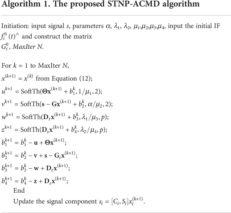
Table 1 The proposed STNP-ACMD algorithm.

According to the formulation of the frequency increment of the demodulated signals (Hou and Shi, 2013) calculated in Equation (14), we have,

$\begin{array}{ll}{s}_i=G_i{x}_i=[C_i,S_i]x_i& (15)\end{array}$

It should be noted that Algorithm 1 is only used for estimating the first signal component. To estimate other components gradually, like traditional signal decomposition methods such as empirical mode decomposition (EMD) and variational mode decomposition (VMD), the first component denoted by $\stackrel{\wedge }{s_1(t)}$ is removed from the original observation signal, that is,

$\begin{array}{ll}{R}_1(t)=s(t)-\stackrel{\wedge }{s_1(t)}& (16)\end{array}$

where R₁(t) denotes the residual signal after removing the first estimated signal from the original observation. Then, the R₁(t) is treated as a new original signal, same procedures in Algorithm 1 will be repeated for extracting the second estimated signal $\stackrel{\wedge }{s_2(t)}$, by parity of reasoning, until the residual signal meets the pre-determined threshold, such as $\rho =\Delta s^j(t)={║s_i^j(t)-s_i^{j-1}(t)║}_2^2/{║s(t)║}_2^2,0<i,j\le K$. Hence, the original observation signal s(t) can be expressed as,

$\begin{array}{ll}s(t)={\displaystyle \sum _{i=1}^K\stackrel{\wedge }{s_1(t)}}+R_K(t)& (17)\end{array}$

where R_K (t) is the residual component or additional noise. As a result, the instantaneous frequency (IF) is determined by differentiation $f(t)=\frac{1}{2\pi }\frac{d\psi (t)}{dt}$, and the increment of the IF is calculated as,

$\begin{array}{ll}\stackrel{\wedge }{\Delta f_i(t)}=-\frac{1}{2\pi }\frac{d}{dt}\left(\arctan \left[\frac{b_i^{n+1}(t)}{a_i^{n+1}(t)}\right]\right)=-\frac{1}{2\pi }\frac{a_i^{n+1}(b_i^{n+1})\text{'}-b_i^{n+1}(a_i^{n+1})\text{'}}{{(a_i^{n+1})}^2+{(b_i^{n+1})}^2}& (18)\end{array}$

Motivated by the approach in Ref (Mcneill, 2016)., the final IF can be updated as,

$\begin{array}{ll}{f}_i^{n+1}(t)=f_i^n(t)+{({\mathit{Q}}^{(2)}/\zeta +\mathit{I})}^{-1}\Delta \stackrel{\wedge }{f_i^n(t)}& (19)\end{array}$

where Q^(N)=(Ω^(N))^TΩ^(N), I is an identity matrix, Ω is a second-order derivative operator, ζ is small positive value.

3 Numerical simulation

A numerical simulation case is conducted to investigate the effectiveness of the proposed approach in terms of the accuracy and robustness versus the traditional ACMD (Chen et al., 2019), the VNCMD method (Chen et al., 2017), the EEMD method (Wu and Huang, 2009), and the VMD method (Dragomiretskiy and Zosso, 2014). A simulated signal that is corrupted by ambient noise is constructed as follows,

$\begin{array}{ll}\{\begin{array}{l}x(t)=x_1(t)+x_2(t)+x_3(t)+x_4(t)+x_5(t)+x_6(t)\\ x_1(t)=Q_1(1+A{M}_1)\exp (-0.05t)\cos \left[2\pi (2+200t-50t^2-2t^3-5t^4)\right]\\ x_2(t)=0.2Q_2(1+A{M}_2)\exp (-0.08t)\cos \left[2\pi (4+80t+20t^2-1.6t^3+0.15t^4)\right]\\ x_3(t)=0.8\exp (-0.08t)\cos \left[2\pi (5+140t+20t^2-2t^3+0.2t^4)\right]\\ x_4(t)=0.5\exp (-0.2t)\cos \left[2\pi (3+20t+40t^2-1.5t^3+0.4t^4)\right]\\ x_5(t)=heavytailednoise\\ x_6(t)=sigma\times \text{randn}(1,N)\end{array}& (20)\end{array}$

where the varying speed profiles are Q₁=0.1(1+2t)²+1, Q₂=0.12(1+2t)²+2 ,the amplitude profiles are $A{M}_1=0.3\sin ({\displaystyle \underset{0}{\overset{t}{\int }}2\pi (1+2t)}dt)$, $A{M}_2=0.3\sin (2{\displaystyle \underset{0}{\overset{t}{\int }}2\pi (1+2t)}dt)$, N = 512 is the number of sampling points, the sampling frequency f_s = 512 Hz, and the sampling time is 1 s.

The simulated synthetic signal consists of five parts, both x₁(t) and x₂(t) are amplitude modulation frequency modulation (AM–FM) signals, x₃(t) is a frequency modulation (FM) signal, x₄(t) is an additive Gaussian white noise (GWN) with standard deviation sigma = 1, and x₅(t) is a heavy tailed noise (HTN). Both GWN and HTN noises are independent with each other. Of particular interest to us is the mode or signal with small amplitude and heavy tail distribution, which is difficult to identify. Therefore, the addition of HTN noise is to create difficulty in signal estimation, artificially. The HTN is expressed with a symmetric alpha-stable (SαS) distribution with parameter α≠1 and 1< α<2, the expression of SαS distribution is defined as (Kuruoglu et al., 1998; Liu et al., 2022),

$\begin{array}{ll}{x}_5(t)=S_{\alpha ,\rho }\times \left\{\frac{\sin (\alpha (v+B_{\alpha ,\rho }))}{{(\cos v)}^{1/\alpha }}{(\frac{\cos (v-\alpha (v+B_{\alpha ,\rho }))}{W})}^{(1-\alpha )/\alpha }\right\}& (21)\end{array}$

where W is the exponential random variable, i.e., W~exprnd(N) , random variable v∈(−π/2,π/2) , $B_{\alpha ,\rho }=\frac{\arctan (\rho \tan \frac{\pi \alpha }{2})}{\alpha }$, $S_{\alpha ,\rho }={[1+{\rho }^2{\tan }^2\frac{\pi \alpha }{2}]}^{1/(2\alpha )}$. If the α = 1, the THN can be given as,

$\begin{array}{ll}{x}_5(t)=\frac{2}{\pi }\left[(\frac{\pi }{2}+\rho v)\tan v-\rho \log (\frac{W\cos v}{\frac{\pi }{2}+\rho v})\right]& (22)\end{array}$

The simulated signal is depicted in Figure 1A, where the AM–FM signals x₁(t) and x₂(t), the FM signal x₃(t), the HTN component with parameters α = 1.4, ρ = 1.2 and raw synthetic signal are shown in Figure 1A from top to the bottom, respectively. It can be seen that the AM–FM and FM signals are submerged in the additional noises. The short time Fourier transform (STFT) of the simulated synthetic signal is shown in Figure 1B, it can be seen that the modulation frequencies are fuzzy and disorder and the frequency variation trends could not be detected at all in the STFT diagram.

FIGURE 1

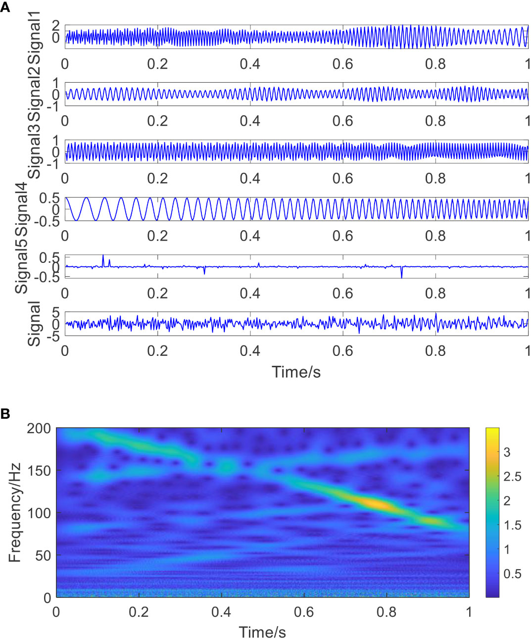
Figure 1 The simulated signal and its STFT diagram. (A) The simulated signal: from top to bottom are signal x₁(t), x₂(t), x₃(t), x₄(t), heavy tailed noise x₅(t) and synthetic signal x(t); (B) the STFT diagram of the simulated synthetic signal.

The proposed STNP-ACMD algorithm is utilized to decompose the simulated synthetic signal. Herein, the model parameters are set as follows: α = 10⁻⁸, ζ = 10⁻⁹, λ₁ = λ₂ = 0.01α, μ₁ = μ₂ = μ₃ = μ₄ = 0.01, and the threshold of signal energy is set to be 0.1. The fractional order of the simulated synthetic signal is 0.0508 using the R/S method (Hurst, 1951; Mason, 2016). The fitted regression lines of the Hurst exponent are shown in Figure 2. Note that the Hurst index of the simulated synthetic signal is a random variable and fluctuated around a value of 0.5 due to the interference from the GWN and HTN noises. By iterating, the signal energies of the first five components are 1.0854, 0.2945, 0.1054, 0.1340, and 0.0459. Thus, four estimated signal components are shown in Figure 3, since the signal energy of the last component is 0.0459<0.1. It can be observed that four estimated signal components match the theoretical signals very well. For the most part, the instantaneous frequencies of the estimated components are basically consistent with the original (or true) ones, which shows the availability of the proposed approach with respect to noise perturbation.

FIGURE 2

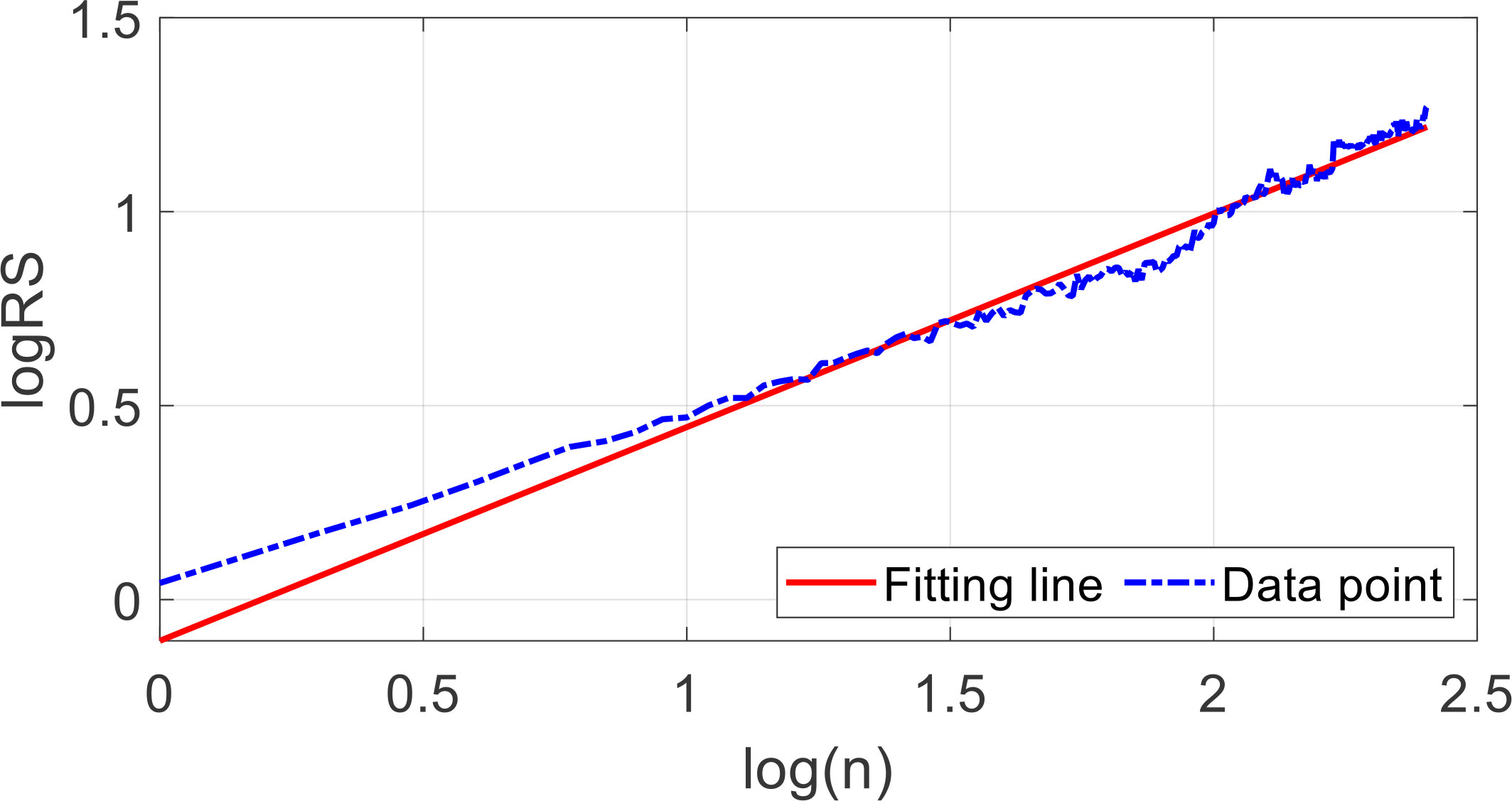
Figure 2 The fitted regression lines of the Hurst exponent.

FIGURE 3

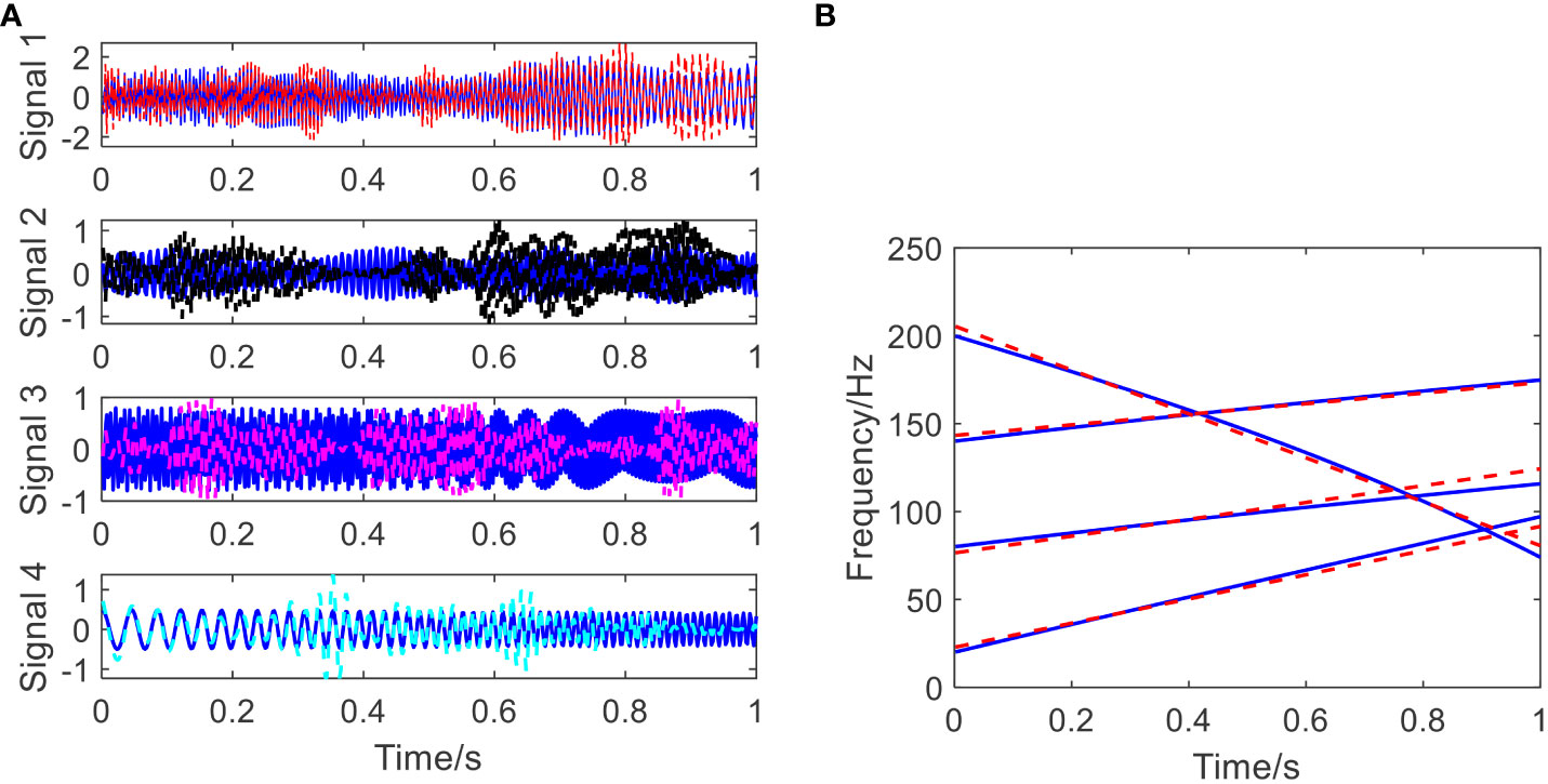
Figure 3 The estimated signal components and estimated time frequency plot using the proposed approach. (A) The estimated components (blue: true; red, black, carmine, and cyan: estimated ones); (B) The estimated time frequency plot (blue: true; red: estimated).

For comparison, the ACMD method (Chen et al., 2019), the VNCMD method (Chen et al., 2017), the EEMD method (Wu and Huang, 2009), and the VMD method (Dragomiretskiy and Zosso, 2014) are employed for decomposing the simulated signal. The estimated components generated via the ACMD and the VNCMD algorithms are displayed in Figures 4A, 5A, and the IFs of the estimated components generated via the ACMD and the VNCMD methods are shown in Figures 4B, 5B. Herein, the number of sub-components is considered and set to be four in the ACMD and VNCMD methods. It can be seen from Figure 4A that the ACMD and the VNCMD methods can slightly extract the components as the proposed does. However, the IFs of the estimated components are mussy and intricate, In the meantime, many wrong IFs are estimated from the ACMD and the VNCMD methods, as shown in Figures 4B, 5B. The main reason behind this shortcoming is that the spatio-temporal coupled information and physical cross-knowledge are not considered by the ACMD and the VNCMD methods, which is also the main limitation of the ACMD and the VNCMD methods in practical applications. It can be concluded that the cross-knowledge or coupled information of the IFs of four pre-estimated components can be demodulated or isolated by the proposed approach, but the ACMD and the VNCMD methods failed.

FIGURE 4

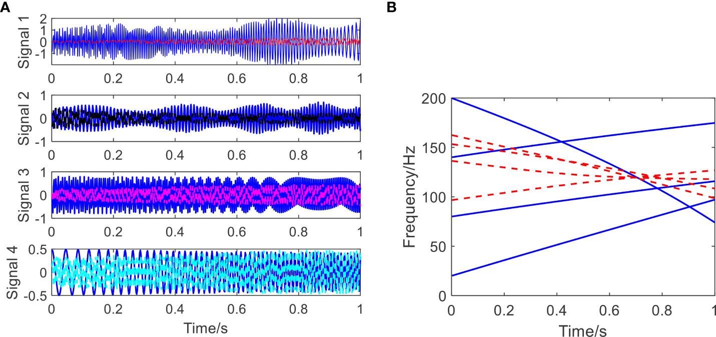
Figure 4 The estimated signal components and estimated time frequency plot using the ACMD method. (A) The estimated components (blue: true; red, black, carmine and cyan: estimated ones); (B) the estimated time frequency plot (blue: true; red: estimated).

FIGURE 5

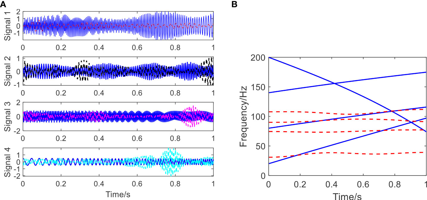
Figure 5 The estimated signal components and estimated time frequency plot using the VNCMD method. (A) The estimated components (blue: true; red, black, carmine and cyan: estimated ones); (B) the estimated time frequency plot (blue: true; red: estimated).

Additionally, the estimated components generated via the EEMD and the VMD methods are displayed in Figures 6A, C, and the instantaneous frequencies of the estimated components generated via the EEMD and the VMD methods are shown in Figures 6B, D, respectively. As shown in Figure 6, many spurious IMF components without physical meaning are separated, and the Hilbert Huang Transform (HHT) cannot reveal the actual IF patterns of the estimated components, as shown in Figures 6B, D, which means the EEMD and the VMD methods still suffer from severe issues with the HHT, i.e., models aliasing. The comparison results reveal that the hidden components containing crossover frequencies can be separated and estimated one by one using the proposed STNP-ACMD algorithm. The crossover IFs are much closer approximations to the real ones.

FIGURE 6

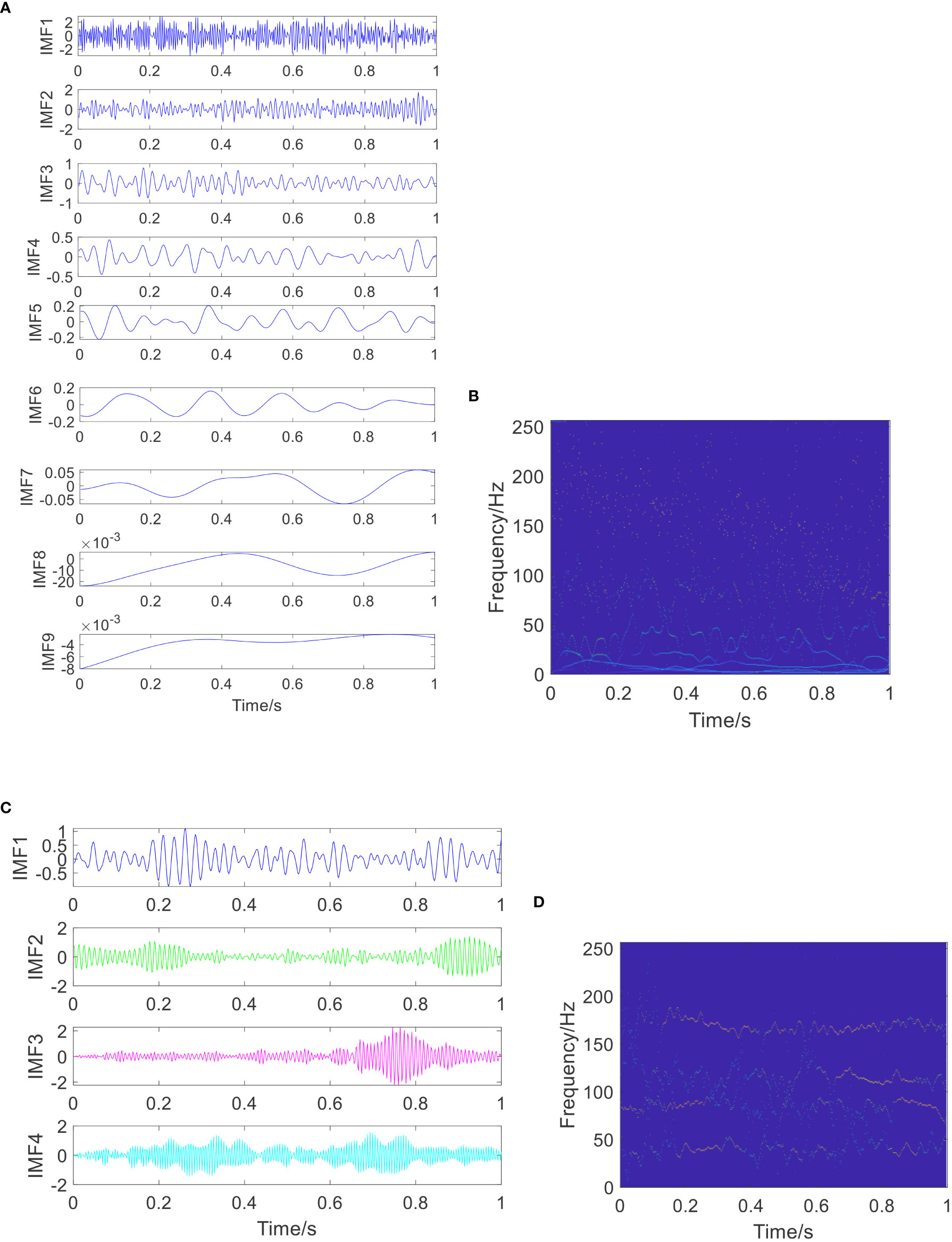
Figure 6 The estimated signal components and their estimated time-frequency plots using the EEMD and the VMD methods. (A) The estimated components using the EEMD method; (B) the estimated time–frequency plot of the estimated components using the EEMD method; (C) the estimated components using the VMD method; and (D) the estimated time-frequency plot of the estimated components using the VMD method.

4 Experimental case of real-world applications

The simulated case in Section 3 indicates that the proposed STNP-ACMD algorithm has promising advantages in analyzing simulated signals with crossover instantaneous frequencies. Therefore, in this section, the proposed STNP-ACMD algorithm will be used to extract the signal components and their crossover IFs from seafloor dynamic data and further achieve the exploration of the tidal law and magnetotelluric dynamic analysis in deep seafloor.

4.1 Introduction of experimental datasets

The experimental datasets of seafloor dynamic data are provided by the Institute of Acoustics, Chinese Academy of Sciences (Chang et al., 2019). The diagram of the deep seafloor observation network system in the South China Sea and the observation position of the submarine dynamic platform (represented by the red flag, with 111.0675°E and 17.5811°N) are shown in Figures 7A, B. In this experiment, the acoustic Doppler current profilers (ADCP) of type Teledyne were used for collecting the observation elements including seafloor temperature, seafloor water salinity, seafloor water flow rate #1, seafloor water flow rate #2, seafloor water flow rate #3, seafloor water flow rate #4, roll data, bow data, and tilt data. Those datasets were processed with the following operations: autocompletion of default value, verification of data threshold interval, etc.

FIGURE 7

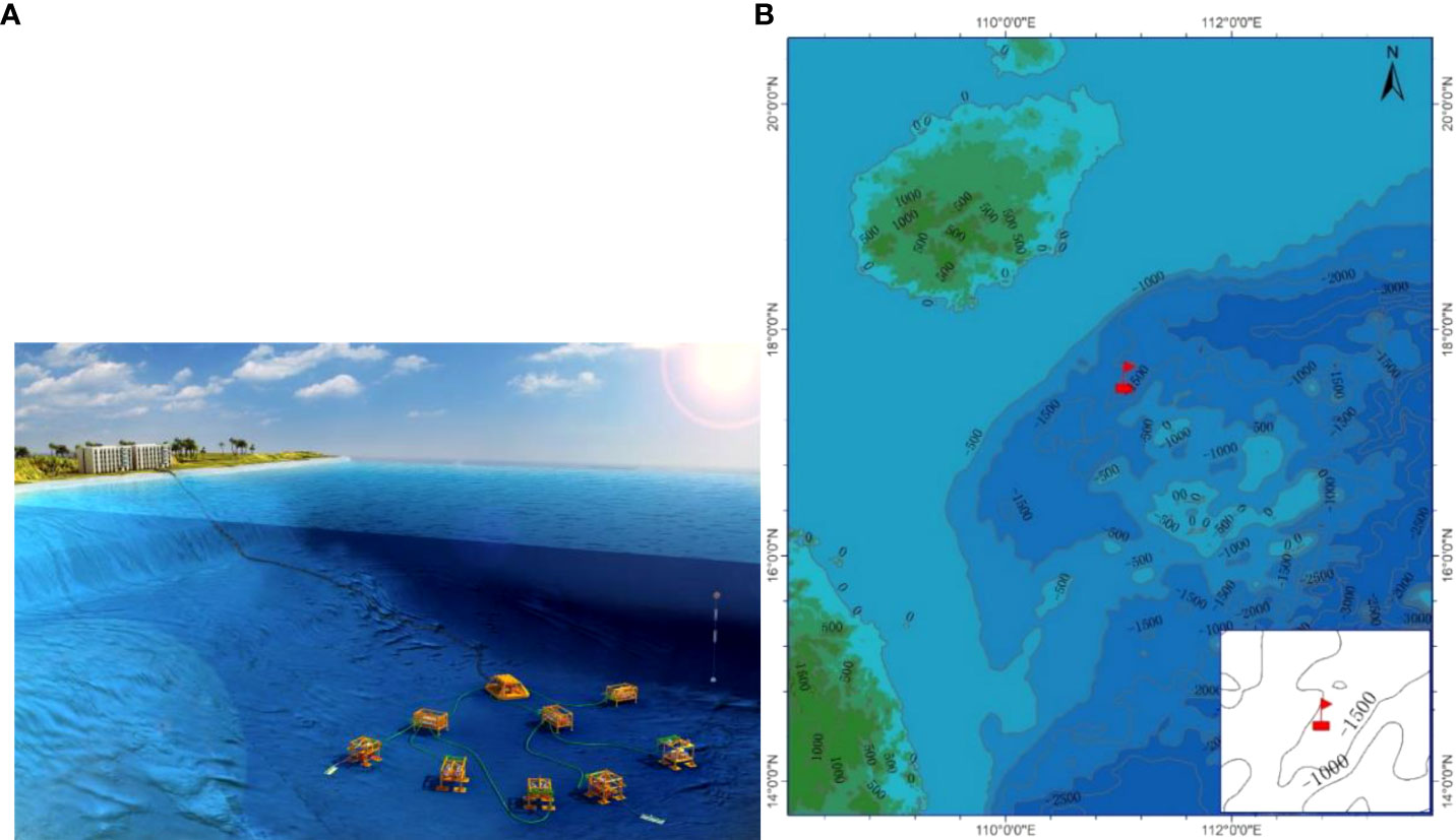
Figure 7 The deep seafloor observation network system and observation position (Chang et al., 2019). (A) The diagram of the deep seafloor observation network system in the South China Sea; (B) the observation position of submarine dynamic platform (represented by red flag).

4.2 Results analysis

In this work, the seafloor water flow rates #1 with 2,048 points are employed. The operating frequency of ADCP was 150 kHz. The number of observation layers was 30, each layer was 4 m, and sampling was conducted at an interval of 10 min (Chang et al., 2019). The raw signal waveform and its time frequency diagram of seafloor water flow rates #1 with 2,048 points are shown in Figure 8. It can be seen from Figure 8A that high frequency vibration components are accompanied by a slowly decreasing low frequency trend component, and the frequency information of 2,048 points is mainly concentrated in the low-frequency band. No obvious instantaneous frequency trends can be found to track the variation of the velocity in the deep seafloor, as shown in Figure 8B.

FIGURE 8

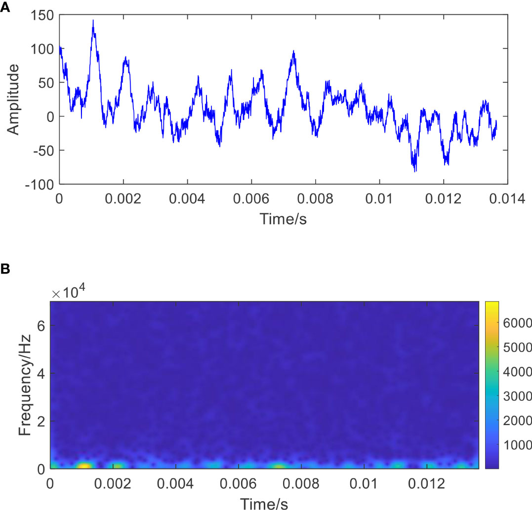
Figure 8 Ocean water velocity and its time frequency diagram. (A) Ocean water velocity of deep seabed collected by acoustic Doppler current-meter sensor; (B) the time frequency diagram of ocean water velocity.

The proposed STNP-ACMD algorithm is applied to estimate the sub-components and their IFs, where the threshold of signal energy is set to be 0.03. Due to the disturbance of fluctuating trends, detrended and normalization operations were performed on the raw seafloor water flow rates #1 with 2,048 points, and then the fractional order of the simulated synthetic signal is 0.3182 using the R/S method (Hurst, 1951; Mason, 2016). The fitted regression lines of the Hurst exponent are shown in Figure 9, and the signal energies of the first six components and the residual are summarized in Table 2. Therefore, the first six estimated components are selected and presented in Figure 10. It can be found that the waveform pattern and fluctuating trend of signal 1 are the same as the raw seafloor water flow rates (see Figure 8A). Meanwhile, as demonstrated in Table 2, five high-frequency components, i.e., from signals 2 to 6, with lower energy are also extracted and thus contain more valuable information with respect to interference from other factors such as fauna and plankton. The TF diagram of the estimated components using the proposed approach is shown in Figure 11. It shows that the crossover instantaneous frequencies between signals 1 and 2 can be extracted clearly. Those features above indicate that the patterns of low-frequency trend and high-frequency fluctuation of the raw seafloor water flow rate can be captured and accurately estimated using the proposed approach.

FIGURE 9

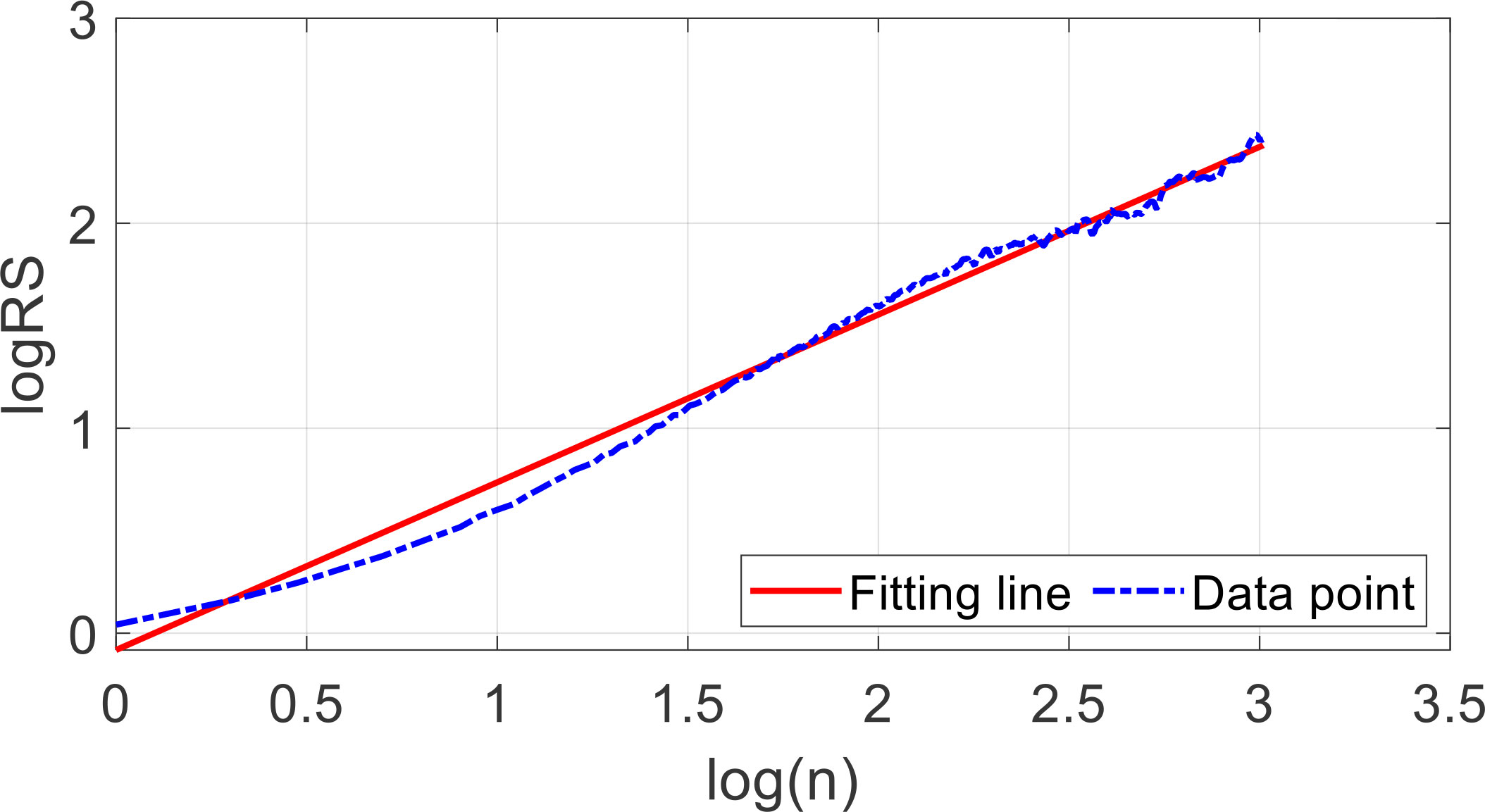
Figure 9 The fitted regression lines of the Hurst exponent.

TABLE 2

Table 2 The signal energy of each estimated component.

FIGURE 10

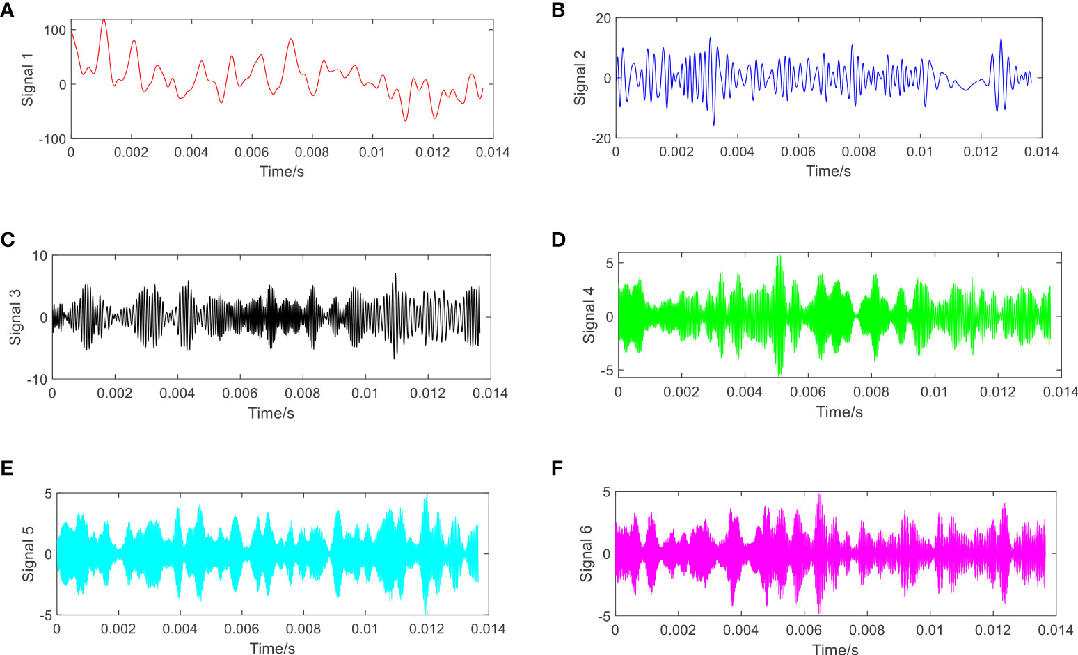
Figure 10 The decomposed signal components using the proposed approach. (A) Component 1; (B) component 2; (C) component 3; (D) component 4; (E) component 5; and (F) component 6.

FIGURE 11

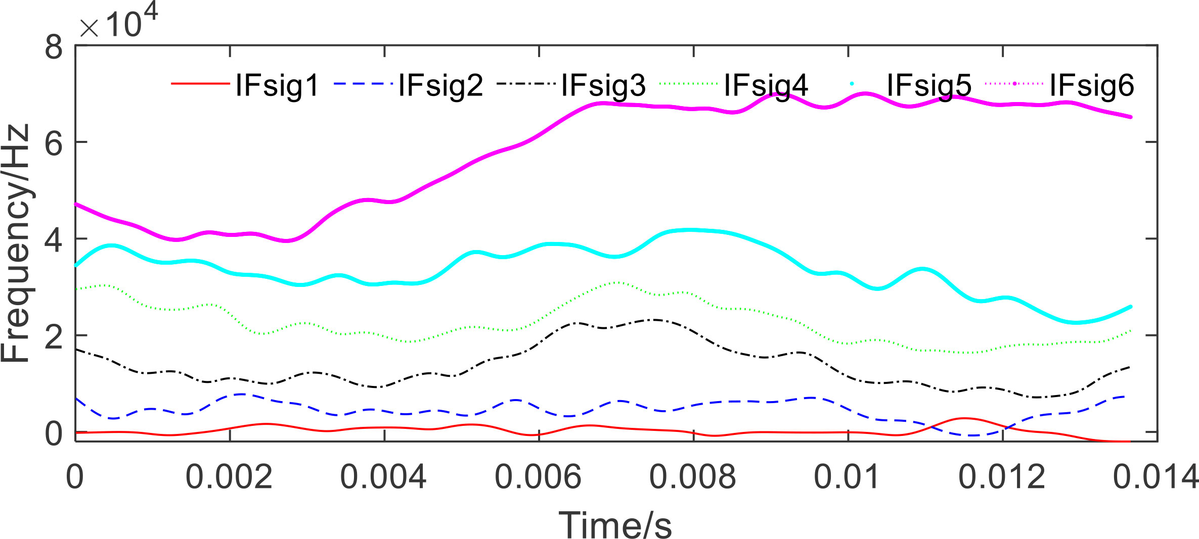
Figure 11 The TF diagram of the estimated components using the proposed approach.

To investigate the superiority of the proposed approach, four benchmarks, including the ACMD method (Chen et al., 2019), the VNCMD method (Chen et al., 2017), the EEMD method (Wu and Huang, 2009), and the VMD method (Dragomiretskiy and Zosso, 2014), are introduced for comparisons. The estimated components generated via the ACMD and the VNCMD methods are displayed in Figures 12, 14A, and the IFs of the estimated components generated via the ACMD and the VNCMD methods are shown in Figures 13, 14B. Herein, the number of the decomposed components is determined to be 6 in the ACMD and the VNCMD methods, according to the proposed approach. As shown in Figure 12, it shows that the waveform of signal 1, estimated using the ACMD method, is slightly coincident with that of raw seafloor water flow rate, but the other five components still belong to low-frequency components (see Figures 12B–F), and all of the IFs are aliased together, simultaneously. As shown in Figure 14, the whole estimated components that are generated from the VNCMD method are similar to the waveform of the original signal, and the frequency characteristics of the other components cannot be revealed at all. In addition, the same to the results of the ACMD method, all of the instantaneous frequencies are aliased together, simultaneously. That is to say, the high-frequency information of the raw signal is not captured using the ACMD and the VNCMD methods, which is contrary to the characteristics of the raw signal.

FIGURE 12

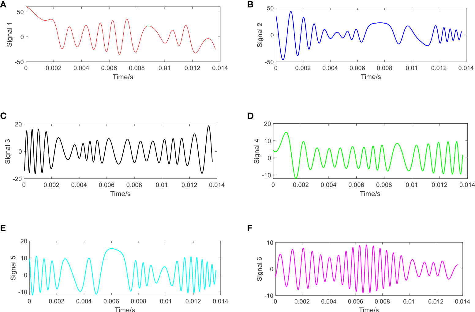
Figure 12 The estimated components using the ACMD method. (A) Component 1; (B) component 2; (C) component 3; (D) component 4; (E) component 5; and (F) component 6.

FIGURE 13

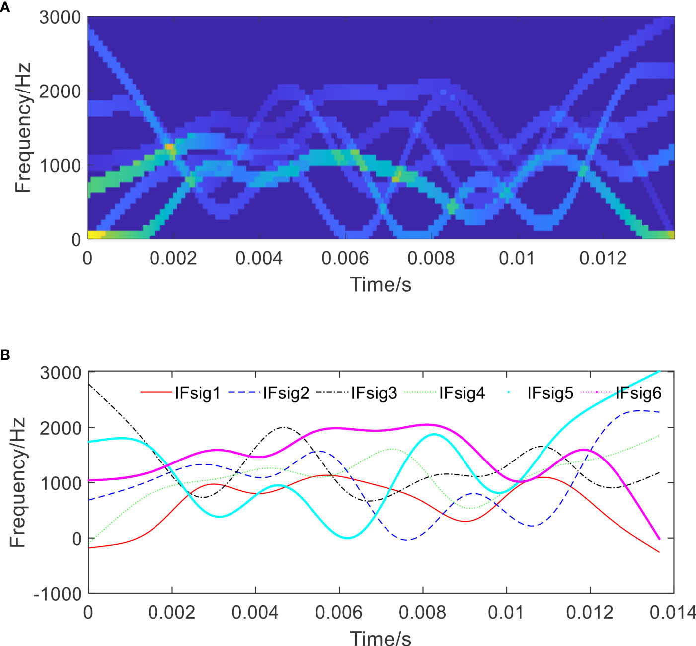
Figure 13 The TF diagram and IF plot of the estimated components using the ACMD method. (A) The TF diagram of the estimated components; and (B) the IF plot of the estimated components.

FIGURE 14

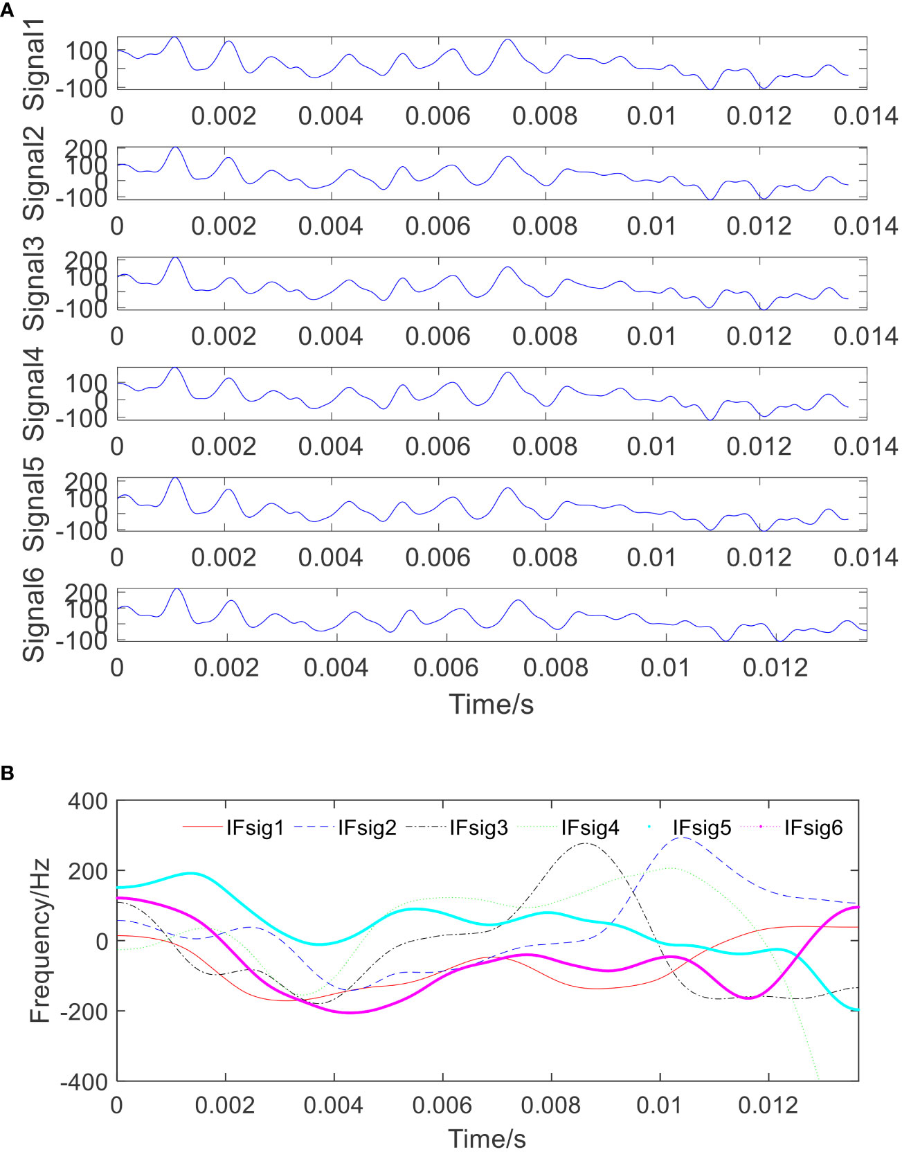
Figure 14 The estimated signal components and their estimated time-frequency plots using the VNCMD method. (A) The estimated components using the VNCMD method; and (B) the estimated time-frequency plot of the estimated components using the VNCMD method.

In addition, the estimated components and their IFs generated via the EEMD and VMD methods are shown in Figure 15. It shows that the sub-components can be extracted and decomposed through the EEMD and VMD methods from the high frequency to the low frequency. Obviously, the waveform trend of the low frequency cannot also be captured by the EEMD and VMD methods because the wideband modes are still overlapping in the frequency domain. Meanwhile, the modes exhibit poor energy concentration in time–frequency representations and also present a poor correlation with the raw signal of seafloor water flow rates. Therefore, it can be concluded that the EEMD and VMD methods cannot reveal the time-frequency pattern of the signal with crossing regions, and the proposed method can achieve more reliable estimated results and clear fluctuating patterns of the IFs in real-world applications.

FIGURE 15

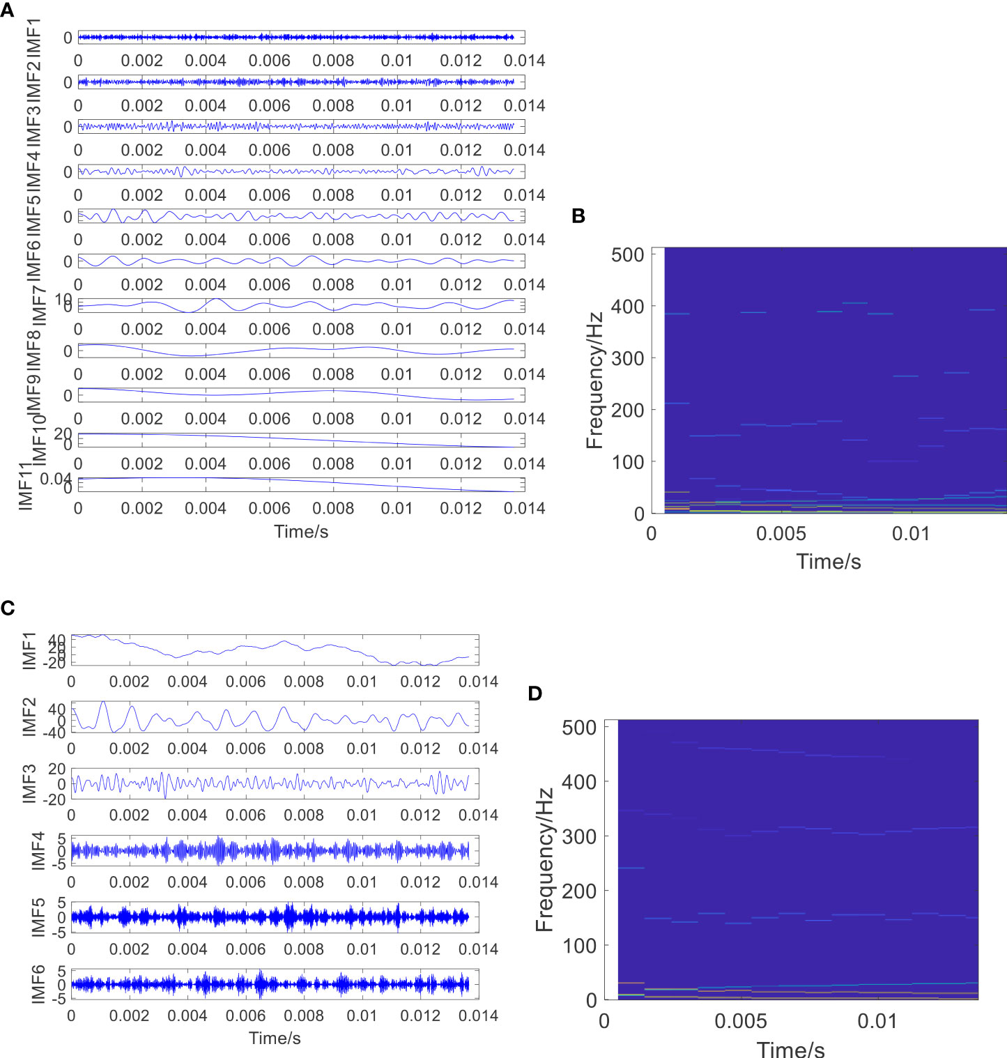
Figure 15 The estimated signal components and their estimated time–frequency plots using the EEMD and VMD methods. (A) The estimated components using the EEMD method; (B) the estimated time–frequency plot of the estimated components using the EEMD method; (C) the estimated components using the VMD method; and (D) the estimated time–frequency plot of the estimated components using the VMD method.

5 Conclusions

In this paper, a novel spatio-temporal nonconvex penalty adaptive chirp mode decomposition (STNP-ACMD) algorithm is proposed for recompositing the complicated multi-component whose mono-modes have crossed IFs or overlapped frequency information. The spatio-temporal relationship among estimated components is considered via incorporating a nonconvex penalty term into the cost function in terms of a temporal matrix and a spatial matrix. The rationale for exploiting the coupled nature of the available information within the estimated components is given in detail. Meanwhile, the cost function can be effectively solved by the split Bregman algorithm, and the characteristics of the fractional-order of the multi-component are also considered. The results of synthetic simulated cases and specific experimental cases are introduced between the proposed approach and the state-of-the-art benchmarks and indicate that the proposed STNP-ACMD has higher decomposed accuracy and superiority in component estimation and IFs in terms of crossed IFs scenarios.

However, it should be highlighted that due to the fact that the real IF information is unknown, the estimated time–frequency ridge cannot be verified in practical application of seafloor dynamic engineering. The STNP-ACMD method proposed in this work is a deliberate attempt and a promising exploration. In addition, one of the disadvantages in the work focuses on parameter setting. Arbitrary parameter settings are taken in this work, which lacks robustness for time-varying scenarios. Therefore, future investigation will be devoted to enhancing the robustness of the proposed method, including parameter optimization and noise detection, and the multi-dimensional and complicated time-varying scenarios in industrial areas and ocean engineering applications will also be explored.

Data availability statement

The original contributions presented in the study are included in the article/supplementary material. Further inquiries can be directed to the corresponding author.

Author contributions

The author confirms being the sole contributor of this work and has approved it for publication.

Funding

This work is supported by the National Natural Science Foundation of China (No. 52205079), the Foundation of High-level Talents (No. RC412104), the Natural Science Research Project of Universities in Anhui Province (No. KJ2021A0155), and the State Key Laboratory of Mechanical System and Vibration (No. MSV202015). The insightful comments and profound suggestions from reviewers are greatly appreciated.

Conflict of interest

The author declares that the research was conducted in the absence of any commercial or financial relationships that could be construed as a potential conflict of interest.

Publisher’s note

All claims expressed in this article are solely those of the authors and do not necessarily represent those of their affiliated organizations, or those of the publisher, the editors and the reviewers. Any product that may be evaluated in this article, or claim that may be made by its manufacturer, is not guaranteed or endorsed by the publisher.

References

Auger F., Flandrin P., Lin Y. T., McLaughlin S., Meignen S., Oberlin T., et al. (2013). Time-frequency reassignment and synchrosqueezing: an overview. IEEE Signal Process Mag. 30 (6), 32–41. doi: 10.1109/MSP.2013.2265316

CrossRef Full Text | Google Scholar

Chang Y. G., Zhang F., Guo Y. G., Song X. Y., Yang J., Liu R. Y. (2019). The ocean dynamic datasets of seafloor observation network experiment system at the south China sea. China Sci. Data 4 (4):48-55. doi: 10.11922/sciencedb.823

CrossRef Full Text | Google Scholar

Chen Q. M., Chen J. H., Lang X., Xie L., Lu S., Su H. Y. (2020). Detection and diagnosis of oscillations in process control by fast adaptive chirp mode decomposition. Control Eng. Pract. 97, 104307. doi: 10.1016/j.conengprac.2020.104307

CrossRef Full Text | Google Scholar

Chen S. Q., Dong X. J., Peng Z. K., Zhang W. M., Meng G. (2017). Nonlinear chirp mode decomposition: A variational method. IEEE T. Signal Process. 65 (22), 6024–6037. doi: 10.1109/TSP.2017.2731300

CrossRef Full Text | Google Scholar

Chen S. Q., Yang Y., Peng Z. K., Dong X. J., Zhang W. M., Meng G. (2019). Adaptive chirp mode pursuit: algorithm and applications. Mech. Syst. Signal Process. 116, 566–584. doi: 10.1016/j.ymssp.2018.06.052

CrossRef Full Text | Google Scholar

Chen S. Q., Yang Y., Peng Z. K., Wang S. B., Zhang W. M., Chen X. F. (2019). Detection of rub-impact fault for rotor-stator systems: a novel method based on adaptive chirp mode decomposition. J. Sound Vib. 440, 83–99. doi: 10.1016/j.jsv.2018.10.010

CrossRef Full Text | Google Scholar

Chen K., Zhao Q. X., Deng M., Luo X. H., Jing J. E. (2020). Seawater motion-induced electromagnetic noise reduction in marine magnetotelluric data using current meters. Earth Planets Space 72, (4). doi: 10.1186/s40623-019-1129-0

CrossRef Full Text | Google Scholar

Clausel M., Oberlin T., Perrier V. (2015). The monogenic synchrosqueezed wavelet transform: a tool for the decomposition/demodulation of AM-FM images. Appl. Comput. Harmon. Anal. 39, 450–486. doi: 10.1016/j.acha.2014.10.003

CrossRef Full Text | Google Scholar

Corsaro S., Simone V. D., Marino Z. (2021). Split bregman iteration for multi-period mean variance portfolio optimization. Appl. Math. Comput. 392, 125715. doi: 10.1016/j.amc.2020.125715

PubMed Abstract | CrossRef Full Text | Google Scholar

Daubechies I., Lu J. F., Wu H. T. (2011). Synchrosqueezed wavelet transforms: An empirical mode decomposition-like tool. Appl. Comput. Harmon. A 30 (2), 243–261. doi: 10.1016/j.acha.2010.08.002

CrossRef Full Text | Google Scholar

Dong H. R., Yu G., Li Y. Y. (2022). Theoretical analysis and comparison of transient-extracting transform and time-reassigned synchrosqueezing transform. Mech. Syst. Signal Process. 178, 109190. doi: 10.1016/j.ymssp.2022.109190

CrossRef Full Text | Google Scholar

Dragomiretskiy K., Zosso D. (2014). Variational mode decomposition. IEEE T. Signal Process 62 (3), 531–544. doi: 10.1109/TSP.2013.2288675

CrossRef Full Text | Google Scholar

Gilles J. (2013). Empirical wavelet transform. IEEE T. Signal Process. 61 (16), 3999–4010. doi: 10.1109/TSP.2013.2265222

CrossRef Full Text | Google Scholar

Goldstein T., Osher S. (2009). The split bregman method for L1 regularized problems. SIAM J. Imag. Sci. 2, 323–343. doi: 10.1137/080725891

CrossRef Full Text | Google Scholar

Hou T. Y., Shi Z. (2013). Data-driven time frequency analysis. Appl. Comput. Harmon. Anal. 35 (2), 284–308. doi: 10.1016/j.acha.2012.10.001

CrossRef Full Text | Google Scholar

Huang N. E., Shen Z., Long S. R., Wu M. C., Shih H. H., Zheng Q., et al. (1998). The empirical mode decomposition and the Hilbert spectrum for nonlinear and non-stationary time series analysis. Proc. R. Soc. A: Mathematical Phys. Eng. Sci. 454,1971 903–995. doi: 10.1098/rspa.1998.0193

CrossRef Full Text | Google Scholar

Hurst H. E. (1951). Long-term storage capacity reservoirs. Trans. Am. Soc Civil Eng. 116, 770–808. doi: 10.1061/TACEAT.0006518

CrossRef Full Text | Google Scholar

Jiang Y., Liu S. Y., Zhao N., Xin J. Z., Wu B. (2020). Short-term wind speed prediction using time varying filter-based empirical mode decomposition and group method of data handling-based hybrid model. Energ. Convers. Manage. 220, 113076. doi: 10.1016/j.enconman.2020.113076

CrossRef Full Text | Google Scholar

Kuruoglu E. E., Fitzgerald W. J., Rayner P. J. W. (1998). Near optimal detection of signals in impulsive noise modeled with a symmetric /spl alpha/-stable distribution. IEEE Commun. Lett. 2 (10), 282–284. doi: 10.1109/4234.725224

CrossRef Full Text | Google Scholar

Li R., Chen H., Fang Y. X., Hu Y., Chen X. P., Li J. (2022). Synchrosqueezing polynomial chirplet transform and its application in tight sandstone gas reservoir identification. IEEE Geosci. Remote S., 19:1–5. doi: 10.1109/LGRS.2021.3071318

CrossRef Full Text | Google Scholar

Lin Y., Lin Z. X., Liao Y., Li Y. Z., Xu J. L., Yan Y. (2022). Forecasting the realized volatility of stock price index: A hybrid model integrating CEEMDAN and LSTM. Expert Syst. Appl. 206, 117736. doi: 10.1016/j.eswa.2022.117736

CrossRef Full Text | Google Scholar

Liu X., Du L., Xu S. (2022). GLRT-based coherent detection in sub-Gaussian symmetric alpha-stable clutter. IEEE Geosci. Remote S. 19 1-5, 8015405. doi: 10.1109/LGRS.2021.3094847

CrossRef Full Text | Google Scholar

Li L., Yu X. R., Jiang Q. T., Zang B., Jiang L. (2022). Synchrosqueezing transform meets α-stable distribution: An adaptive fractional lower-order SST for instantaneous frequency estimation and non-stationary signal recovery. Signal Process. 201, 108683. doi: 10.1016/j.sigpro.2022.108683

CrossRef Full Text | Google Scholar

MacLennan K., Li Y. G. (2013). Denoising multicomponent CSEM data with equivalent source processing techniques. Geophysics 78 (3), 125–135. doi: 10.1190/geo2012-0226.1

CrossRef Full Text | Google Scholar

Majumdar A., Ward R. K. (2012). On the choice of compressed sensing priors and sparsifying transforms for MR image reconstruction: An experimental study. Signal Process. Image Commun. 27 (9), 1035–1048. doi: 10.1016/j.image.2012.08.002

CrossRef Full Text | Google Scholar

Mason D. M. (2016). The Hurst phenomenon and the rescaled range statistic. Stoch. Proc. Appl. 126, (12) 3790–3807. doi: 10.1016/j.spa.2016.04.008

CrossRef Full Text | Google Scholar

Mcneill S. I. (2016). Decomposing a signal into short-time narrow-banded modes. J. Sound Vib. 373, 325e339. doi: 10.1016/j.jsv.2016.03.015

CrossRef Full Text | Google Scholar

Meignen S., Pham D. H., Colominas M. A. (2021). On the use of short-time fourier transform and synchrosqueezing-based demodulation for the retrieval of the modes of multicomponent signals. Signal Process. 178, 107760. doi: 10.1016/j.sigpro.2020.107760

CrossRef Full Text | Google Scholar

Nyqvist D., Durif C., Johnsen M. G., Jong K. D., Forland T. N., Sivle L. D. (2020). Electric and magnetic senses in marine animals, and potential behavioral effects of electromagnetic surveys. Mar. Environ. Res. 155, 104888. doi: 10.1016/j.marenvres.2020.104888

PubMed Abstract | CrossRef Full Text | Google Scholar

Park D., Kwak K., Kim J., Li J. H., Chung W. K. (2019). Underwater localization using received signal strength of electromagnetic wave with obstacle penetration effects. IFAC-Papers Online 52 (21), 372–377. doi: 10.1016/j.ifacol.2019.12.335

CrossRef Full Text | Google Scholar

Schwalenberg K., Gehrmann R. A. S., Bialas J., Rippe D. (2020). Analysis of marine controlled source electromagnetic data for the assessment of gas hydrates in the Danube deep-sea fan, black Sea. Mar. Petrol. Geol.122, 104650. doi: 10.1016/j.marpetgeo.2020.104650

CrossRef Full Text | Google Scholar

Si Y., Kong L. F., Chin J. H., Guo W. C., Wang Q. L. (2022). Whirling detection in deep hole drilling process based on multivariate synchrosqueezing transform of orthogonal dual-channel vibration signals. Mech. Syst. Signal Process. 167, 108621. doi: 10.1016/j.ymssp.2021.108621

CrossRef Full Text | Google Scholar

Tian Y. W., Liu M. Q., Zhang S. L., Zhou T. (2022). Underwater multi-target passive detection based on transient signals using adaptive empirical mode decomposition. Appl. Acoust. 190, 108641. doi: 10.1016/j.apacoust.2022.108641

CrossRef Full Text | Google Scholar

Torres M. E., Colominas M. A., Schlotthauer G., Flandrin P. (2011). “A complete ensemble empirical mode decomposition with adaptive noise,” in IEEE Int. Conf. on Acoust., Speech and Signal Proc. ICASSP, Prague, Czech Republic. 4144–4147 doi: 10.1109/ICASSP.2011.5947265

CrossRef Full Text | Google Scholar

Vashishtha G., Chauhan S., Yadav N., Kumar A., Kumar R. (2022). And tangent entropy in estimation of single-valued neutrosophic cross-entropy for detecting impeller defects in centrifugal pump. Appl. Acoust. 197, 108905. doi: 10.1016/j.apacoust.2022.108905

CrossRef Full Text | Google Scholar

Wu Z., Huang N. (2009). Ensemble empirical mode decomposition: a noise-assisted data analysis method. Adv. Data Sci. Adadp. 1, 1–41. doi: 10.1142/S1793536909000047

CrossRef Full Text | Google Scholar

Zhang P. F., Deng M., Jing J. E., Chen K. (2020). Marine controlled-source electromagnetic method data de-noising based on compressive sensing. J. Appl. Geophys. 177, 104011. doi: 10.1016/j.jappgeo.2020.104011

CrossRef Full Text | Google Scholar

Appendix

For sub-problem P1, the specific derivation process for signal x is given as,

$\begin{array}{ll}\begin{array}{l}F(x)=\arg \underset{x}{\min }{\mu }_1{║u-\Theta x_i-b_1^k║}_2^2+{\mu }_2{║v-s+G_i{x}_i-b_2^k║}_2^2+\\ {\mu }_3{║w-D_t{x}_i-b_3^k║}_2^2+{\mu }_4{║z-D_s{x}_i-b_4^k║}_2^2\\ ={\mu }_1\left[{(u-b_1^k)}^2-2\Theta x_i(u-b_1^k)+{\Theta }^T\Theta x_i^2\right]+\\ {\mu }_2\left[{(v-s-b_2^k)}^2+2G_i{x}_i(v-s-b_2^k)+G_i^T{G}_i{x}_i^2\right]+\\ {\mu }_3\left[{(w-b_3^k)}^2-2D_t{x}_i(w-b_3^k)+D_t^T{D}_t{x}_i^2\right]+\\ {\mu }_4\left[{(z-b_4^k)}^2-2D_s{x}_i(z-b_4^k)+D_s^T{D}_s{x}_i^2\right]\end{array}& \text{(A1)}\end{array}$

$\begin{array}{ll}\begin{array}{l}\frac{\partial F(x)}{\partial x}=-2{\mu }_1\Theta (u-b_1^k)+2{\mu }_1{\Theta }^T\Theta x_i+2{\mu }_2{G}_i(v-s-b_2^k)+2{\mu }_2{G}_i^T{G}_i{x}_i\\ -2{\mu }_3{D}_t(w-b_3^k)+2{\mu }_3{D}_t^T{D}_t{x}_i-2{\mu }_4{D}_s(z-b_4^k)+2{\mu }_4{D}_s^T{D}_s{x}_i\end{array}& \text{(A2)}\end{array}$

Let’s $\frac{\partial F(x)}{\partial x}=0$, that is,

$\begin{array}{ll}\begin{array}{l}2{\mu }_1{\Theta }^T\Theta x_i+2{\mu }_2{G}_i^T{G}_i{x}_i+2{\mu }_3{D}_t^T{D}_t{x}_i+2{\mu }_4{D}_s^T{D}_s{x}_i\\ =2{\mu }_1\Theta (u-b_1^k)-2{\mu }_2{G}_i(v-s-b_2^k)+2{\mu }_3{D}_t(w-b_3^k)+2{\mu }_4{D}_s(z-b_4^k)\end{array}& \text{(A3)}\end{array}$

$\begin{array}{ll}{x}_i=\frac{{\mu }_1\Theta (u-b_1^k)-{\mu }_2{G}_i(v-s-b_2^k)+{\mu }_3{D}_t(w-b_3^k)+{\mu }_4{D}_s(z-b_4^k)}{{\mu }_1{\Theta }^T\Theta +{\mu }_2{G}_i^T{G}_i+{\mu }_3{D}_t^T{D}_t+{\mu }_4{D}_s^T{D}_s}& \text{(A4)}\end{array}$