 Chiara M. Bertelli*
 William G. Bennett
 Harshinie Karunarathna
 Dominic E. Reeve
 Richard K. F. Unsworth
 James C. Bull
- Faculty of Science and Engineering, Swansea University, Swansea, Wales, United Kingdom
Habitat suitability modelling (HSM) is a tool that is increasingly being used to help guide decision making for conservation management. It can also be used to focus efforts of restoration in our oceans. To improve on model performance, the best available environmental data along with species distribution data are needed. Marine habitats tend to have ecological niches defined by physical environmental conditions and of particular importance for shallow water species is wave energy. In this study we examined the relative improvements to HSM outputs that could be achieved by producing high-resolution Delft-3D modelled wave height data to see if model predictions at a fine-scale can be improved. Seagrasses were used as an exemplar and comparisons at fine-scale showed considerable differences in the area predicted suitable for seagrass growth and greatly increased the importance of waves as a predictor variable when compared with open-source low resolution wave energy data.
1. Introduction
There is growing interest in the use of nature-based solutions to help mitigate the worst impacts of climate change. The greatest emphasis around this interest is on the restoration of habitats. With 2021 to 2030 defined as the UN decade of ecosystem restoration the ambition for re-building biodiversity has never been greater. This includes increasing focus on restoration in the ocean (Danovaro et al., 2021) with projects concentrating on restoration of oysters, coral reefs, mangroves, seagrasses and saltmarshes (Waltham et al., 2020).
Conservation research requires long term surveying campaigns over large areas, which needs commitment to a well-funded, strategic programme of measurement. Due to the practical difficulties this poses, there are limited datasets on habitat quality and extent. A consequence to this is that it is very difficult to direct restoration efforts to places where they will have the best chance of success.
Habitat suitability modelling (HSM) is a tool increasingly used to help guide that decision making. Also known as species distribution models (SDM) and ecological niche models (ENM), they all follow the same premise of capturing the realised niche of a species which can be used for different aims (Naimi and Araújo, 2016; Guisan et al., 2017). HSM can be used to predict distributions of rare and/or vulnerable species for the purposes of conservation management (Thompson et al., 2014; Rowden et al., 2017), assessing changes in distributions of key or invasive species from climate change (Valle et al., 2014) and for informing the most suitable area for habitat conservation and restoration (Adams et al., 2016; Hu et al., 2021).
This type of modelling uses environmental parameters that are known to determine or affect the distribution and presence of the species in question and then projects this to predict where that species should be able to exist if these parameters are met (Guisan et al., 2017). To be able to do this successfully, the availability of good species presence or distribution and environmental parameters is needed to be able to provide models with enough data for testing and training (Guisan et al., 2017; Araújo et al., 2019). Environmental parameters will be made up of the conditions that not only limit, but also influence the distribution and range of the species being studied. Accurate habitat presence data is one of the most important factors for successful HSM as inaccuracies in distribution data will lead to constrained models (Araújo et al., 2019). Presence data need to consist of geographical locations of species and therefore point data (coordinates) are often the most useful and easiest to use.
Seagrass meadows provide an excellent case study for understanding the use of HSMs in the marine environment as they are geographically abundant, have a well-defined environmental range within shallow coastal waters, have a growing interest with regard to restoration initiatives, yet remain poorly mapped (McKenzie et al., 2020; Green et al., 2021). In Europe, the field of seagrass restoration, has grown significantly over the last decade as a result of the increased understanding of the extent of degradation to this marine habitat (Gamble et al., 2021). Zostera marina is a meadow forming seagrass species with a wide geographical range across the northern hemisphere, between 27 and 70°N. For Z. marina, as a submerged aquatic vegetation, the parameters that affect its distribution include light availability (Dennison and Alberte, 1985; Bertelli and Unsworth, 2018), water depth (affecting light attenuation) (Nielsen et al., 2002), sea water temperature (Marsh et al., 1986; Moore and Jarvis, 2008), salinity (Salo et al., 2014), and physical factors such as exposure to waves and currents (Fonseca and Bell, 1998; van Katwijk and Hermus, 2000; Koch et al., 2001). Seagrasses are generally known to exist in shallow, sheltered coastal areas, in soft sediments (Koch et al., 2006). Around the UK and Ireland, these locations are predominantly east or north-east facing bays where they are sheltered from prevailing wind directions and wave fetch, or within lagoons and estuaries (D’Avack et al., 2019).
A review of previous seagrass HSM studies (Bertelli et al., 2022) found the most commonly used environmental parameters to be seawater temperature, bathymetry, light availability, salinity, wave action, substrate and seabed slope. However, the variables ultimately used will also be somewhat dependent upon what environmental data is readily available and its temporal and spatial resolution. Light availability, specifically Photosynthetically Active Radiation (PAR) which is the spectral range of light that is used for photosynthesis, is arguably one of the most important variables to consider as this will determine where plants can survive within coastal waters (Lee et al., 2007; Short et al., 2007; Kuusemäe et al., 2016). Bathymetry is also key in determining where seagrass can exist, as light decreases with depth as it is attenuated (Duarte, 1991). Within its geographical range, Z. marina is usually found within a narrow depth range, typically up to 5-10 m deep depending on water clarity (Davison and Hughes, 1998; Nielsen et al., 2002; Krause-Jensen et al., 2003; Lee et al., 2007; Jackson et al., 2013). Z. marina can tolerate a wide temperature range from -1°C in Arctic regions to 30°C in the subtropics. However, temperature will affect respiration rates within plants and will have significant influence on life stages, such as flowering and germination. Z. marina is also tolerant to a range of salinities and can be found within estuaries as well as fully oceanic conditions, from 18 PSU to 40 PSU (D’Avack et al., 2019).
Where light limitation is not an issue, such as in uniformly shallow areas unaffected by other water quality issues, other physical parameters will be more important in influencing seagrass presence. Seagrasses are exposed to localised hydrodynamics in the form of waves, tides, wind driven currents and wave driven currents (Koch et al., 2006) and these physical factors have been recognised as important factors in affecting spatial distribution and the minimum depth of colonisation (Stevens and Lacy, 2012). Water movement is important for seagrass growth, but where hydrodynamic energy is too high it can become a limiting factor for seagrass growth (Fonseca and Bell, 1998; Peralta et al., 2006). Morphological changes have been found to be associated with increases in local hydrodynamics. Wave energy (a function of wave height and wave period), also has implications for seed burial and seedling development and is therefore one of the most important environmental variables to consider when choosing restoration sites (Van Katwijk et al., 2009; Infantes et al., 2016; Marion et al., 2021). Restoration needs to break negative feedbacks in the system, and many of these relate to the lower physical limits of seedlings (Temmink et al., 2020). Successful seedling establishment has been found to correspond with lower maximum wave heights and lower orbital velocities (Infantes et al., 2011; Marion et al., 2020) and early patch formation vulnerable to hydrodynamic forces (Furman and Peterson, 2015).
The aims of this study were to investigate the use of habitat suitability modelling for predicting the best locations for potential seagrass restoration in four key locations around Wales, UK, and the benefits of using high-resolution wave data for fine-scale predictions. We defined two key challenges in meeting this aim: 1) identifying up-to-date, high resolution seagrass distribution data and appropriate environmental covariate data; 2) Comparing the benefits of using high resolution wave modelled data to low resolution, freely available hydrodynamic data.
2. Methods
2.1. Site descriptions
The initial consideration was to look at HSM for the entire coasts of UK, Ireland and Channel Isles where Zostera marina seagrass is found in many locations and presence data was readily available (Supplementary Data Table S1) and secondly, to focus the HSM at the local potential restoration site scale (Figure 1). These areas were chosen anecdotally as they were perceived by our team of experienced seagrass scientists to contain conditions potentially suitable for seagrass such as shallow waters, easterly facing (away from prevailing winds), calm waters from away from any major swell and soft sediments. The finer focus of the areas was also the result of chosen due to consideration that these sites were of potential for restoration due to existing or historical records of seagrass presence. The south coast of the Llyn Peninsula (Area 1) has small Z. marina meadows currently present but largely fragmented into small patches but many anecdotal observations of former distributions. West Anglesey (Area 2) has some small patches, and like the Llyn Peninsula also has anecdotal observations of former distributions. The East of Anglesey (Area 3) has no existing known seagrass but some previous records and descriptions, however, historic mining pollution provides good reasons to assume historic loss. Finally, the area in Pembrokeshire (Area 4) has some old records and anecdotal observations but also has no current known seagrass.
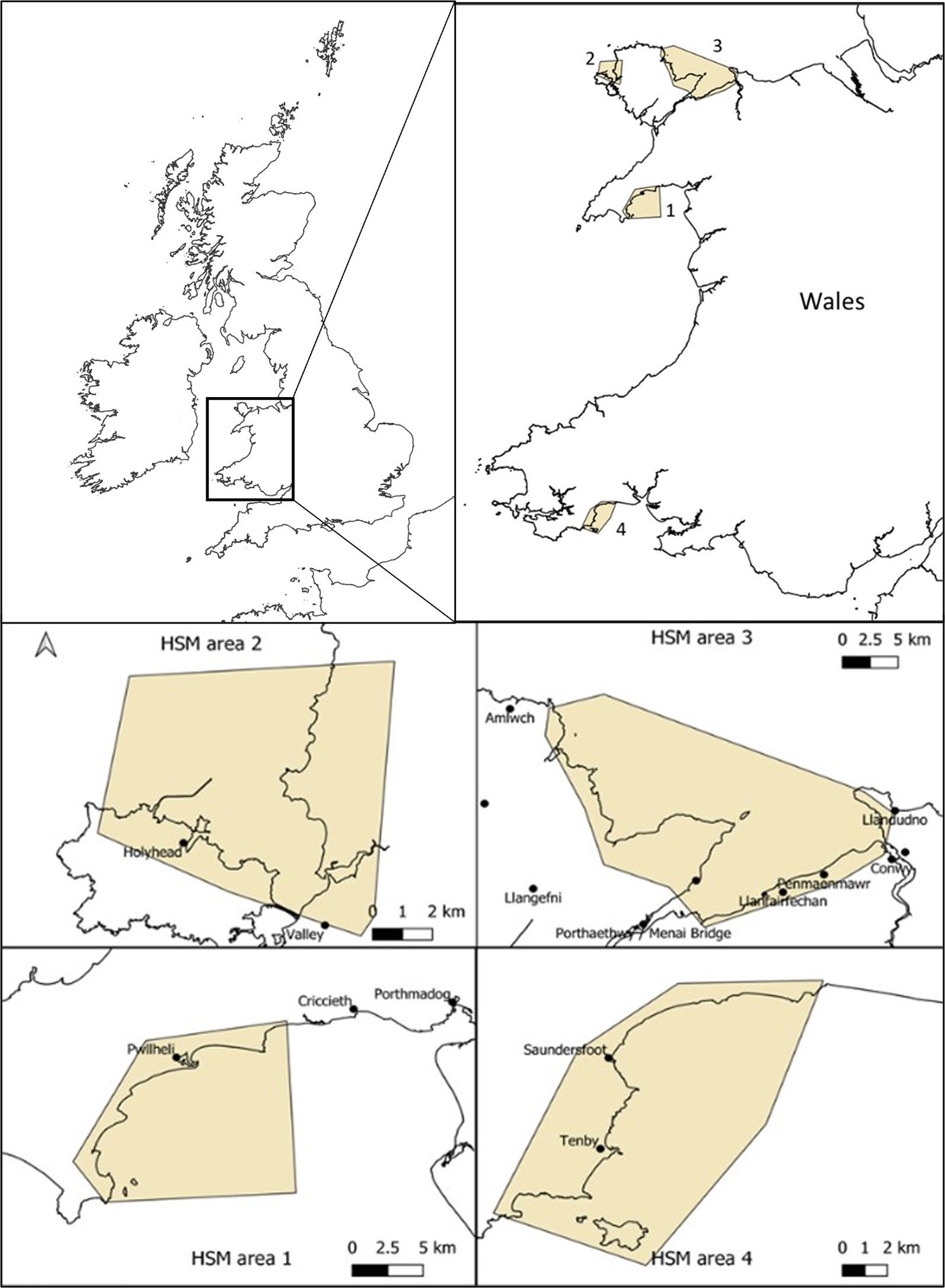
Figure 1 Sites for potential Zostera marina restoration around Wales (UK) used for high resolution habitat suitability modelling using high resolution wave model data. Areas start at Llyn Peninsula, north Wales (area 1), followed by west Anglesey coast (area 2), east Anglesey (area 3) and finally south Wales, Pembrokeshire (area 4).
Our study also sought to improve upon the freely available hydrodynamic data by using wave models to create high resolution wave information over the areas of interest and to compare differences in outputs. Finally, our study used these data sources to produce decision tools for informing seagrass restoration sites from model outputs.
2.2. Zostera marina presence data
To fulfil the aims of this study we sought to obtain presence data for Z. marina around the UK and Ireland from all available sources. This involved checking and refining data points to remove outliers and duplicates. Z. marina presence data were obtained from sources in Table S1, uploaded into QGIS (QGIS Development Team, 2019) and georeferenced. This allows visualisation of data layers and identification of erroneous points such as coordinates that placed records on land or in deep (>20-30m) offshore waters where occurrence of Z. marina is highly unlikely. These points were removed along with duplicate records from the final dataset. Once data were refined, over 2500 presence points remained around the UK, Ireland and the Channel Islands. These point data (Figure 2) were used for testing suitable HSM methods at a broad scale which would then be refined at a smaller spatial scale for potential restoration sites. Polygon data can also be used, but this would limit the number of data sources and require further analysis to get point coordinates needed for the ‘sdm’ package and analysis method used for this study.
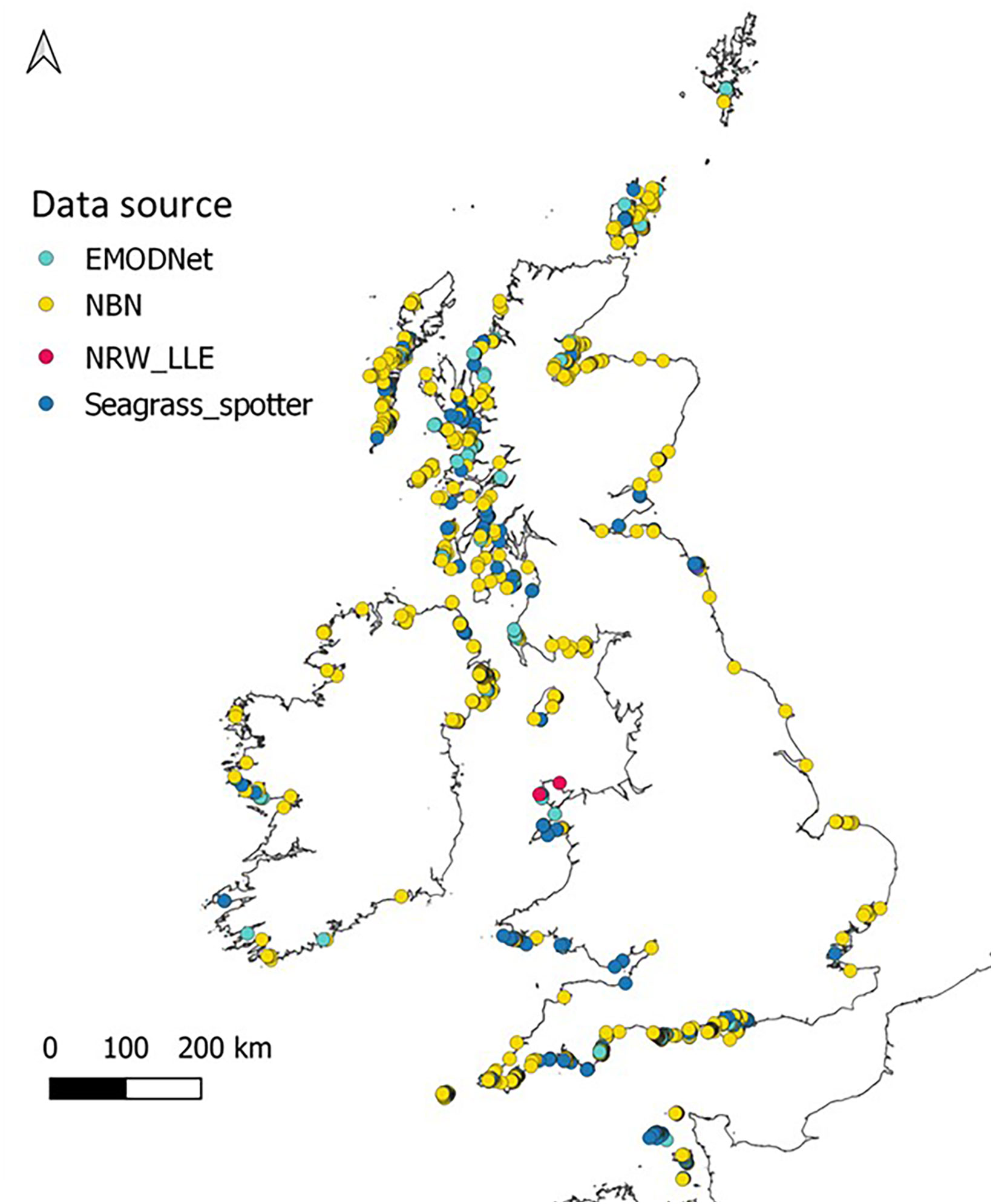
Figure 2 Zostera marina presence around the UK, Ireland and the Channel Islands taken from sources listed in Supplementary Data (Table S1) after outliers were removed.
2.3. Environmental predictor variables for Zostera marina
We obtained the highest resolution freely available environmental data of importance to Z. marina presence for the purpose of refining restoration site choice at a local scale. A review conducted by the authors (Bertelli et al., 2022) identified the most commonly used environmental variables used for predicting seagrass presence using habitat suitability or species distribution modelling. Highest resolution, freely available sources of environmental data were identified. All data were downloaded between September 2020 and February 2021 and covered temporal ranges from 2001 to the time of download (Table S2) and uploaded into QGIS for visualisation.
Environmental data are available in a range of different resolutions, formats and is created using a variety of methods. Photosynthetically available radiation (PAR) at the seabed (From European Marine Observation and Data Network, EMODNet via EUSeaMap) is determined from field and satellite data for light in the water column and then by calculating light attenuation from depth and proximity to coast (EUSeaMap, 2012) at a resolution of ~0.3 km. Wave energy (kinetic energy) at the seabed and kinetic energy from currents at the seabed from EMODNet is based upon modelled outputs from the National Oceanographic Centre (NOC) wave and current models (see EUSeaMap, 2012) to a resolution of ~0.3 km. Data from the Copernicus Marine Environment Monitoring Service (CMEMS, https://www.copernicus.eu/en/services/marine) was used as a source of salinity and temperature as daily averages which are calculated from forecast data which can therefore provide temporal ranges at a resolution of ~1.7 km. Bathymetry was available from EMODNet down to ~70 x 116 m resolution for small high-res downloads, or alternatively from British Oceanographic Data Centre BODC (2020) GEBCO (General Bathymetric Chart of the Oceans) at ~0.2 km. All environmental data layers found to be suitable for habitat suitability modelling are compiled in Supplementary Data (Table S2).
2.4. Data modelling
2.4.1. Broad-scale habitat suitability models
Initial habitat suitability models were developed using openly available environmental data layers and Z. marina presence data for the whole of the British Isles and Ireland. This was to test the effectiveness of model methods using the available environmental data. Environmental data layers were uploaded into R version 4.0.2 (R Core Team, 2020) as raster files along with Z. marina presence point coordinate data as spatial data frames. Five openly available variable datasets were chosen based on suggested predictor variables for seagrass presence identified in Bertelli et al. (2022) - light availability (PAR at seabed), bathymetry, temperature, salinity, wave energy at the seabed and energy from currents at the seabed.
Marine environmental datasets often lack coverage in shallow coastline and pixels covering both land and sea are often excluded (Yesson et al., 2015). To overcome this, a buffering tool was used in QGIS (raster ‘fill nodata’ tool) to interpolate data from neighbouring pixels to cover coastal areas to a distance of 3 pixels. All environmental data layers were resampled using the ‘resample’ function and the nearest neighbour method (‘ngb’) in the ‘raster’ package in R, so they were all the same resolution as the bathymetry layer (15 arc, sec, ~ 0.4 km), extent and format. All the environmental predictor layers were tested for colinearity and colinear variables below a threshold of 0.9 were removed using VIF (Variance Inflation Factor) tests (vifstep and vifcor) in R, recommended for variable selection (Naimi et al., 2014; Guisan et al., 2017). Remaining predictor variables were plotted using pairwise correlation plots to visualise and check no collinearity issues remained.
A suite of methods was used for habitat suitability modelling using the ‘sdm’ package (Naimi and Araújo, 2016) in R. This package allows the use of a wide range of the most common modelling algorithms covering parametric, non-parametric, regression and machine-learning methods to be used all at once. A range of algorithms were chosen to cover the different types of modelling approaches. These included Generalised Linear Models (GLM), Generalised Additive Models (GAM), Multivariate Adaptive Regression Splines (MARS), Random Forest (RF), Boosted Regression Trees (BRT) and Maximum Entropy (MaxEnt), to include some of the most popular methods in other HSM studies (Valle et al., 2013; Guisan et al., 2017; Bertelli et al., 2022). The models follow a formula of seagrass presence as a function of the predictor variables (a stack of the environmental variable layers) using the different approaches. Working only with presence data, the ‘sdm’ software takes a range of randomly sampled ‘background’ points from the study area which are treated as pseudoabsences (Naimi and Araújo, 2016). For the UK and Ireland area, 1050 seagrass presence points were collated with an equal number of pseudoabsences for the HSM. A sample of the presence point data is used to test the model using the bootstrapping method (Naimi and Araújo, 2016). Performance of the models was assessed using area under curve (AUC) of the receiver operating characteristic (ROC) which is produced for each model run (Beca-Carretero et al., 2020). The model-independent variable importance values were also calculated, which are a sensitivity analysis of a model to different predictors (Harisena et al., 2021). This is accomplished by using measures of variable importance that compute a ranking of all the possible species–environment relationships which is one of the most popular measures used (Harisena et al., 2021). Predictions of the probability of presence were then created for each modelling approach. Finally, an ensemble of all the methods (using weighted averages of AUC scores) was used to create prediction outputs in the form of a raster layer indicating probability of suitability for seagrass presence from 0-1 (Naimi and Araujo, 2021).
2.4.2. High resolution wave modelling
To obtain high resolution wave data at each of the four restoration study sites, the openly available computational coastal modelling suite Delft3D was used (Lesser et al., 2004). The Delft3D-WAVE module utilises the third generation spectral SWAN wave model (Booij et al., 1999) to simulate waves in time and space. A Delft3D computational model domain encompassing the Irish Sea with a rectangular 1160 m x 1850 m grid was created to transform offshore waves to the nearshore. High resolution near-shore domains with 50 m x 50 m grid resolution were created for each of the four sites, and nested to the Irish Sea model (Figure 3) to obtain high-resolution wave data required for HSM. Bathymetry for each of the high-resolution domains was created using EMODnet data at 71 m x 116 m resolution. The General Bathymetric Chart of the Oceans (GEBCO) (https://www.gebco.net/data_and_products/gridded_bathymetry_data/) 570 m x 925 m resolution dataset was used to provide additional bathymetry alongside the EMODnet data for the Irish Sea domain. The Irish Sea model was forced by time (hourly) and space-varying (5°) European Centre for Medium-Range Weather Forecasts (ECMWF) ERA5 offshore waves (Hersbach et al., 2018) provided at its offshore boundary. Hourly, 0.5° resolution ERA5 wind data was implemented across the entire model domain to provide atmospheric forcing to the model. Before simulating wave conditions needed for HSM, the Deft3D wave model was validated through a comparison of simulated waves with wave buoy observations at three locations within the larger domain.
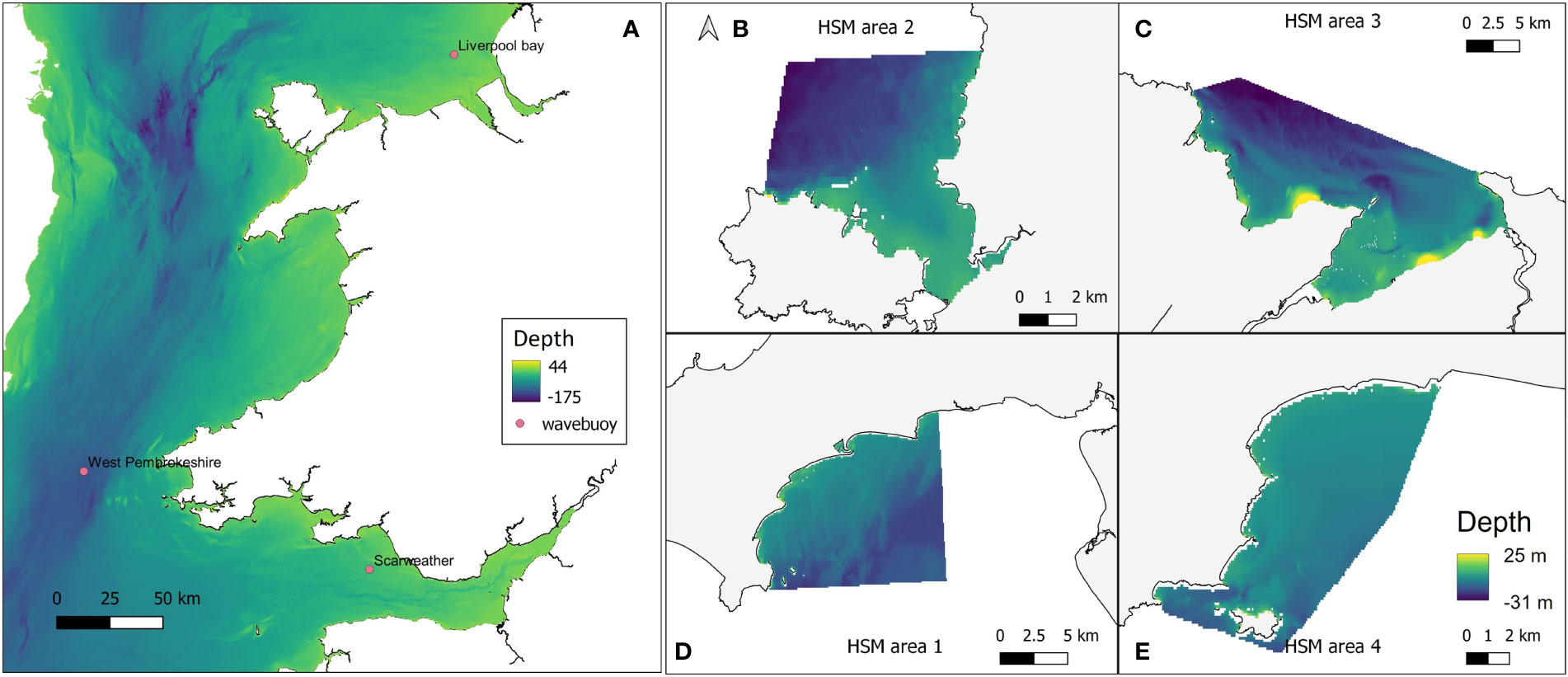
Figure 3 (A) Delft3D Large computational domain and bathymetry, encompassing the Irish Sea and extending towards the Atlantic Ocean. Pink markers indicate the positions of the Scarweather, West Pembrokeshire, and Liverpool Bay wave buoys. Grid cells are 1160 m x1850 m resolution. Nested model domains at (B) West Anglesey (area 2); (C) East Anglesey (area 3); (D) Llyn Peninsula (area 1); and (E) Pembrokeshire (area 4). Bathymetry data were taken from GEBCO and EMODnet datasets. Some topographical areas were also covered in this data layer which explains the high positive values in depth range, but would not have affected outputs as these areas would not be covered by water so were avoided in modelling.
A series of wave simulations were carried out using the validated wave model to provide high resolution data at the four sites. The months January, March, August, and October were run for the years 2015 to 2019 providing a total of 20 model runs. Model outputs including significant wave height, mean and peak wave period, and wave direction are provided at one-hour intervals. The time mean significant wave height was calculated for each simulation period, which will be used in HSM. Figure 4 shows an example of this for January.
2.4.3. Fine-scale habitat suitability models
Wave height data from the near-shore wave models, including mean significant wave height, provided higher resolution data for use in the fine-scale HSM. However, the open-source wave energy (EMODNet) data were also clipped to the restoration areas (Figure 1) so that it could also be used within the final models for comparison between the two. As the high-resolution wave data are calculated based on temporal data, four months were chosen based upon seasons that are significant for the life cycle of Z. marina. These months were: January as a potential for highest impacts due to wave action and wind speeds, March when seed germination and seedling emergence takes place, August for peak biomass and seed production, and October for seed establishment and as such the suitable planting season for restoration work (Sand-Jensen, 1975; Orth and Moore, 1986; Blok et al., 2018). Salinity and temperature data from Copernicus were obtained for each of these months as an average of the daily means. Other data were not temporally resolved so remained as a single data layer (bathymetry, PAR, slope and currents). All environmental data layers were clipped to the areas of interest (HSM areas 1-4, Figure 2) and resampled to the same resolution as the wave height and bathymetry data using the ‘resample’ function and the nearest neighbour method (‘ngb’) in the ‘raster’ package in R. Seagrass presence records were clipped from the original UK dataset for the areas of interest, which resulted in 32 presence points and a higher number of background ‘pseudo-absence’ points (n=90) to improve model performance.
Using VIF (Variance Inflation Factor), all the environmental predictor layers were tested for multicolinearity and variables above a standard threshold of 0.9 were removed, used in many studies (Naimi et al., 2014; Perger et al., 2021; Khan et al., 2022). Remaining predictor variables were also plotted using pairwise correlation plots to screen for collinearity (Supplementary Figure S1).
The nine remaining variable data layers (wave height January, mean temp. March, mean temp. August, mean temp. October, mean salinity August, PAR at seabed, bathymetry, currents and slope) were stacked and used as predictor variables for the HSM. The GAM was found to no longer converge, caused by the increase in the number of variables and low number of observations, so another algorithm was used –flexible discriminate analysis (FDA), which is another regression-based model. This process was repeated by replacing the high-resolution wave height data (Delft3D) with the original open source, low-resolution wave energy data (EMODNet) for comparison between models and variable importance.
Areas of suitable habitat were formatted in QGIS to produce a continuous scale of the model output as a ‘heat-map’ showing probability of suitability (0-1). The layer was then clipped and smoothed to show only the areas with a high probability for both the model results using the low-resolution wave energy data and the high-resolution wave height data. The threshold of 0.6 was chosen as a value that was over 0.5 probability of suitability which returned a reasonable and practical area to work with for future applied restoration. A threshold above 0.6 (0.7 or 0.8) left a considerably reduced area, leaving little scope for practical restoration. A key challenge in the application of HSM is turning the continuous output into a binary output for decision making. We chose 0.6 as an example of this process that practitioners could use but another value could be chosen. Areas of suitable habitat over a threshold of 0.6 were calculated in km2 using the vector calculator function in QGIS.
3. Results
3.1. Results of broad-scale habitat suitability models
For the seagrass presence points around the UK, Ireland and Channel Islands, the mean values for the predictor variables were calculated to provide an estimated niche for seagrass existence. The mean depth for seagrass presence, calculated from bathymetry, was 6.7 m (± 5.4 Standard Deviation), with mean PAR 12.1 Mol.phot.m-2.d-1 (± 8.1 S.D.), wave energy 1671 N.m2.s-1 (± 24577.4 S.D.), energy from currents 119.5 N.m2.s-1 (± 218.5 S.D.), a salinity of 33.8 ppt ( ± 1.7 S.D.) and temperature of 8.4°C (± 1.1 S.D.).
The predictor variables used for the broad-scale HSM were not found to have any collinearity issues. Variable importance was calculated within the ‘sdm’ package in R, using methods outlined in Elith et al. (2005) (Naimi and Araújo, 2016). Bathymetry was the most influential variable (63% based on a correlation matrix - COR, and 32.3% based on Area Under Curve - AUC) followed by PAR at the seabed (Table 1). Results from the ensemble models shown in Supplementary Material, Table S4, show that all model algorithms ran successfully with AUC scores ≥ 0.9, Correlation coefficient ≥ 0.76, and True Summary Statistic (TSS) ≥ 0.73.
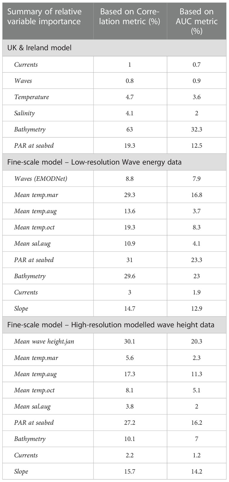
Table 1 Summary of the variable importance based on Correlation metric and AUC for each of the final models, for the broadscale UK and Ireland model, the fine-scale model using lower resolution wave energy data (open source EMODNet) and fine-scale model using high resolution modelled wave height data (Delft3D).
As bathymetry was found to be the variable of highest importance, large regions of shallow seabed around the UK, Ireland and the Channel Islands were predicted as suitable habitat for seagrass (Figure 5). However, this also included areas of coastline exposed to high wave energy (for example, south-west facing coastlines, see Supplementary Material, Figures S3, S4). Wave energy was only found to have 0.8 to 0.9% importance as a predictor variable, which explains why high energy sites were retained as suitable for seagrass growth (Table 1). This highlights the need for better resolution predictor variables, particularly where wave energy or exposure which is known to have a direct effect on seagrass presence.
3.2. Results of high-resolution wave data
Liverpool Bay, West Pembrokeshire, and Scarweather Centre for Environment, Fisheries and Aquaculture Science (CEFAS) wave buoys provided hourly observations around the Welsh coast. The observations during the period 1st March – 31st March 2016 were utilised for model validation, due to the availability of consistent observations at each of the three buoys. Time series of simulated significant wave heights during this period were directly compared with that of the observed wave heights. The comparisons yielded R2 values of 0.87 for the West Pembrokeshire and Scarweather buoys, and 0.93 for the Liverpool Bay buoy, indicating that the computational model is able to accurately simulate waves in the Irish Sea.
In Figure 4, the mean January wave height from across the five January model runs (2015-2019) at each of the four study sites is shown, providing insight into the wave characteristics at each location. At all four sites wave heights were greatest offshore, with the greatest for the more exposed Pembrokeshire site (2-2.5 m), and least for the more sheltered East Anglesey site (1.25-1.35 m). The waves quickly reduce in magnitude as the water depth reduces (Figure 3), and where headlands provide natural shelter from the predominant wave approach. This provides large areas nearshore at each site with mean wave heights between 0.5-1 m depending on the site.
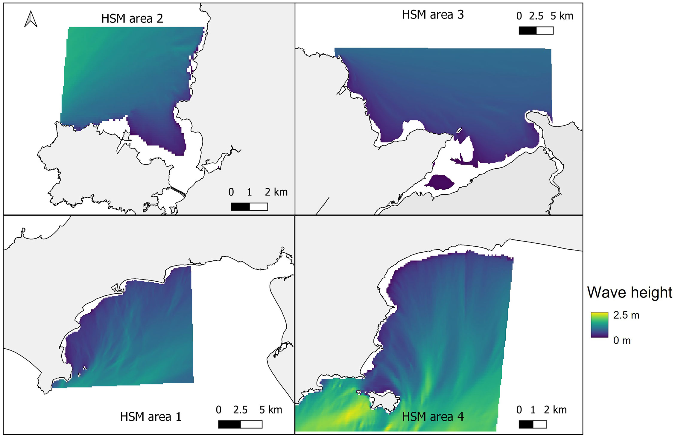
Figure 4 Mean significant wave height from across the five January model runs (2015-2019) at the four selected sites. Top left – West Anglesey (area 2), top right – East Anglesey (area 3), bottom left – Llyn Peninsula (area 1), bottom right – Pembrokeshire (area 4).
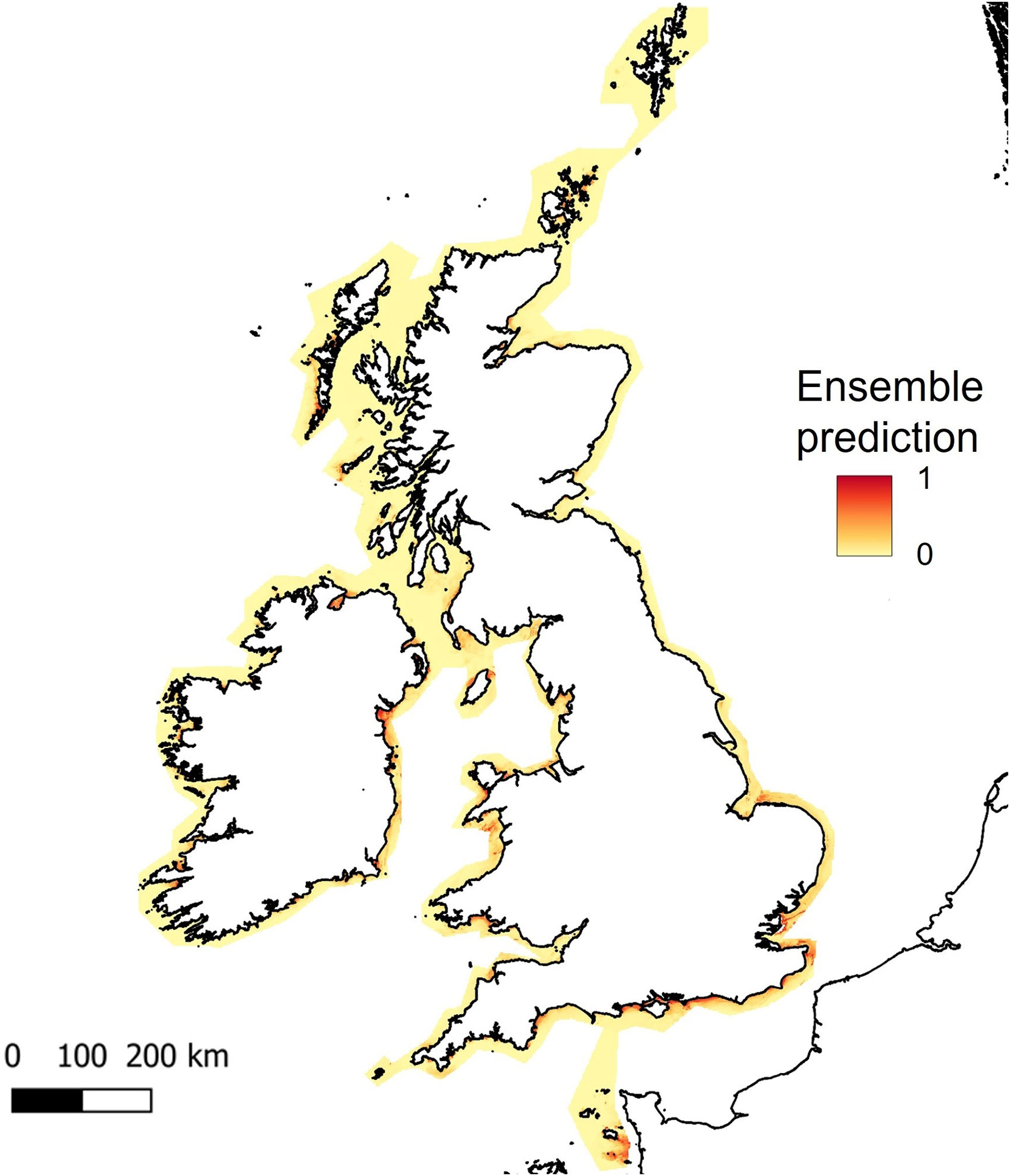
Figure 5 Predicted habitat suitability for Zostera marina, based on ensemble model results for UK, Ireland and Channel Isles. The legend shows colour scale for the probability of habitat suitability from yellow (low) to red (high).
3.3. Results of fine-scale habitat suitability models
Many of the mean values for the predictor variables restricted to the seagrass presence in the local restoration areas varied substantially from the broad-scale data. The mean depth for seagrass presence was considerably lower at 0.4 m (± 3.5 S.D), wave energy at 160 N.m2.s-1 (± 403.3 S.D.) and energy from currents 51.2 N.m2.s-1 (± 68.8 S.D). Optimal PAR was only slightly higher at 14.1 Mol.phot.m-2.d-1 (± 7.3 S.D.) than for the broad-scale seagrass presence. Salinity, temperature, and modelled wave height varied depending on monthly average (see Supplementary Data, Table S3). Mean temperature ranged from 7.7°C in January to 18.7°C in August. Salinity ranged from 30.4 ppt in January to 31.7 ppt in March. Average slope that was calculated from the higher resolution bathymetry data was found to be 89.9°.
Removal of colinear variables left mean wave height for January; mean temperature for March; mean temperature for August; mean temperature for October; mean salinity for August; PAR at seabed; Bathymetry; Energy at seabed due to currents and Slope of seabed. All remaining predictor variables showed a pairwise correlation below 0.7 (Supplementary Material, Figure S1). Variable importance changed significantly in the fine-scale models in comparison to the broadscale models, with wave height becoming much more influential in predicting seagrass presence (Table 1, Supplementary Material, Figure S2). The resulting predictions for suitable habitat for Z. marina are shown in Figure 6 for each of the restoration site areas around Wales, with model results shown Supplementary Material, Table S4. All model algorithms resulted in AUC scores of equal to or greater than 0.9 which can be interpreted as good or even excellent predictions based on scales defined in other studies (Araujo et al., 2005). The TSS (True Summary Statistic) is also a useful model validation measure which is independent of prevalence or size of dataset, a limitation for the smaller restoration areas where presence data is low (Allouche et al., 2006). TSS values closer to 1 show higher prediction accuracy, and all models scored above 0.8. Random forest (RF) was found to perform the best (AUC 0.98 ± 0.03 S.D., COR 0.83 ± 0.06 S.D. and TSS 0.95 ± 0.09 S.D.) and flexible discriminate analysis (FDA) the lowest scoring (AUC 0.9 ± 0.03 S.D., COR 0.54 ± 0.17 SD and TSS 0.82 ± 0.1 S.D.). Mean wave height (January) was the most important variable based on the average correlation metric (30.1% ± 24.9 S.D.) and the AUC metric (20.3% ± 20.8 S.D.) for all model runs, followed by PAR at seabed (COR 27.2%, AUC 16.2%, see Table 1).
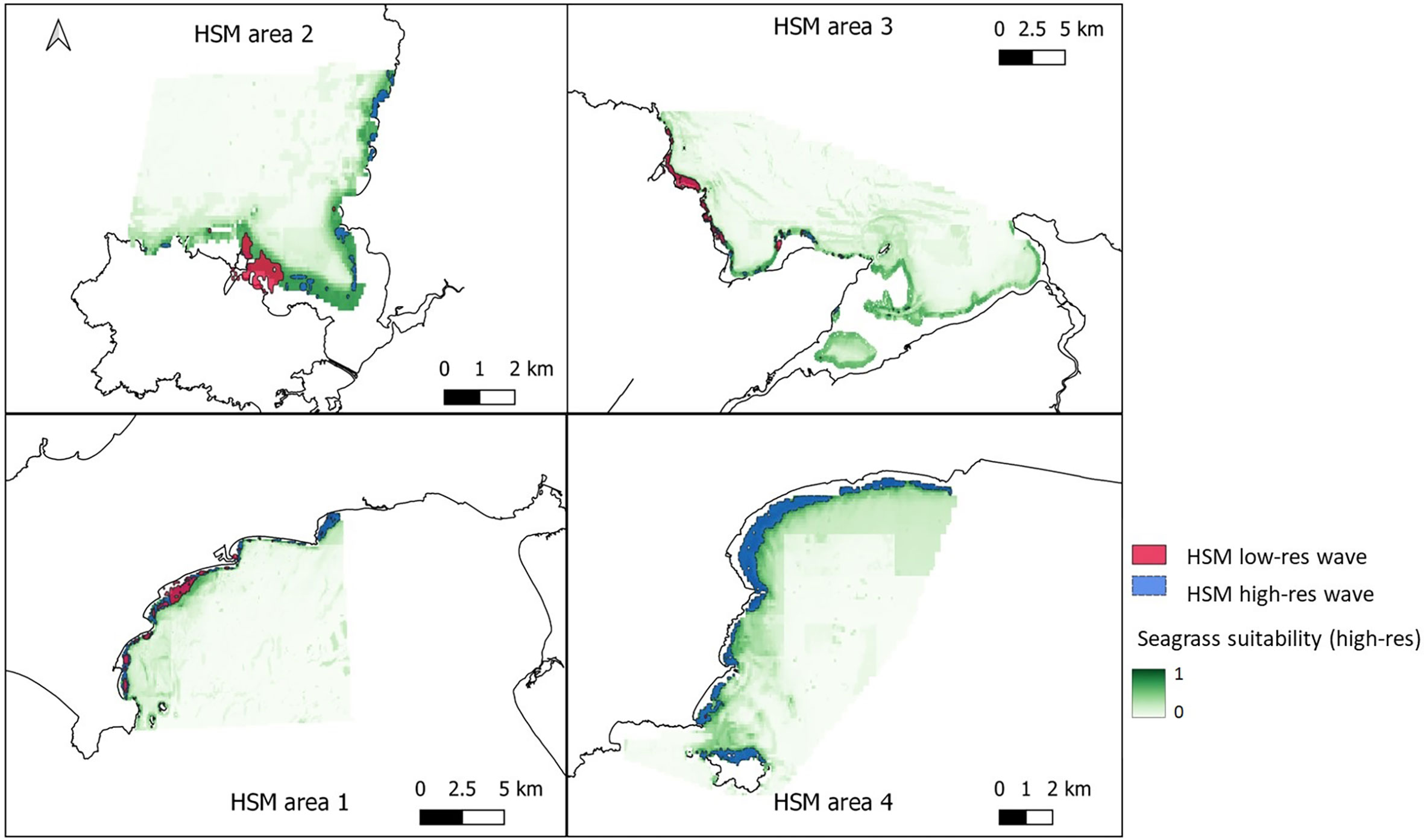
Figure 6 Areas of suitable seagrass habitat in green for the four chosen areas around Wales. Top left – West Anglesey (area 2), top right – East Anglesey (area 3), bottom left – Llyn Peninsula (area 1), bottom right – Pembrokeshire (area 4). Maps shows results from ensemble model of 6 methods, using presence only data and all the non-colinear variables including high-resolution wave height data. Overlayed is the vector layer outputs when a threshold of >0.6 probability was applied to the model with low resolution wave data model (pink) and high-resolution wave data model (blue) for comparison.
When the model was repeated with the low-resolution wave energy data in place of the high-resolution wave height data, PAR at the seabed (COR 31% ± 0.3 S.D., AUC 23% ± 0.2 SD), bathymetry (COR 29.6% ± 0.2 SD, AUC 23% ± 0.2 S.D.) and mean temperature in March (COR 29.3% ± 0.3 SD, AUC 16.8% ± 0.3 S.D.) were the most important variables influencing habitat suitability (Table 1). AUC, COR and TSS scores were lower in the model runs when the lower resolution wave energy data was substituted suggesting the model fits were not as successful as when high resolution wave height data was included. Only two methods had an AUC mean score over 0.9 (FDA 0.96 ± 0.05 S.D. and MaxENT 0.92 ± 0.06 S.D.) and none scored a TSS value ≥ 0.8 (Supplementary Material, Table S4).
Figures 6, 7 shows areas with probability ≥ 0.6 of being suitable for Z. marina presence for the ensemble model using low-resolution wave energy data and the high-resolution wave height data for the different areas. The total suitable area ≥ 0.6 predicted from the HSM using the high-resolution wave data was more than twice (13.69 km2) the predicted area from the HSM using the low-resolution wave energy data (6.17C, Figures 6, 7). Within the same areas, the area predicted to be ≥ 0.6 suitable for seagrass from the broad-scale model was 92.3 km2.
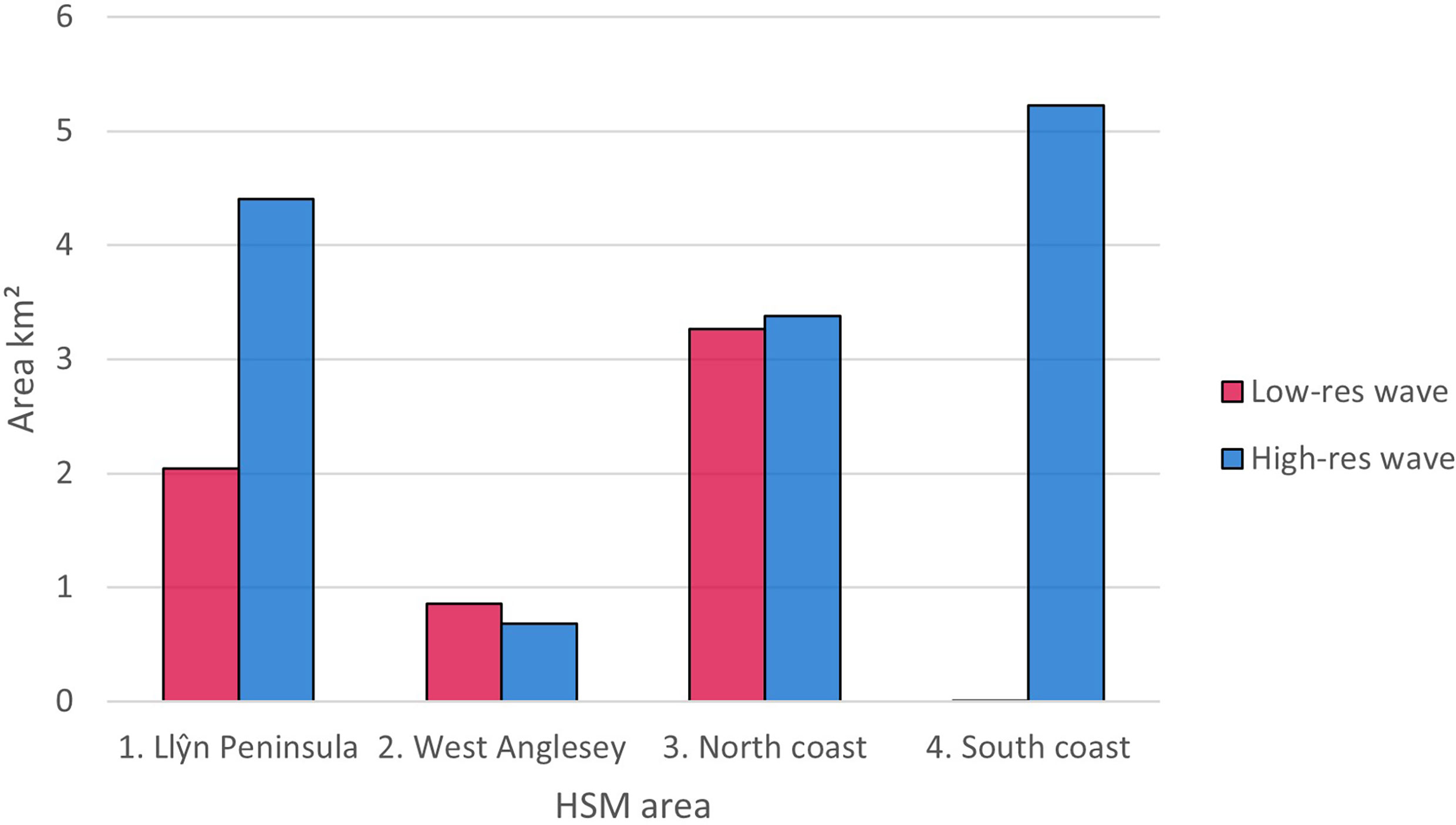
Figure 7 Difference in area (km2) predicted as suitable using ≥0.6 probability threshold for ensemble models using lower resolution wave energy data and high-resolution wave height data.
4. Discussion
Determining where to invest limited financial resources for restoration or environmental enhancement of species or habitats requires appropriate decision support tools. Habitat suitability models are a useful tool for assisting with this process by identifying areas where species and habitats should be able to exist based upon the environmental data that are available. Here we provide a novel case study that illustrates how the creation of high-resolution environmental datasets, and the use of ensemble modelling techniques can lead to more refined HSMs that better predict these windows of opportunity for restoration, ultimately leading to a reduction in environmental and financial risk attached to major ecological improvement projects.
Our study finds that potential seagrass restoration areas can be defined to a much finer scale and more ecologically representative level by incorporating targeted fine resolution Delft3D wave data in marine habitat suitability models. Model validation results were good for the initial broad-scale models using open access environmental datasets, however the map outputs overpredicted suitability in areas that would not be appropriate for seagrass growth, such as very large swathes of exposed coastlines around Anglesey Island (Natural Resources Wales, 2009) and deep (>15 m) regions such as offshore from the mid Wales coast with wave energy the second to least important variable. The lower resolution of the environmental data available at a broader scale will still identify suitable regions for seagrass growth but the spatial overlap at this scale makes it more difficult for differentiating where conditions are most suitable within smaller areas.
The results of the ensemble model using Delft3D wave data appear to show appropriate predictions for seagrass growth at a fine scale due to the higher resolution environmental predictors of wave height and bathymetry. Mean wave height for January obtained from the wave model was found to be the most important variable for predicting seagrass suitability which is the month predicted to have the highest wave heights and with suitability increasing as wave height decreases. PAR at the seabed was the second most important variable for predicting seagrass presence in the four areas around Wales.
The open-source wave energy data used in the same ensemble model was less important as a predictor variable, with slope and bathymetry the most important factors. The resulting areas predicted to be highly suitable for seagrass growth was found to be more than 50% lower when using the low-resolution wave data.
The use of ensemble modelling allowed a combination of several model methods to provide predictions which will be more robust to uncertainties that may arise from using a single method (Araújo and New, 2007; Latif et al., 2013). This removes the need for selecting a single ‘best’ model which limits model selection bias and reduces the need for removing predictor variables which is often the case for step-wise model selection. This method is useful for predictions in new areas where conditions may be different or where data are lacking (Guisan et al., 2017).
The interpretation of HSM outputs can be relatively subjective based upon prior knowledge of sites and the species in question. The AUC, COR and TSS scores allow model comparisons and will indicate those which best fit, however when the outputs are very similar, visual interpretation is needed to assess if the results are realistic. The model results show higher AUC, COR and TSS scores when the high-resolution wave height data were included for the smaller potential restoration areas. More areas were suitable in areas 1 and 4, on the Llyn Peninsula and southwest Wales coast, than the Anglesey and north coast areas (2 and 3). This could be due to areas 2 and 3 having higher areas of intertidal shoreline. Due to large resource requirements, the wave model within Delft3D was not coupled to the tidal processes, and as such wave modelling was carried out for the mean water level. The wave modelling therefore does not provide data in the upper intertidal, limiting prediction of wave heights in shallow extents, especially where land is also obstructing potential wave energy, and therefore this restricts the model areas to subtidal zones. However, this issue was consistent with other open-source environmental data such as PAR at the seabed, which highlights the difficulties in extending marine HSMs into intertidal areas. The wave height data were extrapolated to provide overlap in the shallows, but only by 3 pixels to maintain data integrity as was carried out for other environmental data layers. It can also be argued that the use of high-resolution wave data is only really of use in areas that are more affected by wave action, such as an open bay where there is some gradient of wave exposure such as areas 1 and 4. It is possibly not so effective in areas that are heavily sheltered from prevailing waves e.g. within an archipelago, or in a north-east facing enclosed bay where other hydrodynamics may be having more impact (e.g. tides and currents), which could be the case for the shallow areas around Anglesey - areas 2 and 3. The best way of testing this is to trial restoration in the sites and compare results from the different outputs such as outlined by Thom et al. (2018) which is the next step. Nonetheless, the results do show where restoration should be more successful due to the environmental conditions in all the areas and will provide a good baseline for selecting sites for restoration in the future. This study method provides evidence that the use of high-resolution wave data such as the Delft3D used in this study, can improve model outputs and highlights the importance of wave exposure as a factor in determining seagrass presence.
5. Conclusions
Habitat suitability modelling is a valuable tool for the purposes of conservation management and realising the risks of climate change on key species but also for aiding in decision making for the restoration of our marine systems. This study shows the benefits to obtaining high resolution predictor variable data for HSM at small regional scales. For predicting suitable conditions for seagrass, wave height data at a higher resolution was found to be the most important variable and model outputs were improved and differed considerably in comparison to the use of low-resolution wave energy data in its place. However, it should also be recognised that there is a lack of availability of many environmental variable data for the shallow coastal, including intertidal, areas. This has implications for improving HSM for restoration enabling efforts to be focused on areas where the chance of success will be highest.
Data availability statement
The original contributions presented in the study are included in the article/Supplementary Material. Further inquiries can be directed to the corresponding author.
Author contributions
CB: writing – original draft, methodology, investigation, data curation, formal analysis and validation. WB: writing - methodology, data curation, formal analysis and validation. DR, HK, JB, and RU: conceptualization, investigation – review and editing. RU, JB, HK, and DR: funding acquisition, supervision, methodology. All authors contributed to the article and approved the submitted version.
Funding
Initial study was funded by WWF and Sky Seagrass Ocean Rescue project with follow up funding from ReSOW NERC funding NE/V01711X/1 to continue and complete the investigation.
Acknowledgments
This study has been conducted using E.U. Copernicus Marine Service Information; https://doi.org/10.48670/moi-00054 and from EMODNet - Licensed under CC-BY 4.0 from the European Marine Observation and Data Network (EMODnet) Seabed Habitats initiative (www.emodnet-seabedhabitats.eu), funded by the European Commission.
Conflict of interest
The authors declare that the research was conducted in the absence of any commercial or financial relationships that could be construed as a potential conflict of interest.
Publisher’s note
All claims expressed in this article are solely those of the authors and do not necessarily represent those of their affiliated organizations, or those of the publisher, the editors and the reviewers. Any product that may be evaluated in this article, or claim that may be made by its manufacturer, is not guaranteed or endorsed by the publisher.
Supplementary material
The Supplementary Material for this article can be found online at: https://www.frontiersin.org/articles/10.3389/fmars.2022.1004829/full#supplementary-material
References
Adams M. P., Saunders M. I., Maxwell P. S., Tuazon D., Roelfsema C. M., Callaghan D. P., et al. (2016). Prioritizing localized management actions for seagrass conservation and restoration using a species distribution model. Aquat. Conserv. Mar. Freshw. Ecosyst. 26, 639–659. doi: 10.1002/aqc.2573
Allouche O., Tsoar A., Kadmon R. (2006). Assessing the accuracy of species distribution models: Prevalence, kappa and the true skill statistic (TSS). J. Appl. Ecol. 43, 1223–1232. doi: 10.1111/j.1365-2664.2006.01214.x
Araújo M. B., Anderson R. P., Barbosa A. M., Beale C. M., Dormann C. F., Early R., et al. (2019). Standards for distribution models in biodiversity assessments. Sci. Adv. 5, 1–12. doi: 10.1126/sciadv.aat4858
Araújo M. B., New M. (2007). Ensemble forecasting of species distributions. Trends Ecol. Evol. 22, 42–47. doi: 10.1016/j.tree.2006.09.010
Araujo M., Pearson R., Thuiller W., Erhard M. (2005). Validation of species-climate impact models under climate change. Glob. Change Biol. 11, 1504–1513. doi: 10.1111/j.1365-2486.2005.001000.x
Beca-Carretero P., Varela S., Stengel D. B. (2020). A novel method combining species distribution models, remote sensing, and field surveys for detecting and mapping subtidal seagrass meadows. Aquat. Conserv. Mar. Freshw. Ecosyst. 30, 1098–1110. doi: 10.1002/aqc.3312
Bertelli C. M., Stokes H. J., Bull J. C., Unsworth R. K. F. (2022). The use of habitat suitability modelling for seagrass: A review. Front. Mar. Sci. doi: 10.3389/fmars.2022.997831
Bertelli C. M., Unsworth R. K. F. (2018). Light stress responses by the eelgrass, zostera marina (L). Front. Environ. Sci. 6. doi: 10.3389/fenvs.2018.00039
Blok S. E., Olesen B., Krause-Jensen D. (2018). Life history events of eelgrass zostera marina l. populations across gradients of latitude and temperature. Mar. Ecol. Prog. Ser. 590, 79–93. doi: 10.3354/meps12479
Booij N., Ris R. C., Holthuijsen L. H. (1999). A third-generation wave model for coastal regions 1. model description and validation. J. Geophys. Res. Ocean. 104, 7649–7666. doi: 10.1029/98JC02622
Danovaro R., Aronson J., Cimino R., Gambi C., Snelgrove P. V. R., Van Dover C. (2021). Marine ecosystem restoration in a changing ocean. Restor. Ecol. 29, 1–8. doi: 10.1111/rec.13432
D’Avack E. A. S., Tyler-Walters H., Wilding C., Garrard S. M. (2019). “Zostera (Zostera) marina beds on lower shore or infralittoral clean or muddy sand,” in Marine life information network: Biology and sensitivity key information reviews. Eds. Tyler-Walters H., Hiscock K. Available at: https://www.marlin.ac.uk/habitats/detail/257.
Davison D. M., Hughes D. J. (1998). Zostera biotopes 1. an overview of dynamic and sensitivity characteristics for conservation management of marine SACs.
Dennison W. C., Alberte R. S. (1985). Role of daily light period in the depth distribution of zostera marina (eelgrass). Mar. Ecol. Prog. Ser. 25, 51–61. doi: 10.3354/meps025051
Duarte C. M. (1991). Seagrass depth limits. Aquat. Bot. 40, 363–377. doi: 10.1016/0304-3770(91)90081-F
Elith J., Ferrier S., Huettmann F., Leathwick J. (2005). The evaluation strip: A new and robust method for plotting predicted responses from species distribution models. Ecol. Model. 186 (3), 280–289.
Fonseca M. S., Bell S. S. (1998). Influence of physical setting on seagrass landscapes. Mar. Ecol. Prog. Ser. 171, 109–121. doi: 10.3354/meps171109
Furman B. T., Peterson B. J. (2015). Sexual recruitment in zostera marina: Progress toward a predictive model. PloS One 10, 1–20. doi: 10.1371/journal.pone.0138206
Gamble C., Debney A., Glover A., Bertelli C., Green B., Hendy I., et al. (2021). Seagrass restoration handbook UK & Ireland.
GEBCO Bathymetric Compilation Group 2020 (2020). “The GEBCO_2020 grid - a continuous terrain model of the global oceans and land,” (NERC, UK: British Oceanographic Data Centre, National Oceanography Centre). doi: 10.5285/a29c5465-b138-234d-e053-6c86abc040b9
Green A. E., Unsworth R. K. F., Chadwick M. A., Jones P. J. S. (2021). Historical analysis exposes catastrophic seagrass loss for the united kingdom. Front. Plant Sci. 12. doi: 10.3389/fpls.2021.629962
Guisan A., Thuiller W., Zimmermann N. E. (2017). Habitat suitability and distribution models: With applications in R (ecology, biodiversity and conservation) (Cambridge: Cambridge University Press). doi: 10.1017/9781139028271
Harisena N. V., Groen T. A., Toxopeus A. G., Naimi B. (2021). When is variable importance estimation in species distribution modelling affected by spatial correlation? Ecography (Cop.). 44, 778–788. doi: 10.1111/ecog.05534
Hersbach H., Bell B., Berrisford P., Biavati G., Horányi A., Muñoz Sabater J., et al. (2018). ERA5 hourly data on single levels from 1979 to present (Copernicus Climate Change Service (C3S) Climate Data Store (CDS). doi: 10.24381/cds.adbb2d47
Hu W., Zhang D., Chen B., Liu X., Ye X., Jiang Q., et al. (2021). Mapping the seagrass conservation and restoration priorities: Coupling habitat suitability and anthropogenic pressures. Ecol. Indic. 129, 107960. doi: 10.1016/j.ecolind.2021.107960
Infantes E., Eriander L., Moksnes P. (2016). Eelgrass (Zostera marina) restoration on the west coast of Sweden using seeds. Mar. Ecol. Prog. Ser. 546, 31–45. doi: 10.3354/meps11615
Infantes E., Orfila A., Bouma T. J., Simarro G., Terrados J. (2011). Posidonia oceanica and cymodocea nodosa seedling tolerance to wave exposure. Limnol. Oceanogr. 56, 2223–2232. doi: 10.4319/lo.2011.56.6.2223
Jackson E. L., Griffiths C. A., Durkin O. (2013). A guide to assessing and managing anthropogenic impact on marine angiosperm habitat - part 1: Literature review. Natural Engl. Commissioned Rep.
Khan Z., Ali S. A., Parvin F., Mohsin M., Shamim S. K., Ahmad A. (2022). Predicting the effects of climate change on prospective banj oak (Quercus leucotrichophora) dispersal in kumaun region of uttarakhand using machine learning algorithms. Model. Earth Syst. Environ. doi: 10.1007/s40808-022-01485-5
Koch E. W., Sanford L. P., Chen S.-N., Shafer D. J., Smith J. M. (2006). System-wide water resources research program and submerged aquatic vegetation restoration research program (Waves in seagrass Systems : Review and technical recommendations). Eng. Res. Dev. Cent.
Koch E. W., Verduin J. J., Katwijk V. (2001). Measurements of physical parameters in seagrass habitats. Glob. Seagrass Res. Methods, 325–344. doi: 10.1016/B978-044450891-1/50018-9
Krause-Jensen D., Pedersen M. F., Jensen C. (2003). Regulation of eelgrass (Zostera marina) cover along depth gradients in Danish coastal waters. Estuaries 26, 866–877. doi: 10.1007/BF02803345
Kuusemäe K., Rasmussen E. K., Canal-Vergés P., Flindt M. R. (2016). Modelling stressors on the eelgrass recovery process in two Danish estuaries. Ecol. Modell. 333, 11–42. doi: 10.1016/j.ecolmodel.2016.04.008
Latif Q. S., Saab V. A., Dudley J. G., Hollenbeck J. P. (2013). Ensemble modeling to predict habitat suitability for a large-scale disturbance specialist. Ecol. Evol. 3, 4348–4364. doi: 10.1002/ece3.790
Lee K.-S., Park S. R., Kim Y. K. (2007). Effects of irradiance, temperature, and nutrients on growth dynamics of seagrasses: A review. J. Exp. Mar. Bio. Ecol. 350, 144–175. doi: 10.1016/j.jembe.2007.06.016
Lesser G. R., Roelvink J. A., van Kester J. A. T. M., Stelling G. S. (2004). Development and validation of a three-dimensional morphological model. Coast. Eng. 51, 883–915. doi: 10.1016/j.coastaleng.2004.07.014
Marion S. R., Orth R. J., Fonseca M., Malhotra A. (2021). Seed burial alleviates wave energy constraints on zostera marina (Eelgrass) seedling establishment at restoration-relevant scales. Estuaries Coasts 44 (2), 352–366. doi: 10.1007/s12237-020-00832-y
Marsh J., Dennison W. C., Alberte R. S. (1986). Effects of temperature on photosynthesis and respiration in eelgrass (Zostera marina l.). J. Exp. Mar. Bio. Ecol. 101, 257–267. doi: 10.1016/0022-0981(86)90267-4
McKenzie L. J., Nordlund L. M., Jones B. L., Cullen-Unsworth L. C., Roelfsema C., Unsworth R. K. F. (2020). The global distribution of seagrass meadows. Environ. Res. Lett. 15, 074041. doi: 10.1088/1748-9326/ab7d06
Moore K. A., Jarvis J. C. (2008). Environmental factors affecting recent summertime eelgrass diebacks in the lower Chesapeake bay: implications for long-term persistence. J. Coastal Res. 2008 (10055), 135–147. doi: 10.2112/SI55-014
Naimi B., Araújo M. B. (2016). Sdm: A reproducible and extensible r platform for species distribution modelling. Ecography (Cop.). 39, 368–375. doi: 10.1111/ecog.01881
Naimi B., Hamm N. A. S., Groen T. A., Skidmore A. K., Toxopeus A. G. (2014). Where is positional uncertainty a problem for species distribution modelling? Ecography (Cop.). 37, 191–203. doi: 10.1111/j.1600-0587.2013.00205.x
Nielsen S., Sand-Jensen K., Borum J., Geertz-Hansen O. (2002). Depth colonization of eelgrass (Zostera marina) and macroalgae as determined by water transparency in Danish coastal waters. Estuaries Coasts 25, 1025–1032. doi: 10.1007/bf02691349
Orth R. J., Moore K. A. (1986). Seasonal and year-to-year variations in the growth of zostera marina l. (eelgrass) in the lower Chesapeake bay. Aquat. Bot. 24, 335–341. doi: 10.1017/CBO9781107415324.004
Peralta G., Brun F. G., Pérez-Lloréns J. L., Bouma T. J. (2006). Direct effects of current velocity on the growth, morphometry and architecture of seagrasses: A case study on Zostera noltii. Mar. Ecol. Prog. Ser. 327, 135–142.
Perger R., do Amaral K. B., Bianchi F. M. (2021). Distribution modelling of the rare stink bug ceratozygum horridum (Germar 1839): isolated in small spots across the neotropics or a continuous population? J. Nat. Hist. 55, 649–663. doi: 10.1080/00222933.2021.1919328
QGIS Development Team (2019). “Open source geospatial foundation project,” in QGIS geographic information system. Available at: http://qgis.osgeo.org.
Rowden A. A., Anderson O. F., Georgian S. E., Bowden D. A., Clark M. R., Pallentin A., et al. (2017). High-resolution habitat suitability models for the conservation and management of vulnerable marine ecosystems on the Louisville seamount chain, south pacific ocean. Front. Mar. Sci. 4. doi: 10.3389/fmars.2017.00335
Salo T., Pedersen M. F., Boström C. (2014). Population specific salinity tolerance in eelgrass (Zostera marina). J. Exp. Mar. Bio. Ecol. 461, 425–429. doi: 10.1016/j.jembe.2014.09.010
Sand-Jensen K. (1975). Biomass, net production and growth dynamics in an eelgrass (Zostera marina l.) population in vellerup vig, Denmark. Ophelia 14, 185–201. doi: 10.1080/00785236.1975.10422501
Short F., Carruthers T., Dennison W., Waycott M. (2007). Global seagrass distribution and diversity: A bioregional model. J. Exp. Mar. Bio. Ecol. 350, 3–20. doi: 10.1016/j.jembe.2007.06.012
Stevens A. W., Lacy J. R. (2012). The influence of wave energy and sediment transport on seagrass distribution. Estuar. Coasts 35 (1), 92–108.
Temmink R. J. M., Christianen M. J. A., Fivash G. S., Angelini C., Boström C., Didderen K., et al. (2020). Mimicry of emergent traits amplifies coastal restoration success. Nat. Commun. 11, 1–9. doi: 10.1038/s41467-020-17438-4
Thompson K., Jackson E., Kakkonen J. (2014). Seagrass (Zostera) beds in Orkney. Scottish Nat. Herit. Commun.
Thom R., Gaeckle J., Buenau K., Borde A., Vavrinec J., Aston L., et al. (2018). Eelgrass (Zostera marina l.) restoration in Puget Sound: Development of a site suitability assessment process. Restor. Ecol. 26 (6), 1066–1074.
Valle M., Chust G., del Campo A., Wisz M. S., Olsen S. M., Garmendia J. M., et al. (2014). Projecting future distribution of the seagrass zostera noltii under global warming and sea level rise. Biol. Conserv. 170, 74–85. doi: 10.1016/j.biocon.2013.12.017
Valle M., van Katwijk M. M., de Jong D. J., Bouma T. J., Schipper A. M., Chust G., et al. (2013). Comparing the performance of species distribution models of zostera marina: Implications for conservation. J. Sea Res. 83, 56–64. doi: 10.1016/j.seares.2013.03.002
Van Katwijk M. M. M., Bos A. R. R., de Jonge V. N. N., Hanssen L. S. A. M., Hermus D.C.R.C.R., de Jong D. J. J. (2009). Guidelines for seagrass restoration: Importance of habitat selection and donor population, spreading of risks, and ecosystem engineering effects. Mar. pollut. Bull. 58, 179–188. doi: 10.1016/j.marpolbul.2008.09.028
van Katwijk M. M., Hermus D. C. R. (2000). Effects of water dynamics on zostera marina: Transplantation experiments in the intertidal Dutch wadden Sea. Mar. Ecol. Prog. Ser. 208, 107–118. doi: 10.3354/meps208107
Waltham N. J., Elliott M., Lee S. Y., Lovelock C., Duarte C. M., Buelow C., et al. (2020). UN Decade on ecosystem restoration 2021–2030—What chance for success in restoring coastal ecosystems? Front. Mar. Sci. 7. doi: 10.3389/fmars.2020.00071
Keywords: seagrass, restoration, habitat suitability modelling, Delft-3D wave modelling, Zostera marina
Citation: Bertelli CM, Bennett WG, Karunarathna H, Reeve DE, Unsworth RKF and Bull JC (2023) High-resolution wave data for improving marine habitat suitability models. Front. Mar. Sci. 9:1004829. doi: 10.3389/fmars.2022.1004829
Received: 27 July 2022; Accepted: 13 December 2022;
Published: 06 January 2023.
Edited by:
Junyu He, Zhejiang University, ChinaReviewed by:
Matteo Zucchetta, National Research Council (CNR), ItalyBradley Thomas Furman, Florida Fish and Wildlife Research Institute, United States
Copyright © 2023 Bertelli, Bennett, Karunarathna, Reeve, Unsworth and Bull. This is an open-access article distributed under the terms of the Creative Commons Attribution License (CC BY). The use, distribution or reproduction in other forums is permitted, provided the original author(s) and the copyright owner(s) are credited and that the original publication in this journal is cited, in accordance with accepted academic practice. No use, distribution or reproduction is permitted which does not comply with these terms.
*Correspondence: Chiara M. Bertelli, Yy5tLmJlcnRlbGxpQHN3YW5zZWEuYWMudWs=