ENSO coupling to the equatorial Atlantic: Analysis with an extended improved recharge oscillator model

Introduction: Observational and modeling studies have examined the interactions between El Niño-Southern Oscillation (ENSO) and the equatorial Atlantic variability as incorporated into the classical charge-recharge oscillator model of ENSO. These studies included the role of the Atlantic in the predictability of ENSO but assumed stationarity in the relationships, i.e., that models’ coefficients do not change over time. A recent work by the authors has challenged the stationarity assumption in the ENSO framework but without considering the equatorial Atlantic influence on ENSO.

Methods: The present paper addresses the changing relationship between ENSO and the Atlantic El Niño using an extended version of the recharge oscillator model. The classical two-variable model of ENSO is extended by adding a linear coupling on the SST anomalies in the equatorial Atlantic. The model’s coefficients are computed for different periods. This calculation is done using two methods to fit the model to the data: (1) the traditional method (ReOsc), and (2) a novel method (ReOsc+) based on fitting the Fisher’s Z transform of the auto and cross-correlation functions.

Results: We show that, during the 20th century, the characteristic damping rate of the SST and thermocline depth anomalies in the Pacific have decreased in time by a factor of 2 and 3, respectively. Moreover, the damping time of the ENSO fluctuations has doubled from 10 to 20 months, and the oscillation period of ENSO has decreased from 60-70 months before the 1960s to 50 months afterward. These two changes have contributed to enhancing ENSO amplitude. The results also show that correlations between ENSO and the Atlantic SST strengthened after the 70s and the way in which the impact of the equatorial Atlantic is added to the internal ENSO variability.

Conclusions: The remote effects of the equatorial Atlantic on ENSO must be considered in studies of ENSO dynamics and predictability during specific time-periods. Our results provide further insight into the evolution of the ENSO dynamics and its coupling to the equatorial Atlantic, as well as an improved tool to study the coupling of climatic and ecological variables.

1 Introduction

El Niño and the Southern Oscillation (ENSO) is the most important climate variability mode with worldwide impacts (Philander, 1990; Trenberth, 2002; Cai et al., 2019; Lin and Qian, 2019). ENSO events occur mainly during boreal winter and are characterized by an anomalous sea surface temperature (SST) over the equatorial central-eastern Pacific Ocean in association with a weakening of the regional trade winds and reduction in the slope of the equatorial thermocline. At the equator, anomalies of the zonal SST gradient, thermocline, and surface winds are linked by a process called Bjerknes feedback. El Niño and La Niña events present the same general characteristics but opposite phases. The transition from a positive to a negative event (Niño-Niña) takes 2-3.5 years in an oscillatory process.

Although the tropical Pacific Ocean is much larger than the Atlantic, the equatorial part of the latter ocean shows a phenomenon akin to ENSO and known as Atlantic Niño/Niña, which mainly occurs in boreal summer (Zebiak, 1993; Keenlyside and Latif, 2007; Polo et al., 2008; Lübbecke et al., 2018). A question of interest has been the impact of ENSO on the equatorial Atlantic and vice versa.

A positive relation between boreal summer equatorial Atlantic SSTs and previous anomalies in the tropical Pacific was found by Latif and Grötzner (2000). Nevertheless, this impact of El Niño on the Tropical Atlantic is considered robust when analyzing the Atlantic wind response to El Niño (Lübbecke & McPhaden, 2012), but inconsistent when analyzing the SST relation among basins (Chang et al., 2006). Regarding the tropical the Atlantic impact on the Pacific El Niño, in a seminal work, Rodríguez-Fonseca et al. (2009) found in the observations that an Atlantic Niño during boreal summer could force a La Niña onset from the 1970s. They supported this finding with simulations by a coupled atmosphere-ocean general circulation model. In parallel developments, several works have studied the relative impact of the Atlantic Ocean on triggering ENSO using theoretical models (Jansen et al., 2009; Frauen and Dommenget, 2012; Dommenget et al., 2013), intermediate-complexity models (Polo et al., 2015) and seasonal predictions systems based on coupled atmosphere-ocean circulation models (CGCMs; Ding et al., 2012; Keenlyside et al., 2013; Martín-Rey et al., 2014; Martín-Rey et al., 2015; Exarchou et al., 2021).

The results reviewed in the previous paragraph are of great relevance to seasonal and beyond-seasonal prediction systems because the success of such systems highly depends on the quality of their ENSO simulations. In addition, the lead-lag relationship between the Atlantic and Pacific basins makes it possible to predict biomass in tropical Pacific ecosystems months in advance (Gómara et al., 2021).

An important asset for studies of equatorial variability is the conceptual model of ENSO known as the “recharge-oscillator” (ReOsc) developed by Jin (1997). This model describes the phase change from the charging and discharging of the heat content of the equatorial Pacific through meridional Sverdrup transport. In this simplified way, damping processes such as oceanic waves are described implicitly. The recharge oscillator model, with time-adjustment modifications, captures reasonably well the observed data (Meinen and McPhaden, 2000; Mechoso et al., 2003; Burgers et al., 2005), particularly from the 1970s onwards (Crespo et al., 2022). Crespo et al. (2022) use the model to show that the ENSO evolution can be closely described by this oscillator from the 1970s until 2010, a period that coincides with the one in which Rodríguez-Fonseca et al. (2009) found a relation of precedence between the Atlantic Niño and La Niña events. Although Crespo et al. (2022) did not add information from the Atlantic in their recharge oscillator model, previous works using the ReOsc model have shown impacts on ENSO of the variability in other tropical basins, including the Atlantic basin (Dommenget et al., 2006; Jansen et al., 2009; Frauen and Dommenget, 2012; Dommenget and Yu, 2017). However, these works assume stationarity in the inter-basin connections, which is not evident in the observations (Rodríguez-Fonseca et al., 2009).

Thus, the aim of this work is twofold; i) to improve the recharge model of ENSO using a new fitting method and test the added value of such an improvement, and ii) to extend the improved model adding the coupling to the equatorial Atlantic to analyze changes the oscillatory character of ENSO and to the coupling with equatorial Atlantic in different time periods. We use 30 years-periods in the observational record of the XX century (1900-2009) to shed light on decadal modulations of the inter-basin interactions.

The plan of the paper is as follows. Section 2 introduces the data (from the SODA and ORA-20C reanalysis) we use, and briefly reviews the recharge oscillator model with its traditional fitting to data (ReOsc). We propose a novel methodology to find the model’s coefficients by fitting the model results by applying the Fisher’s Z transform of the auto and crosscorrelation functions, which we call ReOsc+, model, and explain the improvements attained. ReOsc+ is shown to improve the fitting to the correlation functions. We also present the extended ReOsc+ (three-variables), which will allow the study of the ENSO coupling to the equatorial Atlantic SST. In Section 3, we use the ReOsc+ model to analyze the Pacific ENSO. We characterize the couplings and noises, which give the characteristic decay and oscillation time of ENSO. In Section 4, we apply the ReOsc+ model to get insight into the covariability of equatorial Pacific and Atlantic SST, which is stronger after the 1970s. In Section 5, we apply the extended ReOsc+ model (three-variables) to study the Pacific ENSO coupling with Atlantic SST. In Section 6, we present the conclusions and discuss the results.

2 Data, model, and fitting methods

2.1 Data

The present study uses data from two different global ocean reanalysis products. These products are based on different ocean models, assimilation methods, atmospheric surface fields, and parameterizations of the atmosphere forcing the ocean. One of the reanalysis - SODA version 2.2.4 (Carton and Giese, 2008) - uses the POP2.x ocean model. Data is provided as monthly means at 0.5°x0.5° horizontal resolutions from 1871-2008 (we use the data for the period 1900-2008). A sequential assimilation algorithm is used with a 10-day updating cycle. 20CRv2 surface wind stress and variables for the bulk formula are applied. It assimilates WOD09 standard level T&S, ICOADS 2.5 SST. The other reanalysis - 20th Century ORA-20C (de Boisseson and Alonso-Balmaseda, 2016), uses the NEMOv3.4 ocean model and the LIM2 sea ice-model. Data is provided as monthly means, at 1°x1° horizontal resolution and 42 vertical levels, from 1900 to 2009. The assimilation method is 3D-NEMOVAR with a one-month window. It assimilates temperature and salinity profiles from the EN4.0.2 with bias correction from Gouretski and Reseghetti (2010), including XBT, CTD, Argo, and mooring data. SST is from HadISST2.1.1 monthly SST analysis, and it is used to constrain the upper-level ocean temperature via a Newtonian relaxation scheme. Surface fluxes of heat, momentum and fresh water are derived from the ERA-20C atmospheric surface fields via the CORE bulk formula. We have used 5 members of the ORA-20C ensemble and one member of SODA.

As a first step in the data analysis, we remove the linear trend from the time series of each variable, which could be influenced by global warming. Using the detrended data, we calculate the monthly anomalies by subtracting the seasonal cycle from the time series considering the whole period (1900-2008). From this new time series, we will consider three separate time periods as in Crespo et al. (2022): 1901-1930, 1936-1965, and 1971-2000. The choice of periods is based on the intermittent inter-basin Pacific-Atlantic connection detected in previous studies (Rodríguez-Fonseca et al., 2009; Martín-Rey et al., 2014; Martín-Rey et al., 2015).

In the spirit of the recharge oscillator framework, we will describe the coupled atmosphere-ocean system in the tropical Pacific/Atlantic with three time-series or indexes representing variations in the thermocline depth and sea surface temperature: (1) the h index, which is defined as the 20C isotherm depth averaged over the equatorial Pacific [5N-5S; 130E-80W], (2) the T_P index, which is defined as the SST averaged over the Nino3 area [5N-5S; 150W-90W], and (3) the T_A index, which is defined as the SST averaged over the Atl3 area [3N-3S- 20W-0E]. The regions are shown in Figure 1A. Our nomenclature is in Table 1.

FIGURE 1

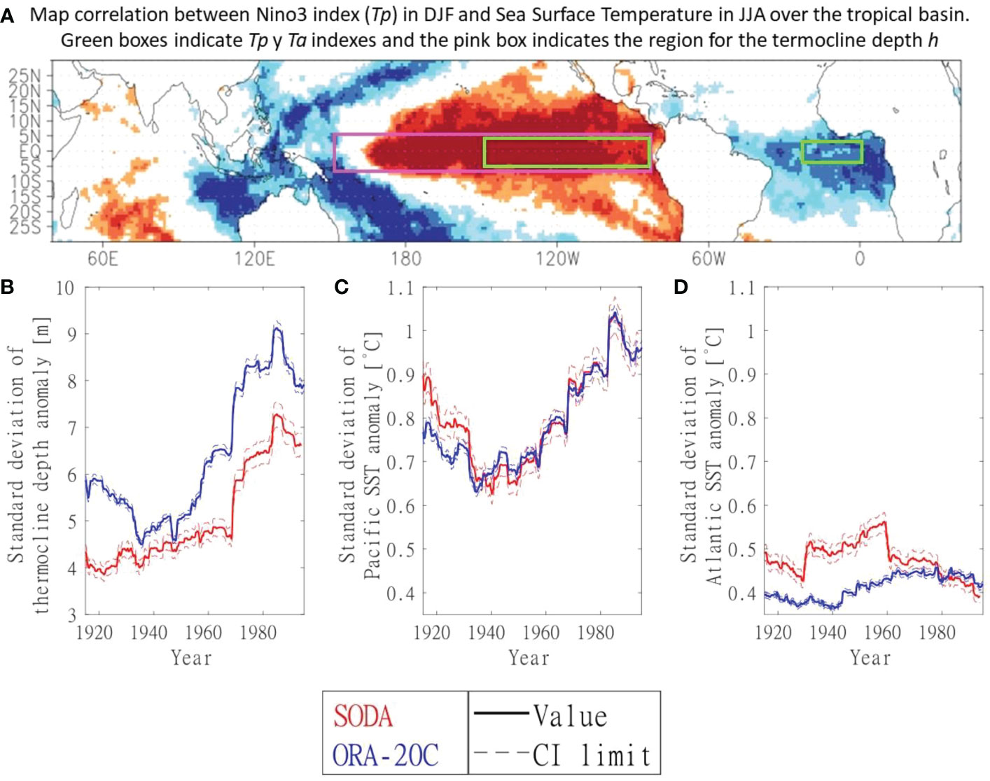
Figure 1 Climate indexes: (A) Map representing the boxes for the three indexes T_P, T_A (green boxes in the Pacific and Atlantic, respectively) and h (pink box). The shaded areas represent the correlation between the Nino3 index (T_P) in DJF and SST in previous summer JJA. Red (blue) colors represent positive (negative) rank correlations. (Panels B-D) Characteristic amplitude of the indexes anomalies: Pacific thermocline depth ε_h (B), Pacific temperature ε_P (C) and Atlantic temperature ε_A (D) anomalies, calculated as the standard deviation of the anomalies in each 30-year long time window, for SODA (red) and ORA-20C (blue) reanalysis. Solid lines represent the value of the parameter, and dashed lines show the confidence intervals of the standard deviation, as calculated in Supplementary Appendix (D) Each point of the figure considers a time window of 30 years, and the represented year in the horizontal axis is the mean value of that interval.

TABLE 1

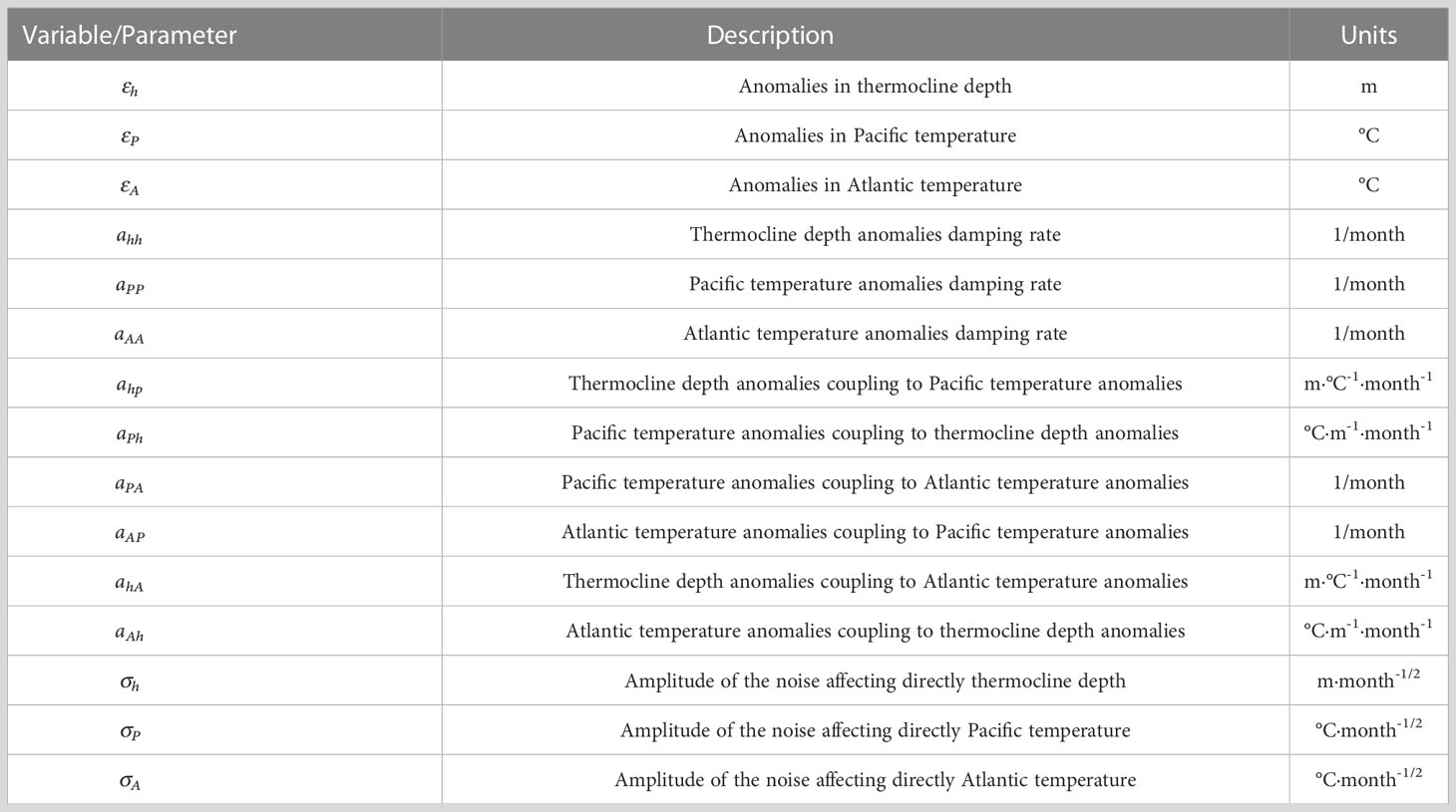
Table 1 Main variables and parameters used in this article, description and units.

The characteristic amplitude of the anomalies in temperature and thermocline depth is given by their standard deviation for each 30-year time window (see Figures 1B–D). The results obtained with the two reanalysis show an increase of both Pacific anomalies from the 40s. The magnitude of the anomalies is similar for both reanalyses, although ORA-20C gives greater values for the thermocline depth anomalies. Atlantic temperature anomalies do not present a clear increase, and both reanalysis only begin to be consistent from the 60s.

In using long oceanic datasets, a word of caution is appropriate. Reanalysis products are the result of a coupled atmosphere-ocean model run constrained to the available observations through a data assimilation procedure. At the equator, the quantity and quality of oceanic datasets increased greatly around the 1980’s, particularly after the establishment of the Tropical Ocean-Global Atmosphere (TOGA) observing system (see Yu et al., 2020). Therefore, changes in the oscillatory behavior of ENSO provided by reanalysis products in the earlier part of the century may be influenced by the different quality of the datasets used in the assimilation systems.

2.2 Models

The present study is performed in the linear framework of the recharge oscillator model to describe both the ENSO dynamics and the Pacific-Atlantic inter-basin coupling. The explicit form of the model equations is

$\begin{array}{ll}\left(\begin{array}{c}d{ϵ}_h\\ d{ϵ}_P\\ d{ϵ}_A\end{array}\right)=\left(\begin{array}{ccc}{a}_{hh}& a_{hP}& a_{hA}\\ a_{Ph}& a_{PP}& a_{PA}\\ a_{Ah}& a_{AP}& a_{AA}\end{array}\right)\left(\begin{array}{c}{ϵ}_h\\ {ϵ}_P\\ {ϵ}_A\end{array}\right)dt+\left(\begin{array}{c}{\sigma }_{h}d{B}_h\\ {\sigma }_{P}d{B}_P\\ {\sigma }_{A}d{B}_A\end{array}\right),& (1)\end{array}$

where ε_h are the anomalies in Pacific thermocline depth, ε_P are the anomalies in the Pacific Ocean SST, and ε_A are the anomalies in the Atlantic Ocean SST, in the regions indicated in Figure 1. The traditional recharge oscillator model (Jin, 1997) only has ε_P and ε_h as prognostic variables. The model solution can be written as (2) with ε₁=ε_h, ε₂=ε_P, and ε₃=ε_A, and the matrix A obtained by fitting to the data, as described in the following subsection.

From the matrix coefficients a_jk, we can compute the oscillation period and the decay (damping) time. To have an oscillatory behavior, the matrix of coefficients must have a pair of complex conjugate eigenvalues (oscillation condition), as is the case with ENSO. Oscillations become more apparent as the oscillation period increases with respect to the decay time (as we will see has happened during the last decades).

2.3 Fitting methods

Our models can be synthesized as three time series of anomalies ε_j, j=1,2,3 that satisfy the following relationships,

$\begin{array}{ll}\frac{d{ϵ}_j}{dt}={\displaystyle \sum _{k=1}^N{a}_{jk}{ϵ}_k+{\xi }_j.}& (2)\end{array}$

The deterministic part of the time derivative of the anomalies in Eq. 2 is linear on their amplitudes with coefficients a_jk, forming the matrix A. The diagonal coefficients a_jj give the damping rates of the anomalies, i.e., how fast the anomaly decreases (in the absence of other contributions). The non-diagonal coefficients a_jk give the couplings between the anomalies, i.e., how much each anomaly is affected by each of the others. The stochastic (= non-deterministic) term, ξ_j, is assumed to be a Gaussian white noise (for time scales larger than 3 days). As the stochastic term ξ_j is a Gaussian white noise, Eq. 2 is equivalent to

$\begin{array}{ll}d{ϵ}_j={\displaystyle \sum _{k=1}^N{a}_{jk}{ϵ}_{k}dt+{\sigma }_{j}d{B}_j,}& (3)\end{array}$

where dB_j is the derivative of a Wiener Process (with 〈dB_j(t)dB_k(t+t^′)〉={dt δ_jk, for  t^′=0; 0, for  t^′≠0 ) and σ_j is the amplitude of the noise affecting each anomaly directly. We next review methods used to obtain the matrix A in Eq. 3 in order to reproduce the correlation functions of the anomalies ε_j, j=1,2,3 with time series of data for a period 0<t<T. First, we define the correlation of the anomalies as

$\begin{array}{ll}{c}_{jk}\left(t_0\right)=<{ϵ}_j\left(t\right){ϵ}_k\left(t_0+t\right)>& (4)\end{array}$

For each time window, we numerically calculate the autocorrelations (j = k) and cross-correlations (j ≠ k) of the normalized anomalies. Next, we search for the set of coefficients a_jk that gives the best fit of the Fisher’s Z transform for the correlation functions $c_{jk}^N\left(t,A,{\sigma }_1,{\sigma }_2\right)$, to the data correlation functions minimizing the square error up to a maximum lag |t_max|=36 months (i.e., in a time interval less than or equal to three years), and considering the uncertainty in each point to weight the fitting. (Further details in Supplementary Information: Appendixes A, B, and D).

3 The recharge oscillator model with the ReOsc and ReOsc+ methods

The traditional fitting of the recharge oscillator model (ReOsc; Vijayeta and Dommenget, 2018; Crespo et al., 2022) consists of a mean squares minimization fit of the discretized version of Eq. 2 for two-variables (N = 2), neglecting the stochastic term,

$\begin{array}{ll}\Delta \overrightarrow{{ϵ}_j}={\displaystyle \sum _{k=1}^2{a}_{jk}\overrightarrow{{ϵ}_k}\Delta t,}& (5)\end{array}$

where $\overrightarrow{{ϵ}_k}$ are vectors containing the anomalies on each time step in a selected period (30-year windows in our case), the anomaly change per time step, $\Delta \overrightarrow{{ϵ}_j}$, is defined by $\Delta \overrightarrow{{ϵ}_j}\left(t_l\right)=\overrightarrow{{ϵ}_j}\left(t_l+\Delta t\right)-\overrightarrow{{ϵ}_j}\left(t_l\right)$, and Δt is the duration of the time step, which is chosen as the time lapse between two consecutive measures in the reanalysis (1 month).

Thus, the residuals on each time step are equal to ξ_j(t_l)Δt, and we can obtain σ_j by calculating their standard deviation:

${\xi }_{j}dt={\sigma }_{j}d{B}_j\to \langle {\xi }_j\left(t\right){\xi }_j\left(t\right)d{t}^2\rangle = {\sigma }_j^2<d{B}_j\left(t\right)d{B}_j\left(t\right)>\to$

$\begin{array}{ll}var\left(Re{s}_j\right)={\sigma }_j^2\Delta t\to {\sigma }_j=\frac{std\left(Re{s}_j\right)}{\sqrt{\Delta t}},& (6)\end{array}$

where <> means expected value. This method tends to minimize the residuals and consequently to minimize the amplitudes of the noises in the model.

Recall we refer to the fitting described above in this section as ReOsc and to the fitting method described in Section 2.3 as ReOsc+.

Figure 2 shows the data cross-correlation functions compared with the model cross-correlation functions given by the ReOsc and ReOsc+ methods for the traditional recharge oscillator model of ENSO with two variables in the equatorial Pacific. (The analytic expressions of the model auto and cross-correlations are shown in Supplementary Appendix E). The periods of analysis are the same as those in Crespo et al. (2022), where ENSO evolution was studied using the ReOsc method. The new fitting method, ReOsc+, gives model correlations functions that fit better than those with the reanalysis data for both SODA and ORA-20C. This new fitting also gives smaller uncertainties and smoother evolutions for the characteristic damping and oscillation times. See Supplementary Appendix A. The results obtained agree with Crespo et al. (2022) in that ENSO evolution is more closely described by the model from the 1970s, having the anomalies of the equatorial heat content a strong impact on the SST anomalies with ten months lead.

FIGURE 2

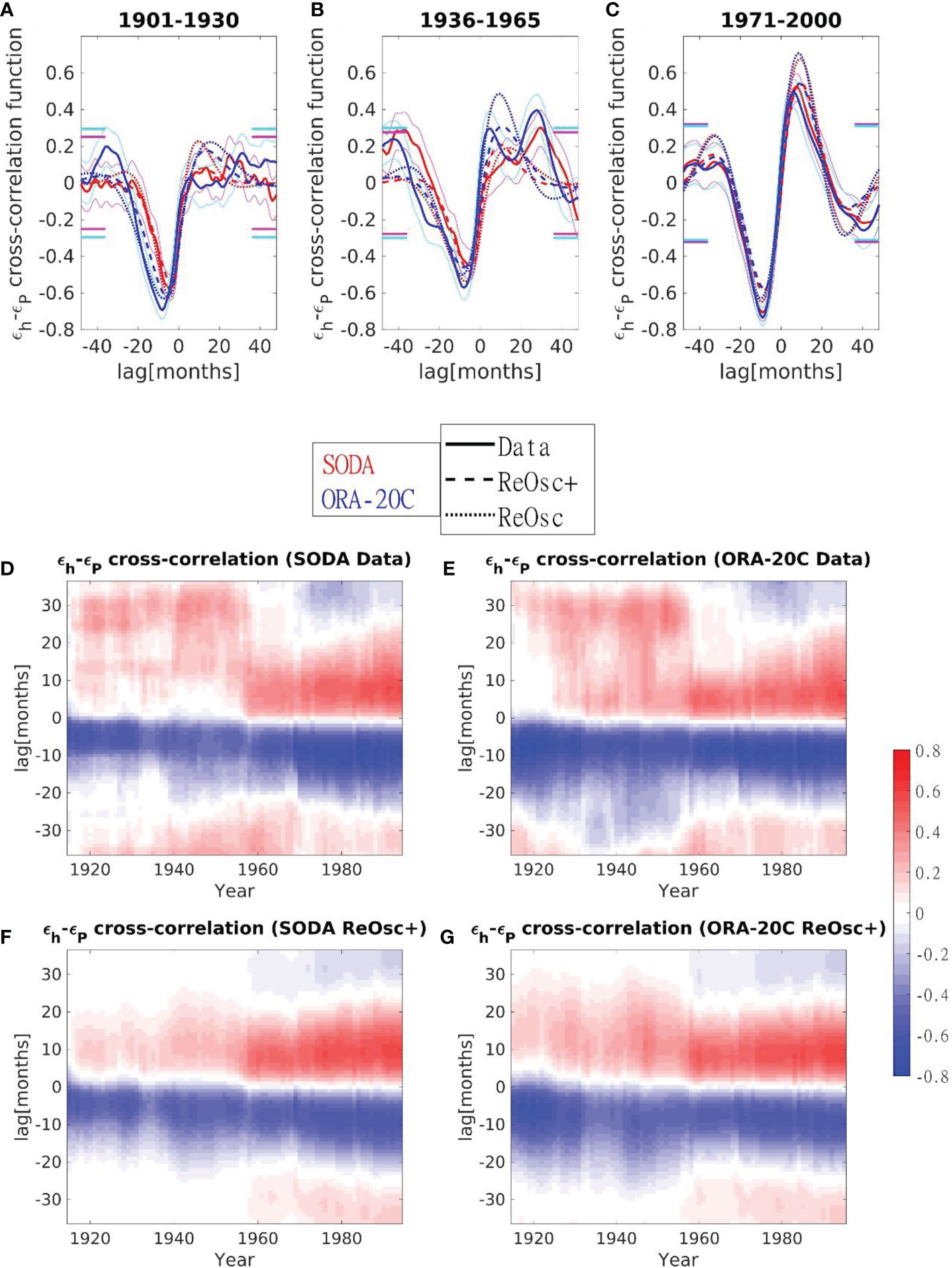
Figure 2 Normalized cross-correlation functions. $c_{hP}^N$, between the Pacific thermocline depth and the Pacific SST anomalies for the periods 1901-1930 (A), 1936-1965 (B), and 1971-2000 (C), SODA (solid red line) and ORA-20C (solid blue line, mean of all members) data, ReOsc+ model (dashed line) and ReOsc model (dotted line) for the two-variable Pacific-Atlantic dynamics (Eq. 7 fitted as explained in Section 2.3). Magenta (for SODA) and cyan (for ORA-20C) thin lines show the 95% confidence interval of the data crosscorrelation (see Supplementary Appendixes A, D). Magenta (for SODA) and cyan (mean of all members for ORA-20C) thick lines show the uncertainty in uncorrelation beyond 36 months, i.e., solid lines inside those limits indicate that there are no significant contributions from the correlations beyond 36 months (see Supplementary Appendix B). (D–G) Color map of the normalized cross-correlation function for SODA (period 1900-2008) and ORA-20C (period 1900-2009, mean of all members) reanalysis, both for the data (D, E, respectively) and for the ReOsc+ model (F, G, respectively). Each column represents the function for a time window of 30 years, and the represented year in the horizontal axis is the mean value of that interval. The vertical axis indicates the lag in the cross-correlation function (if positive, h leads). Red Blue Colormap (Auton, 2022) was used in Panels (D–G) of this figure.

The oscillation period and decay time have simple expressions for the two-variable recharge oscillator model, in which A is a 2x2 matrix. If the eigenvalues of A are complex (see Supplementary Appendix C), the oscillation period is given by the expression $t_o=\frac{4\pi }{\sqrt{4D-T{r}^2}}$, where D is the determinant of the matrix of coefficients; D=a_PPa_AA−a_PAa_AP, and T_r is the trace of the matrix of rates of coefficients; Tr=a_PP+a_AA. When eigenvalues are complex, the decay (damping) time is given by the expression $t_d=\frac{-2}{Tr}$. For real eigenvalues, we represent $\overline{t_d}=\frac{-2}{Tr}$ as an estimate of the mean value, and we use t_d,1+Δ_td,1, and t_d,2+Δ_td,2 as estimates of the confidence interval limits, where $t_{d,1,2}=\frac{-2}{Tr\mp \sqrt{T{r}^2-D}}$ and Δt_d,1,2 are their uncertainties as explained in Supplementary Appendix D.

In the following, we analyze the evolution of the Pacific temperature and thermocline depth anomalies, ε_P and ε_h during the last century. For this, we examine the cross-correlation functions for different time windows in the period we are analyzing (Figure 2). For SODA data, a single cross-correlation is calculated for each time window, while for ORA-20C data, the value plotted is the average of those calculated for the five-members ensemble (see Supplementary Appendix D).

For both reanalyses, the maximum (red in panels D-E of Figure 2) is more pronounced in recent times, which means a more significant effect of thermocline depth anomalies ε_h on temperature anomalies ε_P during the period. The maximum of the crosscorrelation c_hP(t₀)=〈ϵ_h(t)ϵ_P(t₀+t)〉  for positive lags means that in the Pacific, positive anomalies in thermocline depth are followed by positive anomalies in temperature, i.e., that we can expect that such anomalies in thermocline depth are followed by a Niño (Niña) event in the Pacific Ocean 8 months later (Panels A-E of Figure 2). The minimum of the cross-correlation (blue in Panels D-E of Figure ε_P) remained nearly constant during the last century. This minimum for negative lags indicates the negative effect of temperature anomalies on future thermocline anomalies. The simultaneous presence of both these maximum and this minimum features is a hallmark of the presence of oscillations, as we see below.

A deeper insight into the coupled dynamics of the Pacific thermocline depth anomaly and the Pacific SST can be obtained by fitting the dynamics to the recharge oscillator model.

$\begin{array}{ll}\left(\begin{array}{c}d{ϵ}_h\\ d{ϵ}_P\end{array}\right)=\left(\begin{array}{cc}{a}_{hh}& a_{hP}\\ a_{Ph}& a_{PP}\end{array}\right) \left(\begin{array}{c}{ϵ}_h\\ {ϵ}_P\end{array}\right)dt+\left(\begin{array}{c}{\sigma }_{h}d{B}_h\\ {\sigma }_{P}d{B}_P\end{array}\right) , & (7)\end{array}$

The parameters of the recharge oscillator model are the damping rates (a_ii, diagonal elements of the A matrix), the couplings (a_jk, off-diagonal elements of the A matrix) and the noise amplitudes affecting each anomaly, σ_j. Here, we obtain the parameter values using the ReOsc+ approach. (For details on the procedure, see Section 2.4 and Supplementary Appendix A.) The correlation functions obtained with the ReOsc+ model show a good agreement with the data for lags of less than 20 months, see Figure 2.

The absolute value of the damping rate of thermocline depth anomalies, a_hh, decreased throughout the 20^th century (see panel A of Figure 3). This means that the thermocline depth anomalies have been more persistent in recent years. The damping rate of the Pacific temperature a_PP experienced great variations before the 1950s and stabilized around 0.07 months^-1. Off-diagonal elements of the matrix of coefficients, a_hP and a_Ph, show higher variability, and the values depend more on the reanalysis. Regarding the noises, the one affecting thermocline depth has not varied significantly (in mean) over the 20^th century, except for a sudden increase around the 1970s (Figure 3). Conversely, the noise amplitude on Pacific temperatures decreased until the 1950s and after increased. Mean parameters uncertainties are about 10% in SODA and 5% in ORA-20C (See Figure 3, and Table D1 in Supplementary Appendix D).

FIGURE 3

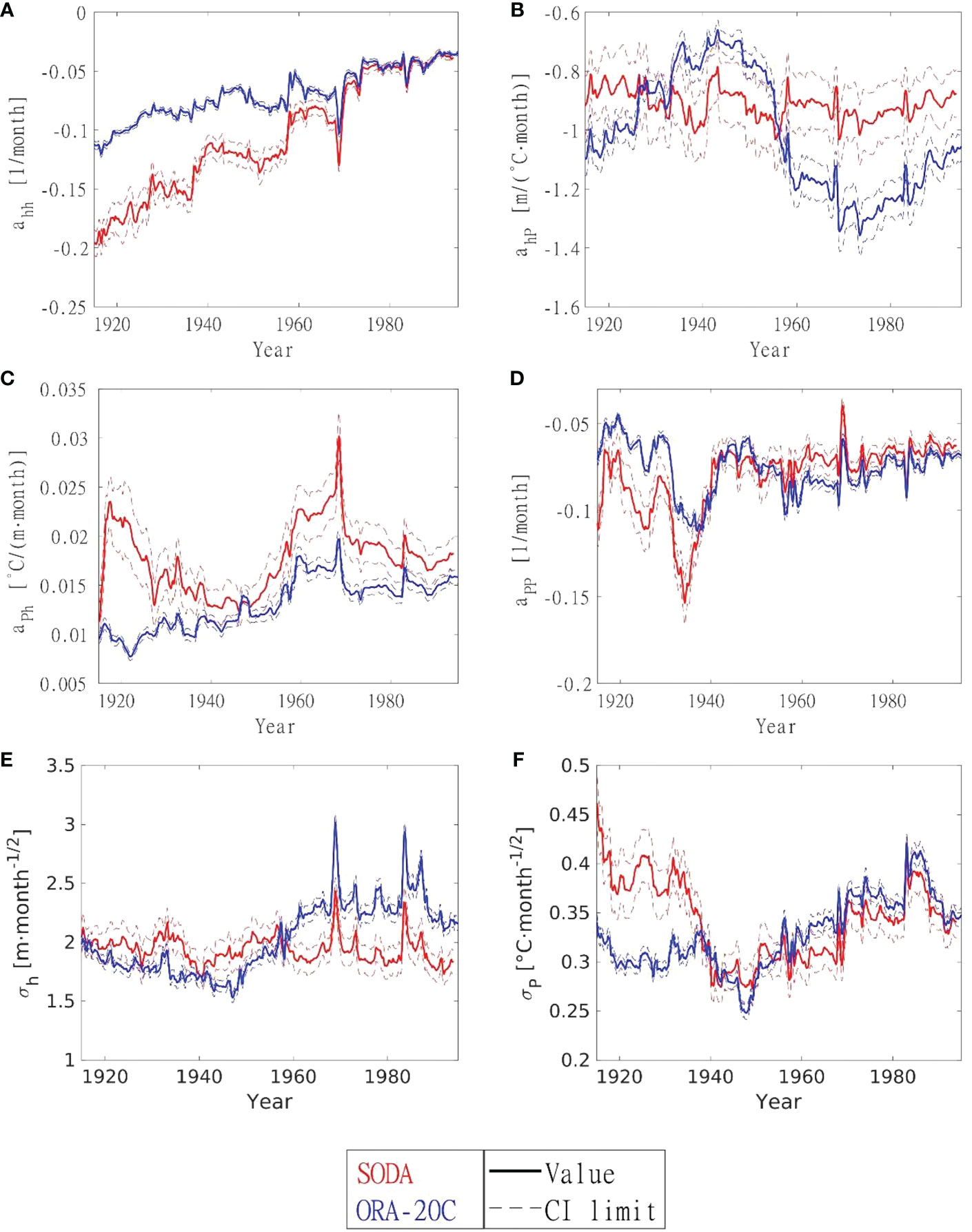
Figure 3 Parameter evolution computed with the ReOsc+ model for ENSO (Eq. 7 fitted as explained in Section 2.3): Damping rates (a_hh and a_PP), couplings (a_hP and a_Ph) and noise amplitudes (σ_h and σ_P) in the period 1900-2009 for SODA (red) and ORA-20C (blue) reanalysis. (A) Damping rate of the anomalies in Pacific thermocline depth (a_hh). (B) Coupling of the Pacific thermocline depth to Pacific SST (a_hP). (C) Coupling of Pacific SST to the Pacific thermocline depth (a_Ph). (D) Damping rate of the anomalies in Pacific SST (a_PP). (E) Noise amplitude directly affecting Pacific thermocline depth anomalies. (F) Noise amplitude directly affecting Pacific SST anomalies. Each point of the figure considers a time window of 30 years, and the represented year in the horizontal axis is the mean value of that interval. Solid lines represent the parameter’s values, and dashed lines show the (1-standard-deviation) confidence intervals (Supplementary Appendix D).

To gain insight into the relative importance of the parameters, we make that all terms in the matrix of coefficients a_jk have units of month^-1 through multiplying each a_jk by the typical size of the fluctuations by the typical size of the fluctuations S_k (units of [ε_k]) and divide by S_j (units of [ε_j]), i.e., $\widetilde{a_{jk}}=a_{jk}·\frac{S_k}{S_j}$. The results are shown in the fifth and sixth rows of Table 2. Table 2 shows that couplings in both directions have similar magnitudes. This indicates that the differences between the two first rows of Table 2, were because the typical amplitude of thermocline depth (in meters) is several times greater than the typical variations in temperature (in °C), as shown in the fourth row of Table 2.

TABLE 2

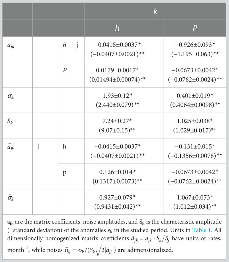
Table 2 Parameters (and 1-standard-deviation confidence intervals) obtained by the fitting with the two-variable ReOsc+ ENSO model (Eq. 7 fitted as explained in Section 2.4) for SODA (marked with *) and ORA-20C (with parenthesis, marked with **) reanalysis in the 1971-2000 period.

Analogously we can non-dimensionalize the noise amplitude σ_j, dividing it by the typical size of this fluctuation S_j (units of [ε_j]), and by the square root of the characteristic damping of these fluctuations, $\sqrt{\left|a_{jj}\right|}$ (with units of month^-1/2). This procedure gives the adimensionalized noise amplitude ${\tilde{\sigma }}_j=\frac{{\sigma }_j}{S_j\sqrt{2\left|{\tilde{a}}_{jj}\right|}}$, where the additional division by $\sqrt{2}$ makes that it gives 1 in the uncoupled case. The non-dimensionalized noises ${\tilde{\sigma }}_j$ are given in the third column of Table 2, which shows that the noise contributions to each of the anomalies are of the same order.

The decay (damping) time is the characteristic time of decrease of a fluctuation (i.e., when it has decreased a factor e^-1). This quantity has increased (for both reanalyses) through the 20th century, see Figure 4. The oscillation period measures the time required to complete a full oscillation. It has mildly decreased (for both reanalyses) through the 20th century, see Figure 4. Note that for the last decades, decay and oscillation times have a similar order of magnitude (a few years), implying more marked oscillations in ENSO.

FIGURE 4

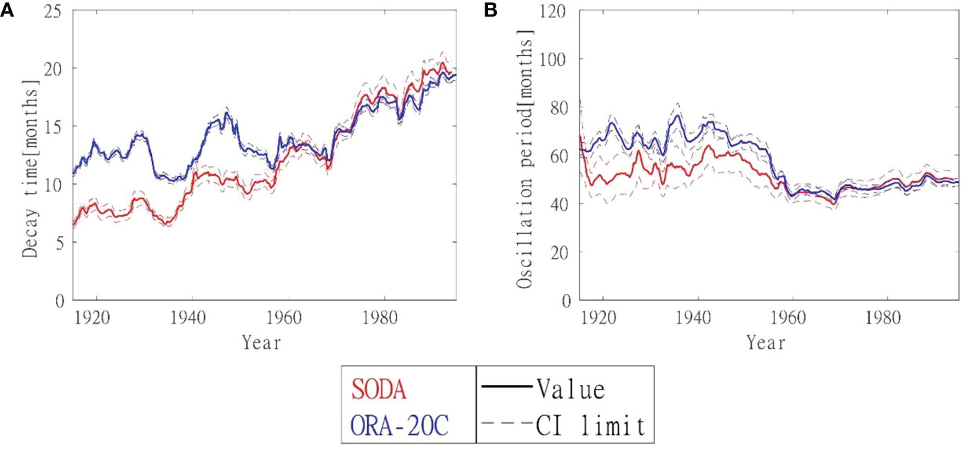
Figure 4 Decay times (A) and oscillation period (B) for the ReOsc+ model for ENSO (Eq. 7 fitted as explained in Section 2.3) in the period 1900-2009 for SODA (red) and ORA-20C (blue) reanalysis. Each point of the figure considers a time window of 30 years, and the represented year in the horizontal axis is the mean value of that interval. Solid lines represent the value of the characteristic times, and dashed lines show the (1-standard-deviation) confidence intervals. (They were computed as described in Section 3 and Supplementary Appendix D, respectively).

We recall that these results have been obtained with the ReOsc+ method. The ReOsc method gives higher uncertainties and does not allow us to estimate the oscillation period before the 60s (see Figure A2 in Supplementary Appendix A).

4 Covariability between equatorial Pacific and Atlantic SSTs in the SODA and ORA-20C reanalysis

As stated in the Introduction, the Atlantic and Pacific equatorial SST anomalies appear highly correlated from the 1970’s (Rodríguez-Fonseca et al., 2009). To study this interbasin SST coupling in other periods, we can apply the two variables model and our new fitting methodology (ReOsc+) again. The mathematical approach is analogous to the one adopted in the previous section, and to simplify, we will also call it ReOsc+ model. However, the physical meaning of the model and its coefficients is different as it couples SST anomalies in two different regions (instead of the SST anomalies and thermocline depth anomaly in the same region). This approach addresses the issue of the relationships between the equatorial Atlantic and Pacific, which are still under debate because they depend upon the period of study (Rodríguez-Fonseca et al., 2009; Martín-Rey et al., 2014; Martín-Rey et al., 2015; Mechoso, 2020). Starting from the observations of the temperature anomalies, ε_A and ε_P, in both the Pacific and Atlantic oceans (for the period from 1900 to 2009), the ReOsc+ gives the matrix coefficients, a_jk, and the amplitudes of the noise affecting each anomaly, σ_j (further details in section 2.3, and in Appendix A of the Supplementary Information).

Therefore, we calculate the cross-correlation function among these indexes and fit the parameters of the model with ReOsc+ method explained in section 2.3 (and Supplementary Appendix A). Figure 5 shows that correlation functions before the 1960s (approximately) are very irregular, suggesting that a real coupling between both oceans may be either very weak or even absent before this period. For both reanalyses, maxima and minima are much smaller than those found for the Pacific ENSO (compare Figures 2, 5).

FIGURE 5

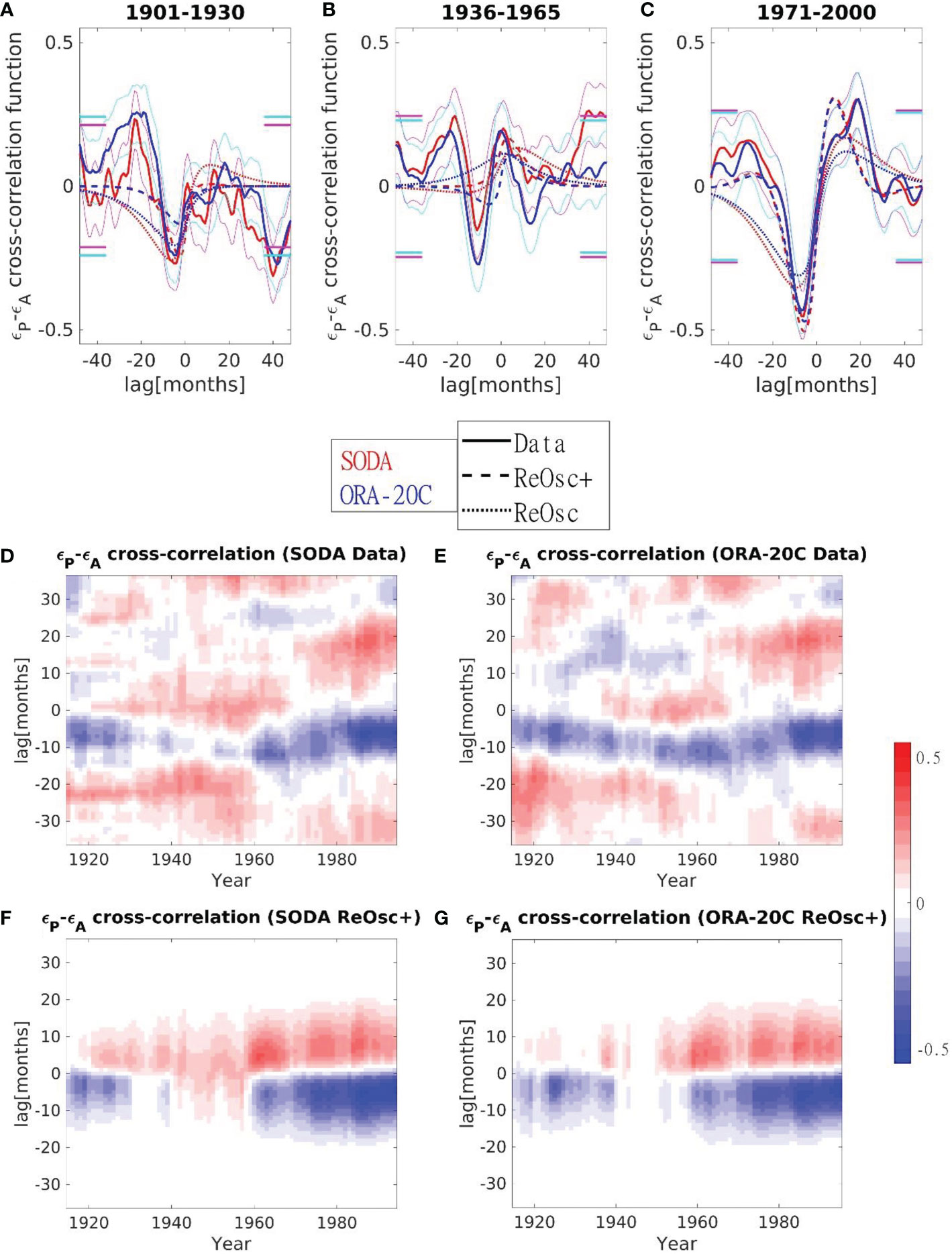
Figure 5 Normalized cross-correlation functions, $c_{PA}^N$, between the Pacific SST and the Atlantic SST anomalies for the periods 1901-1930 (A), 1936-1965 (B), and 1971-2000 (C), represented for SODA (solid red line) and ORA-20C (solid blue line, mean of all members) data, ReOsc+ model (dashed line) and ReOsc model (dotted line) for the two-variable Pacific-Atlantic dynamics (Eq. 8 fitted as explained in Section 2.3). Magenta (for SODA) and cyan (for ORA-20C) thin lines show the 95% confidence interval of the data crosscorrelation (see Supplementary Appendixes A, D). Magenta (for SODA) and cyan (mean of all members for ORA-20C) thick lines show the uncertainty in correlation beyond 36 months, i.e., solid lines inside those limits indicate that there are no significant contributions from the correlations beyond 36 months (see Supplementary Appendix B). (D–G) Color map of the normalized cross-correlation function for SODA (period 1900-2008) and ORA-20C (period 1900-2009, mean of all members) reanalysis, both for the data (D, E, respectively) and for the ReOsc+ model (F, G, respectively). Each column represents the function for a time window of 30 years, and the represented year in the horizontal axis is the mean value of that interval. The vertical axis indicates the lag in the cross-correlation function (if positive, Pacific leads). Red Blue Colormap (Auton, 2022) was used in (D–G) of this figure.

Now we proceed to fit the interaction between the Atlantic and Pacific variability using the two variables model (ReOsc+ model),

$\begin{array}{ll}\left(\begin{array}{c}d{ϵ}_P\\ d{ϵ}_A\end{array}\right)=\left(\begin{array}{cc}{a}_{PP}& a_{PA}\\ a_{AP}& a_{AA}\end{array}\right)\left(\begin{array}{c}{ϵ}_P\\ {ϵ}_A\end{array}\right)dt+\left(\begin{array}{c}{\sigma }_{P}d{B}_P\\ {\sigma }_{A}d{B}_A \end{array}\right) , & (8)\end{array}$

Note that before the 1960s, for some time windows, the fitting gives non-oscillating correlation functions, with only negative or positive cross-correlations (Figure 5). Since the 60s, most significant maxima are found for positive lags and minima for negative lags, both for data and ReOsc+ model. However, the positive maxima are shifted in the ReOsc+ compared with observations (6 months vs. 20 months), while the negative minima are coherent in ReOsc+ and observations after the 1960s. This negative correlation implies that Atlantic Niño (Niña) leads the Pacific Niña (Niño) by 6 months.

The absolute value of the damping rate (diagonal elements) of both temperature anomalies decreases, implying slower damping rates and an increase in the overall decay time (see Figures 6, 7). The absolute values of coupling rates (off-diagonal elements) show an overall increase in the analysis period. These results point towards an enhancement in time of the coupling leading to an oscillatory behavior for these coupled temperatures, which becomes more apparent after the 60s, as is better shown in Figure 7. The other parameters obtained with the ReOsc+ model are the noise amplitudes affecting each anomaly, σ_j. Figure 6 shows a large time variability of the Pacific temperature noise, and a reanalysis dependent decrease in the Atlantic temperature noise. The parameters’ uncertainties are generally much greater than those obtained for Pacific ENSO, due to their low correlation (low Atlantic-Pacific interaction), particularly before the 1960s (see Table D2 in Supplementary Appendix D).

FIGURE 6

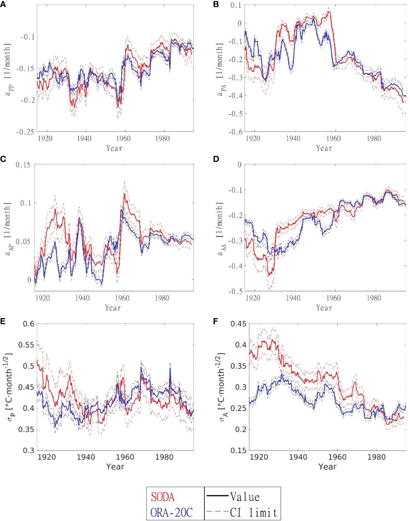
Figure 6 Parameter evolution computed with the ReOsc+ model for Atlantic-Pacific SST system (Eq. 8 fitted as explained in Section 2.3): Damping rates (a_PP and a_AA), couplings (a_PA and a_AP) and noise amplitudes (σ_P and σ_A) in the period 1900-2008 for SODA (red) and in the period 1900-2009 for ORA-20C (blue) reanalysis. (A) Damping rate of the Pacific SST anomaly (a_PP). (B) Coupling of the Pacific to the Atlantic SST anomalies (a_PA). (C) Coupling of the Atlantic to the Pacific SST anomalies (a_AP). (D) Damping rate of the Atlantic SST anomaly (a_AA). (E) Noise amplitude directly affecting the Pacific SST anomaly. (F) Noise amplitude directly affecting the Atlantic SST anomaly. Each point of the figure considers a time window of 30 years, and the represented year in the horizontal axis is the mean value of that interval. Solid lines represent the parameter’s value, and dashed lines show the (1-standard-deviation) confidence intervals (Supplementary Appendix D).

FIGURE 7

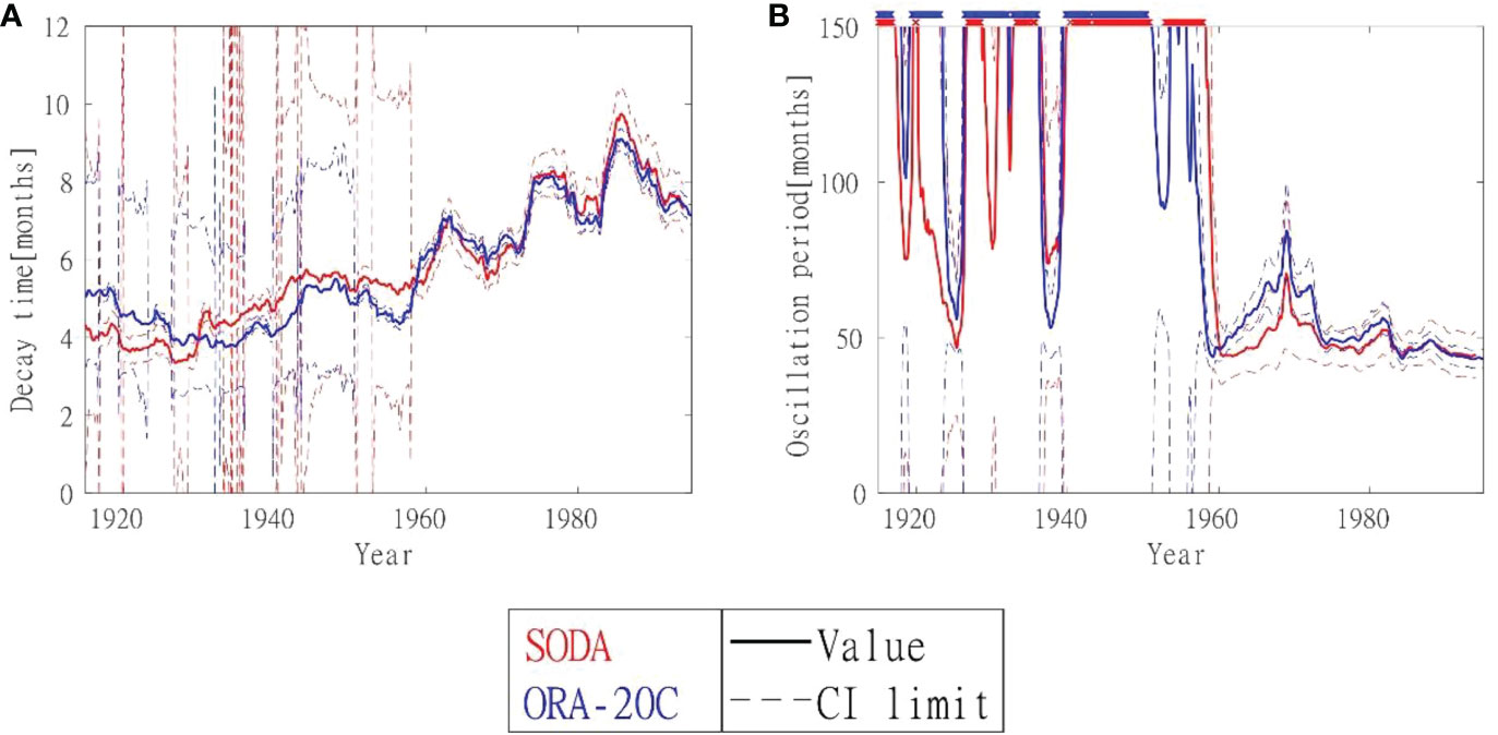
Figure 7 Decay times (A) and oscillation period (B) for the ReOsc+ model for the Atlantic-Pacific SST system (Eq. 8 fitted as explained in Section 2.3) in the period 1900-2008 for SODA (red) and in the period 1900-2009 for ORA-20C(blue) reanalysis. Each point of the figure considers a time window of 30 years, and the represented year in the horizontal axis is the mean value of that interval. Solid lines represent the value of the characteristic times, and dashed lines show the (1-standard-deviation) confidence intervals. (They were computed as described in Section 3 and Supplementary Appendix D, respectively). In the right panel (red for SODA and blue for ORA-20C), crosses denote windows with a non-oscillating regime (i.e., we cannot represent oscillation periods).

We computed the oscillation period and the decay time as described in Section 3, see Figure 7. Before the 60s, we found very long oscillation periods with huge uncertainties or even non-oscillating regimes (eigenvalues are real) for some time windows. After the 60s, oscillation periods have typical values between 50 and 100 months. Decay time has mildly increased (for both reanalyses) through the 20th century and is much shorter than the decay time found for Pacific ENSO. The periods with real eigenvalues that appear before the 60s present larger uncertainties in the decay time.

To get further insight into the coupled dynamics after the 60s we show in Table 3 the fitted parameters for the period 1971-2000. Additionally, Table 3 shows the dimensionally homogenized parameters (as previously described in Section 3). Table 3 shows that couplings in both directions have similar magnitudes. The couplings are weaker than for ENSO. This weaker coupling supports the need for a three-variable model, including ENSO coupling and Pacific-Atlantic SST coupling, which will be presented in the next section.

TABLE 3

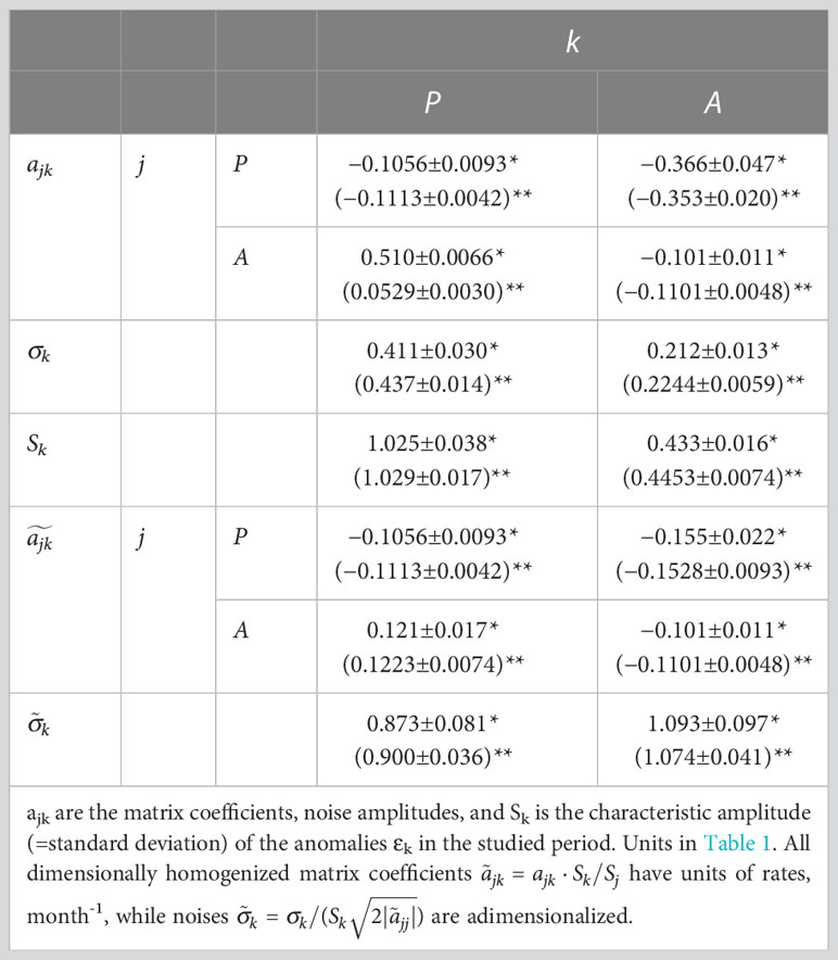
Table 3 Parameters (and 1-standard-deviation confidence intervals) obtained by the fitting with the two-variable ReOsc+ Atlantic-Pacific model (Eq. 8 fitted as explained in Section 2.3) for SODA (marked with *) and ORA-20C (with parenthesis, marked with **) reanalysis in the 1971-2000 period.

5 Connecting equatorial SST and thermocline depth in the Pacific (ENSO) with equatorial Atlantic SST using the extended recharge oscillator model

In this section, we investigate the relationships between the three key variables in the extended recharge oscillator model: thermocline depth anomaly in the Pacific Ocean ε_h, and temperatures in Pacific and Atlantic Oceans, ε_P and ε_A, respectively. The non-negligible crosscorrelation between all three variables, see Figures 8, 9, motivate us to introduce a model with all three variables coupled. Additionally, the three-variable model proposed here couples the thermocline depth anomaly in the Pacific Ocean ε_h, and temperature anomalies in Pacific and Atlantic Oceans, ε_P and ε_A respectively. Figures 8, 9 show that ε_h−ε_P cross-correlations are dominant. However, there are also relevant ε_P−ε_A cross-correlations after the 60s, and even T_A−h cross-correlations. The interpretation of these 2 latter cross-correlations could give us some important clues for the Atlantic-Pacific interbasin connections.

FIGURE 8

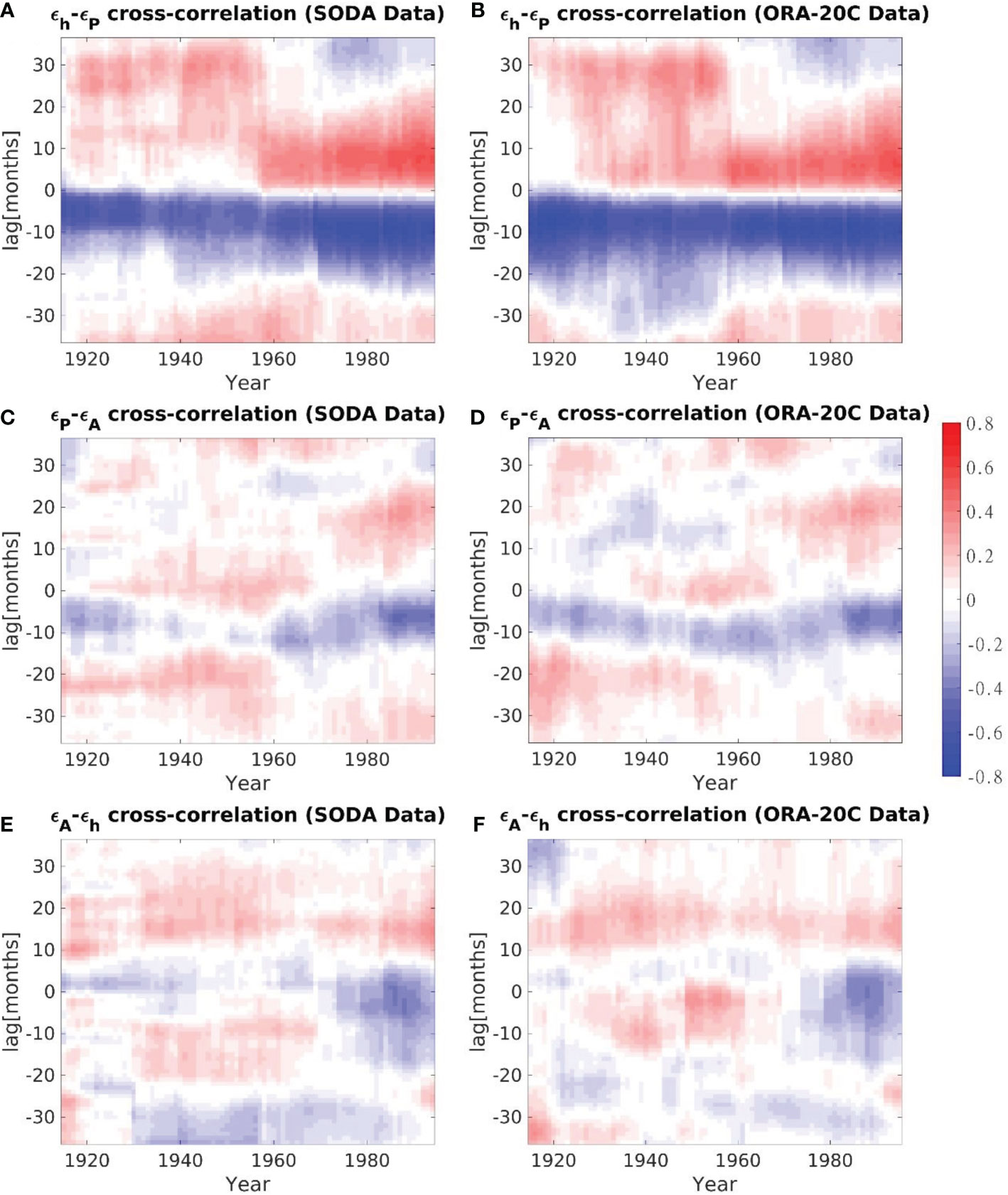
Figure 8 Color map of the normalized cross-correlation function $c_{hP}^N$ (ε_h leads for positive lags), $c_{PA}^N$ (ε_P leads for positive lags), and $c_{Ah}^N$(ε_A leads for positive lags), both for SODA (period 1900-2008, A, C, E, respectively) and ORA-20C (period 1900-2009, B, D, F, respectively) reanalysis. Each column represents the function for a time window of 30 years, and the represented year in the horizontal axis is the mean value of that interval. The vertical axis indicates the lag in the cross-correlation function. Red Blue Colormap (Auton, 2022) was used in this figure.

FIGURE 9

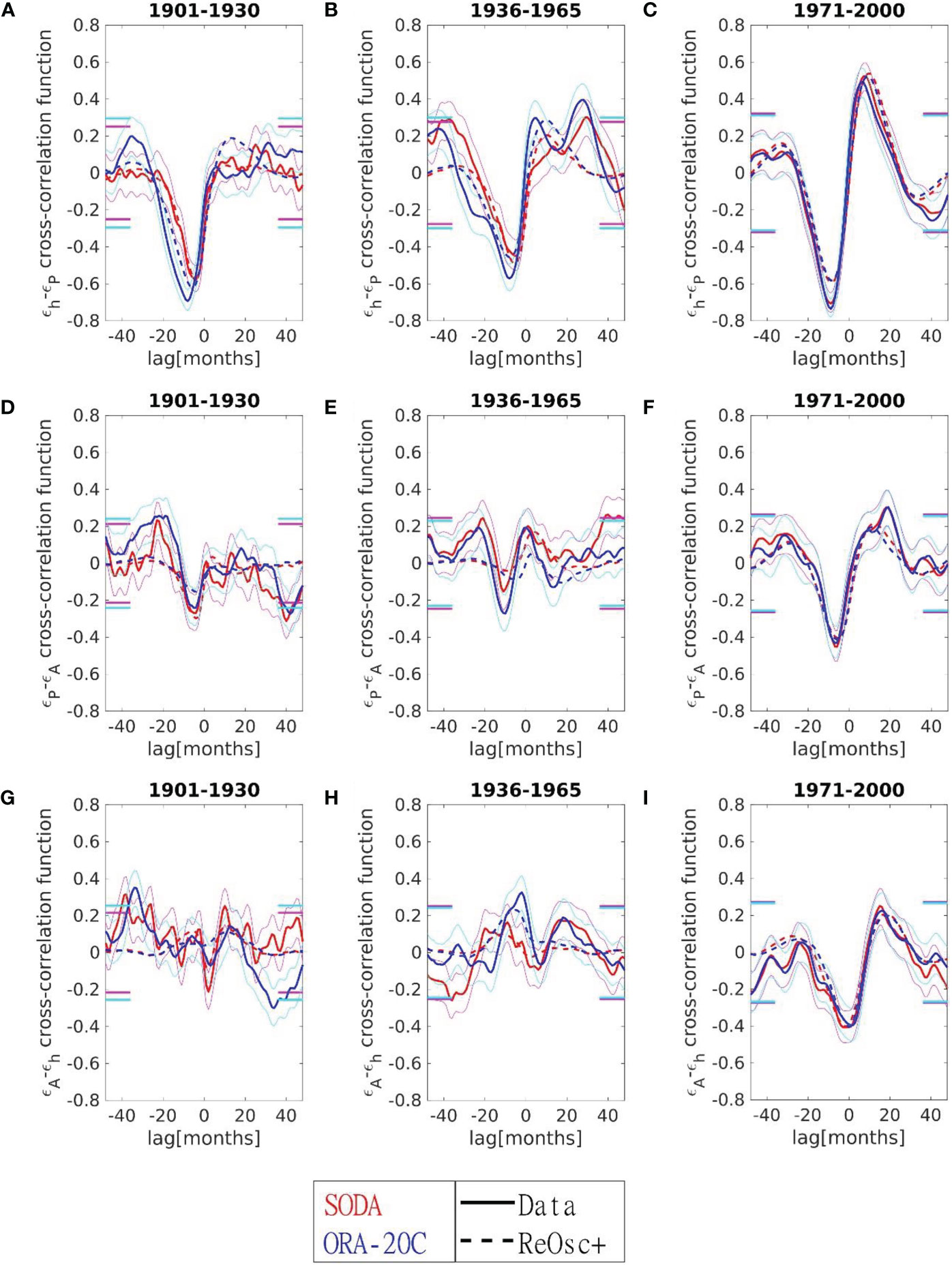
Figure 9 Normalized cross-correlation functions $c_{hP}^N$ (for the periods 1901-1930 (A), 1936-1965 (B), and 1971-2000 (C)), $c_{PA}^N$ (for the periods 1901-1930 (D), 1936-1965 (E), and 1971-2000 (F)), and $c_{Ah}^N$ (for the periods 1901-1930 (G), 1936-1965 (H), and 1971-2000 (I)), both for SODA (solid red line) and ORA-20C (solid blue line, mean of all members) data, and ReOsc+ model (dashed line) for the three-variable Pacific-Atlantic dynamics (Eq. 1 fitted as explained in Section 2.3). Magenta (for SODA) and cyan (for ORA-20C) thin lines show the confidence interval of the crosscorrelation, obtained by a Fisher’s Z transform at 95% confidence (see Supplementary Appendixes A, D). Magenta (for SODA) and cyan (mean of all members for ORA-20C) thick lines show the uncertainty in uncorrelation beyond 36 months, i.e., solid lines inside those limits indicate that there are no significant contributions from the correlations beyond 36 months (see Supplementary Appendix B).

In Figure 8, at least after the 1960s, when the data is more reliable, ε_h and ε_A are leading ε_P by 6-8 months, with a positive and negative correlation, respectively. ε_P and ε_h are strongly coupled as seen in Section 3. As in Section 4, ε_P leads ε_A by 20 months with a positive correlation. ε_A and ε_h are negatively correlated simultaneously and ε_A leads ε_h by 14 months with a positive correlation. An interesting feature is that ε_P leads ε_h negatively from the months before Atlantic impact on ENSO (Figures 8B, F) for all the periods but, just after the 1960s, ε_h leads ε_P positively (Figure 8B), completing the whole recharge-discharge mechanism. The fact the Atlantic-Pacific relation appeared after the 1960s (Figure 8F) could be helping this enhancement of the oscillatory behavior.

The three-variable model is given by the generalized recharge oscillator model presented in Eq. 1. In this case, we do not have analytic expressions for correlation functions as we did for two variables in Supplementary Appendix E. Instead, we simulate the evolution of anomalies (Eq. 3) using the following Euler Algorithm,

$\begin{array}{ll}{ϵ}_j\left(t_{l+1}\right)={ϵ}_j\left(t_l\right)+{\displaystyle \sum _{k=1}^3{a}_{jk}{ϵ}_k\left(t_l\right)\Delta t+{\sigma }_j\zeta \left(t_l\right)\sqrt{\Delta t},}& (9)\end{array}$

where ζ(t_l) is a random Gaussian variable with zero mean and variance equal to 1. The numerical integration is carried out for a maximum time of 10,000 years, at time steps t_l+1=t_l+Δt where Δt<<1month to have fine time resolution. After the integration is completed, we calculate the correlation functions numerically (starting from equilibrium, i.e., with initial conditions ε_j (0)=0), using the last 1000 years of ε_j to make sure that we reached the stationary state. This numerical procedure to obtain the correlation functions allows us to fit the correlation functions of the data for any time window with ReOsc+ method. (See Supplementary Appendix A for further details). The ReOsc+ model gives outstanding results for the last period, 1971-2000, for which fitted parameters are shown in Table 4. (See Figure 9).

TABLE 4

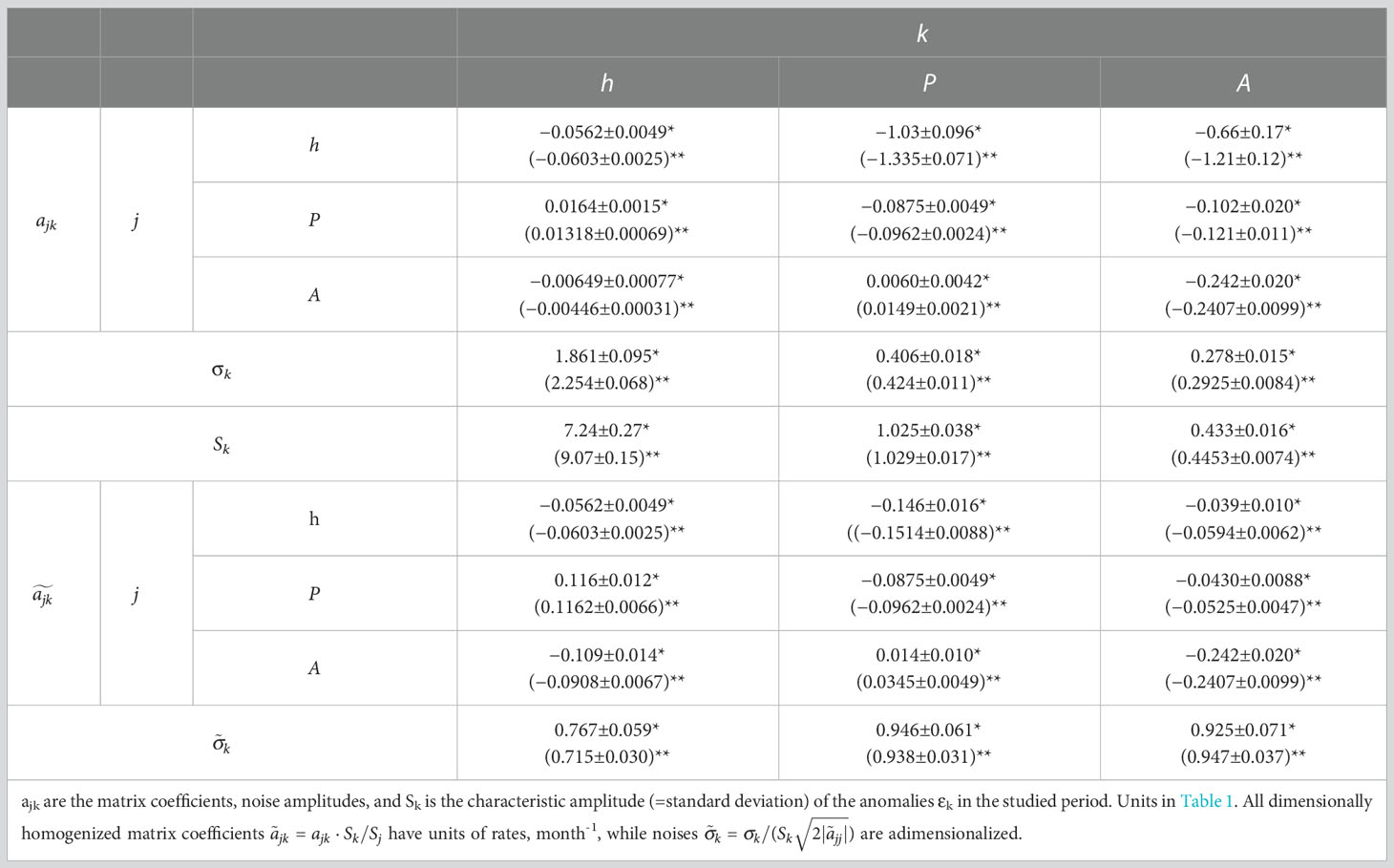
Table 4 Parameters (and 1-standard-deviation confidence intervals) obtained by the fitting with the three-variable ReOsc+ Atlantic-Pacific model (Eq. 1 fitted as explained in Section 2.3) for SODA (marked with *) and ORA-20C (with parenthesis, marked with **) reanalysis in the 1971-2000 period.

The three-variable model for the period 1971-2000 is needed to appropriately describe the Pacific-Atlantic temperature coupling (Figures 5, 9). The three-variable model gives a better fitting to the data of Pacific-Atlantic temperature anomalies (ε_P - ε_A) correlations than those obtained for two variables, and the parameters obtained by the two models show visible differences. (Compare Panel D of Figure 9 with Panel A of Figure 5, and Table 3 with Table 4.) Meanwhile, there is no significant improvement in the fitting for ENSO Pacific thermocline depth and Pacific temperature anomalies (ε_h - ε_P) correlations, and only slight differences in the parameters obtained by the two models. (Compare Panels A-C of Figure 2 with Panels A-C of Figure 9, and Table 2 with Table 4.) This result indicates that the three-variable model can improve the description of the Pacific-Atlantic temperature correlation while keeping the ENSO description’s accuracy (Pacific thermocline depth and temperature correlations).

We have also verified that imposing no coupling between the Pacific thermocline depth and Atlantic anomalies, i.e., a_hA = 0 and a_Ah = 0, leads to a significantly less accurate model [as shown using the Akaike Information Criteria (AIC) at the end of Appendix A of the Supplementary Information]. Indeed, Panel I of Figure 9 indicates how the coupling between the Pacific thermocline and Atlantic SSTs occurs at lag 0, reinforcing the idea of the role played by the Atlantic as a trigger of the Pacific Oscillator, whose impact rapidly decays. The Pacific SST is acting on the Pacific thermocline from lag -15 (Figure 9C), while the equatorial Atlantic acts on the Pacific later (Figures 9G, I), helping to develop ENSO.

Dimensionally homogenizing the parameters (${\tilde{a}}_{jk}$ in Table 4) can more accurately identify the leading couplings for the 1971-2000 period. The leading couplings are ENSO couplings (ε_P↔ε_h, in both directions), and the Pacific thermocline depth anomaly to Atlantic temperature anomaly coupling, i.e., ε_h→ε_A, as shown in Figure 10A (solid arrows). If we take into account the signs and make an ecological analogy, the ENSO coupling will appear as a predator-prey oscillatory system, also the Pacific - Atlantic coupling (as one of the coupling signs is positive while the other is negative). Conversely, the Pacific thermocline depth to Atlantic temperature coupling behaves like two competitors in this system (as the signs of both couplings are negative). These effective interactions are represented in Figure 10A with red/green arrows. They indicate, for example, that Pacific thermocline depth anomalies and Atlantic SST anomalies are “competing” to force the Pacific SST anomalies.

FIGURE 10

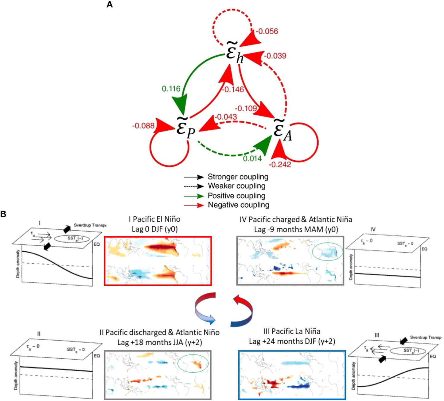
Figure 10 ENSO-Atlantic coupling. (A) Relations between Pacific thermocline depth anomaly ε_h, Pacific temperature anomaly ε_P, and Atlantic temperature anomaly ε_A found for the three-variable ENSO-Atlantic ReOsc+ model (Eq. 1 fitted as explained in Section 2.3). (A) Arrows and numbers indicate the couplings between the three variables of the model during the period 1971-2000 obtained for the SODA reanalysis, see Table 4. Tildes above epsilons indicate adimensionalization, i.e., ${\widetilde{ϵ}}_j={ϵ}_j/S_j$, where S_j is the characteristic amplitude (=standard deviation) of the anomalies ε_k The couplings are the dimensionally homogenized coupling coefficients ${\tilde{a}}_{jk}=a_{jk}·S_k/S_j$(units of month^-1). Solid arrows indicate stronger couplings and dashed arrows weaker couplings. (B) Idealized schematic of the El Niño–La Niña oscillation (modified from Jin, 1997 and Meinen and McPhaden, 2000) together with the regression maps of Nino3 index with real data for the period 1970-2000. In the schematic, thermocline depth anomaly is relative to the time mean structure along the equator. Dashed line indicates zero anomaly; shallow anomalies are above the dashed line and deep anomalies are below the dashed line. Thin arrows and symbol t represent the anomalous zonal wind stress; bold thick arrows represent the corresponding anomalous Sverdrup transports. SST is the sea surface temperature anomaly. Oscillation progresses anti-clockwise around the panels following the roman numerals; Panel I represents El Niño conditions, Panel III indicates La Niña conditions. Panel II and IV represent the phase of equatorial Pacific discharge and charge, respectively. The colored arrows represent the adjustment processes timing. The regression maps are for the SST (upper map) and OHC (lower map), which is the Ocean Heat Content integrated from surface up to 400m, representing the thermocline depth anomalies over the tropics for different lags. In the maps, red (blue) colors correspond to positive (negative) anomalies of the variables. El Niño and la Niña phases correspond to lag 0 (DJF year 0) and lag +24 months (DJF year +2), respectively. The phases of the equatorial Pacific discharge and charge correspond to lag -9 (MAM year 0) and lag +18months (JJA year +2) and appear covariant with the development of Atlantic Niña and Niño, respectively (marked with a green circle).

Figure 10B illustrates these relationships together with the traditional schematic for the Pacific Oscillator model. Therefore, positive (negative) Pacific thermocline depth anomalies, which represent a charged (discharged) Pacific, appear together with an Atlantic Niña (Niño), and this pattern is followed by Pacific El Niño (Niña) 8 months later as represented in Panel IV to I (II to III) (Figure 10B).

To get further insight into the coupling dynamics and its modes, we compute the eigenvalues and eigenvectors of the dimensionally homogenized matrix $\tilde{A}$ (with elements ${\tilde{a}}_{jk}=a_{jk}·\frac{S_k}{S_j}$, shown in Table 4; S_j is the characteristic amplitude of the anomaly ε_j given by its standard deviation). The matrix $\tilde{A}$ has three eigenvalues, which are given in the first row of Table 5. The third eigenvalue is real and determines the main damping of the system. The first two eigenvalues are complex conjugates indicating the presence of an oscillatory behavior. These eigenvalues also have a negative real part, which implies that the oscillations are damped. However, this damping is about six times weaker than the one given by the third eigenvalue.

TABLE 5

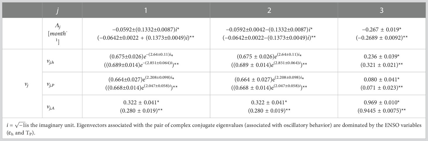
Table 5 Eigenvalues Λ_j and their respective eigenvectors v_j (1-standard-deviation confidence intervals) for the matrix of coefficients for the three-variable ENSO-Atlantic ReOsc+ model (Eq. 3 fitted as explained in Section 2.4) for SODA (marked with *) and ORA-20C (with parenthesis, marked with **) reanalysis in the 1971-2000 period.

The eigenvectors of the dimensionally homogenized matrix $\tilde{A}$ determine which are the main variables affected by oscillations and damping. The normalized eigenvector associated with the eigenvalue Λ_j is v_j = (v_j,h, v_j,P, v_j,A) and is shown in the j^th column of Table 5. (Given that eigenvectors can be multiplied by an arbitrary constant, we chose them unitary and with a real third component.) We see the real eigenvalue (which gives heavy damping) mainly influences the Atlantic Ocean because the third component (related to ε_A is the most prominent in the vector v₃. In the same way, the modulus of the third component in the vectors v₁ and v₂ is the smallest; then (damped) oscillations mainly involve the two Pacific variables (thermocline depth and temperature anomalies).

These results indicate that forcings acting mainly on the Atlantic temperature are expected to be fastly damped. Instead, forcings affecting mainly the Pacific variables may enhance the ENSO oscillations.

6 Discussion and conclusions

We have introduced a new way to fit the parameters of the recharge oscillator model to data, which consists of directly fitting the correlation functions. The resulting model with the ReOsc+ fitting gives better results for the correlation functions and can better describe the low-oscillating regimes. The parameters obtained present smaller uncertainties than the traditional fitting procedures used in Crespo et al. (2022), with consistent results, for the periods and reanalysis (SODA and ORA-20C) studied for ENSO.

ReOsc+ has provided more accuracy in studying the ENSO-coupled oscillations of the Pacific thermocline depth and SST anomalies. Three 30-year periods in the 20th century are studied, and it is shown that the relationships vary on a decadal scale. It has shown an increasing oscillatory behavior of ENSO, characterized by a marked increase in the damping time and a decrease in the oscillation period. We have also used ReOsc+ to explore the Atlantic-Pacific SST coupling finding stronger coupling after the 60s, which suggests the need for a three-variable model for a more complete description of the equatorial variability of recent years.

The extension of the ReOsc+ model to three variables has allowed us to explore the couplings for the Pacific thermocline depth, the Pacific temperature, and the Atlantic temperature anomalies. The fit of this model to the data correlation functions has consistently revealed a strong coupling between the Pacific variables. The model points to a transfer of anomaly amplitude from the Pacific thermocline depth to the Pacific temperature, and then to a weak transfer of anomaly amplitude to the Atlantic temperature. Another intriguing effect detected by our model is an effective competition between the Pacific thermocline depth and the Atlantic temperature. The hallmark of the effective competition is the negative values of the couplings between the two variables in both directions. The relevance and the mechanism creating this effective competition still need further study.

We performed an eigenvalue and eigenvector study of the ReOsc+ three-variable model. The study revealed a couple of complex conjugate eigenvalues associated with eigenvectors dominated by the Pacific variables, thus, corresponding to ENSO oscillations. Additionally, a strongly negative eigenvalue (indicating fast damping) whose eigenvector is mainly dominated by the Atlantic temperature. We conclude that the recharge oscillator model with the ReOsc+ fitting and its extensions to more than two variables provide a powerful tool to analyze climate variable couplings and their temporal evolution, as shown here for ENSO and the Pacific-Atlantic coupling.

There are some limitations of this study that we want to acknowledge and discuss here. Firstly, as described in the data section, the uncertainties of the data before the 1980s are large. Thus, the interpretation of modulations could be misleading. Secondly, the use of ReOsc model implies linearity between ENSO phases, which is quite non-linear as some works have revealed (Meinen and McPhaden, 2000), and this assumption can mask the effective forcing from the Atlantic. Thirdly, the Atlantic variability off-equator, as the Tropical North Atlantic SST variability, has also been associated with ENSO but with different seasonality and in different periods (Ham et al., 2013; Wang et al., 2017), and it would be necessary to understand the influence of these to modes on the ENSO character. Finally, we cannot rule out that the effect of the Pacific itself (i.e., the background state of the Pacific) may be responsible for the ENSO character, as previous works have discussed (Fedorov et al., 2021), regardless of the Atlantic basin. In the last period (1970-2000), ENSO is a more auto-sustained mode (i.e., the oscillatory character increased, and thermocline feedbacks dominated the mode). During this last period, our results suggest that the (more damped) equatorial Atlantic can connect with the equatorial Pacific in discharged/charged phases, affecting ENSO predictability. Further work would be necessary to understand the reason behind the periods of the inter-basin connection.

Data availability statement

Publicly available datasets were analyzed in this study. This data can be found here: https://psl.noaa.gov/data/oceanwrit/datasets/.

Author contributions

BR-F and FJC-G designed the research. IP processed the data of the reanalysis to obtain the anomalies. RC-M and FJC-G proposed to improve the recharged oscillator parameter values fitting the correlation functions, ReOsc+. BR-F proposed to include in the study the Pacific-Atlantic coupling. RC-M and FJC-G proposed to generalize the ReOsc+ model to three variables to account for the Pacific-Atlantic coupling. RC-M performed the analytical and numerical computations needed to implement the two and three-variable ReOsc+ method. IP prepared Panel A of Figure 1 and Panel B of Figure 10. RC-M prepared all the other figures. RC-M wrote a first draft of the results notes. IP wrote the Introduction. CRM made many comments and suggestions to improve the manuscript. All authors contributed to improving the writing of all sections of the manuscript. All authors contributed to the article and approved the submitted version.

Funding

This work was financially supported by 817578 TRIATLAS project of the Horizon 2020 Programme (EU) and RTI2018-095802-B-I00 and PID2021-125806NB-I00 of Ministerio de Economía y Competitividad (Spain), Fondo Europeo de Desarrollo Regional (FEDER, EU), the European Union Seventh Framework Programme (EU-FP7/2007–2013) PREFACE (Grant Agreement No. 603521), the ERC STERCP project (grant 648982), the ARC Centre of Excellence in Climate Extremes (CE170100023) and the Spanish project (CGL2017- 86415-R).

Acknowledgments

We acknowledge Javier Jarillo and Lander R. Crespo for their help during the early stages of manuscript writing. We acknowledge the World Climate Research Programme’s Working Group on Coupled Modeling, responsible for CMIP, and we thank the climate modeling groups for producing and making available their model output.

Conflict of interest

The authors declare that the research was conducted in the absence of any commercial or financial relationships that could be construed as a potential conflict of interest.

Publisher’s note

All claims expressed in this article are solely those of the authors and do not necessarily represent those of their affiliated organizations, or those of the publisher, the editors and the reviewers. Any product that may be evaluated in this article, or claim that may be made by its manufacturer, is not guaranteed or endorsed by the publisher.

Supplementary material

The Supplementary Material for this article can be found online at: https://www.frontiersin.org/articles/10.3389/fmars.2022.1001743/full#supplementary-material

References

Auton A. (2022). Red blue colormap (MATLAB Central File Exchange). Available at: https://www.mathworks.com/matlabcentral/fileexchange/25536-red-blue-colormap.

Google Scholar

Burgers G., Jin F.-F., Van Oldenborgh G.-J. (2005). The simplest ENSO recharge oscillator. Geophys. Res. Lett. 32 (13), L13706. doi: 10.1029/2005GL022951

CrossRef Full Text | Google Scholar

Cai W., Wu L., Lengaigne M., Li T., McGregor S., Kug J. S. (2019). Pantropical climate interactions. Science 363, eaav4236. doi: 10.1126/science.aav4236

PubMed Abstract | CrossRef Full Text | Google Scholar

Carton J.-A., Giese B. S. (2008). A reanalysis of ocean climate using simple ocean data assimilation (SODA). Monthly Weather Rev. 136 (8), 2999–30175. doi: 10.1175/2007MWR1978.1

CrossRef Full Text | Google Scholar

Chang P., Fang Y Y., Saravanan R., Ji L., Seidel H. (2006). The cause of the fragile relationship between the pacific El niño and the Atlantic niño. Nature 443, 324–328. doi: 10.1038/nature05053

PubMed Abstract | CrossRef Full Text | Google Scholar

Crespo L., Rodríguez Fonseca B., Polo I., Keenlyside N., Dommenget D. (2022). Multidecadal variability of ENSO in a recharge oscillator framework. Environ. Res. Lett. 17, 074008. doi: 10.1088/1748-9326/ac72a3

CrossRef Full Text | Google Scholar

de Boisseson E., Alonso-Balmaseda M. (2016) An ensemble of 20th century ocean reanalyses for providing ocean initial conditions for CERA-20C coupled streams. Available at: https://www.ecmwf.int/node/16456.

Google Scholar

Ding H., Keenlyside N. S., Latif M. (2012). Impact of the equatorial Atlantic on the El niño southern oscillation. Climate Dynam. 38 (9–10), 1965–1972. doi: 10.1007/s00382-011-1097-y

CrossRef Full Text | Google Scholar

Dommenget D., Bayr T., Frauen C. (2013). Analysis of the non-linearity in the pattern and time evolution of El niño southern oscillation. Climate dynam. 40 (11), 2825–2847. doi: 10.1007/s00382-012-1475-0

CrossRef Full Text | Google Scholar

Dommenget D., Semenov V., Latif M. (2006). Impacts of the tropical Indian and Atlantic oceans on ENSO. Geophys. Res. Lett. 33 (11), L11701. doi: 10.1029/2006GL025871

CrossRef Full Text | Google Scholar

Dommenget D., Yu Y. (2017). The effects of remote SST forcings on ENSO dynamics, variability and diversity. Climate Dynam. 49 (7), 2605–2624. doi: 10.1007/s00382-016-3472-1

CrossRef Full Text | Google Scholar

Exarchou E., Ortega P., Rodríguez-Fonseca P., Losada P., Polo I., Prodhomme C. (2021). Impact of equatorial Atlantic variability on ENSO predictive skill. Nat. Commun. 12 (1), 1612. doi: 10.1038/s41467-021-21857-2

PubMed Abstract | CrossRef Full Text | Google Scholar

Fedorov A. V., Hu S., Wittenberg A. T., Levine A. F. Z., Deser C. (2021). “ENSO low-frequency modulation and mean state interactions,” in El Niño southern oscillation in a changing climate. Eds. McPhaden M. J., Santoso A., Cai W. (AGU Monograph). doi: 10.1002/9781119548164

CrossRef Full Text | Google Scholar

Frauen C., Dommenget D. (2012). Influences of the tropical Indian and Atlantic oceans on the predictability of ENSO. Geophys. Res. Lett. 39 (2), L02706. doi: 10.1029/2011GL050520

CrossRef Full Text | Google Scholar

Gómara I., Rodríguez-Fonseca B., Mohino E., Losada T., Polo I., Coll M. (2021). Skillful prediction of tropical pacific fisheries provided by Atlantic niños. Environ. Res. Lett. 16 (5), 054066. doi: 10.1088/1748-9326/abfa4d

CrossRef Full Text | Google Scholar

Gouretski V., Reseghetti F. (2010). On depth and temperature biases in bathythermograph data: Development of a new correction scheme based on analysis of a global ocean database. Deep Sea Res. Part I: Oceanogr. Res. Pap. 57 (6), 812–833. doi: 10.1016/j.dsr.2010.03.011

CrossRef Full Text | Google Scholar

Ham Y. G., Kug I. S., Park I. S., Jin F. F. (2013). Sea Surface temperature in the north tropical Atlantic as a trigger for El Niño/Southern oscillation events. Nat. Geosci. 6, 112–116. doi: 10.1038/ngeo1686

CrossRef Full Text | Google Scholar

Jansen M.-F., Dommenget D., Keenlyside N. (2009). Tropical atmosphere–ocean interactions in a conceptual framework. J. Climate 22 (3), 550–567. doi: 10.1175/2008JCLI2243.1

CrossRef Full Text | Google Scholar

Jin F.-F. (1997). An equatorial ocean recharge paradigm for ENSO. part I: Conceptual model. J. Atmospheric Sci. 54 (7), 811–829. doi: 10.1175/1520-0469(1997)054<0811:AEORPF>2.0.CO;2

CrossRef Full Text | Google Scholar

Keenlyside N. S., Ding H., Latif M. (2013). Potential of equatorial Atlantic variability to enhance El niño prediction. Geophys. Res. Lett. 40 (10), 2278–2835. doi: 10.1002/grl.50362

CrossRef Full Text | Google Scholar

Keenlyside N. S., Latif M. (2007). Understanding equatorial Atlantic interannual variability. J. Climate 20 (1), 131–425. doi: 10.1175/JCLI3992.1

CrossRef Full Text | Google Scholar

Latif M., Grötzner A. (2000). The equatorial Atlantic oscillation and its response to ENSO. Climate Dynam. 16 (2–3), 213–218. doi: 10.1007/s003820050014

CrossRef Full Text | Google Scholar

Lin J., Qian T. (2019). A new picture of the global impacts of El nino-southern oscillation. Sci. Rep. 9 (1), 17543. doi: 10.1038/s41598-019-54090-5

PubMed Abstract | CrossRef Full Text | Google Scholar

Lübbecke J. F., McPhaden M. J. (2012). On the inconsistent relationship between pacific and Atlantic niños*. J. Climate 25 (12), 4294–43035. doi: 10.1175/JCLI-D-11-00553.1

CrossRef Full Text | Google Scholar

Lübbecke J. F., Rodríguez-Fonseca B., Richter I., Martín-Rey M., Losada T., Polo I., et al. (2018). Equatorial Atlantic variability–modes, mechanisms, and global teleconnections. WIREs Climate Change 9 (4), e527. doi: 10.1002/wcc.527

CrossRef Full Text | Google Scholar

Martín-Rey M., Rodríguez-Fonseca B., Polo I. (2015). Atlantic Opportunities for ENSO prediction. Geophys. Res. Lett. 42 (16), 6802–6105. doi: 10.1002/2015GL065062

CrossRef Full Text | Google Scholar

Martín-Rey M., Rodríguez-Fonseca B., Polo I., Kucharski F. (2014). On the Atlantic–pacific niños connection: A multidecadal modulated mode. Climate Dynam. 43 (11), 3163–3785. doi: 10.1007/s00382-014-2305-3

CrossRef Full Text | Google Scholar

Mechoso C. R. (2020). Interacting climates of ocean basins. Ed. Mechoso C. R. (Cambridge University Press). doi: 10.1017/9781108610995

CrossRef Full Text | Google Scholar

Mechoso C. R., Neelin J. D., Yu -Y (2003). Testing simple models of ENSO. J. atmos Sci. 60, 305–318. doi: 10.1175/1520-0469(2003)060<0305:TSMOE>2.0.CO;2

CrossRef Full Text | Google Scholar

Meinen C. S., McPhaden M. J. (2000). Observations of warm water volume changes in the equatorial pacific and their relationship to El niño and la niña. J. @ Climate 13 (20), 3551–3559. doi: 10.1175/1520-0442(2000)013<3551:OOWWVC>2.0.CO;2

CrossRef Full Text | Google Scholar

Philander S. G. (1990). El Niño, la niña, and the southern oscillation (London: Academic Press), 289.

Google Scholar

Polo I., Martin-Rey M., Rodriguez-Fonseca B., Kucharski F., Roberto Mechoso C. (2015). Processes in the pacific la niña onset triggered by the Atlantic niño. Climate Dynam. 44 (1–2), 115–131. doi: 10.1007/s00382-014-2354-7

CrossRef Full Text | Google Scholar

Polo I., Rodríguez-Fonseca B., Losada T., García-Serrano J. (2008). Tropical Atlantic variability modes 1979, –2002). part I: Time-evolving SST modes related to West African rainfall. J. Climate 21 (24), 6457–6475. doi: 10.1175/2008JCLI2607.1

CrossRef Full Text | Google Scholar

Rodríguez-Fonseca B., Polo I., García-Serrano J., Losada T., Mohino E., Mechoso C.-R., et al. (2009). Are Atlantic niños enhancing pacific ENSO events in recent decades? Geophys. Res. Lett. 36 (20), L20705. doi: 10.1029/2009GL040048

CrossRef Full Text | Google Scholar

Trenberth K.-E. (2002). Evolution of El niño–southern oscillation and global atmospheric surface temperatures. J. Geophys. Res. 107 (D8), 4065. doi: 10.1029/2000JD000298

CrossRef Full Text | Google Scholar

Vijayeta A., Dommenget D. (2018). An evaluation of ENSO dynamics in CMIP simulations in the framework of the recharge oscillator model. Climate Dynam. 51, 1753–1771. doi: 10.1007/s00382-017-3981-6

CrossRef Full Text | Google Scholar

Wang L., Yu I. Y., Paek H. (2017). Enhanced biennial variability in the pacific due to Atlantic capacitor effect. Nat. Commun. 8, 14887. doi: 10.1038/ncomms14887

PubMed Abstract | CrossRef Full Text | Google Scholar

Yu J.-Y., Campos E., Du Y., Eldevik T., Gille S. T., Losada T., et al. (2020). “Variability of the oceans,” in Interacting climates of ocean basins (Cambridge: University Press), 1–53. doi: 10.1017/9781108610995.002

CrossRef Full Text | Google Scholar

Zebiak S. E. (1993). Air–Sea interaction in the equatorial Atlantic region. J. Climate 6 (8), 1567–1586. doi: 10.1175/1520-0442(1993)006<1567:AIITEA>2.0.CO;2

CrossRef Full Text | Google Scholar