Environmental niches and seasonal succession of phytoplankton assemblages in a subarctic coastal bay: Applications to remote sensing estimates

The seasonal and spatial variability of surface phytoplankton assemblages and associated environmental niches regarding major nutrients, physical (temperature and salinity), and optical characteristics (inherent and apparent optical properties) were investigated in an anthropized subarctic coastal bay, in the Gulf of St. Lawrence: the Bay of Sept-Îles (BSI), Québec, Canada. Seven major phytoplankton assemblages were identified by applying a combined Principal Component Analysis and Hierarchical Cluster Analysis procedures, using pigment concentrations and <20 µm autotrophic cell abundances as inputs. The resulting phytoplankton groups from BSI (n = 7) were more diverse than at a station monitored in a central portion of the St. Lawrence Estuary (n = 2). The temporal distribution of the phytoplankton assemblages of BSI reflected the major seasonal (spring to fall) signal of a nearshore subarctic environment. Before the freshet, spring bloom was dominated by large (microphytoplankton) cells (diatoms), and the succession followed a shift towards nanophytoplankton and picophytoplankton cells throughout summer and fall. Most of the phytoplankton assemblages occupied significantly different environmental niches. Taking temperature and the bio‐optical properties (ultimately, the remote sensing reflectance) as inputs, a framework to classify five major groups of phytoplankton in the BSI area is validated. The demonstrated possibility to retrieve major phytoplankton assemblages has implications for applying remote sensing imagery to monitoring programs.

1 Introduction

Coastal and nearshore transitional zones host diverse productive ecosystems and are commonly associated with high biodiversity. While energy sources and trophic linkages are complex (Lindeman, 1942; McMahon et al., 2021), primary production by phytoplankton is an important component of such ecosystems (Cloern et al., 2014; Winder et al., 2017). The variability of composition, biomass and production of phytoplankton communities will have a wide range of spatial and temporal scales, with temperate and polar coastal regions presenting a markedly complex seasonal pattern (Cloern and Jassby, 2008; Carstensen et al., 2015).

Phytoplankton assemblages are of particular interest for biogeochemical models, as they are intrinsically related to ecological processes (Le Quéré et al., 2005). Ocean color products derived from Earth Observation platforms can provide information about phytoplankton assemblages composition or their ecological roles (IOCCG, 2014). However, from the remote sensing perspective, the optical complexity of coastal and nearshore waters, and the general greater contribution of the chromophoric dissolved organic matter (CDOM) and particles other than phytoplankton to the bulk optical variability often hinders the ability to extract quantitative (and qualitative) information about phytoplankton in these environments (Sathyendranath et al., 1989).

Notwithstanding, trait-based concepts can be successfully used to explain the distribution of major phytoplankton assemblages along environmental gradients (Litchman et al., 2010; Roselli and Litchman, 2017). This approach may include diverse strategies of nutrient utilization (Litchman et al., 2007) that are modulated by temperature and light constraints (Edwards et al., 2016). Specifically, because various phytoplankton assemblages have different light requirements, the spectral quality of the light environment (or optical niches) will have consequences on shaping their composition (Stomp et al., 2007; Hintz et al., 2021).

In this study, we hypothesize that the composition of major phytoplankton assemblages in a nearshore coastal area will covary with temperature and the bulk optical properties of the environment. To test this hypothesis, the seasonal and spatial variability of the phytoplankton assemblages were investigated in a subarctic coastal bay (the Bay of Sept-Îles, Québec, Canada). The main objective was to identify the major assemblages and their respective environmental niches, in respect to nutrient concentrations, physical parameters (temperature and salinity), and bio-optical properties. We evaluated and demonstrated the potential of using sea surface temperature (SST, °C) and the remote sensing reflectance (R_rs(λ), sr^-1, where λ indicates light wavelength), at selected wavelengths, to discriminate the major classes of phytoplankton assemblages found in the study area. SST and R_rs(λ) are quantities that can be estimated by operational satellite sensors (see reviews of Minnett et al., 2019; and Werdell et al., 2018; respectively).

Understanding and predicting the effects of environmental change on natural communities and its consequences for ecosystem functioning is a major goal in ecology (Roselli and Litchman, 2017). In the context of climate change affecting coastal ecosystems (Harley et al., 2006), and particularly in Arctic and subarctic regions (Wassmann et al., 2011), the development of efficient tools to study and monitor phytoplankton assemblages is urgent. Furthermore, being subject of alteration of anthropogenic origin, problems related to phytoplankton such as eutrophication and harmful algal blooms in coastal zones are of major concern (Cloern, 2001; Glibert et al., 2005).

2 Methods

2.1 Study area and sampling design

The study area comprises the region around and within the Bay of Sept-Îles (BSI), in the north shore of the Gulf of St. Lawrence (GSL), Canada (Figure 1). The BSI is a semi-enclosed bay with a relatively narrow (~5 km) connection to the gulf and sheltered by the Sept-Îles archipelago. The bay has approximately 100 km² and a great proportion of it (~40%) is occupied by intertidal zones and depths shallower than 2 m. BSI has a mesotidal regime (with an average amplitude of 2 m), which varies in semidiurnal cycles, while its circulation patterns is also influenced by the inflow of four small rivers (Shaw, 2019). The Moisie River outlet (annual average discharge of ~490 m³ s^-1), located ~20 km east of the bay, can also influence the nearshore waters of the region (Normandeau et al., 2013; Araújo and Bélanger, 2022). Besides, the BSI is considered as one of the coastal areas of the GSL likely to be most influenced by human activities, with the presence of harbors, major industrial ports and fisheries (Dreujou et al., 2021). Moreover, the BSI is a known region of occurrence of the toxic dinoflagellate Alexandrium tamarense in summer months, which was found to be linked to the Moisie River runoff (Weise et al., 2002).

FIGURE 1

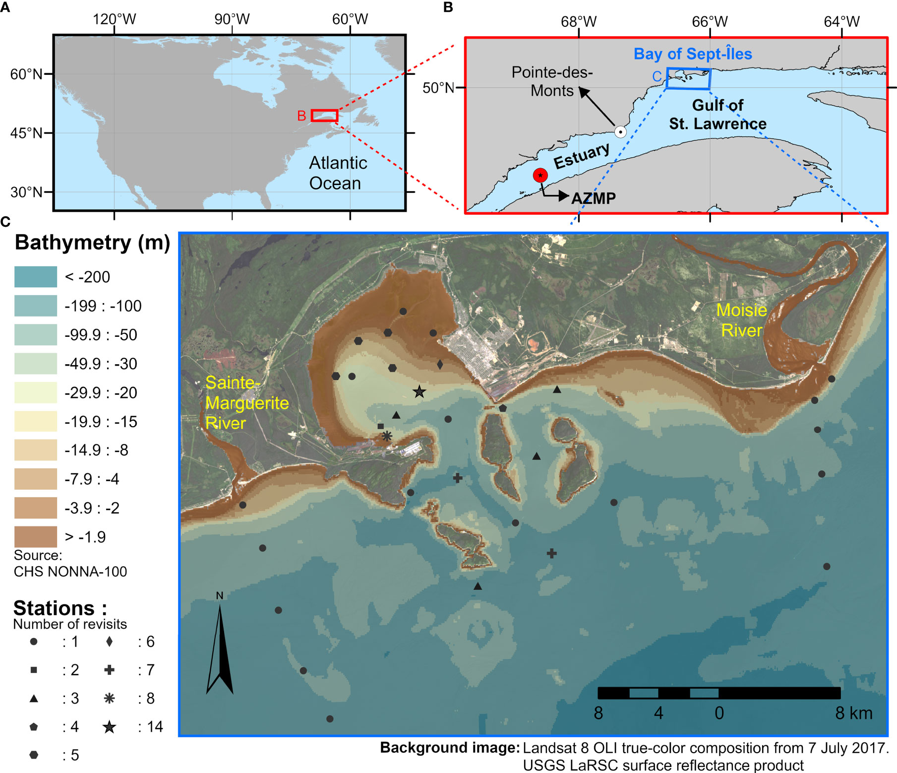
Figure 1 (A) The Estuary and Gulf of St. Lawrence in the North America context, and (B) study area sampling locations: the Bay of Sept-Îles and the AZMP buoy. (C) Spatial distribution and number of revisits of the sampling stations in the Bay of Sept-Îles.

The dataset used in this study consist of in situ profiles and discrete surface water samples collected on an array of stations, within the scope of the interdisciplinary project Canadian Healthy Oceans Network (CHONe2; see Ferrario et al., 2022, for further details about the project). More details about the sampling strategy and methods are found in Araújo and Bélanger (2022). The dataset provided a unique opportunity to investigate the spatial – order of 10⁰ to 10¹ km – and seasonal variability of phytoplankton and bio-optical conditions of the nearshore environment of BSI (Figure 1; Table 1). The stations (Figure 1C) were sampled during seven field campaigns from late spring to early fall 2017 (BSI-1 to BSI-7, from early May to October), and one time in 2019 (BSI-8, early June). For comparison purposes, we also included a station in the middle of the St. Lawrence Estuary (the AZMP – Atlantic Zone Monitoring Program – buoy location, at Rimouski (RIKI) station, Figure 1B), visited on eleven occasions from July to October 2015 (described in Bélanger et al., 2017).

TABLE 1

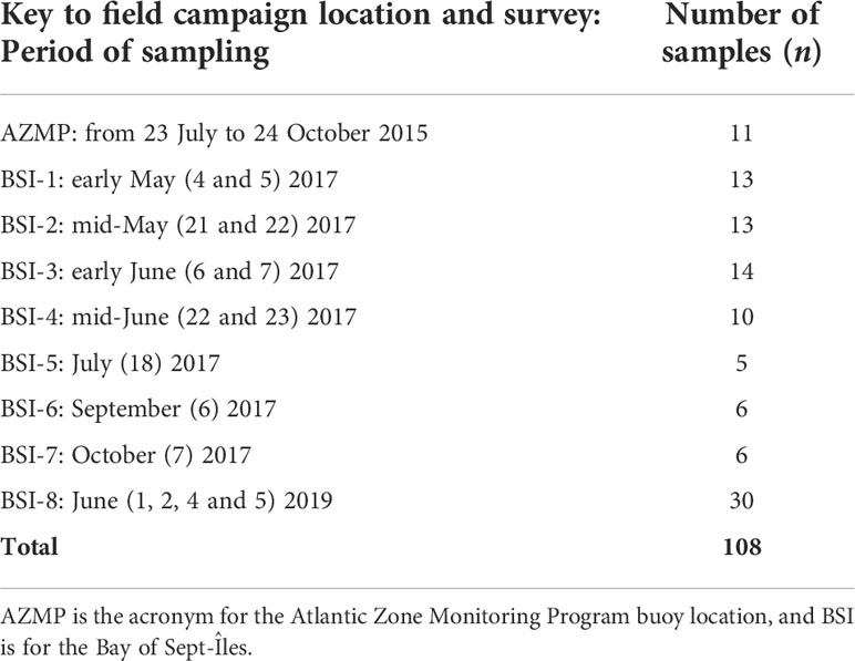
Table 1 Summary of the sampling strategy: Dates and number of water samples.

The discrete surface water samples were collected with a Niskin bottle (or bucket) and were kept cool in dark conditions until further laboratory procedures, which were made each day immediately after the cruise and consisted mainly of filtration operations. Optical and biogeochemical parameters obtained using in situ vertical profiles were matched to the closest measure of the depth of the discrete water sampling. A total of 108 samples was considered in this study (Table 1).

2.2 Phytoplankton assemblages

Phytoplankton assemblages were identified using a combined Principal Component Analysis (PCA) and Hierarchical Cluster Analysis (HCA) procedures, using pigment concentrations and cell abundances grouped in size classes as primary inputs.

Phytoplankton pigments were determined using High Performance Liquid Chromatography (HPLC), following the procedure described by Zapata et al. (2000). Briefly, water samples were filtered through 25 mm (or 47 mm) GF/F glass fiber filters, flash frozen in liquid nitrogen, and stored in cryogenic vials at -80°C until further analysis. The pigment extraction was made using methanol, followed by sonication and centrifugation procedures, before placing the samples in the HPLC analyzer (Agilent Technologies 1200 series). Detection and quantification of the pigments were estimated as described in Bidigare et al. (2005).

A total of twenty accessory pigments were considered in the analysis: chlorophylls b (Chlb), c₁, c₂ and c₃, Mg 2,4 divinyl pheoporphyrin a₅ monomethyl ester (MgDVP), peridinin (Peri), 19’‐butanoyloxyfucoxanthin (But), fucoxanthin (Fuco), neoxanthin, prasinoxanthin, violaxanthin, 19’‐hexanoyloxyfucoxanthin (Hex), diadinoxanthin, alloxanthin (Allo), diatoxanthin, zeaxanthin (Zea), lutein, crocoxanthin, α and β-carotene. Total chlorophyll-a (Chla) was considered as the sum of monovinyl chlorophyll-a, chlorophyllids and the allomeric and epimeric forms of chlorophyll-a.

Autotrophic cells (i.e., phycoerythrin- and phycocyanin-containing cyanobacteria and autotrophic eukaryotes) abundances (in cells mL^-1) were measured by flow cytometry. Duplicate 4 mL samples were placed in cryovials and fixed with glutaraldehyde Grade I (Sigma; 0.1% final concentration) in the dark at room temperature for 15 min, flash-frozen in liquid nitrogen, and then stored at -80°C until analysis. The analysis was made using a CytoFLEX flow cytometer (Beckman Coulter) fitted with a blue (488 nm) and a red laser (638 nm). The forward scatter, side scatter, orange fluorescence from phycoerythrin (582/42 nm BP) and red fluorescence from chlorophyll (690/50 nm BP) were measured using the blue laser. The red laser was used to excite the red fluorescence of phycocyanin (660/20 nm BP). Polystyrene microspheres of 2 µm diameter (Fluoresbrite YG, Polysciences) were added to each sample as an internal standard. Pico- (<2 µm) and nano-autotrophs (2-20 µm) were discriminated based on a forward scatter calibration using algal cultures. Since the abundance of phycocyanin-containing cyanobacteria was generally low (i.e., <100 cells mL^-1), they were not included in the analysis.

Prior to applying the PCA/HCA algorithms, each pigment was normalized by Chla and, together with cell abundances (pico- and nano-autotrophs), were standardized (z-scores), given the different nature (units) of inputs. The normalized and standardized data were then submitted to the PCA and the number of Principal Components (PCs) that explained most of the variability (> 80%) were selected to proceed to the HCA.

The HCA method classifies objects (i.e., phytoplankton pigments and size-class abundances) into groups (or clusters) that are similar. In this study, the clustering approach using Ward’s minimum variance method (Ward, 1963) and paired Euclidean linkage distances was applied (as in Neukermans et al., 2016; and Reynolds and Stramski, 2019). The output of the HCA is a dendrogram in which the user defines a linkage distance cutoff value, which, in turn, will determine the number of clusters. For the optimal linkage distance value retrieval, we used the iterative L method procedure (Salvador and Chan, 2004; Neukermans et al., 2016). We also report the cophenetic correlation (Sokal and Rohlf, 1962), as a measure of how accurately a dendrogram maintains the pairwise distance between data objects.

2.2.1 Size-classes contribution to biomass

The fractional contribution of different size classes of phytoplankton to Chla – f_pico (picophytoplankton, mean diameter [D] < 2 µm); f_nano (nanophytoplankton, D = 2 to 20 µm); and f_micro (microphytoplankton, D > 20 µm) – was examined using two different approaches. The first approach (as in Uitz et al., 2006) uses the weighted contributions of seven diagnostic pigments concentrations (Fuco, Peri, Allo, But, Hex, Zea, and Chlb) to determine $f_{\text{pico}}^{\text{HPLC}}$, $f_{\text{nano}}^{\text{HPLC}}$, and $f_{\text{micro}}^{\text{HPLC}}$. For comparison, a second approach used picophytoplankton cell abundances (cells mL^-1) obtained from flow cytometry analysis. It includes eukaryotes and cyanobacteria cell abundances (A_euk and A_cy, respectively), with Chla cell quotas taken for the prasinophyte Micromonas pusilla (Q_Mic, equal to 2×10^-8 µg Chl cell^-1; Montagnes et al., 1994) and the cyanobacteria Synechococcus sp. (Q_syn, equal to 1×10^-9 µg Chl cell^-1; Morel et al., 1993), respectively. Thus, the fractional contribution of picophytoplankton, $f_{\text{pico}}^{\text{FC}}$, was determined by $f_{\text{pico}}^{\text{FC}}={10}^3\left[\left(A_{\text{euk}}\times Q_{\text{Mic}}\right)+\left(A_{\text{cy}}\times Q_{\text{Syn}}\right)\right]/Chla$.

2.2.2 Taxonomic analysis by light microscopy

Phytoplankton cell identification was performed on selected samples (n = 16) to the lower rank possible (groups, genus, and species). Samples were preserved in acidic Lugol’s solution and kept in the dark at 4°C until analysis. The counting of cells >2 µm was performed using an inverted microscope (Zeiss Axiovert 10) following the Utermöhl method with settling columns of 25 mL (Lund et al., 1958). A minimum of 400 cells were counted over at least three transects of 20 mm. Autotrophic phytoplankton were distributed in 10 taxonomic groups plus a group of unidentified flagellates. Unidentified cells accounted for an average of 20% of total cells abundance and, of those, ~60% were smaller than 5 µm.

2.3 Major nutrients and physical parameters

Concentrations of nitrite (${\text{NO}}_2^{-}$), nitrate (${\text{NO}}_3^{-}$) + ${\text{NO}}_2^{-}$, phosphate (${\text{PO}}_4^{3-}$), and silicate ($\text{Si}{\left(\text{OH}\right)}_4^{4-}$) were determined using a colorimetric method with an Autoanalyzer 3 (Bran + Luebbe), as described in Bluteau et al. (2021). Prior to analytical procedures, water samples were filtered through 25 mm GF/F filters in acid-washed syringes and Swinnex. Concentrations of ${\text{NO}}_3^{-}$ were determined by difference.

High-precision salinity (± 0.0003, in practical salinity units, PSU) was measured on discrete water samples using a calibrated Portasal salinometer (model 8410A, Guildline Instruments, Smiths Falls, ON). In situ vertical profiles of temperature and conductivity were taken using a calibrated CTD probe (SBE19, Sea-Bird Scientific, Bellevue, WA).

2.4 Inherent and apparent optical properties

The spectral backscattering and absorption coefficients (b_b(λ) and a(λ), respectively, in m^-1) are inherent optical properties (IOPs) that are related to the remote-sensing reflectance (R_rs(λ)), an apparent optical property, by the means of R_rs(λ) ∝ b_b(λ)/a(λ) (Morel and Prieur, 1977). Hence, the characterization of the IOPs is a primary requirement for discriminating phytoplankton assemblages when considering optical approaches (Reynolds and Stramski, 2019).

The total absorption coefficient, a(λ), is decomposed by the additive contributions of pure water itself (a_w(λ)), chromophoric dissolved organic matter (a_cdom(λ)), non-algal particles (a_nap(λ)), and phytoplankton (a_phy(λ)) (Eq. 1). Similarly, b_b(λ) is decomposed in backscattering of pure water (b_bw(λ)) and particulate matter b_bp(λ)) (Eq. 2).

$\begin{array}{ll}a\left(\lambda \right)=a_w\left(\lambda \right)+a_{cdom}\left(\lambda \right)+a_{nap}\left(\lambda \right)+a_{phy}\left(\lambda \right)& (1)\end{array}$

$\begin{array}{ll}{b}_b\left(\lambda \right)=b_{bw}\left(\lambda \right)+b_{bp}\left(\lambda \right)& (2)\end{array}$

The determination of the above IOPs for the present dataset is described in Araújo and Bélanger (2022). Briefly, a_cdom(λ), a_nap(λ), and a_phy(λ) were determined using a benchtop PerkinElmer Lambda-850 spectrophotometer, equipped with an integrating sphere (used for particles only). The in situ b_bp was determined at six wavelengths using a HydroScat-6P (HS6) backscattering meter (HOBI Labs Inc., Bellevue, WA), and was corrected for salinity variations and loss due to attenuation along the pathlength. The spectral dependency of b_bp was modelled (non-least-squares algorithm) using a power-law function, as b_bp(λ) = b_bp(λ₀)[λ/λ₀]^γ, where γ is a dimensionless parameter describing the spectral dependency of b_bp relative to a reference wavelength (λ₀; defined as equal to 550 nm in this study). Low residual differences (means < 5%) between measured and modelled values of b_bp assured the validity of this equation on describing its spectral shape in the study area (Araújo and Bélanger, 2022). Seawater absorption and backscattering coefficients were retrieved from tabulated values available in the literature (Morel, 1974; Zhang et al., 2009; IOCCG, 2018).

The R_rs(λ) was derived from in situ radiometric measurements using a Compact Optical Profiling System (C-OPS; Biospherical Instruments Inc., San Diego, CA), and followed the procedures described in Bélanger et al. (2017) and Mabit et al. (2022). Briefly, the system was equipped with sensors that measured the above-water downwelling irradiance, E_d(λ, 0⁺), and the upwelling radiance from vertical profiles in the water column, L_u(λ, z). The processing schema included the extrapolation of L_u(λ, z) to assess the water-leaving radiance, L_w(λ, 0⁺). The R_rs(λ) is then calculated using R_rs(λ) = L_w(λ, 0⁺)/E_d(λ, 0⁺). C-OPS radiometry data are collected at 19 wavelengths, thus, R_rs(λ) was interpolated using a piecewise cubic polynomial function to obtain 1‐nm resolution, while preserving its spectral shape (Reynolds and Stramski, 2019).

2.5 Statistical analysis

Descriptive statistics (mean and standard deviation) and one-way Analysis of Variance (ANOVA) were used to quantitatively compare the populations identified by the clusters obtained by the PCA/HCA procedures. Data were confirmed to exhibit normal distributions using the Lilliefors (or Kolmogorov-Smirnov) test prior to all ANOVAs, and differences between pairs of means (pairwise comparisons) were assessed using the Tukey Honest Significant Difference (Tukey’s HSD) criterion post-hoc test. In the following, when a population of data presents significant difference, it means that ANOVA presented a p-value less than 5% of significance level (p < 0.05). Additionally, when individual groups (clusters) are compared to others (pairwise comparisons), the Tukey’s HSD criterion is used. All data manipulations and statistics were done using MATLAB (MathWorks) software.

3 Results

3.1 Clusters of phytoplankton assemblages

The normalized and standardized phytoplankton pigments concentrations (n = 20) and pico- and nano-autotrophic cell abundances (eukaryotic and cyanobacteria; n = 4) were submitted to the Principal Component Analysis (PCA), and the seven first principal components explained 80.3% of the variance in the data set. In sequence, the projections of the original data on the principal component vector space (scores) were computed and the seven first columns were used as input in the Hierarchical Cluster Analysis (HCA). Figure 2 shows the dendrogram as obtained by HCA, as well as the procedure used to determine the linkage distance and subsequent number of clusters (L method; Salvador and Chan, 2004).

FIGURE 2

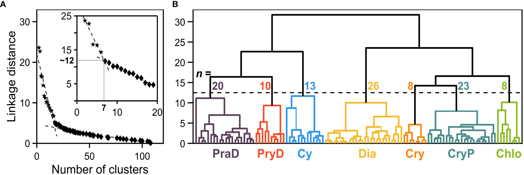
Figure 2 (A) Linkage distance as a function of the number of clusters obtained from the dendrogram (shown in (B)). The L-method (Salvador and Chan, 2004) is first applied considering all dataset (n =108), and then to a restricted range for the number of clusters (inset). The resulting “knee” corresponds to a linkage distance cutoff of 11.9, which divides the input dataset in seven clusters. (B) Dendrogram obtained from the Hierarchical Cluster Analysis. The dashed line corresponds to the linkage distance cutoff, and the number above each cluster shows the corresponding number of samples. The clusters are denoted by PraD (purple), PryD (red), Cy (blue), Dia (yellow), Cry (orange), CryP (teal) and Chlo (green).

The inset of Figure 2A shows the reductional approach necessary to obtain a lower number of groups, consisting of applying the L method to a limited range of possible clusters (Salvador and Chan, 2004; Neukermans et al., 2016). This approach revealed to be more adequate to our analysis, since the obtained linkage distance cutoff (Figure 2B) divided the dataset in seven groups, containing between 8 and 26 samples, in each individual cluster. The cophenetic correlation value for the HCA was 0.62, comparable to other reported values in the literature (e.g., Neukermans et al., 2016).

The variability of selected inputs is shown in Figure 3, whereas the mean and standard deviation of all 24 inputs are presented in Table S1 (Supplementary Material). Only the pigment 19’ butanoyloxyfucoxanthin (But) did not present significant difference considering the seven classes of phytoplankton assemblages (one-way ANOVA, p > 0.05). The analysis of cell abundances and pigments to Chla ratios within the groups revealed a complex co-occurrence of diverse phytoplankton groups, as the assignment of taxonomic classes from pigment signatures is not always a straight-forward task (Roy et al., 1996). Despite these inherent limitations, we assessed characteristics of each group that could be used to distinguish them from the others. For such analysis, we used available information compiled in the literature that links phytoplankton pigments to taxonomic classes (e.g., Roy et al., 1996; Gibb et al., 2000; Kramer and Siegel, 2019).

FIGURE 3

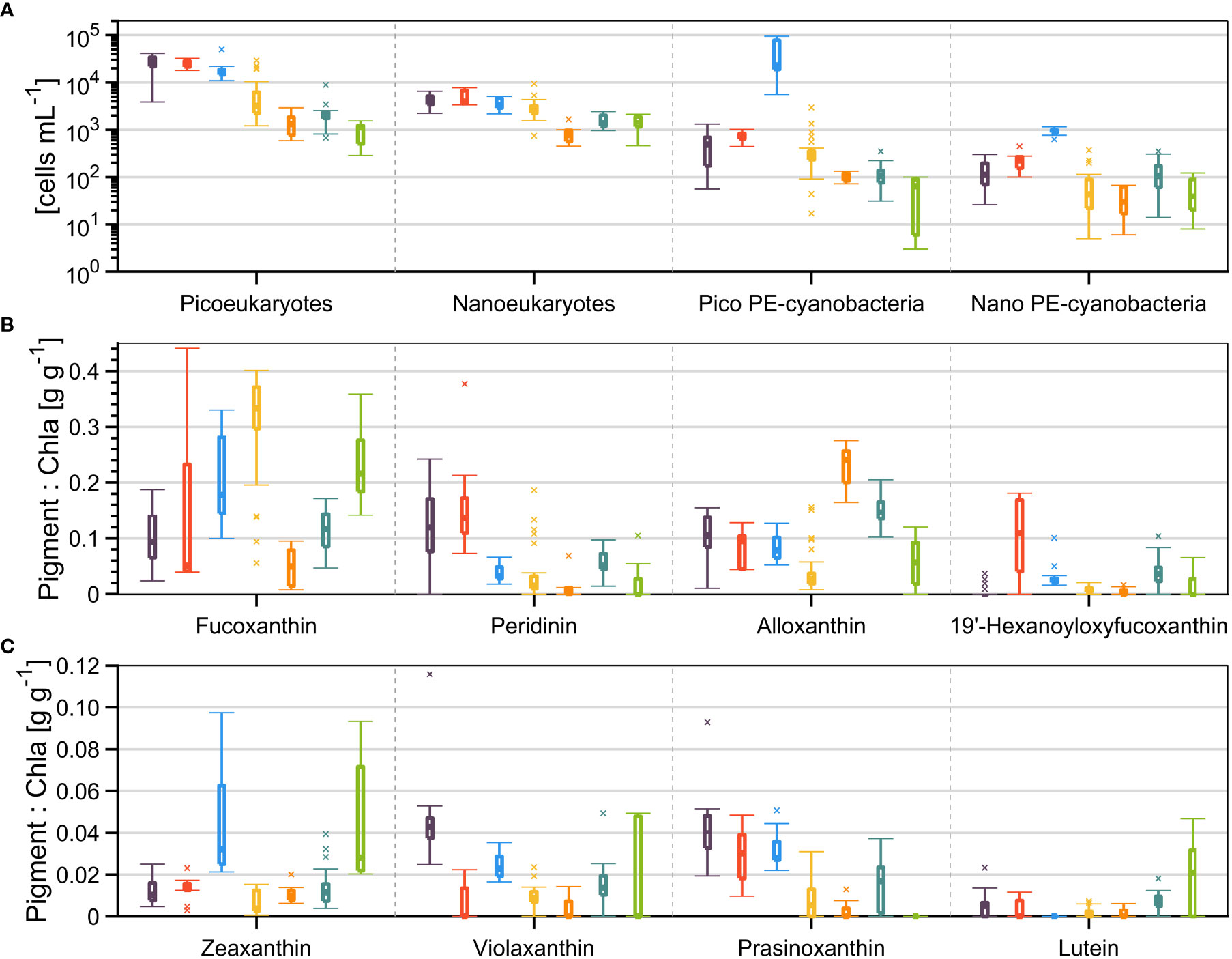
Figure 3 Variability (median, 25th and 75th percentiles, minimum, maximum and outliers) of (A) four classes of phytoplankton cell abundances (B, C) and eight accessory pigments to Chla ratios concentrations. The autotrophic cells concentration is separated by eukaryotes and phycoerythrin-containing (PE-) cyanobacteria, and by pico- (<2 μm) and nano-size (>2 and <20 μm) classes. The color code, associated to each cluster group, is the same as in Figure 2.

The relative distribution of phytoplankton groups identified by light microscopy (LM) are presented in Figure S1 (Supplementary Material). The correspondence between the seven clusters and the taxonomic analysis by LM was not straight-forward. First, LM resolution limits the identification of cells smaller than 3 µm. Second, the strong coloration of the acidic Lugol’s solution used the preserve the samples make it difficult to distinguish autotrophic from heterotrophic cells using LM (see Tremblay et al., 2009). On the contrary, HPLC pigment concentrations and flow cytometry measurements both account for autotrophic cells smaller than 3 µm. Moreover, a high number of unidentified cells (average 20%) and, specifically, unidentified flagellates (between 25 and 50%, Figure S1) were assigned by the LM technique. Nevertheless, LM analysis revealed the presence of important species that helped in the interpretation of the composition of the phytoplankton assemblages.

The first cluster (purple) presented the highest means (and significantly higher than almost all other groups) picoeukaryotes cell counts and Chla-normalized pigment concentrations of neoxanthin, prasinoxanthin, violaxanthin, and Chl b. Moreover, there were significantly higher means (although not the highest) concentrations of nanoeukaryotes, Chl c₁, β-carotene and Perid. From these characteristics, we related this group to the presence of prasinophytes (possibly Micromonas sp.) and dinoflagellates (hereafter referred to as PraD). From the LM analysis, the prasinophyte Pyramimonas sp. was representative for the group PraD.

The second cluster (red) presented the highest means of nanoeukaryotes, Perid, Hex, and diadinoxanthin, while picoeukaryotes, Chl c₁ and c₂, prasinoxanthin and β-carotene were also significantly higher than other groups (but not the highest). We related this group to a relative dominance of prymnesiophytes and dinoflagellates (PryD). The LM analysis confirmed the presence and a relatively high abundance of the prymnesiophyte Chrysocromulina spp. in this group. The dinoflagellates Gymnodinum spp. and Heterocapsa rotundata were always representative in samples of groups PraD and PryD, while the toxic A. tamarense was also identified in these groups. Interestingly, the maximum concentration of A. tamarense (2920 cells L^-1) was observed in an anomalous sample (PryD-B, Figure S1) with a very high concentration of the diatom Skeletonema costatum.

The third cluster (blue) presented the highest means of pico- and nano-phycoerythrin-containing cyanobacteria, Zea, Chl c₃, and β-carotene, but also higher picoeukaryotes, neoxanthin, prasinoxanthin and Chl b. Thus, this group was related to a marked characteristic of occurrence of cyanobacteria (Cy), possibly Synechococcus sp. While presenting relatively high Fucoxanthin to Chla, the LM revealed in this group high abundances of the diatoms Lennoxia faveolata, Leptocylindrus minimus, Skeletonema costatum, Thalassiosira conferta, and Chaetoceros spp., but also the dinoflagellate H. rotundata.

The fourth (yellow) and most numerous cluster (n = 26) presented the highest means of Fuco, Chl c₁ and c₂, and was attributed to a dominance of diatoms (Dia). Cells enumerated by LM analysis revealed high abundances of the genus Chaetoceros (C. debilis, C. convolutes, C. gelidus, and Chaetoceros spp.) and the species Thalassiosira nordenskioeldii. Furthermore, the taxonomic groups identification of samples from group Dia revealed higher dominance of diatoms in relation to others (>50%, Figure S1), as expected.

The fifth (orange) and sixth (teal) clusters both presented the highest means of Allo and crocoxanthin, but the former had the highest means of α-carotene, while the latter had the highest means of MgDVP. We attributed these groups to be related to a marked presence of cryptophytes, but the sixth group had some important contribution from prasinophytes. Therefore, these groups were denoted as Cry and CryP, respectively, with Hemiselmis virescens and Plagioselmis prolonga var. nordica being representative species. Moreover, these two groups were the most similar based on the dendrogram (Figure 2B). Finally, the seventh (green) cluster presented the highest mean of lutein, but also significantly higher concentrations of Zea than other groups (except Cy). We attributed this group to a relatively greater contribution of chlorophytes (Chlo) to the phytoplankton assemblages.

The numerical abundance of micro-, nano-, and pico-phytoplankton size-classes were examined in Figure S2. First, nanophytoplankton abundances obtained from flow cytometric measurements were compared to those obtained by light microscopy (LM), including unidentified cells (Figure S2A). Both measurements are comparable in terms of absolute values, but LM systematically underestimates the number of cells, comparatively, indicating a limitation of the former method to adequately account for this size class. Furthermore, a comparison of distribution of the three size-classes abundances (Figure S2B, with microphytoplankton abundances retrieved from the LM analysis) revealed a strong numerical dominance of picophytoplankton in all samples, except five samples where picophytoplankton represented ~50% of total cell abundance.

The fractional contribution of phytoplankton size classes to Chla (f_pico, f_nano, and f_micro) are shown in Figure 4. The two methods used to estimate f_pico ($f_{\text{pico}}^{\text{FC}}$ and $f_{\text{pico}}^{\text{HPLC}}$) were compared (Figure 4A) and presented a coefficient of determination (R²) of 0.35. In general, the correspondences between the two methods presented different patterns when considering the different groups, with $f_{\text{pico}}^{\text{FC}}$ underestimating f_pico in comparison to $f_{\text{pico}}^{\text{HPLC}}$, especially for the groups Dia, Cry, CryP, and Chlo, which were restricted to the lower range of variability (<25%). Nevertheless, the groups with higher values of f_pico, PraD and Cy, were noticeable in both methods.

FIGURE 4

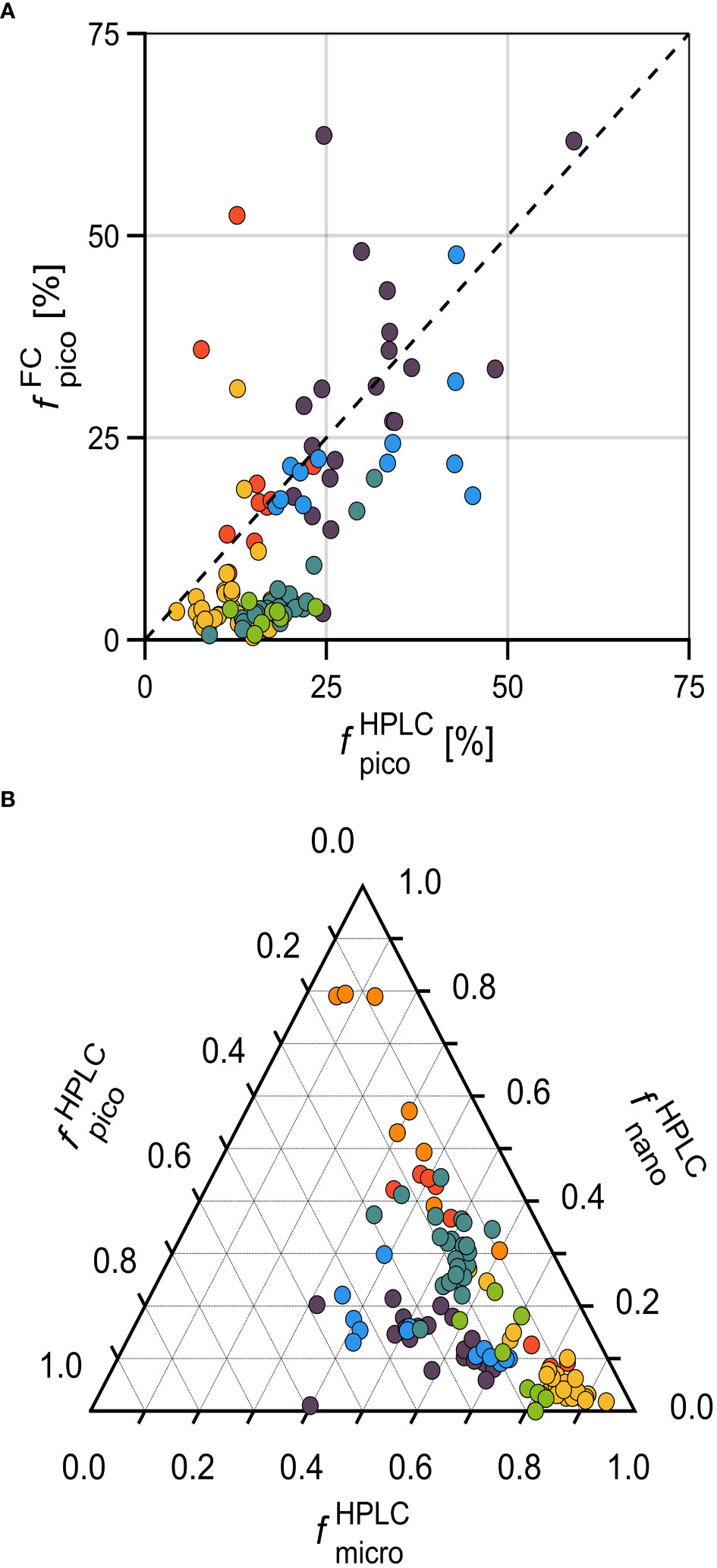
Figure 4 Relative (or fractional, f) contributions of phytoplankton size classes to Chla, for each phytoplankton cluster. (A) Two methods to obtain the picophytoplankton fractional contribution to Chla (f_pico): $f_{\text{pico}}^{\text{FC}}$ and $f_{\text{pico}}^{\text{HPLC}}$ (see text for details). (B) Ternary plot of $f_{\text{pico}}^{\text{HPLC}}$, $f_{\text{nano}}^{\text{HPLC}}$, and $f_{\text{micro}}^{\text{HPLC}}$. This approach (pigment-based) considers a global relationship using seven diagnostic pigments as inputs (Uitz et al., 2006). The color code is the same as in Figure 2.

Although the Uitz et al. (2006) method (used to determine f^HPLC) was developed using global relationships and may have constraints on applying to a coastal/nearshore dataset, as the one presented in this study, we investigated the size fractioned contributions of phytoplankton in the ternary diagram presented in Figure 4B. The different clustering groups presented distinguishable patterns of distribution. Most samples presented $f_{\text{micro}}^{\text{HPLC}}$ higher than 50%, with the most noticeable contribution of this fraction for Dia. Specifically, the groups PraD and Cy presented a dispersion from $f_{\text{micro}}^{\text{HPLC}}$ towards $f_{\text{pico}}^{\text{HPLC}}$, while this dispersion for the groups CryP, PryD, and, particularly for Cry, were towards $f_{\text{nano}}^{\text{HPLC}}$.Overall, the phytoplankton communities were well discriminated by the PCA/HCA procedures. Despite the picophytoplankton numerical dominance, the total biomass was dominated by microphytoplankton, with some variations within clusters.

3.2 Seasonal and spatial variability

The Chla biomass, the seasonal succession, and spatial variabilities within phytoplankton clusters are shown in Figure 5. In Bay of Sept-Îles (BSI), Chla medians were always between 1 and 3 mg m^-3 for all groups, except for Chlo whose median is 0.66 mg m^-3 (Figure 5A). No group is significantly different from the others, but PryD and Dia presented higher means of Chla. In comparison, only two groups were present at AZMP (Dia and PraD) in the middle of the Lower St. Lawrence Estuary, during the period from July to October 2015, and Chla values were generally higher than in BSI, with values ranging from 1.02 to 11.43 mg m^-3 (Figure 5B).

FIGURE 5

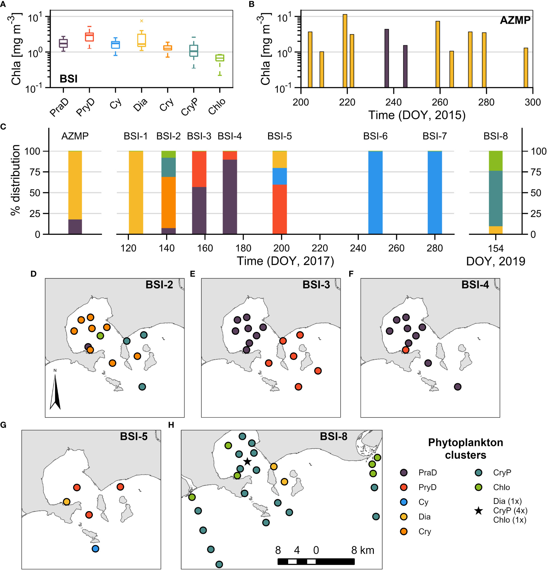
Figure 5 Temporal and spatial variability of the phytoplankton clusters. (A) Boxplots showing the variability of Chla for each cluster, for the Bay of Sept-Îles (BSI). (B) Bars showing the temporal variability of Chla in the AZMP buoy station (DOY = Day of Year). The color of the bars corresponds to the class of phytoplankton clusters. (C) Relative distribution of phytoplankton clusters for AZMP and for the temporal series in BSI (BSI-1 to 8; Table 1). (D–H) Spatial distribution for each campaign that presented noticeable variability of phytoplankton clusters.

The seasonal evolution of the phytoplankton clusters of BSI are shown in Figure 5C, where the bars represent the relative contribution of each group during each campaign. Firstly, in early May 2017 (BSI-1) only the group Dia was found in BSI surface waters. About two weeks later (BSI-2), the group Dia was replaced mainly by the groups Cry, CryP, and Chlo. Interestingly, the dominance of groups CryP and Chlo (but also some samples from Dia) was also observed in the field campaign of early June 2019 (BSI-8). In June 2017 (BSI-3 and 4) only groups PraD and PryD were found in BSI, followed in July (BSI-5) by the occurrence of PryD, Dia, and Cy. Finally, only group Cy was found in fall (BSI-6 and 7).

Although BSI-1, 6, and 7 were characterized by a single group, the other field campaigns presented heterogeneity regarding the phytoplankton assemblages, and their spatial distribution is shown in Figures 5D–H. The dominant groups in BSI-2, Cry and CryP, were generally found inside and outside the bay, respectively (Figure 5D). This spatial separation was even clearer in BSI-3 for the groups PraD (inside) and PryD (outside the bay). In BSI-5, the sample correspondent to Cy is in a station outside the bay. In the 2019 campaign (BSI-8), beside the dominance of CryP, the group Chlo was distributed in the riverine (freshwater) plumes, while two Dia samples were distributed in-between the islands east of the bay. These results evidence the seasonal succession of phytoplankton assemblages, but reveal that the spatial variability, at this scale, is also important.

3.3 Major nutrients and physical environment

The relationships between major nutrient concentrations, associated to each phytoplankton assemblage, are shown in Figures 6A, B, and the physical environment, as determined by temperature and salinity, are shown in Figure 6C. The mean and standard deviation of each variable for the Bay of Sept-Îles (BSI) of Figure 6 (plus nitrite and nutrient concentrations ratios) are summarized in Table 2. Samples from the Lower St. Lawrence Estuary (AZMP, squares in Figure 6) were differentiated from those of BSI. In addition, other samples from BSI were considered as outliers. First, two samples from the group Dia, in the campaign BSI-8 (Figure 5H), had environmental (and optical) characteristics typical of those from the group Chlo. This might be related to lateral advection of phytoplankton cells. Secondly, few samples from groups Chlo (2) and CryP (1) were found to have anomalous values of physical and optical (not shown) variables. These samples were obtained in turbulent hydrodynamic conditions close to riverine discharges. Water sampling might not reflect the same conditions as the data acquired by the in situ instrumentation (CTD, HS6, C-OPS). In the following, these outliers are not considered.

FIGURE 6

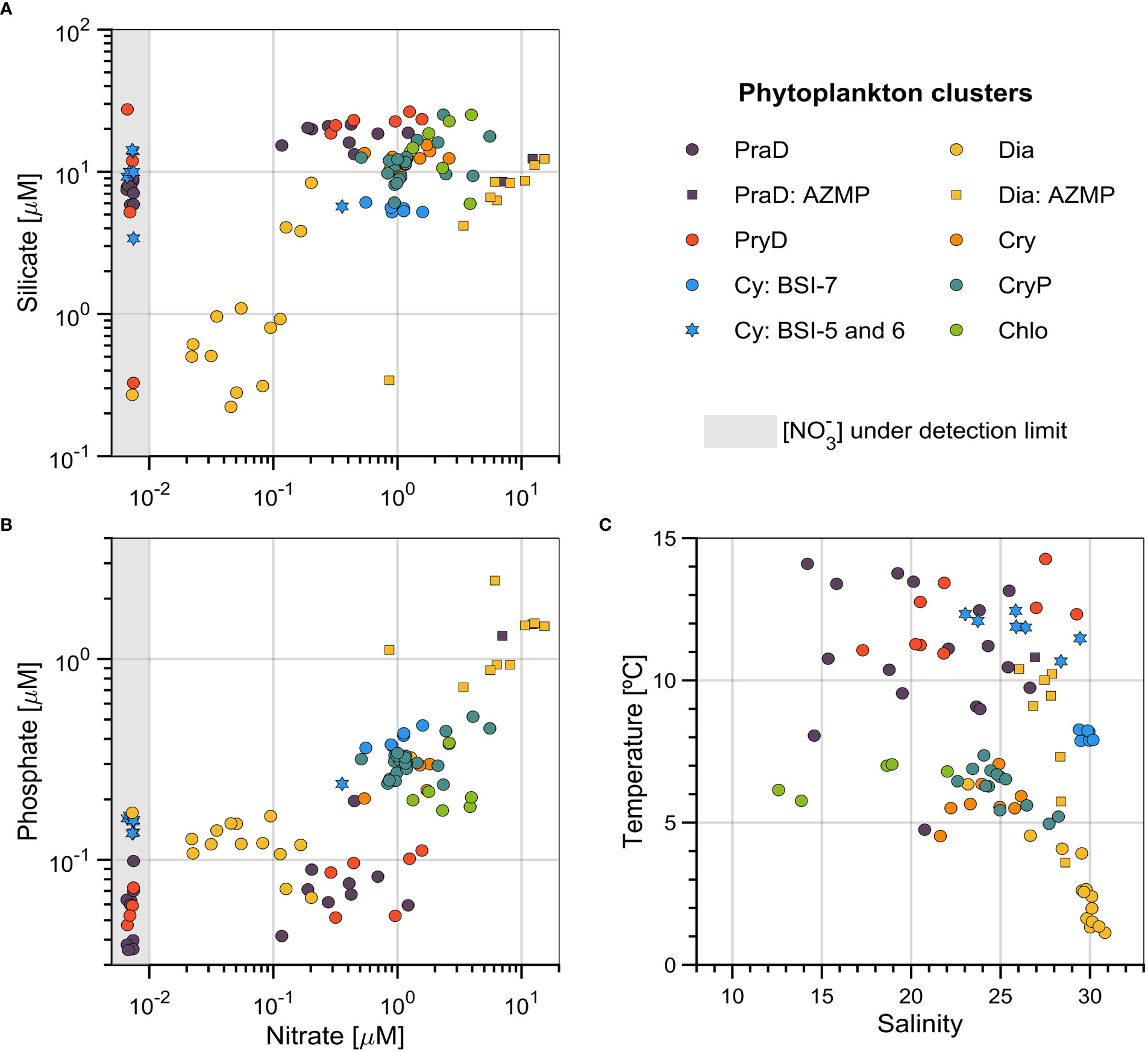
Figure 6 Nutrient concentrations and physical parameters relationships associated with each phytoplankton cluster. (A) Silicate ([$\text{Si}{\left(\text{OH}\right)}_4^{4-}$) versus nitrate ([${\text{NO}}_3^{-}$); (B) phosphate ([${\text{PO}}_4^{3-}$) versus nitrate concentrations; and (C) temperature versus salinity. Samples from the Lower St. Lawrence Estuary station (AZMP) are presented by squares, and outliers from the Bay of Sept-Îles (BSI) are presented by diamonds. The gray-shaded area corresponds to undetectable nitrate levels (~0 µM).

TABLE 2

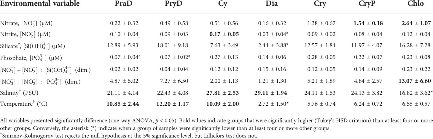
Table 2 Mean and (plus or minus) standard deviation of nutrient concentrations and physical parameters for each of the seven clusters of phytoplankton (PraD, PryD, Cy, Dia, Cry, CryP, and Chlo), for the Bay of Sept-Îles (BSI) region.

The nutrients and physical environment at the Lower St. Lawrence Estuary station (AZMP) are markedly different from those of BSI, when considering the same phytoplankton groups of these two locations. Nitrate and phosphate concentrations values were higher for AZMP (Figure 6B), while silicate concentrations were similar (Figure 6A). However, if only the group Dia is considered, silicate concentrations were also higher at AZMP (except for one sample). Interestingly, the Dia samples from AZMP were also associated with higher temperatures (mean of 8.2°C) than the ones from BSI (mean of 2.7°C), but with slightly lower salinities (means of 27.6 and 29.1, for AZMP and BSI, respectively) (Figure 6C).

All nutrient concentrations, nutrient ratios, and physical parameters were significantly different for the seven phytoplankton clusters (one-way ANOVA, p < 0.05). Samples from BSI-4, BSI-5, and BSI-6 (stars in Figure 6) field campaigns (Figure 5C, from mid-June to early September 2017) presented undetectable nitrate concentration (~0 µM). Thus, depleted nitrate conditions were noticeable for samples of groups PraD, PryD and Cy (right side of Figures 6A, B). Although we do not differentiate these samples from others of the same group in Table 2, silicate concentrations values for these population of samples were generally lower for PraD and PryD (comparing to the same groups in BSI-3), and higher for Cy (comparing to the same group in BSI-7). Notwithstanding, phosphate concentrations values (in the nitrate-depleted conditions) were comparable with others for PraD and PryD, and slightly lower for Cy. A single sample from group Cy (BSI-6) presented a nitrate concentration much higher than the detection limit (~0.36 µM), and it corresponded to the station farthest from the shore.

The nitrate concentrations associated to the different groups in BSI, as analyzed by pairwise comparisons (Tukey’s HSD criterion), revealed that Chlo has higher concentration than all other groups, while CryP was higher than PraD, PryD, Cy, and Dia. Nitrite concentrations was higher in Cy than all other groups (except Chlo), while Dia has significantly lower concentrations than all other groups.

In non-depleted [${\text{NO}}_3^{-}$] conditions, silicate concentrations (Figure 6A; Table 2) in groups PraD, PryD, and Cy presented very low variability. In Dia, silicate concentrations were significantly lower than all other groups (except Cy). Two groups, PraD and PryD, presented significantly lower values of phosphate concentrations (Figure 6B; Table 2) than others (Cy, Cry, CryP, and Chlo). Moreover, [${\text{PO}}_4^{3-}$] in Chlo was significantly higher than Dia (besides Prad and PryD).

Nutrient ratios are commonly used to assess elemental limitation for phytoplankton production. The nitrate (plus nitrite) to silicate and the nitrate (plus nitrite) to phosphate ratios (dimensionless) are presented in Table 2. The $\left[{\text{NO}}_3^{-}\right]+\left[{\text{NO}}_2^{-}] : [\text{Si}{\left(\text{OH}\right)}_4^{4-}\right]$ means were lower for groups PraD and PryD and highest for group Chlo. Nevertheless, Chlo also presented higher $\left[{\text{NO}}_3^{-}\right]+\left[{\text{NO}}_2^{-}] : [{\text{PO}}_4^{3-}\right]$ means than all other groups (minus PryD), while Dia was significantly lower than Chlo and PryD.

The groups PraD, PryD, and Cy were found in warmer waters than the other groups (Figure 6C; Table 2). Conversely, the group Dia presented significantly lower temperatures when compared to all other groups. Dia and Cy (specifically the blue circles in Figure 6) were found in saltier waters (>28), while group Chlo presented significantly lower salinities than all other groups but PraD. Also noticeable is the narrow range of temperature (~8 °C) and salinity (~30) of some samples of group Cy, which were collected on BSI-7 (October 2017, Figure 5C). The groups associated with the presence of cryptophytes, Cry and CryP, and Chlo, presented low variability of temperatures (small standard deviation, Table 2).

The separation of group Cy between campaigns BSI-5 and 6 (stars in Figure 6) and BSI-7 were done because of the different environmental conditions in which the two sets of samples were found (e.g., nitrate depletion, temperature, salinity). The set of samples of group Cy in BSI-5 and 6 presented more similar environmental conditions to those of groups PraD and PryD. Optical conditions of group Cy from BSI-5 and 6 were also closely related to these groups (not shown). Therefore, in the following presentation of results only the set of BSI-7 are considered for the group Cy.

3.4 Optical characterization

The total and component-specific spectral absorption and backscattering coefficients are presented in Figure 7. For each graph (A-F), each phytoplankton group curve is represented by the sample having the highest counts of median values, calculated for unitary wavelength within the visible spectral range (400 to 700 nm). Descriptive statistics and tests for some optical properties shown in Figures 7, 8 are presented in Table 3, for selected wavelengths, in the perspective of satellite remote sensing applications.

FIGURE 7

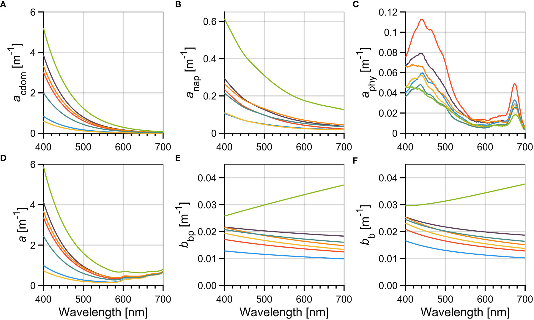
Figure 7 Inherent optical properties spectra: absorption coefficients of (A) chromophoric dissolved organic matter (a_cdom); (B) non-algal particles (a_nap); and (C) phytoplankton (a_phy); (D) total absorption coefficient (a); (E) particulate backscattering (b_bp); and (F) total backscattering coefficient (b_b). For each graph, the different lines represent the median spectra for each cluster of phytoplankton groups, and the color code is the same as in Figure 2.

FIGURE 8

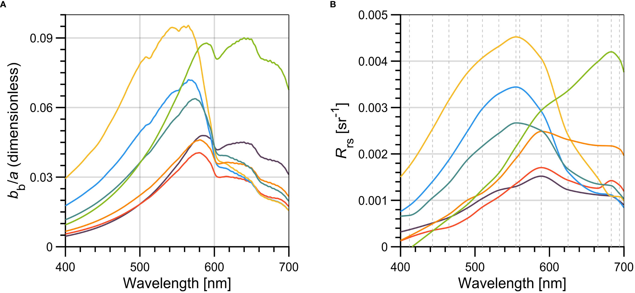
Figure 8 Spectra of (A) the ratio of total backscattering to total absorption coefficients (b_b/a), and (B) the measured remote sensing reflectance (R_rs). The vertical gray dashed lines on (B) indicates the original spectral bands of the C-OPS instrument used to derive R_rs. For each graph, the different lines represent the median spectra for each cluster of phytoplankton groups, and the color code is the same as in Figure 2.

TABLE 3

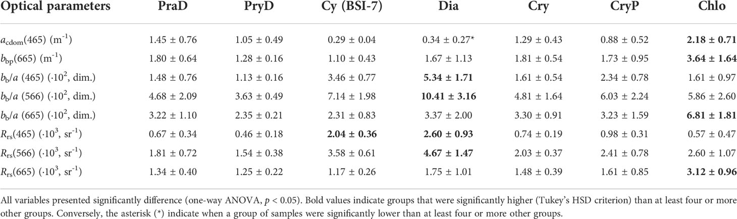
Table 3 Mean and (plus or minus) standard deviation of temperature, inherent optical properties (including ratios), and remote sensing reflectance, at selected wavelengths, for each of the seven clusters of phytoplankton (PraD, PryD, Cy, Dia, Cry, CryP, and Chlo).

For most phytoplankton assemblages, CDOM absorption coefficient (a_cdom, Figure 7A) was approximately one order of magnitude higher than the other absorption components at wavelengths shorter than 500 nm. As expected, the group Chlo, found in fresher waters (Table 2) presented significantly higher a_cdom(465) than other groups, minus PraD and CryP (Table 3). In contrast, groups more related to marine end-member waters (with saltier characteristics), such as Dia and Cy, presented lower values of a_cdom(λ).

The non-algal particles absorption spectra (a_nap, Figure 7B) were much lower than a_cdom, but had similar relative magnitudes when considering individual groups of phytoplankton, suggesting a co-variation between these two optical components. For example, a_nap(465) in group Chlo was significantly higher than all others, while Dia and Cy values were significantly lower than for PraD and Cry.

The phytoplankton absorption coefficient spectra (a_phy, Figure 7C) was also much lower than a_cdom or a_nap and, thus, its influence in the total absorption coefficient (a , Figure 7D) is minimal (see also Araújo and Bélanger, 2022). For example, the fractional contribution of a_phy to the non-water absorption coefficient (= a_cdom + a_nap + a_phy) was maximal in the blue peak of a_phy(~465 nm), but higher mean values reached only 6.2 and 5.4% for groups Dia and Cy. Nevertheless, significantly higher values of a_phy(465) and a_phy(665) were found for group PryD, which also presented higher Chla values (Figure 5A).

As expected, the a(λ) reflects the additive effects of a_cdom and a_nap, especially in the blue and green regions of the spectrum, while in the red the pure water absorption (a_w) dominates the absorption budget.

The particulate (b_bp) and total (b_b) backscattering coefficients are shown in Figures 7E, F. Most phytoplankton groups presented similar spectral characteristics of b_bp (and b_b), but group Chlo was higher than others at all wavelength ranges. Interestingly, the spectral variability of b_bp from group Chlo presented an odd behavior compared to the others, with increasing values with increasing wavelength. This group has significantly higher values of the spectral slope (γ) of b_bp, resulting in significantly higher b_bp(655) (Table 3).

The spectra of backscattering to total absorption coefficient ratio (b_b/a) and the remote sensing reflectance (R_rs) are shown in Figure 8, for each phytoplankton assemblage. As for individual IOPs (Figure 7) the b_b/a and R_rs shown for each group corresponds to the mode (spectral domain) of median values for individual wavelengths. Although similarities are expected when comparing these two variables, it is important to note that inelastic scattering by water molecules (Raman) and by CDOM and phytoplankton pigments (fluorescence) are not considered in b_b/a. Furthermore, the approach we used does not consider changes in IOPs along the water column, that could result in changes in the light field in highly stratified waters (particularly in L_w, and consequently in R_rs). Notwithstanding, this latter situation is likely to happen under some circumstances in our study area (Araújo and Bélanger, 2022).

Most phytoplankton groups presented similar shape and magnitudes of the b_b/a spectra, observed in all wavelength ranges. The two exceptions were for groups Dia and Chlo that peaked in green (~560 nm) and red (~640 nm) regions, respectively. The combination of lower a and at-average b_b values give significant higher values of b_b/a in the blue (465) and green (566) regions for group Dia (Table 3). Similarly, the significantly higher values of b_b/a (665) for the group Chlo is explained by the high b_bp in the red region associated with this group, which is found in waters heavily influenced by terrigenous inputs.

Dissimilarities between b_b/a and R_rs were observable mainly in the red spectral range (>620 nm) and are mostly due to inelastic scattering processes affecting R_rs. However, the characteristics of b_b/a spectra that are distinguishable for the phytoplankton groups Dia and Chlo are also observed in R_rs (Figure 8B; Table 3).

3.5 Seasonal succession and framework for remote sensing estimations

The variability of phytoplankton assemblages and nutrient concentrations, physical parameters, and optical properties revealed a clear seasonal signal, as summarized in Figure 9. Since riverine discharges are a major controlling factor in the optical environment in the BSI region (Araújo and Bélanger, 2022), the Moisie River discharge for years 2017, 2019, and the climatological median (1965-2021) is depicted in Figure 9A. It is expected to reflect the seasonality of the smaller rivers discharging directly into the bay (i.e., rivières Hall, des Rapides, aux-foins, du Poste). The values of the discharge peaks of 2017 and 2019 (~2,500 m³ s^-1) were 60% higher than the historical median (from 1965 to 2021).

FIGURE 9

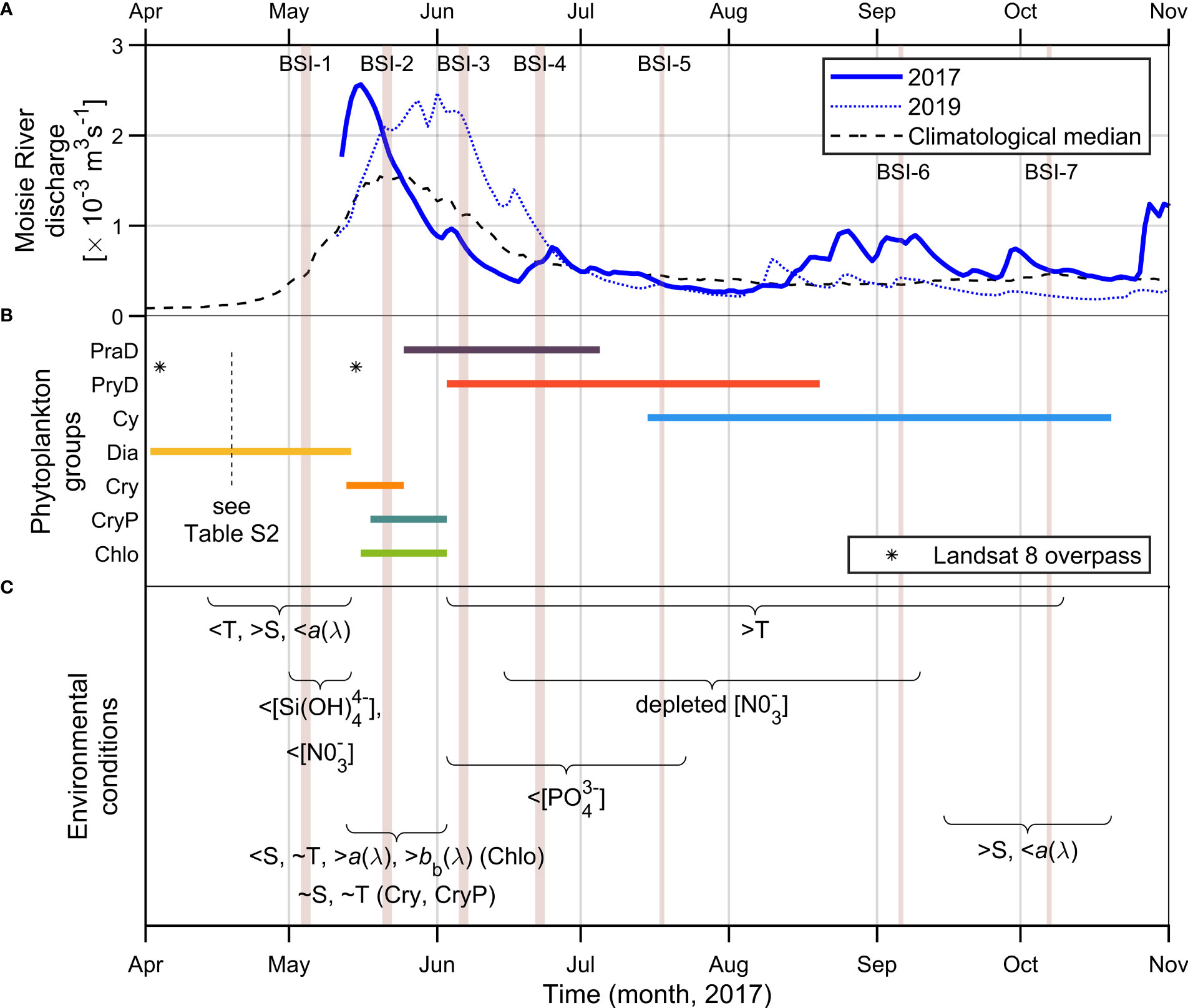
Figure 9 Seasonal succession of phytoplankton assemblages in the Bay of Sept-Îles (BSI). (A) Moisie River discharge for years 2017, 2019, and climatological median (1965-2021). Source: Ministère de l'Environnement et de la Lutte contre les changements climatiques (https://www.cehq.gouv.qc.ca/). (B) Phytoplankton assemblages distribution (see Table S2 in Supplementary Material for details of samples collected in April 19) and dates of Landsat 8 overpass in BSI (shown in Figure 11); and (C) environmental conditions as showed by nutrient concentrations and physical parameters (Temperature and Salinity, T and S) along the year 2017. The durations of the events of both occurrence of phytoplankton assemblages and environmental conditions are extrapolated from punctual field campaigns (BSI-1 to BSI-7, refer to Table 1), represented by vertical light gray lines.

The group Dia occurred in BSI in April - early May (Figure 9B), before the spring freshet, and is related to the spring bloom, a common feature at high latitude estuaries (Carstensen et al., 2015). Lower water temperatures and the lowest light absorption characteristics (due to lower a_cdom and a_nap) are found.

Our interpretation of the spring bloom starting in the BSI region earlier than BSI-1 campaign (early May) is supported by samples collected in mid-April 2017 (Table S2, not used in this study due to incomplete dataset), where biomass (Chla) and Fucoxantin to Chla ratio were among the highest. The Dia samples observed in campaign BSI-1 were likely related to the end of the spring bloom, as indicated by the low nitrate and silicate concentrations. The presence of a subsurface chlorophyll maximum (SCM), a common feature in the Gulf of St. Lawrence (Vandevelde et al., 1987), was observed during field campaign BSI-1 (see Figure S3; Supplementary Material), with similar phytoplankton composition despite much higher Chla values (Table S2). Silicate and phosphate concentrations were comparable at the surface and within SCM, although SCM nitrate levels were one order of magnitude higher than surface samples.

The groups associated with cryptophytes, Cry and CryP, occurred approximately in phase with the peaks of the spring freshet (Figure 9B), and were characterized by an increase in temperature and decreasing salinities. As expected, the freshet increased the amount of CDOM and non-algal particles in the water column, increasing its absorbing and backscattering characteristics. Samples collected in the 2019 field campaign (BSI-8), in early June, had similar characteristics to those collected in BSI-2 (mid-May 2017), reflecting the timing of freshet peaks in each year.

The group Chlo was also dominant during the spring freshet and was found in the vicinity of river plumes (Figure 5H), characterized by lower salinities. This group was characterized by lower Chla values than others and was associated with very turbulent conditions (field observation). The significantly higher nitrate to phosphate ratio in this group (Table 2) reflects the generally higher values of [${\text{NO}}_3^{-}$] in the riverine endmembers (data not shown), in comparison to marine samples. Moreover, the suspended sediment- and CDOM-laden waters of river plumes waters generate the highest absorption and backscattering coefficient values of BSI. The highest b_b (and b_bp) values in the red portion of the spectrum characteristic of Chlo are explained by higher values of the spectral slope of b_bp (γ), which likely reflects higher concentrations of particulate organic matter (Araújo and Bélanger, 2022).

After the spring freshet, as water temperature continue to increase, the groups PraD and PryD occupied the BSI region, and this lasted throughout the summer. Significant lower phosphate concentrations were found to be associated with these two groups (Table 2), while nitrate depletion occurred a few days after their appearance (in-between BSI-3 and BSI-4 campaigns, Figure 9B). The nitrate-depleted conditions then continued in summer up to early fall.

The group dominated by PE-containing cyanobacteria, Cy, began dominating BSI waters in early fall, although its presence was already noted in mid-summer at the station farthest from the shore (BSI-5, Figure 5G). In mid-fall (BSI-7) nitrate concentrations were restored (Figure 6A and Table 2).

The shape and relative magnitudes of remote sensing reflectance (R_rs(λ)) reflected the importance of the bio-optical environment for the determination of phytoplankton assemblages in nearshore waters of BSI. Strong differences in R_rs (Figure 8B; Table 3), in the blue, green, and red bands (465, 566, and 665 nm, respectively), and in SST (Figure 6C; Table 2) between assemblages of phytoplankton suggested the potential of using multispectral and thermal infrared radiometer sensors onboard Earth Observation platforms to infer about them. An inverse framework where SST, R_rs(645), R_rs(566), and R_rs(665) are used as inputs in the classification of BSI waters is therefore proposed (Figure 10).

FIGURE 10

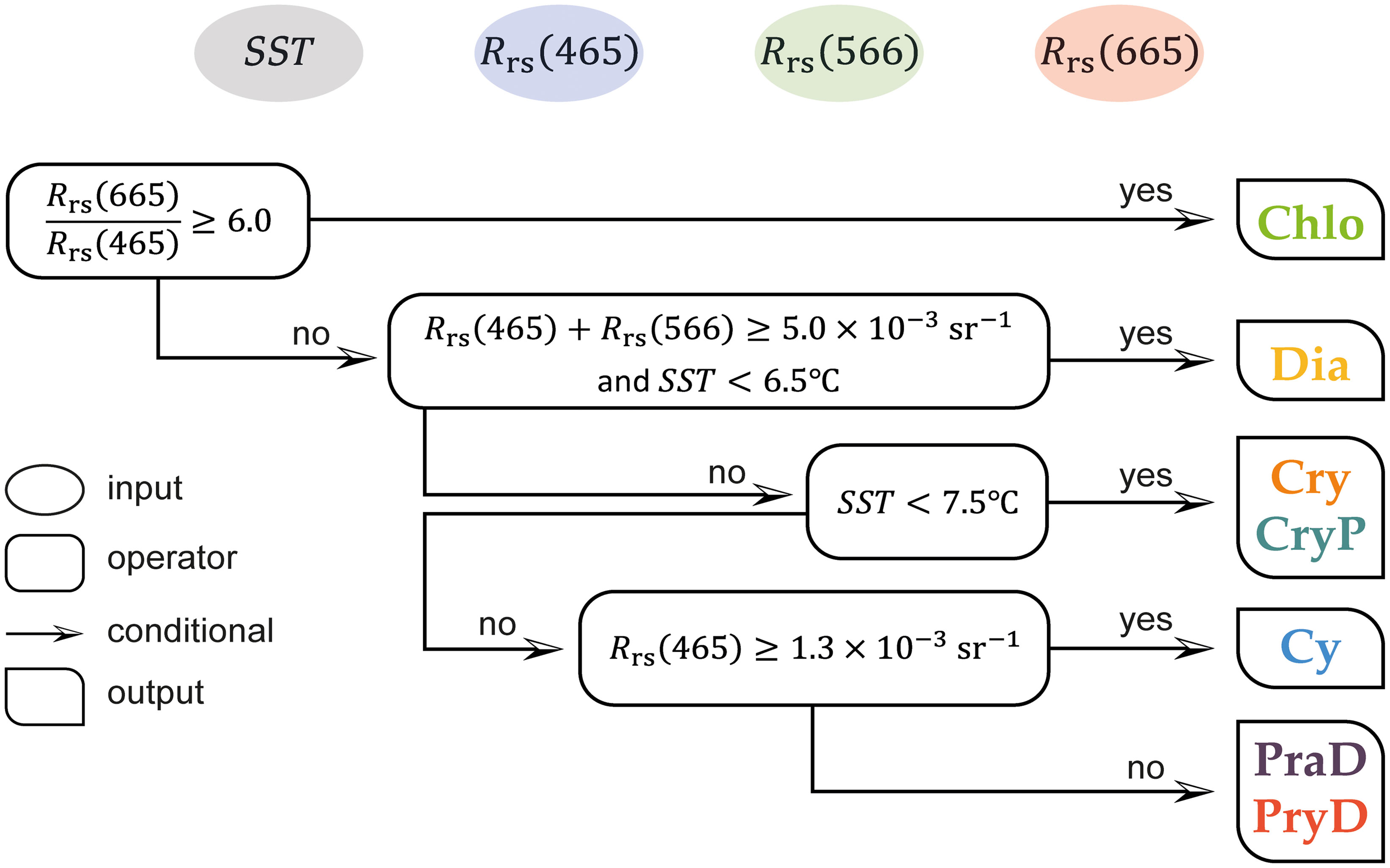
Figure 10 Idealized framework to separate the different phytoplankton assemblages using satellite-derived sea surface temperature (SST) and remote sensing reflectance in the blue (R_rs (465)), green (R_rs (566)), and red (R_rs (665)) regions of the spectrum.

Firstly, the group Chlo presented the highest values of a_cdom (465) and b_bp (665), resulting in low values of R_rs (465) and very high values of R_rs (665) and, consequently, were found in reddish waters. Considering this, using a simple threshold of the ratio R_rs (665)/R_rs (465), the group Chlo can be separated from others. Secondly, the lowest values of a_cdom and a_nap for group Dia resulted in the highest values of R_rs (465) and R_rs (566), comparatively to other groups. Thus, the sum of R_rs in these two wavelengths is used to target group Dia, and SST is also included to better distinguish it from group Cy.

In a third step, taking advantage of different temperature niches occupied by the phytoplankton assemblages, another threshold is used to separate groups Cry and CryP from groups Cy, PraD, and PryD. Finally, the lower a_cdom of Cy, and its influence on R_rs (465), is used to separate this group from PraD and PryD (Figure 10).

In a simple validation exercise, the presented framework was applied to the in situ R_rs and SST measurements to verify its coherence. When compared to the original discrimination of the seven phytoplankton assemblages (re-grouped in five, as in Figure 10; n = 72) determined by the PCA/HCA method, the result of this empirical inversion succeeded for 92% of the samples. The samples where this procedure failed refer mainly to some isolated groups in the context of other dominant groups in the same field campaign, as for example a single PraD (Figure 5D) and a Dia sample (Figure 5H).

To test the applicability of this framework in real imagery, we processed two Landsat 8 images from 2017 (April 4 and May 15, stars in Figure 9B), downloaded as Level-1 Collection 2 data and distributed by the United States Geological Survey (USGS). The R_rs(λ) thresholds presented in Figure 10 were tested and adjusted while contemplating the Spectral Response Function of the Operational Land Imager (OLI) of bands 2 (blue), 3 (green), and 4 (red). The two images were atmospherically-corrected using the dark spectrum fitting algorithm implemented in ACOLITE software (Vanhellemont, 2019; Vanhellemont, 2020c). For SST retrieval, the images of the Thermal Infrared Sensor (TIRS) were processed using the Thermal Atmospheric Correction Tool (TACT), also implemented in ACOLITE (Vanhellemont, 2020a; Vanhellemont, 2020b).

The application of the proposed framework in the two images (Figure 11) successfully targeted the dominance of group Dia in early April, as both R_rs values in the blue and green were higher than 0.005 sr^-1 and SST values were the lowest when compared to other periods. Following the freshet, the classification of the image from mid-May also could detect the presence of the group Cry/CryP in nearshore waters of BSI, while the group Dia was more restricted to offshore waters. The occurrence of group Cy at this period of the year is probably a misclassification due to the overestimation of R_rs in the blue region from the atmospheric correction procedure (see Mabit et al., 2022). In this case, the classified group Cy would actually represent a dominance of phytoplankton assemblages from groups PraD and/or PryD. Overall, the application of the framework in remote sensing imagery showed to be suitable.

FIGURE 11

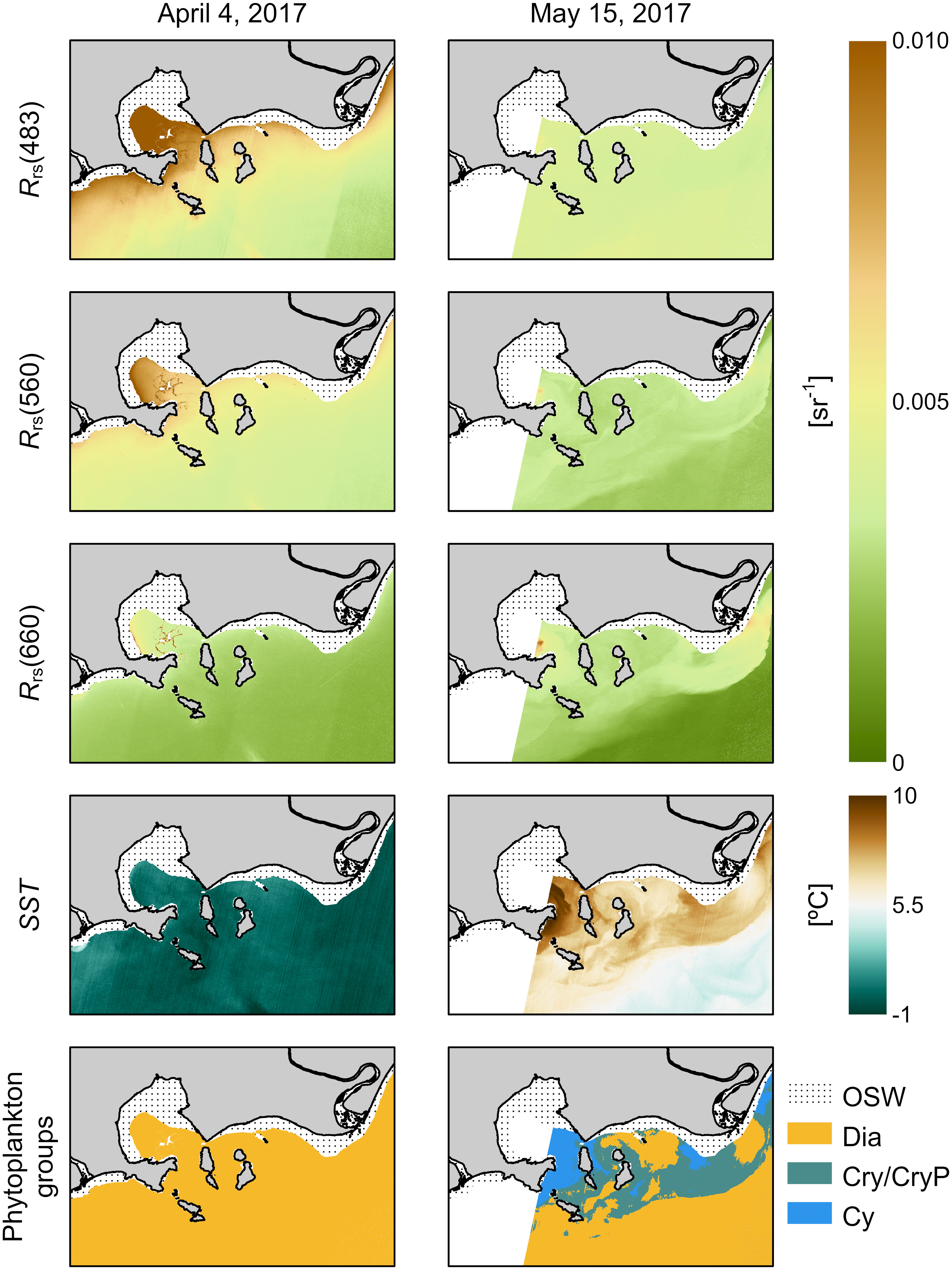
Figure 11 Application of the exposed framework shown in Figure 10 in satellite images of the Operational Land Imager (OLI) and the Thermal Infrared Sensor (TIRS) of Landsat 8. The atmospherically-corrected images of the blue, green, and red bands, the sea surface temperature, and the resulting classification of the groups of phytoplankton assemblages are shown for two dates: April 4 and May 15, 2017. OSW, optically-shallow waters.

4 Discussion

The potential for identification of major phytoplankton assemblages from pigment concentrations and <20 µm autotrophic cell abundances, in a dynamic nearshore subarctic environment, was evaluated. The combined PCA and HCA techniques applied to these proxies demonstrated to be a good indicator of distinctive communities of phytoplankton in the studied area, and it was confirmed, to some extent, by the LM taxonomy analysis. This dataset was comprehensive in terms of temporal (seasonal, from mid-spring to early fall) and spatial (order of 10⁰ to 10¹ km) scales. However, winter conditions, early phytoplankton spring bloom and pre-bloom (March-April), and mid-summer (August) conditions were missing.

The seven clusters revealed relevant characteristics associated to the following groups (Figure 3; Table S1): prasinophytes and dinoflagellates (PraD); prymnesiophytes and dinoflagellates (PryD); cyanobacteria (Cy); diatoms (Dia); cryptophytes (Cry); cryptophytes and prasinophytes (CryP); and chlorophytes (Chlo). These phytoplankton assemblages have been reported elsewhere in subarctic and temperate estuaries and coastal areas (Roy et al., 1996; Vallières et al., 2008; Vaulot et al., 2008; Blais et al., 2022). However, the nomenclature adopted in this study reflects pigment ratios characteristics used to distinguish the major phytoplankton assemblages but are not necessarily related to higher biomass or numerical dominance of one or another taxonomic class.

Flow cytometry and HPLC pigment analysis revealed complementary to each other on assigning the major classes of phytoplankton assemblages. For example, the presence of certain pigments (e.g., prasinoxanthin, 19’-hexanoyloxyfucoxanthin) allowed the determination of groups PraD and PryD, and they also presented a high number of picoeukaryotes (Figure 3). Micromonas pusilla and Chrysocromulina sp. are candidate species to be representative of these clusters, respectively, as they are ubiquitous in cold marine environments (see review of Vaulot et al., 2008). In addition, the ability to count the phycoerythrin-containing cyanobacteria using flow cytometry, while phycoerythrin is a pigment not detected by standard HPLC method, was an asset to identify assemblages dominated by cyanobacteria (group Cy), which is probably related to Synechococcus sp.

The biomass distribution along the size spectrum of phytoplankton communities brings with them relevant ecological information (Cloern, 2018; and references therein). The approach of Uitz et al. (2006) partitioned the relative contribution to Chla of three different size classes, and it showed coherency with our interpretation of community structure of the seven identified groups. The fractional contribution of picophytoplankton to Chla (f_pico) estimated from HPLC pigments ($f_{\text{pico}}^{\text{HPLC}}$) and from flow cytometry ($f_{\text{pico}}^{\text{FC}}$) were coherent, especially for groups PraD and Cy (Figure 4A).

The overall dominance of $f_{\text{micro}}^{\text{HPLC}}$ over other fractions was noticeable for most of the phytoplankton assemblages, and comparable to other boreal coastal regions, such as in the Western English Channel and North Sea (Barnes et al., 2014). The general higher contribution of f_micro is expected in areas with relatively high biomass (Chla) and replenished nutrient conditions (Cloern, 2018; Brewin et al., 2019). The dispersion from f_micro (right corner of the ternary diagram shown in Figure 4B) towards f_nano (upper corner), for Cry, Cryp, and PryD, and towards f_pico (left corner), for PraD and Cy, agreed with the inferred characteristics of each group.

The samples from the middle of the Lower St. Lawrence Estuary (at PMZA station), collected from mid-summer to fall season (Table 1), presented only two phytoplankton assemblages (Dia and PraD), but relatively higher biomass compared to BSI. The nearshore BSI region has more variability in terms of physical and optical conditions than the PMZA location and, consequently, a more diverse microbial community, including phytoplankton, is expected. Although Dia and PraD assemblages were found in both PMZA and BSI, their nutrient and physical environments were very distinctive (Figure 6 and Table 2). The higher concentrations of all nutrients and salinity at PMZA are due to upwelled waters in the Lower St. Lawrence Estuary (Therriault et al., 1990) while BSI is influenced by the Gulf of St. Lawrence waters (see Koutitonsky and Bugden, 1991).

The seasonal variability of the phytoplankton assemblages is a common feature in temperate and polar coastal waters and estuaries (e.g., Ansotegui et al., 2003; Trefault et al., 2021). In addition, local river discharge in these environments is a major driver of phytoplankton composition (Domingues et al., 2005), biomass and production, particularly during the spring freshet (Malone et al., 1988). Overall, we found that the seasonal succession of phytoplankton assemblages in surface waters of BSI is intrinsically related to changes in the environmental niches that are largely driven by bio-optical conditions and sea surface temperature (SST).

Before the spring freshet, the group Dia fully occupied BSI surface waters, as expected for high-latitude spring blooms dominated by large cells (diatoms) (Tremblay et al., 2006; Carstensen et al., 2015). The low nutrient concentrations found during BSI-1 campaign suggest that phytoplankton growth was nutrient-limited at the time. While silicate depletion has been found to be responsible for the termination of an Arctic diatom bloom (Krause et al., 2019), the fact that silicate concentrations of ~0.2 – 1.1 µM persisted after nitrate had reached extremely low values of <0.1 µM indicates that the latter presumably drives bloom termination in the surface waters of BSI (Figure 6). A major shift in the coastal light environment occurs when freshet brings massive concentration of terrigenous optical constituents.

During higher riverine discharges, the assemblages associated with cryptophytes (Cry and CryP) occupy the waters of BSI. The assemblages associated with chlorophytes (Chlo) were also found during the spring freshet and, due to the proximity of the riverine discharges, the highest light absorption and the most turbid conditions conferred to them less biomass compared to other assemblages.

After freshet and with warmer SST, the assemblages composed by dinoflagellates co-occurring with smaller phytoplankton cells (PraD and PryD) replace groups Cry and CryP in BSI. These assemblages were characterized by nitrate-depleted conditions just after their first appearance in BSI-3 (Figure 9), and by lower concentration of phosphate. Nitrate-depleted conditions were also found to be associated with phytoplankton communities related to small prymnesiophytes and prasinophytes in the North Atlantic and Chukchi Sea (Sieracki et al., 1993; Hill et al., 2005). Notably, the occurrence, or even blooms, of the toxic dinoflagellate A. tamarense are likely associated to these two groups, as previously reported in summer for BSI (Weise et al., 2002) and the Lower St. Lawrence Estuary (Fauchot et al., 2008; Roy et al., 2021).

At the end of summer and throughout fall, the assemblage associated with a high abundance of PE-containing cyanobacteria (Cy) dominates BSI waters. However, the environmental niche they occupy is distinguishable from those of PraD and PryD only by fall (BSI-7), when nitrate concentration levels are replenished, and saltier (and less absorbing) waters from the Gulf of St. Lawrence are found.

The seasonal variability of surface nutrients followed the general pattern of the Gulf of St. Lawrence, especially regarding the establishment of nitrate-depleted conditions in summer (Tremblay et al., 2000; Blais et al., 2019). Nutrient concentrations in the nearshore and coastal areas of the Bay of Sept-Îles were consistently lower than those of upwelled waters in the Lower St. Lawrence Estuary (AZMP buoy, Blais et al., 2019).

The ratio $\left[{\text{NO}}_3^{-}\left] : \right[{\text{PO}}_4^{3-}\right]$ was consistently lower than the Redfield value (16:1) but showed large differences between phytoplankton assemblages (Table 2). The lowest values observed for this ratio here are typical of coastal areas, including estuaries, indicating that N is generally the limiting factor for phytoplankton growth (Howarth et al., 2021; and references therein). Moreover, Howarth et al. (2021) also demonstrated that, in addition to the contribution of continental runoff to nutrient loads in coastal areas, the adjacent ocean also strongly affects nutrient availability in these areas. This is consistent with the observed nitrate concentrations in BSI during late fall.

The seasonal (spring to fall) succession of phytoplankton assemblages in BSI region exhibit a shift from large cells, in the spring bloom (Group Dia), to smaller ones (nano- and pico-phytoplankton size classes) from summer to fall. This shift started after the spring freshet, towards nanophytoplankton (cryptophytes, groups Cry and CryP), followed by pico- and nano-eukaryotes such as those of groups PraD and PryD, coexisting with dinoflagellates, and finally cyanobacteria (group Cy).

The CDOM-laden waters of BSI makes the a_cdom a determining IOP in shaping the R_rs , especially at shorter wavelengths (~ <600 nm). Another characteristic of BSI waters (and other nearshore zones of the St. Lawrence Estuary; see Araújo and Bélanger, 2022) is the generally flatter spectral shape of the particulate backscattering coefficient (approximately −1 < γ < 0.5) comparatively to other coastal waters (e.g., Antoine et al., 2011). Furthermore, the mass-specific b_bp(λ) is very low compared to other regions, a characteristic of the particulate and dissolved organic-rich waters of BSI (Araújo and Bélanger, 2022). This is also reflected in the relatively lower R_rs(λ) particularly in the red region of the spectrum, expected for a determined concentration of particles, when compared to other regions (Mabit et al., 2022).

Phytoplankton absorption (a_phy ) represents a small fraction of the total absorption budget in BSI and, consequently, R_rs(λ) signals are more sensitive to other optically active constituents than phytoplankton itself. This result implies that algorithms used to discriminate major phytoplankton assemblages that rely only on phytoplankton optical properties may have limited applications in BSI, as it is the case for other optically complex waters (e.g., Arctic ocean; Reynolds and Stramski, 2019). Nevertheless, significant differences in a_phy spectra between some groups were found. Moreover, analysis of the spectral shape of a_phy and the Chla-specific a_phy also revealed significant differences in the seasonal domain (Araújo and Bélanger, 2022). Taking these results into consideration, the phytoplankton absorption can be an asset to assess the major phytoplankton assemblages in BSI, as demonstrated for diverse locations by other studies (e.g., Hoepffner and Sathyendranath, 1991; Hoepffner and Sathyendranath, 1993; Devred et al., 2006; Oliveira et al., 2021; Sun et al., 2022).

Recent satellite missions and respective sensors covers the blue (~465 nm), green (~566 nm), and red (~665 nm) region of the spectrum, and with a relevant spatial resolution (order of ~10¹ m) for the scale of this study (see review of Werdell et al., 2018), allowing the retrieval of the remote sensing reflectance (R_rs ) in these spectral bands. Another common satellite-derived parameter is the sea surface temperature (Minnett et al., 2019). Temperature is a major controlling factor of phytoplankton phenology (e.g., Trombetta et al., 2019) and it was found to explain well the phytoplankton primary production in the estuary and Gulf of St. Lawrence, under low nutrient concentration circumstances (Babin et al., 1991). The results of the framework shown in Figure 10 and its application in remote sensing imagery (Figure 11) demonstrated that current Earth Observation satellites can be used to infer the general seasonal pattern of the major phytoplankton assemblages in the BSI region.

Although the proposed approach is empirical in nature, its foundations remits to the general bio-optical background and physical environment in which each assemblage is contextualized. Operational satellite missions such as the Landsat 8-9, carrying the Operational Land Imager (OLI) and the Thermal Infrared Sensor (TIRS), Sentinel-2, carrying the MultiSpectral Instrument (MSI), and Sentinel-3, carrying the Ocean and Land Color Instrument (OLCI), are examples of sensors that could be used to investigate the phytoplankton assemblages in coastal zones. The suitability of this approach was shown in two scenes collected by Landsat 8 OLI/TIRS in spring 2017 (Figure 11). However, inherent constraints to optical remote sensing such as persistent cloud cover over target regions and difficulties in atmospheric correction (a necessary step to obtain R_rs from top-of-atmosphere radiances) in highly absorbing waters, as it is the case of nearshore regions of the estuary and Gulf of St. Lawrence (Mabit et al., 2022), will limit their application. Another important constrain to consider is the potential difference between temperatures used in this study, collected by in situ thermometers, and those collected by satellite radiometers, which are related to the sea surface skin temperature (see Donlon et al., 2002; Minnett et al., 2011).

Our general hypothesis that the composition of major assemblages in a coastal area will covary with temperature and the bulk optical environment (IOPs) is confirmed. Furthermore, the premise that the IOPs characterization is a necessary step to investigate the phytoplankton assemblages using optical approaches (as in Reynolds and Stramski, 2019) in a coastal area was also confirmed. The composition of phytoplankton assemblages likely reflected major traits that were shaped by different environmental niches.

5 Conclusions

Given the intrinsic dynamic of coastal and estuarine areas, phytoplankton ecology monitoring is a major challenge for scientists and, consequently, is often overlooked by stakeholders, managers, and policy makers. The application of the proposed framework to retrieve major phytoplankton assemblages using satellite imagery would favor the monitoring of essential biodiversity variables in coastal ecosystems (Muller-Karger et al., 2018), deriving information about their distribution and with potential to extend it to functional traits. Although developed in the context of the subarctic Bay of Sept-Îles, similar approaches could be successfully implemented in other coastal regions, especially those that experience strong seasonal variability.

In view of ecological modelling (coupled with hydrodynamical modelling, as for an aquatic system), the information about major phytoplankton assemblages derived by satellite could be integrated into a monitoring program including automated buoys to collect high frequency meteorological and oceanographic data (Eulerian perspective), and regular (space and time) field campaigns to collect target biogeochemical and optical parameters.

Global warming has an important role in restructuring major phytoplankton assemblages (Benedetti et al., 2021) and developing new tools to systematically monitor these microorganisms that are key to coastal ecosystems are urgent. Moreover, bringing the scientific knowledge developed in this study into a broader context, such as its mapping onto a Social-Ecological-Environmental System, as presented by Ferrario et al. (2022), would bring benefits to society.

Data availability statement

The datasets generated and analyzed for this study can be found in the St. Lawrence Global Observatory repository (https://ogsl.ca/en/home-slgo/), under the CHONe II project dataset.

Author contributions

CA and SB designed the study. CB was responsible for the flow cytometry analysis. J-ÉT was responsible for the nutrient analysis. SB contributed to fundraising, fieldwork, and software development for optical data processing. CA conducted fieldwork, laboratory analysis, curated the data, and wrote the first draft of the manuscript. All authors contributed to manuscript revision, read and approved the submitted version.

Funding

The data used in this study was mainly supported by the interdisciplinary project “Canadian Healthy Oceans Network” (CHONe-2), funded by the Natural Sciences and Engineering Research Council of Canada (NSERC) and its partners: Department of Fisheries and Ocean Canada and INREST (representing the Port of Sept-Îles and the city of Sept-Îles). CA was supported by PhD scholarships from CHONe-2 and the Fond de Recherche du Québec – Nature et technologies (FRQNT), through a grant of the Merit Scholarship Program for Foreign Students (PBEEE, grant number 263427). This study was also supported by a NSERC Discovery Grant of SB (RGPIN-2019-0670).

Acknowledgments

We acknowledge all people involved in the field work campaigns and laboratory analysis, with special thanks to Alexandre Théberge, Zélie Schuhmacher, and Dr. François-Pierre Danhiez. Thanks to Mélanie Simard and Julie Major for pigment analysis, to Sylvie Lessard for the phytoplankton identification and enumeration by light microscopy, to Gabrièle Deslongchamps and Jonathan Gagnon for nutrient analysis, to Raphäel Mabit for the C-OPS data processing, and to ARCTUS Inc. for kindly providing SST images processed using the TACT algorithm implemented in ACOLITE. CA also acknowledge Drs. Rick Reynolds and Michel Gosselin for insightful discussions in early versions of this manuscript.

Conflict of interest

The authors declare that the research was conducted in the absence of any commercial or financial relationships that could be construed as a potential conflict of interest.

Publisher’s note

All claims expressed in this article are solely those of the authors and do not necessarily represent those of their affiliated organizations, or those of the publisher, the editors and the reviewers. Any product that may be evaluated in this article, or claim that may be made by its manufacturer, is not guaranteed or endorsed by the publisher.

Supplementary material

The Supplementary Material for this article can be found online at: https://www.frontiersin.org/articles/10.3389/fmars.2022.1001098/full#supplementary-material

References

Ansotegui A., Sarobe A., Trigueros J. M., Urrutxurtu I., Orive E. (2003). Size distribution of algal pigments and phytoplankton assemblages in a coastal–estuarine environment: Contribution of small eukaryotic algae. J. Plankton Res. 25, 341–355. doi: 10.1093/plankt/25.4.341

CrossRef Full Text | Google Scholar

Antoine D., Siegel D. A., Kostadinov T., Maritorena S., Nelson N. B., Gentili B., et al. (2011). Variability in optical particle backscattering in contrasting bio-optical oceanic regimes. Limnol. Oceanogr. 56, 955–973. doi: 10.4319/lo.2011.56.3.0955

CrossRef Full Text | Google Scholar

Araújo C. A. S., Bélanger S. (2022). Variability of bio-optical properties in nearshore waters of the estuary and Gulf of St. Lawrence: Absorption and backscattering coefficients. Estuar. Coast. Shelf Sci. 264, 107688. doi: 10.1016/j.ecss.2021.107688

CrossRef Full Text | Google Scholar

Babin M., Therriault J.-C., Legendre L. (1991). Potential utilization of temperature in estimating primary production from remote sensing data in coastal and estuarine waters. Estuar. Coast. Shelf Sci. 33, 559–579. doi: 10.1016/0272-7714(91)90041-9

CrossRef Full Text | Google Scholar

Barnes M., Tilstone G., Smyth T., Suggett D., Astoreca R., Lancelot C., et al. (2014). Absorption-based algorithm of primary production for total and size-fractionated phytoplankton in coastal waters. Mar. Ecol. Prog. Ser. 504, 73–89. doi: 10.3354/meps10751

CrossRef Full Text | Google Scholar

Bélanger S., Carrascal-Leal C., Jaegler T., Larouche P., Galbraith P. (2017). Assessment of radiometric data from a buoy in the St. Lawrence estuary. J. Atmos. Ocean. Technol. 34, 877–896. doi: 10.1175/JTECH-D-16-0176.1

CrossRef Full Text | Google Scholar

Benedetti F., Vogt M., Elizondo U. H., Righetti D., Zimmermann N. E., Gruber N. (2021). Major restructuring of marine plankton assemblages under global warming. Nat. Commun. 12, 5226. doi: 10.1038/s41467-021-25385-x

PubMed Abstract | CrossRef Full Text | Google Scholar

Bidigare R. R., Van Heukelem L., Trees C. C. (2005). “Analysis of algal pigments by high-performance liquid chromatography,” in Algal culturing techniques. Ed. Andersen R. A. (Burlington, MA: Elsevier Academic Press), 327–345. doi: 10.1016/b978-012088426-1/50021-4

CrossRef Full Text | Google Scholar

Blais M., Galbraith P. S., Plourde S., Scarratt M., Devine L., Lehoux C. (2019). Chemical and biological oceanographic conditions in the estuary and gulf of st. Lawrence during 2018. DFO Can. Sci. Advis. Sec. Res. Doc. 059, 64p.

Google Scholar

Blais M.-A., Matveev A., Lovejoy C., Vincent W. F. (2022). Size-fractionated microbiome structure in subarctic rivers and a coastal plume across DOC and salinity gradients. Front. Microbiol. 12. doi: 10.3389/fmicb.2021.760282

CrossRef Full Text | Google Scholar

Bluteau C. E., Galbraith P. S., Bourgault D., Villeneuve V., Tremblay J.-É. (2021). Winter observations alter the seasonal perspectives of the nutrient transport pathways into the lower St. Lawrence estuary. Ocean Sci. 17, 1509–1525. doi: 10.5194/os-17-1509-2021

CrossRef Full Text | Google Scholar

Brewin R. J. W., Morán X. A. G., Raitsos D. E., Gittings J. A., Calleja M. L., Viegas M., et al. (2019). Factors regulating the relationship between total and size-fractionated chlorophyll-a in coastal waters of the red Sea. Front. Microbiol. 10. doi: 10.3389/fmicb.2019.01964

CrossRef Full Text | Google Scholar

Carstensen J., Klais R., Cloern J. E. (2015). Phytoplankton blooms in estuarine and coastal waters: Seasonal patterns and key species. Estuar. Coast. Shelf Sci. 162, 98–109. doi: 10.1016/j.ecss.2015.05.005

CrossRef Full Text | Google Scholar

Cloern J. E. (2001). Our evolving conceptual model of the coastal eutrophication problem. Mar. Ecol. Prog. Ser. 210, 223–253. doi: 10.3354/meps210223

CrossRef Full Text | Google Scholar

Cloern J. E. (2018). Why large cells dominate estuarine phytoplankton. Limnol. Oceanogr. 63, S392–S409. doi: 10.1002/lno.10749

CrossRef Full Text | Google Scholar

Cloern J. E., Foster S. Q., Kleckner A. E. (2014). Phytoplankton primary production in the world’s estuarine-coastal ecosystems. Biogeosciences 11, 2477–2501. doi: 10.5194/bg-11-2477-2014

CrossRef Full Text | Google Scholar

Cloern J. E., Jassby A. D. (2008). Complex seasonal patterns of primary producers at the land-sea interface. Ecol. Lett. 11, 1294–1303. doi: 10.1111/j.1461-0248.2008.01244.x

PubMed Abstract | CrossRef Full Text | Google Scholar

Devred E., Sathyendranath S., Stuart V., Maass H., Ulloa O., Platt T. (2006). A two-component model of phytoplankton absorption in the open ocean: Theory and applications. J. Geophys. Res. 111, C03011. doi: 10.1029/2005JC002880

CrossRef Full Text | Google Scholar

Domingues R. B., Barbosa A., Galvão H. (2005). Nutrients, light and phytoplankton succession in a temperate estuary (the guadiana, south-western Iberia). Estuar. Coast. Shelf Sci. 64, 249–260. doi: 10.1016/j.ecss.2005.02.017

CrossRef Full Text | Google Scholar

Donlon C. J., Minnett P. J., Gentemann C., Nightingale T. J., Barton I. J., Ward B., et al. (2002). Toward improved validation of satellite sea surface skin temperature measurements for climate research. J. Clim. 15, 353–369. doi: 10.1175/1520-0442(2002)015<0353:TIVOSS>2.0.CO;2

CrossRef Full Text | Google Scholar

Dreujou E., Desroy N., Carrière J., Tréau de Coeli L., McKindsey C. W., Archambault P. (2021). Determining the ecological status of benthic coastal communities: A case in an anthropized sub-arctic area. Front. Mar. Sci. 8. doi: 10.3389/fmars.2021.637546

CrossRef Full Text | Google Scholar

Edwards K. F., Thomas M. K., Klausmeier C. A., Litchman E. (2016). Phytoplankton growth and the interaction of light and temperature: A synthesis at the species and community level. Limnol. Oceanogr. 61, 1232–1244. doi: 10.1002/lno.10282

CrossRef Full Text | Google Scholar

Fauchot J., Saucier F. J., Levasseur M., Roy S., Zakardjian B. (2008). Wind-driven river plume dynamics and toxic alexandrium tamarense blooms in the st. Lawrence estuary (Canada): A modeling study. Harmful Algae 7, 214–227. doi: 10.1016/j.hal.2007.08.002

CrossRef Full Text | Google Scholar

Ferrario F., Araújo C. A. S., Bélanger S., Bourgault D., Carrière J., Carrier-Belleau C., et al. (2022). Holistic environmental monitoring in ports as an opportunity to advance sustainable development, marine science, and social inclusiveness. Elem. Sci. Anthr. 10, 1–21. doi: 10.1525/elementa.2021.00061

CrossRef Full Text | Google Scholar

Gibb S., Barlow R., Cummings D., Rees N., Trees C., Holligan P., et al. (2000). Surface phytoplankton pigment distributions in the Atlantic ocean: An assessment of basin scale variability between 50°N and 50°S. Prog. Oceanogr. 45, 339–368. doi: 10.1016/S0079-6611(00)00007-0

CrossRef Full Text | Google Scholar

Glibert P., Anderson D., Gentien P., Granéli E., Sellner K. (2005). The global, complex phenomena of harmful algal blooms. Oceanography 18, 136–147. doi: 10.5670/oceanog.2005.49

CrossRef Full Text | Google Scholar

Harley C. D. G., Randall Hughes A., Hultgren K. M., Miner B. G., Sorte C. J. B., Thornber C. S., et al. (2006). The impacts of climate change in coastal marine systems. Ecol. Lett. 9, 228–241. doi: 10.1111/j.1461-0248.2005.00871.x

PubMed Abstract | CrossRef Full Text | Google Scholar

Hill V., Cota G., Stockwell D. (2005). Spring and summer phytoplankton communities in the chukchi and Eastern Beaufort seas. Deep. Res. Part II Top. Stud. Oceanogr. 52, 3369–3385. doi: 10.1016/j.dsr2.2005.10.010

CrossRef Full Text | Google Scholar

Hintz N. H., Zeising M., Striebel M. (2021). Changes in spectral quality of underwater light alter phytoplankton community composition. Limnol. Oceanogr. 66, 3327–3337. doi: 10.1002/lno.11882

CrossRef Full Text | Google Scholar

Hoepffner N., Sathyendranath S. (1991). Effect of pigment composition on absorption properties of phytoplankton. Mar. Ecol. Prog. Ser. 73, 11–23. doi: 10.3354/meps073011

CrossRef Full Text | Google Scholar

Hoepffner N., Sathyendranath S. (1993). Determination of the major groups of phytoplankton pigments from the absorption spectra of total particulate matter. J. Geophys. Res. 98, 22789. doi: 10.1029/93JC01273

CrossRef Full Text | Google Scholar

Howarth R. W., Chan F., Swaney D. P., Marino R. M., Hayn M. (2021). Role of external inputs of nutrients to aquatic ecosystems in determining prevalence of nitrogen vs. phosphorus limitation of net primary productivity. Biogeochemistry 154, 293–306. doi: 10.1007/s10533-021-00765-z

CrossRef Full Text | Google Scholar

IOCCG (2014). Phytoplankton functional types from space. Ed. Sathyendranath S. (Dartmouth, Canada: IOCCG).

Google Scholar

IOCCG (2018). Ocean optics and biogeochemistry protocols for satellite ocean colour sensor validation. volume 1: Inherent optical property measurements and protocols: absorption coefficient. Eds. Neeley A. R., Mannino A. (Dartmouth, Canada: IOCCG). doi: 10.25607/OBP-119

CrossRef Full Text | Google Scholar

Koutitonsky V. G., Bugden G. L. (1991). The physical oceanography of the gulf of st. Lawrence: A review wilh emphasis on the synoptic variability of the motion. Can. Spec. Publ. Fish. Aquat. Sci. 113, 57–90.

Google Scholar

Kramer S. J., Siegel D. A. (2019). How can phytoplankton pigments be best used to characterize surface ocean phytoplankton groups for ocean color remote sensing algorithms? J. Geophys. Res. Ocean. 124, 7557–7574. doi: 10.1029/2019JC015604

CrossRef Full Text | Google Scholar

Krause J. W., Schulz I. K., Rowe K. A., Dobbins W., Winding M. H. S., Sejr M. K., et al. (2019). Silicic acid limitation drives bloom termination and potential carbon sequestration in an Arctic bloom. Sci. Rep. 9, 1–11. doi: 10.1038/s41598-019-44587-4

PubMed Abstract | CrossRef Full Text | Google Scholar

Le Quéré C., Harrison S. P., Colin Prentice I., Buitenhuis E. T., Aumont O., Bopp L., et al. (2005). Ecosystem dynamics based on plankton functional types for global ocean biogeochemistry models. Glob. Change Biol. 11, 2016–2040. doi: 10.1111/j.1365-2486.2005.1004.x

CrossRef Full Text | Google Scholar

Lindeman R. L. (1942). The trophic-dynamic aspect of ecology. Ecology 23, 399–417. doi: 10.2307/1930126

CrossRef Full Text | Google Scholar

Litchman E., de Tezanos Pinto P., Klausmeier C. A., Thomas M. K., Yoshiyama K. (2010). Linking traits to species diversity and community structure in phytoplankton. Hydrobiologia 653, 15–28. doi: 10.1007/s10750-010-0341-5

CrossRef Full Text | Google Scholar

Litchman E., Klausmeier C. A., Schofield O. M., Falkowski P. G. (2007). The role of functional traits and trade-offs in structuring phytoplankton communities: Scaling from cellular to ecosystem level. Ecol. Lett. 10, 1170–1181. doi: 10.1111/j.1461-0248.2007.01117.x

PubMed Abstract | CrossRef Full Text | Google Scholar

Lund J. W. G., Kipling C., Le Cren E. D. (1958). The inverted microscope method of estimating algal numbers and the statistical basis of estimations by counting. Hydrobiologia 11, 143–170. doi: 10.1007/BF00007865

CrossRef Full Text | Google Scholar

Mabit R., Araújo C. A. S., Singh R. K., Bélanger S. (2022). Empirical remote sensing algorithms to retrieve SPM and CDOM in québec coastal waters. Front. Remote Sens. 3. doi: 10.3389/frsen.2022.834908

CrossRef Full Text | Google Scholar

Malone T. C., Crocker L. H., Pike S. E., Wendler B. W. (1988). Influences of river flow on the dynamics of phytoplankton production in a partially stratified estuary. Mar. Ecol. Prog. Ser. 48, 235–249. doi: 10.3354/meps048235

CrossRef Full Text | Google Scholar

McMahon K. W., Ambrose W. G., Reynolds M. J., Johnson B. J., Whiting A., Clough L. M. (2021). Arctic Lagoon and nearshore food webs: Relative contributions of terrestrial organic matter, phytoplankton, and phytobenthos vary with consumer foraging dynamics. Estuar. Coast. Shelf Sci. 257, 107388. doi: 10.1016/j.ecss.2021.107388

CrossRef Full Text | Google Scholar

Minnett P. J., Alvera-Azcárate A., Chin T. M., Corlett G. K., Gentemann C. L., Karagali I., et al. (2019). Half a century of satellite remote sensing of sea-surface temperature. Remote Sens. Environ. 233, 111366. doi: 10.1016/j.rse.2019.111366

CrossRef Full Text | Google Scholar

Minnett P. J., Smith M., Ward B. (2011). Measurements of the oceanic thermal skin effect. Deep Sea Res. Part II Top. Stud. Oceanogr. 58, 861–868. doi: 10.1016/j.dsr2.2010.10.024

CrossRef Full Text | Google Scholar

Montagnes D. J. S., Berges J. A., Harrison P. J., Taylor F. J. R. (1994). Estimating carbon, nitrogen, protein, and chlorophyll a from volume in marine phytoplankton. Limnol. Oceanogr. 39, 1044–1060. doi: 10.4319/lo.1994.39.5.1044

CrossRef Full Text | Google Scholar

Morel A. (1974). “Optical properties of pure water and pure seawater,” in Optical aspects of oceanography. Eds. Jerlov N. G., Steeman-Nielsen E. (New York, NY, USA: Academic Press), 1–24.

Google Scholar

Morel A., Ahn Y.-H., Partensky F., Vaulot D., Claustre H. (1993). Prochlorococcus and Synechococcus: A comparative study of their optical properties in relation to their size and pigmentation. J. Mar. Res. 51, 617–649. doi: 10.1357/0022240933223963

CrossRef Full Text | Google Scholar

Morel A., Prieur L. (1977). Analysis of variations in ocean color. Limnol. Oceanogr. 22, 709–722. doi: 10.4319/lo.1977.22.4.0709

CrossRef Full Text | Google Scholar

Muller-Karger F. E., Hestir E., Ade C., Turpie K., Roberts D. A., Siegel D., et al. (2018). Satellite sensor requirements for monitoring essential biodiversity variables of coastal ecosystems. Ecol. Appl. 28, 749–760. doi: 10.1002/eap.1682

PubMed Abstract | CrossRef Full Text | Google Scholar

Neukermans G., Reynolds R. A., Stramski D. (2016). Optical classification and characterization of marine particle assemblages within the western Arctic ocean. Limnol. Oceanogr. 61, 1472–1494. doi: 10.1002/lno.10316

CrossRef Full Text | Google Scholar

Normandeau A., Lajeunesse P., St-Onge G. (2013). Shallow-water longshore drift-fed submarine fan deposition (Moisie river delta, Eastern Canada). Geo-Marine Lett. 33, 391–403. doi: 10.1007/s00367-013-0336-0

CrossRef Full Text | Google Scholar

Oliveira A. L., Rudorff N., Kampel M., Sathyendranath S., Pompeu M., Detoni A. M. S., et al. (2021). Phytoplankton assemblages and optical properties in a coastal region of the south Brazil bight. Cont. Shelf Res. 227, 104509. doi: 10.1016/j.csr.2021.104509

CrossRef Full Text | Google Scholar

Reynolds R. A., Stramski D. (2019). Optical characterization of marine phytoplankton assemblages within surface waters of the western Arctic ocean. Limnol. Oceanogr. 64, 2478–2496. doi: 10.1002/lno.11199

PubMed Abstract | CrossRef Full Text | Google Scholar

Roselli L., Litchman E. (2017). Phytoplankton traits, functional groups and community organization. J. Plankton Res. 39, 491–493. doi: 10.1093/plankt/fbx019

CrossRef Full Text | Google Scholar

Roy S., Chanut J., Gosselin M., Sime-Ngando T. (1996). Characterization of phytoplankton communities in the lower St. Lawrence estuary using HPLC-detected pigments and cell microscopy. Mar. Ecol. Prog. Ser. 142, 55–73. doi: 10.3354/meps142055

CrossRef Full Text | Google Scholar

Roy S., Pitcher G. C., Kudela R. M., Smith M. E., Bernard S., Mazeran C. (2021). “Ocean colour remote sensing of dinoflagellate blooms associated with paralytic shellfish poisoning,” in Observation of harmful algal blooms with ocean colour radiometry. Eds. Bernard S., Kudela R. M., Lain L.R., Pitcher G. C. (Dartmouth, Canada: International Ocean Colour Coordinating Group), 39–50. doi: 10.25607/OBP-1042

CrossRef Full Text | Google Scholar

Salvador S., Chan P. (2004). “Determining the number of clusters/segments in hierarchical clustering/segmentation algorithms,” in 16th IEEE international conference on tools with artificial intelligence, (Boca Raton, FL, USA: IEEE comput. soc). 576–584. doi: 10.1109/ICTAI.2004.50

CrossRef Full Text | Google Scholar

Sathyendranath S., Prieur L., Morel A. (1989). A three-component model of ocean colour and its application to remote sensing of phytoplankton pigments in coastal waters. Int. J. Remote Sens. 10, 1373–1394. doi: 10.1080/01431168908903974

CrossRef Full Text | Google Scholar

Shaw J.-L. (2019). Hydrodynamique de la Baie de Sept-Îles, M.Sc. Thesis. (Rimouski, QC, Canada: Université du Québec à Rimouski).

Google Scholar

Sieracki M. E., Verity P. G., Stoecker D. K. (1993). Plankton community response to sequential silicate and nitrate depletion during the 1989 north Atlantic spring bloom. Deep. Res. Part II 40, 213–225. doi: 10.1016/0967-0645(93)90014-E

CrossRef Full Text | Google Scholar

Sokal R. R., Rohlf F. J. (1962). The comparison of dendrograms by objective methods. Taxon 11, 33–40. doi: 10.2307/1217208

CrossRef Full Text | Google Scholar

Stomp M., Huisman J., Stal L. J., Matthijs H. C. P. (2007). Colorful niches of phototrophic microorganisms shaped by vibrations of the water molecule. ISME J. 1, 271–282. doi: 10.1038/ismej.2007.59

PubMed Abstract | CrossRef Full Text | Google Scholar

Sun X., Shen F., Brewin R. J. W., Li M., Zhu Q. (2022). Light absorption spectra of naturally mixed phytoplankton assemblages for retrieval of phytoplankton group composition in coastal oceans. Limnol. Oceanogr. 67, 946–961. doi: 10.1002/lno.12047

CrossRef Full Text | Google Scholar

Therriault J.-C., Legendre L., Demers S. (1990). “Oceanography and ecology of phytoplankton in the St.Lawrence estuary,” in Oceanography of a Large-scale estuarine system. Eds. El-Sabh M., Silverberg N., (New York, NY, USA: Springer-Verlag) 269–295. doi: 10.1007/978-1-4615-7534-4_12

CrossRef Full Text | Google Scholar

Trefault N., de la Iglesia R., Moreno-Pino M., Lopes dos Santos A., Gérikas Ribeiro C., Parada-Pozo G., et al. (2021). Annual phytoplankton dynamics in coastal waters from fildes bay, Western Antarctic peninsula. Sci. Rep. 11, 1368. doi: 10.1038/s41598-020-80568-8

PubMed Abstract | CrossRef Full Text | Google Scholar

Tremblay G., Belzile C., Gosselin M., Poulin M., Roy S., Tremblay J. (2009). Late summer phytoplankton distribution along a 3500 km transect in Canadian Arctic waters: Strong numerical dominance by picoeukaryotes. Aquat. Microb. Ecol. 54, 55–70. doi: 10.3354/ame01257

CrossRef Full Text | Google Scholar

Tremblay J.É., Legendre L., Klein B., Therriault J.-C. (2000). Size-differential uptake of nitrogen and carbon in a marginal sea (Gulf of st. Lawrence, canada): Significance of diel periodicity and urea uptake. Deep. Res. Part II Top. Stud. Oceanogr. 47, 489–518. doi: 10.1016/S0967-0645(99)00116-2

CrossRef Full Text | Google Scholar

Tremblay J.É., Michel C., Hobson K. A., Gosselin M., Price N. M. (2006). Bloom dynamics in early opening waters of the Arctic ocean. Limnol. Oceanogr. 51, 900–912. doi: 10.4319/lo.2006.51.2.0900

CrossRef Full Text | Google Scholar

Trombetta T., Vidussi F., Mas S., Parin D., Simier M., Mostajir B. (2019). Water temperature drives phytoplankton blooms in coastal waters. PloS One 14, 1–28. doi: 10.1371/journal.pone.0214933

CrossRef Full Text | Google Scholar

Uitz J., Claustre H., Morel A., Hooker S. B. (2006). Vertical distribution of phytoplankton communities in open ocean: An assessment based on surface chlorophyll. J. Geophys. Res. 111, C08005. doi: 10.1029/2005JC003207

CrossRef Full Text | Google Scholar

Vallières C., Retamal L., Ramlal P., Osburn C. L., Vincent W. F. (2008). Bacterial production and microbial food web structure in a large arctic river and the coastal Arctic ocean. J. Mar. Syst. 74, 756–773. doi: 10.1016/j.jmarsys.2007.12.002

CrossRef Full Text | Google Scholar

Vandevelde T., Legendre L., Therriault J.-C., Demers S., Bah A. (1987). Subsurface chlorophyll maximum and hydrodynamics of the water column. J. Mar. Res. 45, 377–396. doi: 10.1357/002224087788401151

CrossRef Full Text | Google Scholar

Vanhellemont Q. (2019). Adaptation of the dark spectrum fitting atmospheric correction for aquatic applications of the landsat and sentinel-2 archives. Remote Sens. Environ. 225, 175–192. doi: 10.1016/j.rse.2019.03.010

CrossRef Full Text | Google Scholar

Vanhellemont Q. (2020a). Automated water surface temperature retrieval from landsat 8/TIRS. Remote Sens. Environ. 237, 111518. doi: 10.1016/j.rse.2019.111518

CrossRef Full Text | Google Scholar

Vanhellemont Q. (2020b). Combined land surface emissivity and temperature estimation from landsat 8 OLI and TIRS. ISPRS J. Photogramm. Remote Sens. 166, 390–402. doi: 10.1016/j.isprsjprs.2020.06.007

CrossRef Full Text | Google Scholar

Vanhellemont Q. (2020c). Sensitivity analysis of the dark spectrum fitting atmospheric correction for metre- and decametre-scale satellite imagery using autonomous hyperspectral radiometry. Opt. Express 28, 29948. doi: 10.1364/OE.397456

PubMed Abstract | CrossRef Full Text | Google Scholar

Vaulot D., Eikrem W., Viprey M., Moreau H. (2008). The diversity of small eukaryotic phytoplankton (≤3 μm) in marine ecosystems. FEMS Microbiol. Rev. 32, 795–820. doi: 10.1111/j.1574-6976.2008.00121.x

PubMed Abstract | CrossRef Full Text | Google Scholar

Ward J. H. (1963). Hierarchical grouping to optimize an objective function. J. Am. Stat. Assoc. 58, 236–244. doi: 10.1080/01621459.1963.10500845

CrossRef Full Text | Google Scholar

Wassmann P., Duarte C. M., Agustí S., Sejr M. K. (2011). Footprints of climate change in the Arctic marine ecosystem. Glob. Change Biol. 17, 1235–1249. doi: 10.1111/j.1365-2486.2010.02311.x

CrossRef Full Text | Google Scholar

Weise A. M., Levasseur M., Saucier F. J., Senneville S., Bonneau E., Roy S., et al. (2002). The link between precipitation, river runoff, and blooms of the toxic dinoflagellate Alexandrium tamarense in the St. Lawrence. Can. J. Fish. Aquat. Sci. 59, 464–473. doi: 10.1139/f02-024

CrossRef Full Text | Google Scholar

Werdell P. J., McKinna L. I. W., Boss E., Ackleson S. G., Craig S. E., Gregg W. W., et al. (2018). An overview of approaches and challenges for retrieving marine inherent optical properties from ocean color remote sensing. Prog. Oceanogr. 160, 186–212. doi: 10.1016/j.pocean.2018.01.001

PubMed Abstract | CrossRef Full Text | Google Scholar

Winder M., Carstensen J., Galloway A. W. E., Jakobsen H. H., Cloern J. E. (2017). The land-sea interface: A source of high-quality phytoplankton to support secondary production. Limnol. Oceanogr. 62, S258–S271. doi: 10.1002/lno.10650

CrossRef Full Text | Google Scholar

Zapata M., Rodríguez F., Garrido J. (2000). Separation of chlorophylls and carotenoids from marine phytoplankton: A new HPLC method using a reversed phase C8 column and pyridine-containing mobile phases. Mar. Ecol. Prog. Ser. 195, 29–45. doi: 10.3354/meps195029

CrossRef Full Text | Google Scholar

Zhang X., Hu L., He M.-X. (2009). Scattering by pure seawater at high salinity. Opt. Express 17, 5698–5710. doi: 10.1364/OE.17.012685

PubMed Abstract | CrossRef Full Text | Google Scholar